Frequency Hopping Joint Radar-Communications with Hybrid Sub-pulse Frequency and Duration Modulation
Abstract
Frequency-hopping (FH) joint radar-communications (JRC) can offer excellent security for integrated sensing and communication systems. However, existing JRC schemes mainly embed information using only the sub-pulse frequencies and hence the data rate is limited. In this paper, we propose to use both sub-pulse frequencies and durations for information modulation, leading to higher communication data rates. For information demodulation, we propose a novel scheme by using the time-frequency analysis (TFA) technique and a ‘you only look once’ (YOLO)-based detection system. As such, our system does not require channel estimation, simplifying the transmission signal frame design. Simulation results demonstrate the effectiveness of our scheme, and show that it is robust against the Doppler shift and timing offset between the transceiver and the communication receiver.
Index Terms:
Joint radar-communications, waveform design, YOLO.I Introduction
The frequency-hopping (FH) joint radar-communications systems (JRC) [1, 2, 3, 4, 5] have become more and more prevalent in both military and civil applications, e.g., airborne, shipborne, ground-based combat systems, the connected autonomous vehicle (CAV). The most popular FH JRC systems include multiple-input multiple-output orthogonal frequency division multiplexing (MIMO-OFDM), multi-Carrier AgilE phaSed Array Radar (CAESAR), and FH-MIMO[2].
A key challenge in FH JRC is to embed/modulate data (onto frequency sub-pulses) at the transceiver and demodulate the signal at the receiver. For data embedding, the most dominant technique is the index modulation (IM), which utilizes frequency selection/combination and/or antenna selection/permutation for data representation. Specifically, the data bits are embedded by selecting different sets of sub-pulse frequency (i.e., frequency combination) and allocating them to different antennas (i.e., antennas permutation). For data demodulation, the optimal demodulator can be based on the maximum likelihood principle [3], while sub-optimal methods, which require lower computation complexities, are based on compressive sensing (CS) or discrete Fourier transform (DFT) [2]. However, the performance of these methods depends on the accuracy of channel estimation. Unfortunately, a long training sequence necessary for accurate channel estimation is not always feasible. This is because a long training sequence reduces the communication fraction over the whole time frame, thus decreasing the data bit rate. In particular, the data embedding schemes using both sub-pulse frequency combinations and antenna permutations require complex demodulation techniques that are prone to demodulation error. On the other hand, the data embedding scheme using only the sub-pulse frequency combination has a limited data transmission rate.
This paper proposes novel techniques to embed and demodulate data in an FH JRC system to increase the data rate and reduce the demodulation error. For data embedding, we use both sub-pulse frequency and duration, therefore increasing the data transmission rate compared to only using the sub-pulse frequency. For data demodulation, we propose a novel scheme based on the signal’s time-frequency image (TFI) and a YOLO-based detection system. This demodulation scheme does not require channel estimation and is robust to the Doppler shift and the timing offset between the transceiver and the communication receiver. Moreover, the proposed data embedding and demodulation schemes are spatially flexible and not limited to the sidelobe of the transmit beampattern, since the data is not embedded by utilizing the phase or amplitude of the beampattern sidelobe.
II System and Signals
II-A System Overview
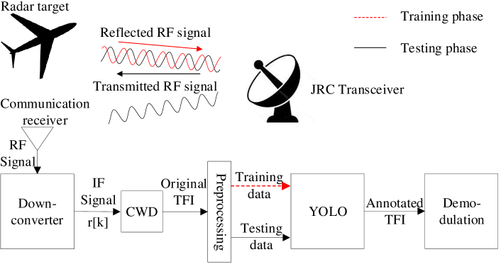
We consider a ground-to-air JRC system, where the JRC transceiver is located on the ground and the communication receiver is mounted on an aircraft or a high-altitude platform (HAP), as illustrated in Fig. 1. For sensing, the JRC transceiver transmits the radio frequency (RF) signal and processes the reflected RF signal to determine target’s position and velocity. For data transmission, the communication receiver obtains the RF signal from the JRC transceiver and demodulate the embedded data. In such a system, the line-of-sight (LoS) path dominates, and non-LoS paths are negligible. At the transceiver or communication receiver, the received RF signal is down-converted into the intermediate frequency (IF) signal and sampled at sampling frequency to generate a discrete-time signal as
| (1) |
Here, is the sample index which increases every , and are the transmitted and received signal samples, respectively, and is the complex additive white Gaussian noise (AWGN). The JRC system uses a pulse wave (PW) waveform with a duty cycle , where and are the pulse width and pulse repetition intervals, respectively. The received signal at the communication receiver is then used to generate the Choi-Williams distribution time-frequency image (CWD-TFI). Next, the CWD-TFI is preprocessed in the Preprocessing block to generate the training and testing data for the YOLO detection system. The training process of the YOLO detection system is demonstrated by the dashed line in Fig. 1 using the training data. The trained YOLO detection system and the testing CWD-TFIs are used to generate the annotated CWD-TFIs, which are used to demodulate the embedded data.
II-B Signals Model
The JRC system uses FH signals with each signal pulse being divided into sub-pulses (i.e., hops) with different frequencies and durations. Let denote the FH sequence and denote the sub-pulse duration sequence. The JRC signals in each pulse is represented by
| (2) | ||||
| signal amplitude, | ||||
III Data Embedding Schemes
In this work, we use the Costas arrays to generate the FH sequence of each signal pulse in one of the data embedding schemes. Using the Costas array, an FH signal possesses a narrow peak at the origin of its ambiguity function (AF) and low sidelobes elsewhere, which is desirable for the radar measurement (i.e., range and speed) accuracy. Details of the Costas arrays, their construction, and characteristics can be found in [6, Ch. 5].
We propose two data embedding techniques, namely Random and Costas-based schemes. Unlike existing studies that only utilize sub-pulse frequencies to convey information, both sub-pulse frequencies and durations are used in our proposed schemes. We first design the codebooks and of the Random and Costas-based schemes, respectively. Then, for each embedding scheme, data bits are embedded by mapping each element of the corresponding codebook to a symbol. Let be the selection set of the sub-pulse frequency, where is the fundamental frequency. Let be the selection set of the sub-pulse duration, where is the number of sub-pulse duration selections. The codebooks and are designed as follows.
-
•
Random scheme: is designed by selecting each sub-pulse frequency from the frequency set , and selecting each sub-pulse duration from the duration set as
(3) (4) Here, condition (4) means every two consecutive sub-pulse frequencies are not equal, which is necessary for the data demodulation technique that will be presented in Section V.
-
•
Costas-based scheme: Unlike the Random scheme, for designing , each sub-pulse frequency is not individually selected. Instead, the whole FH sequence of each signal pulse is selected from the Costas-based FH sequence defined as follows.
Let be the set of Costas array of length , where is an Costas array, and is the number of Costas sequence with length of . Then, let be the selection set of the Costas-based FH sequence. Then, the FH sequence of each signal pulse is selected from . On the other hand, similar to the Random scheme, each sub-pulse duration is selected from the sub-pulse duration set as
(5)
Note that for the Costas-based scheme, because the FH sequence is generated using the Costas array, condition (4) is satisfied. The dimensions of and are given by
| (6) | ||||
| (7) |
As shown in (6), the number of selections of sub-pulse frequencies is instead of due to the requirement in (4).
It follows from (6) and (7) that the maximum number of bits and that can be embedded in each pulse of the two schemes are given by
| (8) |
where denotes the floor function, determining the closest smaller integer. As can be seen, the Random scheme achieves a higher transmission rate than the Costas-based scheme.
IV Sensing at the JRC Transceiver
This section demonstrates that by using the sub-pulse frequencies and duration for data embedding as presented in the previous section, the detection probability of the sensing function is not affected. Let and denote the detection and false alarm probabilities of the JRC transceiver, respectively. Let be the signal energy per each pulse of the JRC signal and be the noise variance. The energy-to-noise ratio (ENR) of the JRC signal is given by
| ENR | (9) |
To detect the transmitted signal buried in the reflected RF signal , the JRC transceiver performs the matched filtering. Let denotes the output of the matched filter. Based on Neyman-Pearson criterion, the transceiver decides a detection if exceeds a threshold
| (10) | ||||
| where | is the number of signal sample per pulse, | |||
| (11) | ||||
| (12) |
is the complement of the cumulative distribution function (CDF) of the standard Gaussian distribution, and denotes the inverse function of . The characteristic of is given in Theorem 1 below.
Theorem 1: The value of is independent from the JRC signal waveform and only depends on and ENR.
Proof: From [7, Ch. 4], can be expressed by and ENR as
| (13) |
Accordingly, only depends on and ENR, and is independent from the JRC signal waveform.
Therefore, varying the sub-pulse frequencies and durations does not affect the detection performance of the sensing function, as long as the signal energy per each pulse is fixed. Note that, however, varying the sub-pulse durations may cause some increase in the peak-to-average power ratio (PAPR), which reduces the efficiency of the power amplifier at the front end of the JRC transceiver and communication receiver. Therefore, the sub-pulse selection set should be carefully designed to avoid an excessive PAPR value.
V Data Demodulation at the Communication Receiver
This section presents the detailed procedure of the proposed data demodulation schemes and its advantages, including being unaffected by channel estimation error (i.e., the channel estimation is not required), and robustness against the Doppler shift or timing offset between the transceiver and the communication receiver.
V-A Time-Frequency Analysis Technique
The CWD is one of the bilinear TFA techniques that is more robust against noise than the linear ones, thanks to the auto-correlation operation in their formulas. Moreover, the CWD does not have the limitation of the cross-term effect that can obscure essential features of the signal. Therefore, in this work, we use the CWD to generate the CWD-TFI, which represents the time-frequency characteristic of the signal. Specifically, the CWD is mathematically given by[8]
| (14) |
where and are the time index and frequency index, respectively, is a symmetrical window function with non-zero values for the range of , while is a rectangular window function with a value of for the range of , and is the scaling factor. Similar to [9], the value of and are often chosen as a power of to minimize the computational cost (by exploiting the fast Fourier transform algorithm). Furthermore, is used to achieve a balance between frequency resolution and the cross-terms reduction in the CWD.
V-B CWD-TFI Preprocessing
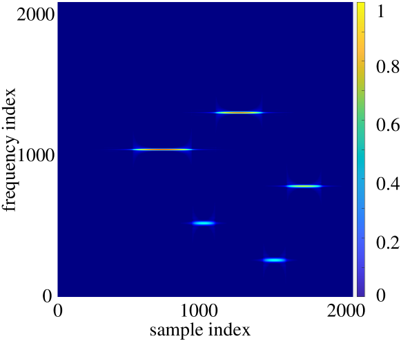
To generate the CWD-TFI, similar to [9], we capture consecutive signal samples, and assume these samples contain a complete signal pulse, and the signal pulse starts from an arbitrary point within the samples. Fig. 2 illustrates the CWD-TFI of a Costas signal with a hopping sequence of , a sub-pulse duration sequence of , a fundamental frequency of , and a starting point of . For brevity, the signal uses a Costas array to generate the FH sequence is referred to as a Costas signal. As can be seen, the CWD-TFI clearly demonstrates the time-frequency characteristic of the Costas signal by horizontal lines of different lengths and vertical positions.
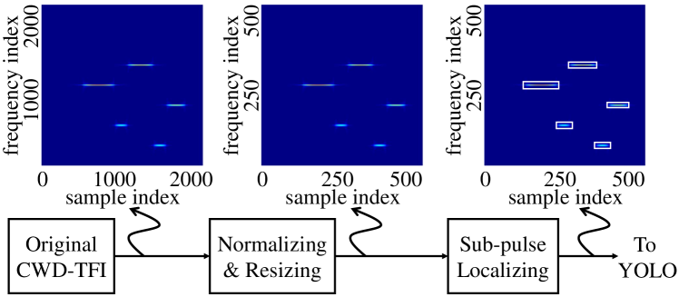
Fig. 3 shows the CWD-TFI processing procedure used to generate the input to the YOLO detection system. First, using the nearest neighbor interpolation, the CWD-TFI of pixels is resized to pixels, which is the input size of the YOLO detection system, where pixels is the width of the resized CWD-TFIs. Then, the signal sub-pulse locations in the CWD-TFI are specified by the bounding boxes (i.e., white-color rectangles in Fig. 3), as a requirement for the training of the YOLO. Note that the localization of the bounding boxes is not needed in the CWD-TFI processing procedure in the testing phase, because the bounding boxes are parts of the output of the trained YOLO detection system.
V-C “You only look once” (YOLO) Object Detection System
Among the object detection algorithm for determining the objects types and their locations in the image, YOLO [10] is well-known for its real-time detection speed, which is critical in tactical applications, such as military JRC systems. The real-time detection speed is achieved by splitting the input image into a grid of cells and predicting an object and its bounding box on each cell, instead of performing region proposal as in other object detection systems. Details of the YOLO detection system can be found in [10].
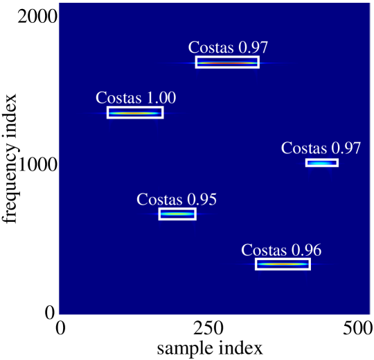
Fig. 4 shows the YOLO’s output for the CWD-TFI of a Costas signal with an FH sequence of , a sub-pulse duration sequence of , a fundamental frequency of , and a starting point of . As can be seen, the output contains not only the signal type (i.e., “Costas”) but also the locations of the signal objects (i.e., the white-color rectangular bounding boxes) and the probabilities of the detection.
V-D Data Demodulation Technique
As aforementioned, the output from the YOLO detection system contains the bounding boxes, which determine the position, horizontal, and vertical width of the signal objects in the CWD-TFI. The th left-most bounding box, corresponds to the th sub-pulse, is localized by a tuple of . Recall that for the CWD-TFI, pixels in the vertical axis correspond to a frequency range from to , while pixels in the horizontal axis correspond to a time duration of , the frequency and duration of the th sub-pulse can be calculated by
| (15) |
By comparing the combination of and values with the selections in the codebook or , the embedded symbol in each signal pulse can be determined.
It is worth noting that this demodulation technique does not require any knowledge about the channel between the JRC transceiver and the communication receiver, and hence the channel estimation is not necessary. Moreover, since our data demodulation technique is based on the CWD-TFI, its performance is not affected by the Doppler shift or timing offset between the transceiver and the communication receiver. This is because the Doppler shift or timing offset merely creates vertical or horizontal shifts of the whole set of lines, respectively. On the other hand, the shapes of the lines in the CWD-TFI remain unchanged.
VI Performance Evaluation
| Parameter | Description | Value |
|---|---|---|
| Number of sub-pulses per pulse | 5 | |
| Number of Costas array | 40 | |
| Sub-pulse duration selection set | ||
| Fundamental frequency | ||
| Resized CWD-TFI width (pixels) | 500 |
Table. I shows the parameter values used to produce the simulation results. Note that the number of Costas array is not a freely set value, but depends on , the number of sub-pulses per pulse. For instance, for . The list of available Costas arrays and their construction can be found in [6, Ch. 5]. To train the YOLO detection system, for each data embedding scheme, we generate signals with SNR ranging from dB to dB and a step size of dB. The signals are divided into a training set of signals ( of the total) and a validation set of signals (20% of the total). For the testing data, we generate signals for each embedding scheme, with SNR ranging from dB to dB and a step size of dB.
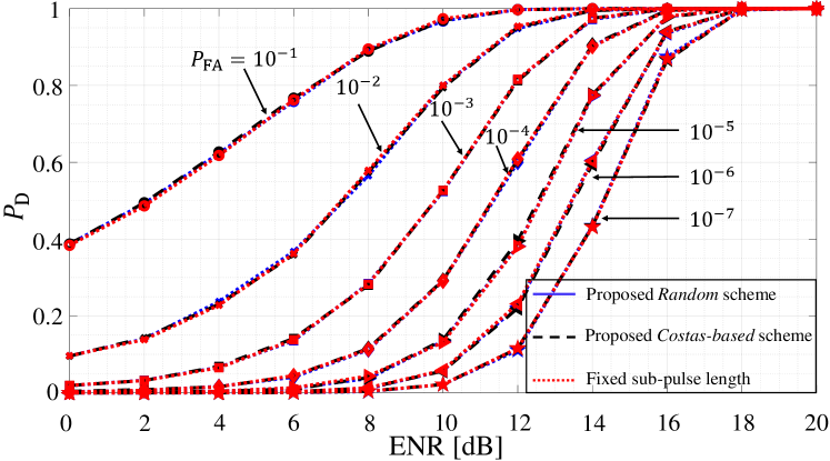
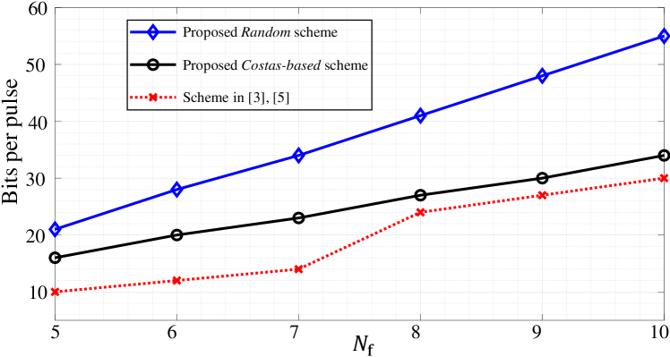
Fig. 5 shows the detection probability of the JRC sensing function for different signal waveforms (i.e., Random scheme, Costas-based scheme, and fixed sub-pulse length), , and ENR values. The results are obtained by averaging independent trials. As can be seen, for each value, the three curves almost overlap, meaning the detection probability only depends on and ENR but not the signal waveform. Therefore, varying the sub-pulse durations does not affect the detection capability of the sensing function of the FH RJC system, as long as the signal energy per each pulse is fixed.
Fig. 6 demonstrates the maximum number of bits that can be transmitted over a signal pulse of the two proposed embedding schemes and those in [3, 5]. As can be seen, the Random scheme can embed a significantly higher amount of data than the Costas-based scheme, while the Costas-based scheme can convey a slightly higher number of data bits than the scheme in [3, 5]. That is because the schemes in this paper use both sub-pulse durations and frequencies to embed signals. On the other hand, the technique in [3, 5] focuses on using antenna permutations for data embedding. Therefore, the proposed techniques are more suitable when the number of antennas is limited, while the technique in [3, 5] is suitable in the case of an extensive number of antennas is available.
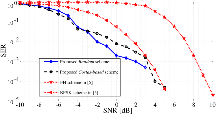
Fig. 7 illustrates the symbol error rate (SER) of the two proposed schemes and those of the techniques in [5] as functions of the signal-to-noise ratio (SNR). As can be seen, the two proposed schemes have lower SERs compared to those of the techniques in [5] for all SNRs. Distinctively, at low SNRs (i.e., dB), the two proposed schemes have similar SERs, and are about dB and dB better than those of the FH and BPSK techniques in [5], respectively. This is because the proposed techniques use the CWD, which contains the auto-correlation operation, to generate CWD-TFIs of the signals. As such, the proposed techniques are more robust against noise compared to the other techniques in [5].
VII Conclusions
We have proposed novel approaches for embedding and demodulating information bits in FH JRC systems. For data embedding, we have used both sub-pulse durations and frequencies to increase the data transmission rate. For data demodulation, to reduce the error rate, we have proposed a CWD-TFI and YOLO-based demodulation scheme that does not require channel estimation and is robust against Doppler shift and timing offset between the JRC transceiver and communication receiver. Simulation results have shown that our proposed techniques achieve higher data transmission and lower symbol error rates than the existing ones.
References
- [1] A. Hassanien, M. G. Amin, E. Aboutanios, and B. Himed, “Dual-function radar communication systems: A solution to the spectrum congestion problem,” IEEE Signal Process. Mag., vol. 36, no. 5, pp. 115–126, Sep 2019.
- [2] J. A. Zhang, F. Liu, C. Masouros, R. W. Heath, Z. Feng, L. Zheng, and A. Petropulu, “An overview of signal processing techniques for joint communication and radar sensing,” IEEE J. Sel. Topics Signal Process., vol. 69, no. 2, pp. 1295–1315, Nov 2021.
- [3] T. Huang, N. Shlezinger, X. Xu, Y. Liu, and Y. C. Eldar, “MAJoRCom: A dual-function radar communication system using index modulation,” IEEE Trans. Signal Process, vol. 68, pp. 3423–3438, May 2020.
- [4] K. Wu, J. A. Zhang, X. Huang, Y. J. Guo, and R. W. Heath, “Waveform design and accurate channel estimation for frequency-hopping MIMO radar-based communications,” IEEE Trans. on Commun., vol. 69, no. 2, pp. 1244–1258, Oct 2020.
- [5] W. Baxter, E. Aboutanios, and A. Hassanien, “Dual-function MIMO radar-communications via frequency-hopping code selection,” in Proc. Asilomar Conf. Signals, Syst., Comput. IEEE, 2018, pp. 1126–1130.
- [6] N. Levanon and E. Mozeson, Radar signals. Hoboken, NJ, USA: John Wiley & Sons, 2004.
- [7] S. M. Kay, Fundamentals of statistical signal processing: detection theory, volume II. Englewood Cliffs, NJ, USA: Prentice-Hall, 1998.
- [8] H.-I. Choi and W. J. Williams, “Improved time-frequency representation of multicomponent signals using exponential kernels,” IEEE Trans. Acoust., Speech, Signal Process., vol. 37, no. 6, pp. 862–871, Jun 1989.
- [9] L. M. Hoang, M. Kim, and S.-H. Kong, “Automatic recognition of general LPI radar waveform using SSD and supplementary classifier,” IEEE Trans. Signal Process., vol. 67, no. 13, pp. 3516–3530, May 2019.
- [10] J. Redmon, S. Divvala, R. Girshick, and A. Farhadi, “You only look once: Unified, real-time object detection,” in IEEE CVPR, 2016, pp. 779–788.