Frequency-Dependent Attenuation Reconstruction with an Acoustic Reflector
Abstract
Attenuation of ultrasound waves varies with tissue composition, hence its estimation offers great potential for tissue characterization and diagnosis and staging of pathology. We recently proposed a method that allows to spatially reconstruct the distribution of the overall ultrasound attenuation in tissue based on computed tomography, using reflections from a passive acoustic reflector. This requires a standard ultrasound transducer operating in pulse-echo mode and a calibration protocol using water measurements, thus it can be implemented on conventional ultrasound systems with minor adaptations. Herein, we extend this method by additionally estimating and imaging the frequency-dependent nature of local ultrasound attenuation for the first time. Spatial distributions of attenuation coefficient and exponent are reconstructed, enabling an elaborate and expressive tissue-specific characterization. With simulations, we demonstrate that our proposed method yields a low reconstruction error of 0.04 dB/cm at 1 MHz for attenuation coefficient and 0.08 for the frequency exponent. With tissue-mimicking phantoms and ex-vivo bovine muscle samples, a high reconstruction contrast as well as reproducibility are demonstrated. Attenuation exponents of a gelatin-cellulose mixture and an ex-vivo bovine muscle sample were found to be, respectively, 1.4 and 0.5 on average, consistently from different images of their heterogeneous compositions. Such frequency-dependent parametrization could enable novel imaging and diagnostic techniques, as well as facilitate attenuation compensation of other ultrasound-based imaging techniques.
Keywords ultrasound attenuation speed of sound computed tomography limited angle tomography
1 Introduction
Diagnostic imaging methods aim to characterize and spatially map tissue properties in order to localize and differentiate physiological and pathological structures and processes. Conventional B-mode ultrasound images echo amplitude of ultrasound, which are (longitudinal) compressional waves, reflected from local tissue features. There has also been several additional techniques derived for quantifying various tissue characteristics, using acoustic interaction phenomena and novel imaging sequences: For instance, in shear-wave elastography, focused ultrasound is used to create acoustic radiation force (a remote push) inside tissue and the local propagation speed of the resulting shear-wave is used to estimate local tissue shear-modulus [37, 14, 7]. For shear waves, amplitude decay over distance was measured to estimate shear-wave attenuation in [5], which was later studied for liver steatosis [3], liver transplantation [26], and under different preloading states [8].
Compared to the above shear-wave techniques measuring shear modulus in tissue, methods determining the propagation speed of (compressional) ultrasound waves, i.e. speed-of-sound, relate to bulk modulus in tissue, and thus have a different dependency on tissue composition [17]. The estimation of speed-of-sound distribution in tissue has been studied in various setups, e.g. in transmission mode utilizing custom made transducer architectures [13, 24] and in pulse-echo mode using conventional ultrasound scanners. For the latter, available approaches can be divided into two groups: 1) Methods that measure apparent displacements of backscattered signals insonified from different angles [35, 29, 30], and 2) Methods that use an additional passive acoustic reflector to record corresponding time-of-flight values [33]. A quantification of in-vivo speed-of-sound imaging was recently proposed for breast density [34] and sarcopenia assessment [32].
Attenuation of an ultrasound (US) wave is the result of several mechanisms: First, depending on the tissue structure dimensions, US waves may reflect or scatter at interfaces of different acoustic impedances. Viscous absorption is caused by frictious losses. In addition, a main mode of energy loss is the result of relaxation absorption, which is due to consecutive wave-fronts “hitting” the tissue that is locally recovering (bouncing back) from the push of an earlier wave-front [40]. These effects collectively lead to an overall ultrasound attenuation (UA), i.e. amplitude decay of US signals per distance they travel. Ex-vivo studies of excised tissue samples [1, 21] showed that UA differs between malignant and benign breast lesions [20] , between normal and cancerous liver [2], and between skin tissues with and without lymphedema [27]. Hence, imaging local UA-based characteristics in tissue can be a valuable diagnostic biomarker for various clinical applications.
For imaging UA, transmission mode approaches that require complex, dedicated setups were proposed, e.g. with a ring transducer for scanning the breast immersed in a water bath. Such a method proposed in [13] indicated potential for breast tumor detection and characterization. An extension of this method later in [23] using a waveform tomography approach instead of a ray based approximation of acoustic propagation further improved UA imaging accuracy. Such transmission mode setups are, however, bulky, costly, and not compatible with conventional clinical US systems with hand-held transducers, thus making UA imaging inaccessible for most clinical practice. Imaging the attenuation of compressional ultrasound waves in pulse-echo mode is non-trivial since one cannot observe the propagation of waves directly using ultrasound, unlike the slower shear-waves that can be observed using ultrasound from tissue displacements. One method for UA coefficient estimation utilizes adjacent frequency components of ultrasound signals as reference (spectra normalization) for cancelling out systemic effects such as focusing and time-gain-compensation, which then allows for an approximate derivation of the wave amplitude decay [19]. Another approach with hand-held devices is based on power spectrum measurements of backscattered echos over certain blocks [9, 11, 43, 12]. Typically a reference phantom is utilized for normalization and a (spatially weighted) regularization for reconstruction [11]. Although indicating the potential of UA in steatosis diagnosis [10], these methods rely on the assumption that UA in tissue increases linearly with frequency, which however is known not always to be the case [2].
An alternative approach of estimating the UA is with a passive reflector together with a conventional US system. An early study using such an approach for UA quantification was shown in [22, 6], which however required a-priori segmentation of imaged structures in order to only quantify piece-wise constant UA values in each structure. This is then not suitable for imaging (reconstructing) arbitrary spatial distributions of UA, and due to reconstruction instabilities, only synthetic and phantom examples could be quantified, but no actual tissue samples. Recently in [31], we proposed a novel reconstruction approach for arbitrary spatial UA distributions based on limited-angle computed tomography (LA-CT) with a conventional linear-array transducer and a passive reflector. We herein further analyze this method and extend it to also characterize the local frequency-dependence of UA. This makes our UA imaging applicable regardless of the frequency range, while providing an additional novel imaging bio-marker for tissue characterization.
2 Methods
An overview of the proposed frequency-resolved UA reconstruction procedure is schematically depicted in Fig. 1 for a simulated example.

the proposed attenuation reconstruction with the reflector setup. a) Illustration of a wide-band wavefront progression in the medium and reflection back from the passive reflector. b) Band-limited filtering of the RF echo data to obtain a single band. c) Echo amplitude along the detected wavefront for a single transmission. Reflected amplitudes for all transmit/receive channel combinations d) before and e) after calibration. f) Reconstructed UA.
Acoustic waves are emitted from a single transmit (Tx) channel and reflected from a plexiglas plate (density =, speed-of-sound =), placed at a distance from the transducer surface. Echo signals are recorded by all receive (Rx) elements in parallel and the process is repeated for each and every Tx element, such that a full-matrix (multistatic) echo dataset is obtained. A sample wide-band wavefront is illustrated in Fig. 1a at different time-points: 1) after transmission, 2) while being reflected from the passive reflector plate, 3) during echo travel, and 4) while being recorded at the transducer. The wide-band echos are then filtered to obtain band-limited signals at a defined frequency spectrum centered at frequency (Fig. 1b). Subsequently, for each single element Tx event, the band-limited echo from the upper surface of the plexiglas reflector is delineated across the Rx channels (Fig. 1c-top) and the signal envelope amplitude along this delineated reflection is derived (Fig. 1c-bottom). The reflection amplitude readings for all Tx-Rx combinations (Fig. 1d) are then calibrated (Fig. 1e), which allows to derive the attenuation distribution in the tissue specimen by solving an inverse problem (Fig. 1f). The calibration and the reconstruction procedures are explained next.
2.1 Calibration of Measurements
Refraction is the change in wavefront direction at interfaces with acoustic impedance variation, and diffraction is the bending of waves, e.g., around high impedance barriers [41]. We herein assume that the speed-of-sound and density, and hence acoustic impedance, in soft tissues vary marginally such that refraction and diffraction effects can be neglected. Accordingly, band-limited ultrasound pulses at a center frequency are assumed to propagate along rays. Note that, due to constructive and destructive interferences, acoustic intensify from a transducer element has a response as a function of wavefront (ray) propagation direction , which causes natural focusing of energy in the main beam axis as well as side lobe effects. The amplitude of the reflector for transmitting with channel and receiving with channel can then be described by
| (1) |
where is the incident-angle dependent reflection coefficient at the reflector interface, and and are, respectively, the band-limited amplitude of Tx element and the sensitivity of Rx element , at center frequency and transducer directivity . The exponent describes frequency-dependent amplitude decay based on the line integral of attenuation along rayt,r from element to .
To estimate attenuation from , any confounding factors in (1), such as transducer impulse-response influence in both and as well as reflection characteristics in , must first be compensated for. Considering the impulse response, the band-limited signals are normalized with a calibration experiment in water, where the speed-of-sound and the attenuation coefficient are known from the literature, given the water temperature and imaging frequency. By using the same predetermined frequency bandwidths and reflector distances in the water calibration as in the subsequent tissue experiments, and components can be effectively estimated and factored out. However, is still likely to differ between any calibration and application, because of the speed-of-sound mismatch between water and tissue. Such reflection coefficient changes at the acoustic reflector interface can nevertheless be analytically estimated using Snell’s law, as the wavelength () is small compared to the reflector dimensions. One can then write the reflection coefficient at the interface of the reflector and some medium ={water,tissue} as follows:
| (2) |
where speed-of-sound ratio = and density ratio =. We herein assume 1000 kg/m3 and that the speed-of-sound is dispersion-free (i.e., not frequency dependent) within the range of the utilized imaging frequency bandwidth. A normalized reflection amplitude matrix shown in Fig. 1e can then be computed with its elements corresponding to Tx and Rx being
| (3) |
Substituting (1) in (3), we can then relate calibrated and band-limited measurements at frequency to attenuation at image location (,) by
| (4) |
where the ray integral is discretized as a summation over a reconstruction grid. For this discretization, we use local attenuation value weighted by its path length within the grid element (,).
2.2 Image Reconstruction of Attenuation

Given logarithms of normalized reflection amplitudes at a specified frequency band, we perform a tomographic reconstruction of the spatial UA distribution on a spatial grid by formulating the following convex optimization problem:
| (5) |
where is the sparse ray path matrix (cf. Fig. 2) that implements (4) and is the reconstructed image at the center frequency of the band-pass filtered signal (cf. Fig. 1b). Due to the ill-conditioning of , a regularization term controlled by weight encourages spatial smoothness. Similarly to [30, 29, 33, 36], we herein use -norm for both the data and regularization terms for robustness to outliers in, respectively, the measurements and the reconstructed image (edges) [16]. Due to a lack of full angular coverage of measurements, regularization matrix implements LA-CT specific image filtering to suppress streaking artifacts orthogonal to missing projections via anisotropic weighting of directional gradients [33]. In axis-aligned directions a Sobel kernel, and in diagonal directions a Roberts kernel is used [29] (see Fig. 2d/e). Similarly to [35], we herein utilize a anisotropic weighting for a stronger regularization in the lateral direction, taking into account the uneven distribution of measurement paths. In this paper we empirically set =0.6 for all experiments , following [31]. For the numerical solution of the optimization problem (5), a limited-memory Broyden-Fletcher-Goldfarb-Shanno (L-BFGS) algorithm [4, 15, 18, 39] from the unconstrained optimization package minFunc111https://www.cs.ubc.ca/~schmidtm/Software/minFunc.html is used.
2.3 Frequency-Dependent Attenuation Reconstruction
To characterise the frequency-dependent nature of attenuation, wide-band RF echo signals are first band-pass filtered prior to reconstruction. In this work, for analyzing the echos acquired at an imaging center frequency of 5 MHz, we used MHz-bands at nominal center frequencies MHz. Band-pass filtering is herein implemented as a minimum-order filter with a stop-band attenuation of 60 dB, using the bandpass function in Matlab 2019a. For a simulated dataset, UA reconstructions at three different center frequencies are depicted in Fig. 3a.

The true center frequencies after bandpass filtering are calculated as the spectral weighted average of the filtered signal, and these used for further analysis. Note that the true center frequencies (e.g., MHz as indicated in the northwest corner of each reconstruction ) are slightly different than their nominal values (respectively MHz) used as bandpass centers. This is because the emitted wide-band pulse is approximately Gaussian with a peak at 5 Mhz, i.e. more energy is concentrated around this center. Consequently, even after a uniform filter, the resulting signals have weighted averages that are shifted towards the original peak at 5 MHz.
In Fig. 3b, the frequency-dependent attenuation values are shown for two regions, within the inclusion and outside. These plots already yield a spectral fingerprint of the attenuation characteristics in each tissue. To parametrize such spectroscopic attenuation reconstructions in a standardized way, one can assume the conventional power-law relation:
| (6) |
where attenuation is a function of frequency with medium-specific attenuation coefficient and medium-specific exponent . Accordingly, separately at each spatial image location, and are estimated by least-squares fitting the power-law function to the band-limited reconstructions, yielding the parameter maps shown in Fig. 3c and d.
Note that the attenuation term in (5) could have alternatively been replaced by the power-law equation (6), for solving all frequency bandwidths simultaneously. This could provide further robustness by regularizing reconstructions across frequencies by their expected power-law relation as well as by allowing for the direct spatial regularization of the two final parameters. However, this would also increase the optimization problem size in several folds, impeding an efficient numerical solution.
3 Experiments
Metrics. We used the following metrics for a quantitative analysis of the simulation results:
-
•
Root-mean-squared-error:
,
where represents maps of , , or , with being the number of map pixels. The ∗ and indicate, respectively, the ground-truth and our reconstruction. -
•
Contrast-ratio fraction:
,
where with mean inclusion and background values and , respectively, where the inclusion is delineated from the ground-truth map. -
•
Contrast-to-noise ratio:
,
where represents the variance.
Simulation Study. To evaluate the accuracy of frequency-dependent UA reconstructions, three simulations with different UA patterns were performed as shown in Fig.4.

The patterns were selected herein to assess inclusion separability (i.e. resolution) along and orthogonal to the tomographic projections as well as to assess positive and negative contrast inclusions with respect to a background. Acoustic propagation and received echo signals were simulated using k-Wave ultrasound simulation toolbox [42] using a spatial grid resolution of . The inclusions are simulated with a spatial variation in attenuation constant . As this toolbox does not allow to spatially vary the power-law dependence parameter , this value is kept constant at for this numerical evaluation. Full-matrix acquisition was simulated at a center frequency of with a -cycle pulse. The transducer was simulated as a linear array with 128 channels (i.e. ) with a pitch of .
Phantom and Ex-vivo Tissue Study. A tissue-mimicking gelatin phantom was prepared with 10% gelatin in water per weight. We created non-scattering and scattering phantoms; for the latter, using 1% per-weight Sigmacell Cellulose Type 50 (Sigma Aldrich, St. Louis, MO, USA). Typical for the assessment of ultrasound imaging modalities, such gelatin phantoms mimic homogeneous soft tissues with a speed-of-sound of approximately 1540 m/s, thus representative e.g. of the liver for the scattering phantom and the blood for the scatter-free one. Fresh bovine skeletal muscle was used as ex-vivo tissue samples. Using different combinations of the above, we created four phantoms listed in Table 1.
| Pht. | Inclusion | Background |
| #1 | single ex-vivo muscle | scattering gelatin |
| #2 | single ex-vivo muscle | non-scattering gelatin |
| #3 | single scattering gelatin | ex-vivo muscle |
| #4 | two non-scattering gelatin | ex-vivo muscle |
Experiments were performed with the samples submerged in distilled water at room temperature. Muscle samples were imaged with fibers oriented orthogonal to the imaging plane, to prevent potential confounding effects from anisotropic acoustic propagation along tissue fibers, as this is currently not accounted for in our model. Data acquisition was performed with a Verasonics Vantage 128-channel system connected to a Philips ATL L7-4 transducer (Verasonics, Kirkland, WA, USA). Analogous to the simulation setup, we used a wideband Tx with a center frequency of and a pulse length of cycles. The reflector distance varied from 30 mm to 46 mm depending on the sample size. For normalization of the ex-vivo/phantom amplitude matrices at a given reflector depth , we acquired calibration measurements a-priori in distilled water at room temperature at multiple reflector depths {31, 35, …,47} mm. For a given phantom measurement, we then computed the desired calibration values at via linear interpolation from the closest two calibration depths.
4 Results and Discussion
4.1 Simulation Experiments
Three simulations (#1–#3) shown in Fig. 4 were conducted (case 1 is the one illustrated earlier in Fig. 3), as representative cases with inclusions separated laterally and axially, as well with both positive and negative contrast to background. Given the ground truth maps in Fig. 4 it can be seen that the attenuation coefficient is successfully reconstructed in all cases. It is observed that with increasing UA distribution complexity (i.e., from simulation #1 to #3), the reconstruction accuracy decreases. In particular, axially-separated inclusions are reconstructed poorer compared to those laterally separated. This is due to the transmit-receive paths traversing the tissue in a mostly axial direction and hence lateral projections being missing in the resulting LA-CT, as was also reported and discussed in the context of speed-of-sound reconstruction in [31, 33]. In general, within the inclusions a shift of towards background values is observed. This is due to the lack of lateral projections combined with the regularization term in (5) axially elongating the inclusions, hence spreading them over a larger area. Since the cumulative UA effect shall stay the same, thus per-pixel inclusion values are effectively averaged with the background, inversely proportional to such artifactual area increase.
In Fig. 4 the frequency exponent -maps should not present any contrast, since the k-Wave simulated ground-truth data does not allow to spatially vary . Reconstructed -maps are seen to exhibit a deviation from such constant ground-truth value, with a fixed background offset and some artifacts along the axial edges of inclusions. The latter artifact originates from the artificial axial elongation of inclusions due to above-described LA-CT nature. This herein manifests itself stronger with increased frequency band, i.e. the higher the frequency band, the longer an inclusion axially is in the reconstruction. This effect can be observed in Fig. 3a, where the inclusion shape at MHz is axially slightly longer compared to that at MHz. This artifactually higher UA values around the axial edges at higher frequencies are then erroneously attributed by the model to increased values around these edges. Note that an inverse problem with multiple-bands formulated in the same linear system would allow to constrain and regularize the reconstructions at the parametric level (i.e. edges enforced consistently at all frequencies) and hence may prevent such axial edge artifacts in -maps.
To quantify the performance of the frequency-dependent UA reconstructions, we evaluate RMSE, CNR, and CRF for each simulation and report in Tab.LABEL:tab:sim_freqdep the average values and standard deviations over all three simulations. RMSE of is dB/cm at 1 MHz. Since ground-truth values reach up to dB/cm at 1 MHz, this demonstrates that an accurate characterization of the attenuation coefficient is possible. With an average RMSE of for , the relative estimation error with respect to the prescribed is below 6%, indicating a relatively good estimation of frequency exponent. The contrast metrics (CNR and CRF) for demonstrate that the inclusions can be successfully distinguished in reconstructions, with a contrast similar to their prescribed ground-truth value. Note that the contrast metrics are only computed for , since no contrast was prescribed for in the simulations.
| RMSE | dB/cm at 1 MHz | |
|---|---|---|
| CNR | - | |
| CRF | - |
To estimate how frequency-dependent UA imaging compares to the frequency-averaged fullband UA reconstructions [31], we compute the overall attenuation -maps using for each pixel at the known (average) transmit center frequency of 5 MHz (Fig. 5a). The corresponding fullband reconstructions are shown in Fig. 5b along with the ground-truth images derived at 5 MHz from - and -maps prescribed in the corresponding simulations (also shown in Fig. 5c). It is seen that estimating and separately, i.e. without their effects combined in the overall attenuation, improves UA characterization substantially.

This observation is corroborated by all metrics reported in Tab.3 comparatively for both methods,
| Simulation | #1 | #2 | #3 | ||
|---|---|---|---|---|---|
| RMSE | [dB/cm] | 0.28 | 0.4 | 0.58 | |
| Fullband | 0.31 | 0.52 | 0.72 | ||
| CNR | [unitless] | 5.3 | 5.7 | 1.5 | |
| Fullband | 4.0 | 2.9 | 0.3 | ||
| CRF | [%] | 77.2 | 51.8 | 31.1 | |
| Fullband | 68.8 | 34.6 | 11.2 |
where an improvement is observed in every simulated case for every metric. The average improvement in UA estimation accuracy (RMSE) is 17%, with a substantial enhancement in reconstruction contrast: an average CNR improvement of 176% and an average CRF improvement of 80%. In an actual imaging scenario such improved contrast would enable easier identification and characterization of abnormality, especially in challenging cases where more heterogeneous compositions are imaged (as in simulations and ). In comparison to a single value of frequency-averaged reconstructions, frequency-dependent UA imaging yields two biomarkers, which can either be used in independently to compensate confounding effects or in combination as a multi-parametric imaging biomarker, both of which can thus be potentially more expressive for tissue characterization.
4.2 Ex-vivo Experiments
The results of the gelatin phantom and ex-vivo experiments are shown in Fig.6

with their corresponding B-Mode images and attenuation reconstructions for the frequency-dependent (, ) parameters as well as the fullband frequency-averaged () attenuation (as in [31]). For the frequency-resolved approach, an equivalent is also computed (for comparison to [31]) based on (6) using the reconstructed coefficient and exponent maps. For the phantoms #1 & #2 with muscle inclusions in gelatin, a clear contrast is visible for all UA reconstructions (Fig.6c-f). With our proposed frequency-dependent method, it can be seen that the observed attenuation contrast originates from a variation not only in attenuation coefficient but also in frequency-dependence. For phantom #3, the reconstructed values with our proposed frequency-resolved method are consistent with phantoms #1 and #2, where the inclusion and background are inverted. Compared to the fullband method, - and -maps are seen to better preserve inclusion geometry with a reduced axial elongation, corroborating the earlier findings in the simulations. This geometric accuracy is especially important in cases, where the inclusions are not directly observable in the B-Mode images, e.g. in phantom #3 where the scattering gelatin and the surrounding muscle being isoechoic.
To suppress axial edge artifacts, especially in -maps, a possible solution would be to first delineate target regions for UA characterization and then to solve the reconstruction problem with UA constrained as piece-wise constant within each such predefined region. Such regions could be delineated manually or automatically from B-Mode images or from -maps of initial unconstrained UA reconstructions. It is also possible to reconstruct all frequency bands in a single linear system for consistent regularization and an implicit model-fitting across frequencies (e.g., to better leverage higher SNR frequencies), although this would yield much larger inverse-problems for reconstruction.
In general, the background reconstructions are seen to deteriorate towards the two lower corners, likely due to fewer tomographic projections of these regions, as also illustrated in Fig. 2c. Such errors may also propagate to the rest of the image, e.g. deteriorating how well the inclusions, especially those nearby the lower corners, are reconstructed. Consequently, phantom #4 with two inclusions on the sides yields a poorer reconstruction. Indeed, in contrast to the superior performance of the frequency-resolved method for phantoms #1–#3, for phantom #4 it yields poorer results compared to the fullband, with localization and geometry estimation errors. Surprisingly, the two inclusions with the same material are not even characterized similarly in the reconstructions of neither nor . Nevertheless, similar to the fullband representation, an attenuation map (Fig.6e) can be derived from the frequency-dependent - and -maps using (6), which is then seen to recover any lost contrast, even for phantom #4. This observation is supported quantitatively by average CNR of attenuation across ex-vivo samples being comparable as for the fullband method and using (6) from frequency-resolved parameter maps. These results also demonstrate that both our frequency-resolved and fullband methods can find applicability in different clinical scenarios.
To quantify reproducibility of our attenuation imaging and characterization for the same material in different configurations, we conducted the following analysis on the ex-vivo dataset: Since three materials in total (bovine muscle tissue, pure gelatin, and gelatin-cellulose mixture) were used in phantoms #1-#4, it is expected and desired that the same material is reconstructed as the same value across different phantoms. To quantify such consistency and constancy, in Fig.7

we compare distributions of per-pixel reconstructions within manually-delineated material regions depicted in Fig.6. We present such distributions along with the median values (red lines in Fig.7) for frequency-dependent and reconstructions as well as for fullband reconstructions. In this figure, derivation using (6) is omitted since it closely follows fullband distributions, as demonstrated earlier in Fig.6. To quantify constancy across the phantoms, we compare the median values, where their statistical distribution (mean and standard-deviation) for the same material across phantoms is reported in Table LABEL:tab:exphant.
| (Fullband) | |
|---|---|
| Muscle tissue | dB/cm |
| Gelatin+ | dB/cm |
| Gelatin | dB/cm |
| (Frequency-resolved) | |
| Muscle Tissue | dB/(MHz(0.49±0.11)cm) |
| Gelatin+ | dB/(MHz(1.36±0.12)cm) |
| Gelatin | dB/(MHz(0.83±0.51)cm) |
For the scattering gelatin with cellulose (referred as gelatin+), a low standard-deviation in Table LABEL:tab:exphant indicates a high reproducibility considering all three UA parameters (also can be observed in Fig.7b/b’/b”). Despite an expected natural tissue heterogeneity, all reconstructions of the muscular tissue also follow relatively tight distributions with somewhat similar values as seen in Figs.7a/a’/a”. Muscle tissue appears to have a high and whereas a low exponent , and accordingly presents a stark contrast to gelatin+. For the pure gelatin case, we expect an overall attenuation lower than gleatin+ due the lack of scattering that contributes to attenuation. Indeed, for phantom #2 compared to #1 & #3, both and are significantly lower, as expected, cf. Fig.7b/b”/c/c”. Interestingly, is similar with and without scattering, cf. Fig.7b’/c’. This can be explained by the fact that frequency-dependent attenuation is mostly due to relaxation and viscous absorption, and not due to scattering. Also the cellulose scatterers of size 50 m are smaller than the wavelength of the highest frequency band, thus interacting with all involved frequency bands similarly as a scattering source. Such observations unfortunately cannot be made from phantom #4, the reconstructions of which as mentioned above were affected severely by artifacts.
4.3 Extrapolation of Attenuation Characteristics
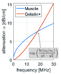
With the separate characterization of the power-law coefficients of frequency-dependent attenuation, observed attenuations can now be extrapolated to a wider hypothetical frequency range using the power-law relation (6). This is presented in Fig. 8 for the muscle and gelatin+ materials using the average values reported in Tab. LABEL:tab:exphant. From Fig. 8 we can conclude that within typical medical ultrasound bandwidth, i.e. under 20 MHz, contrast between the attenuation of these two materials would be maximized at MHz as dB/cm. Conversely, at MHz as seen in Fig. 8, the two materials will likely not exhibit any contrast at all. This demonstrates that using a frequency-averaged UA imaging, the achieved contrast may highly depend on the imaging frequency. Similarly, an imaging frequency unfit for a practical scenario may potentially lead to suboptimal tissue characterization and even potential misclassification, e.g., of a tumor. Our proposed frequency resolved attenuation imaging method redeems such limitation of having to select an optimal imaging frequency, which is likely unknown a-priori, by allowing for a characterization independent of utilized frequency range (and thus imaging transducer and frequency setting).
4.4 Further Discussion
Herein we only take the speed-of-sound difference between water calibration and target tissue into account for compensating for the reflection coefficient differences, cf. (3). Tissue speed-of-sound difference between the water calibration and target tissue may, however, also affect the angular beam profile of the transducer elements, hence confounding the assumption of amplitude matrix constancy between water and tissue in (3). Nevertheless, we believe such discrepancy of the beam profiles to be minimal, given the successful reconstruction results demonstrated with both our frequency-resolved and fullband attenuation imaging methods.
In our experiments we utilized a transmit pulse of five cycles. This could be shortened for the full spectral bandwidth of the transmit pulse to be extended up to the full transducer bandwidth, hence allowing for a wider range of reconstruction frequencies. For our purposes, within a given transducer bandwidth, either the echos from several narrowband Tx’s can be used to separately analyze the data or a single wideband Tx can be analyzed in subbands with post-processing as presented herein. Our method is thus applicable using existing US transducers and systems, provided access to raw RF data.
Similarly to most earlier works in US-CT, we herein assume a straight ray wavefront propagation, which is however only true for a constant speed-of-sound distribution. Local speed-of-sound inhomogeneities may indeed refract and aberrate wavefronts, resulting in inaccurate amplitude readings as well as the assumed wavepaths (e.g. Fig.2b) being different than actual wavepaths – both possibly leading to inaccuracies in reconstruction. A potential remedy would be to correct any ray refractions based on an a-priori speed-of-sound reconstruction, e.g. using time-of-flight measurements as in [36].
With the proposed frequency dependent UA imaging method, the opposite side of an imaged tissue needs to be accessible with a passive reflector, which limits potential anatomical regions to the breast, the extremities, male genitelia, etc. These are similar to the locations applicable for passive reflector based speed-of-sound imaging as well as for full US-CT methods. It may further be possible to use a passive reflector during open or laparoscopic surgeries, such as using a reflector with a so-called “pick-up” US transducer [38].
For a multi-parametric tissue characterization, our proposed method add s two additional imaging biomarkers complementary to robust speed-of-sound imaging methods [29, 30], which is potentially superior to elastography [17]. Hence, compared to existing ultrasound imaging modalities, a more comprehensive assessment of tissue composition and potential pathology is enabled using the proposed frequency-dependent attenuation imaging.
In addition to using the proposed attenuation imaging for diagnostic purposes, the derived UA distribution can also be utilized to improve other ultrasound imaging modalities. For instance, similarly to [30], where speed-of-sound imaging is used to correct for aberration effects in beamforming, UA maps can be used to compensate signal gain individually for each Rx-element and beamformed pixel combination. This can homogenize B-mode image appearance by removing artificial contrasts, can enhance optoacoustic [25] and functional imaging [28], and can further improve displacement estimations, e.g. in shear wave elastography.
A practical limitation of the herein proposed frequency-resolved attenuation imaging is the computational time required for the reconstructions due to the iterative numerical optimization employed. A deep variational network solution such as in [44, 45] with reconstruction times in the range of milliseconds could allow to overcome this restriction towards real-time imaging.
5 Conclusions
In this paper we have presented a novel approach for reconstructing frequency-dependent ultrasound attenuation distribution in tissue, which allows to locally characterize tissue with two biomarkers – namely the attenuation coefficient and the frequency exponent. This method allows for a more accurate reconstruction of UA distribution compared to our earlier method in [31] that reconstructs fullband frequency-averaged value of a single attenuation parameter. Our experiments with numerical simulations, tissue-mimicking gelatin phantoms, and ex-vivo tissue samples indicate a high overall reconstruction accuracy with a mean RMSE of simulated phantoms being 0.04 dB/cm at 1 MHz for attenuation coefficient and 0.08 for frequency exponent . Compared to fullband reconstructions, the frequency-dependent method offers a substantial average improvement of up to 176% in the analyzed metrics, RMSE, CNR and CRF, as reported in Table 3. Requiring only a minimal hardware add-on as a passive acoustic reflector, the proposed imaging is readily translatable to clinical applications where the opposite side of the imaged tissue region is accessible, e.g. imaging the breast, the extremities, and male genitalia.
References
- Bamber and Hill [1979] Bamber, J.C., Hill, C.R., 1979. Ultrasonic attenuation and propagation speed in mammalian tissues as a function of temperature. Ultrasound in Medicine & Biology 5, 149–157.
- Bamber and Hill [1981] Bamber, J.C., Hill, C.R., 1981. Acoustic properties of normal and cancerous human liver—i. dependence on pathological condition. Ultrasound in Medicine & Biology 7, 121–133.
- Barry et al. [2012] Barry, C.T., Mills, B., Hah, Z., Mooney, R.A., Ryan, C.K., Rubens, D.J., Parker, K.J., 2012. Shear wave dispersion measures liver steatosis. Ultrasound in Medicine & Biology 38, 175–182.
- Broyden [1970] Broyden, C.G., 1970. The Convergence of a Class of Double-rank Minimization Algorithms 1. General Considerations. IMA Journal of Applied Mathematics 6, 76–90.
- Catheline et al. [2004] Catheline, S., Gennisson, J.L., Delon, G., Fink, M., Sinkus, R., Abouelkaram, S., Culioli, J., 2004. Measurement of viscoelastic properties of homogeneous soft solid using transient elastography: An inverse problem approach. Journal of the Acoustical Society of America 116, 3734–3741.
- Chang et al. [2007] Chang, C.H., Huang, S.W., Yang, H.C., Chou, Y.H., Li, P.C., 2007. Reconstruction of ultrasonic sound velocity and attenuation coefficient using linear arrays: Clinical assessment. Ultrasound in Medicine & Biology 33, 1681–1687.
- Chintada et al. [2019] Chintada, B.R., Rau, R., Goksel, O., 2019. Acoustoelasticity analysis of shear waves for nonlinear biomechanical characterization of oil-gelatin phantoms, in: IEEE International Ultrasonics Symposium (IUS), pp. 423–426.
- Chintada et al. [2020] Chintada, B.R., Rau, R., Goksel, O., 2020. Nonlinear characterization of tissue viscoelasticity with acoustoelastic attenuation of shear-waves. arXiv:2002.12908 .
- Coila and Lavarello [2018] Coila, A.L., Lavarello, R., 2018. Regularized spectral log difference technique for ultrasonic attenuation imaging. IEEE Trans Ultrason Ferroelect Freq Contr 65, 378–389.
- Deeba et al. [2019a] Deeba, F., Ma, M., Pesteie, M., Terry, J., Pugash, D., Hutcheon, J.A., Mayer, C., Salcudean, S., Rohling, R., 2019a. Attenuation coefficient estimation of normal placentas. Ultrasound in Medicine & Biology 45, 1081–1093.
- Deeba et al. [2019b] Deeba, F., Schneider, C., Mohammed, S., Honarvar, M., Tam, E., Salcudean, S., Rohling, R., 2019b. SWTV-ACE: Spatially weighted regularization based attenuation coefficient estimation method for hepatic steatosis detection, in: Medical Image Computing and Computer Assisted Intervention (MICCAI), pp. 610–618.
- Destrempes et al. [2019] Destrempes, F., Gesnik, M., Cloutier, G., 2019. Construction of adaptively regularized parametric maps for quantitative ultrasound imaging, in: IEEE International Ultrasonics Symposium (IUS), pp. 2027–2030.
- Duric et al. [2007] Duric, N., Littrup, P., Poulo, L., Babkin, A., Pevzner, R., Holsapple, E., Rama, O., Glide, C., 2007. Detection of breast cancer with ultrasound tomography: First results with the Computed Ultrasound Risk Evaluation (CURE) prototype. Medical Physics 34, 773–785.
- Eby et al. [2013] Eby, S.F., Song, P., Chen, S., Chen, Q., Greenleaf, J.F., An, K.N., 2013. Validation of shear wave elastography in skeletal muscle. Journal of Biomechanics 46, 2381–2387.
- Fletcher [1970] Fletcher, R., 1970. A new approach to variable metric algorithms. The Computer Journal 13, 317–322.
- Fu et al. [2006] Fu, H., Ng, M.K., Nikolova, M., Barlow, J.L., 2006. Efficient minimization methods of mixed l2-l1 and l1-l1 norms for image restoration. SIAM J Sci Comput 27, 1881–1902.
- Glozman and Azhari [2010] Glozman, T., Azhari, H., 2010. A method for characterization of tissue elastic properties combining ultrasonic computed tomography with elastography. Journal of Ultrasound in Medicine 29, 387–398.
- Goldfarb [1970] Goldfarb, D., 1970. A family of variable-metric methods derived by variational means. Mathematics of Computation 24, 23–23.
- Gong et al. [2019] Gong, P., Song, P., Huang, C., Trzasko, J., Chen, S., 2019. System-independent ultrasound attenuation coefficient estimation using spectra normalization. IEEE Trans Ultrason Ferroelect Freq Contr 66, 867–875.
- Goss et al. [1978] Goss, S.A., Johnston, R.L., Dunn, F., 1978. Comprehensive compilation of empirical ultrasonic properties of mammalian tissues. The Journal of the Acoustical Society of America 64, 423–457.
- Goss et al. [1980] Goss, S.A., Johnston, R.L., Dunn, F., 1980. Compilation of empirical ultrasonic properties of mammalian tissues. II. The Journal of the Acoustical Society of America 68, 93–108.
- Huang and Li [2005] Huang, S.W., Li, P.C., 2005. Ultrasonic computed tomography reconstruction of the attenuation coefficient using a linear array. IEEE Trans Ultras Ferr Freq Control 52, 2011–2022.
- Li et al. [2017] Li, C., Sandhu, G.Y., Boone, M., Duric, N., 2017. Breast imaging using waveform attenuation tomography, in: Procs SPIE Med Imaging, p. 101390A.
- Malik et al. [2018] Malik, B., Terry, R., Wiskin, J., Lenox, M., 2018. Quantitative transmission ultrasound tomography: Imaging and performance characteristics. Medical Physics 45, 3063–3075.
- Mercep et al. [2019] Mercep, E., Herraiz, J.L., Dean-Ben, X.L., Razansky, D., 2019. Transmission–reflection optoacoustic ultrasound (TROPUS) computed tomography of small animals. Light: Science & Applications 8, 18.
- Nenadic et al. [2014] Nenadic, I.Z., Urban, M.W., Zhao, H., Sanchez, W., Morgan, P.E., Greenleaf, J.F., Chen, S., 2014. Application of attenuation measuring ultrasound shearwave elastography in 8 post-transplant liver patients, in: IEEE International Ultrasonics Symposium (IUS), pp. 987–990.
- Omura et al. [2020] Omura, M., Yoshida, K., Akita, S., Yamaguchi, T., 2020. Frequency dependence of attenuation and backscatter coefficient of ex vivo human lymphedema dermis. Journal of Medical Ultrasonics 47, 25–34.
- Rau et al. [2018] Rau, R., Kruizinga, P., Mastik, F., Belau, M., de Jong, N., Bosch, J.G., Scheffer, W., Maret, G., 2018. 3d functional ultrasound imaging of pigeons. NeuroImage 183, 469–477.
- Rau et al. [2019a] Rau, R., Schweizer, D., Vishnevskiy, V., Goksel, O., 2019a. Speed-of-sound imaging using diverging waves.
- Rau et al. [2019b] Rau, R., Schweizer, D., Vishnevskiy, V., Goksel, O., 2019b. Ultrasound aberration correction based on local speed-of-sound map estimation, in: IEEE International Ultrasonics Symposium (IUS), pp. 2003–2006.
- Rau et al. [2019c] Rau, R., Unal, O., Schweizer, D., Vishnevskiy, V., Goksel, O., 2019c. Attenuation imaging with pulse-echo ultrasound based on an acoustic reflector, in: Medical Image Computing and Computer Assisted Intervention (MICCAI), pp. 601–609.
- Sanabria et al. [2019a] Sanabria, S., Martini, K., Freystätter, G., Ruby, L., Goksel, O., Frauenfelder, T., Rominger, M.B., 2019a. Speed of sound ultrasound: a novel technique to identify muscle loss in seniors. European Radiology 29, 3–12.
- Sanabria and Goksel [2016] Sanabria, S.J., Goksel, O., 2016. Hand-held sound-speed imaging based on ultrasound reflector delineation, in: Medical Image Computing and Computer Assisted Intervention (MICCAI), pp. 568–576.
- Sanabria et al. [2018a] Sanabria, S.J., Goksel, O., Martini, K., Forte, S., Frauenfelder, T., Kubik-Huch, R.A., Rominger, M.B., 2018a. Breast-density assessment with handheld ultrasound: A novel biomarker to assess breast cancer risk and to tailor screening? European Radiology 28, 3165–3175.
- Sanabria et al. [2018b] Sanabria, S.J., Ozkan, E., Rominger, M., Goksel, O., 2018b. Spatial domain reconstruction for imaging speed-of-sound with pulse-echo ultrasound: simulation and in vivo study. Phys Med Biol 63, 215015.
- Sanabria et al. [2019b] Sanabria, S.J., Rominger, M.B., Goksel, O., 2019b. Speed-of-sound imaging based on reflector delineation. IEEE Trans Biomed Eng 66, 1949–1962.
- Sandrin et al. [2002] Sandrin, L., Tanter, M., Catheline, S., Fink, M., 2002. Shear modulus imaging with 2-D transient elastography. IEEE Trans Ultras Ferr Freq Control 49, 426–435.
- Schneider et al. [2015] Schneider, C., Nguan, C., Rohling, R., Salcudean, S., 2015. Tracked “pick-up” ultrasound for robot-assisted minimally invasive surgery. IEEE Trans Biomed Eng 63, 260–8.
- Shanno [1970] Shanno, D., 1970. Conditioning of quasi-newton methods for function minimization. Mathematics of Computation 24, 647–656.
- Smith and Webb [2011] Smith, N.B., Webb, A.G., 2011. Introduction to medical imaging: physics, engineering, and clinical applications. Cambridge Univ. Press.
- Szabo [2013] Szabo, T.L., 2013. Diagnostic Ultrasound Imaging: Inside Out. Academic Press.
- Treeby and Cox [2010] Treeby, B.E., Cox, B.T., 2010. k-Wave: MATLAB toolbox for the simulation and reconstruction of photoacoustic wave fields. J Biomed Optics 15, 021314.
- Vajihi et al. [2018] Vajihi, Z., Rosado-Mendez, I.M., Hall, T.J., Rivaz, H., 2018. Low variance estimation of backscatter quantitative ultrasound parameters using dynamic programming. IEEE Trans Ultrason Ferroelect Freq Contr 65, 2042–2053.
- Vishnevskiy et al. [2019] Vishnevskiy, V., Rau, R., Goksel, O., 2019. Deep variational networks with exponential weighting for learning computed tomography, in: Medical Image Computing and Computer Assisted Intervention (MICCAI), pp. 310–318.
- Vishnevskiy et al. [2018] Vishnevskiy, V., Sanabria, S.J., Goksel, O., 2018. Image reconstruction via variational network for real-time hand-held sound-speed imaging, in: MICCAI Workshop on Machine Learning in Medical Image Reconstruction (MLMIR), pp. 120–128.