FreeKD: Free-direction Knowledge Distillation for Graph Neural Networks
Abstract.
Knowledge distillation (KD) has demonstrated its effectiveness to boost the performance of graph neural networks (GNNs), where its goal is to distill knowledge from a deeper teacher GNN into a shallower student GNN. However, it is actually difficult to train a satisfactory teacher GNN due to the well-known over-parametrized and over-smoothing issues, leading to invalid knowledge transfer in practical applications. In this paper, we propose the first Free-direction Knowledge Distillation framework via Reinforcement learning for GNNs, called FreeKD, which is no longer required to provide a deeper well-optimized teacher GNN. The core idea of our work is to collaboratively build two shallower GNNs in an effort to exchange knowledge between them via reinforcement learning in a hierarchical way. As we observe that one typical GNN model often has better and worse performances at different nodes during training, we devise a dynamic and free-direction knowledge transfer strategy that consists of two levels of actions: 1) node-level action determines the directions of knowledge transfer between the corresponding nodes of two networks; and then 2) structure-level action determines which of the local structures generated by the node-level actions to be propagated. In essence, our FreeKD is a general and principled framework which can be naturally compatible with GNNs of different architectures. Extensive experiments on five benchmark datasets demonstrate our FreeKD outperforms two base GNNs in a large margin, and shows its efficacy to various GNNs. More surprisingly, our FreeKD has comparable or even better performance than traditional KD algorithms that distill knowledge from a deeper and stronger teacher GNN.
1. Introduction
Graph data is becoming increasingly prevalent and ubiquitous with the rapid development of the Internet, such as social networks (Hamilton et al., 2017), citation networks (Sen et al., 2008), etc. To better handle graph-structured data, graph neural networks (GNNs) provide an effective means to learn node embeddings by aggregating feature information of neighborhood nodes (Veličković et al., 2017). Because of the powerful ability in modeling relations of data, various graph neural networks have been proposed in the past decade (Kipf and Welling, 2016; Hamilton et al., 2017; Veličković et al., 2017; Chiang et al., 2019; Pei et al., 2020). The representative works include GraphSAGE (Hamilton et al., 2017), GAT (Veličković et al., 2017), GCN (Kipf and Welling, 2016), etc.
Recently, some researchers extend an interesting learning scheme, called knowledge distillation (KD) , into GNNs to further improve the performance of GNNs (Yang et al., 2020, 2021; Deng and Zhang, 2021). The basic idea among these methods is to optimize a shallower student GNN model by distilling knowledge from a deeper teacher GNN model. For instance, LSP (Yang et al., 2020) proposed a local structure preserving module to transfer the topological structure information of a GNN teacher model. The work in (Yan et al., 2020) proposed a light GNN architecture, called TinyGNN, and attempted to distill knowledge from a deep GNN teacher model to the light GNN model. GFKD (Deng and Zhang, 2021) designed a data-free knowledge distillation strategy for GNNs, enabling to transfer knowledge from a GNN teacher model by generating fake graphs.
The above methods follow the same teacher-student architecture as the traditional knowledge distillation methods (Buciluǎ et al., 2006; Hinton et al., 2015), and resort to a deeper well-optimized teacher GNN for distilling knowledge. However, when applying such an architecture to GNNs, it often suffers from the following limitations: first, it is often difficult and inefficient to train a satisfactory teacher GNN. As we know, the existing over-parameterized and over-smoothing issues often degrade the performance of the deeper GNN model. Moreover, training a deeper well-optimized model usually needs plenty of data and high computational costs. Second, according to (Yan et al., 2020; Mirzadeh et al., 2020; Yuan et al., 2021), we know that a stronger teacher model may not necessarily lead to a better student model. This may be because the mismatching of the representation capacities between a teacher model and a student model makes the student model hard to mimic the outputs of a too strong teacher model. Thus, it is difficult to find an optimal teacher GNN for a student GNN in practical applications. Considering that many powerful GNN models have been proposed in the past decade (Wu et al., 2020), this gives rise to one intuitive thought: whether we can explore a new knowledge distillation architecture to boost the performance of GNNs, avoiding the obstacle involved by training a deeper well-optimized teacher GNN?

In light of these, we propose a new knowledge distillation framework, Free-direction Knowledge Distillation based on Reinforcement learning tailored for GNNs, called FreeKD. Rather than requiring a deeper well-optimized teacher GNN for unidirectional knowledge transfer, we collaboratively learn two shallower GNNs in an effort to distill knowledge from each other via reinforcement learning in a hierarchical way. This idea stems from our observation that one typical GNN model often has better and worse performances at different nodes during training. As shown in Figure 1, GraphSAGE (Hamilton et al., 2017) has lower cross entropy losses at nodes with ID, while GAT (Veličković et al., 2017) has better performances at the rest nodes. Based on this observation, we design a free-direction knowledge distillation strategy to dynamically exchange knowledge between two shallower GNNs to benefit from each other. Considering that the direction of distilling knowledge for each node will have influence on the other nodes, we thus regard determining the directions for different nodes as a sequential decision making problem. Meanwhile, since the selection of the directions is a discrete problem, we can not optimize it by stochastic gradient descent based methods (Wang et al., 2019). Thus, we address this problem via reinforcement learning in a hierarchical way. Our hierarchical reinforcement learning algorithm consists of two levels of actions: Level 1, called node-level action, is used to distinguish which GNN is chosen to distill knowledge to the other GNN for each node. After determining the direction of knowledge transfer for each node, we expect to propagate not only the soft label of the node, but also its neighborhood relations. Thus level 2, called structure-level action, decides which of the local structures generated by our node-level actions to be propagated. One may argue that we could directly use the loss, e.g., cross entropy, to decide the directions of node-level knowledge distillation. However, this heuristic strategy only considers the performance of the node itself, but neglects its influence on other nodes, thus might lead to a sub-optimal solution. Our experimental results also verify our reinforcement learning based strategy significantly outperforms the above heuristic one.
The contributions of this paper can be summarized as:
-
•
We propose a new knowledge distillation architecture for GNNs, avoiding requiring a deeper well-optimized teacher model for distilling knowledge. The proposed framework is general and principled, which can be naturally compatible with GNNs of different architectures.
-
•
We devise a free-direction knowledge distillation strategy via a hierarchical reinforcement learning algorithm, which can dynamically manage the directions of knowledge transfer from both node-level and structure-level aspects.
-
•
Extensive experiments on five benchmark datasets demonstrate the proposed framework promotes the performance of two shallower GNNs in a large margin, and is valid to various GNNs. More surprisingly, the performance of our FreeKD is comparable to or even better than traditional KD algorithms distilling knowledge from a deeper and stronger teacher GNN.

Main architecture of FreeKD
2. Related Work
This work is related to graph neural networks, graph-based knowledge distillation, and reinforcement learning.
2.1. Graph Neural Networks
Graph neural networks have achieved promising results in processing graph data, whose goal is to learn node embeddings by aggregating nodes’ neighbor information. In recent years, lots of GNNs have been proposed (Kipf and Welling, 2016; Hamilton et al., 2017; Veličković et al., 2017). For instance, GCN (Kipf and Welling, 2016) designed a convolutional neural network architecture for graph data. GraphSAGE (Hamilton et al., 2017) proposed an efficient sample strategy to aggregate neighbor nodes. GAT (Veličković et al., 2017) applied a self-attention mechanism to GNN to assign different weights to different neighbors. SGC (Wu et al., 2019) simplified GCN by removing nonlinearities and weight matrices between consecutive convolutional layers. ROD (Zhang et al., 2021) proposed an ensemble learning based GNN model to fuse the knowledge in multiple hops. APPNP (Klicpera et al., 2018) analyzed the relationship between GCN and PageRank (Page et al., 1999), and proposed a propagation model combined with a personalized PageRank. Cluster-GCN (Chiang et al., 2019) built an efficient model based on graph clustering (Schaeffer, 2007). Being orthogonal to the above approaches developing different powerful GNN models, we concentrate on developing a new knowledge distillation framework on the basis of various GNNs.
2.2. Knowledge Distillation for GNNs
Knowledge distillation (KD) has been widely studied in computer vision (Chen et al., 2017; Liu et al., 2018), natural language processing (Kim and Rush, 2016; liu, 2019), etc. Recently, a few KD methods have proposed for GNNs. LSP (Yang et al., 2020) transferred the topological structure knowledge from a pre-trained deeper teacher GNN to a shallower student GNN. CPF (Yang et al., 2021) designed a student architecture that is a combination of a parameterized label propagation and MLP layers. GFKD (Deng and Zhang, 2021) proposed a method to generate fake graphs and distilled knowledge from a teacher GNN model without any training data involved. The authors in (Yan et al., 2020) designed an efficient GNN model by utilizing the information from peer nodes to model the local structure explicitly and distilling the neighbor structure information from a deeper GNN implicitly. The work in (Chen et al., 2021a) studied a self-distillation framework, and proposed an adaptive discrepancy retaining regularizer to empower the transferability of knowledge. RDD (Zhang et al., 2020) was a semi-supervised knowledge distillation method for GNNs. It online learnt a complicated teacher GNN model by ensemble learning, and distilled knowledge from the generated teacher model into the student model. Different from them, we focus on studying a new free-direction knowledge distillation architecture, with the purpose of dynamically exchanging knowledge between two shallower GNNs.
2.3. Reinforcement Learning
Reinforcement learning aims at training agents to make optimal decisions by learning from interactions with the environment (Arulkumaran et al., 2017). Reinforcement learning mainly has two genres (Arulkumaran et al., 2017): value-based methods and policy-based methods. Value-based methods estimate the expected reward of actions (Mnih et al., 2015), while policy-based methods take actions according to the output probabilities of the agent (Williams, 1992). There is also a hybrid of this two genres, called the actor-critic architecture (Haarnoja et al., 2018). The actor-critic architecture utilizes the value-based method as a value function to estimate the expected reward, and employs the policy-based method as a policy search strategy to take actions. Until now, reinforcement learning has been taken as a popular tool to solve various tasks, such as recommendation systems (Zheng et al., 2018), anomaly detection (Oh and Iyengar, 2019), multi-label learning (Chen et al., 2018b), etc. In this paper, we explore reinforcement learning for graph data based knowledge distillation.
3. METHODOLOGY
In this section, we elaborate the details of our FreeKD framework that is shown in Figure 2. Before introducing it, we first give some notations and preliminaries.
3.1. Preliminaries
Let denote a graph, where is the set of nodes and is the set of edge. is the feature matrix of nodes, where is the number of nodes and is the dimension of node features. Let be the feature representation of node and be its class label. The neighborhood set of node is . Currently, graph neural networks (GNNs) have become one of the most popular models for handling graph data. GNNs can learn the embedding for node at the -th layer by the following formula:
| (1) |
where is an aggregation function, and it can be defined in many forms, e.g., mean aggregator (Hamilton et al., 2017). is the learnt parameters in the -th layer of the network. The initial feature of each node can be used as the input of the first layer, i.e., .
Being orthogonal to those works developing various GNN models, our goal is to explore a new knowledge distillation framework for promoting the performance of GNNs, while addressing the issue involved because of producing a deeper teacher GNN model in the existing KD methods.
3.2. Overview of Framework
As shown in Figure 1, we observe typical GNN models often have different performances at different nodes during training. Based on this observation, we intend to dynamically exchange useful knowledge between two shallower GNNs, so as to benefit from each other. However, a challenging problem is attendant upon that: how to decide the directions of knowledge distillation for different nodes during training. To address this, we propose to manage the directions of knowledge distillation via reinforcement learning, where we regard the directions of knowledge transfer for different nodes as a sequential decision making problem (Pednault et al., 2002). Consequently, we propose a free-direction knowledge distillation framework via a hierarchical reinforcement learning, as shown in Figure 2. In our framework, the hierarchical reinforcement learning can be taken as a reinforced knowledge judge that consists of two levels of actions: 1) Level 1, called node-level action, is used to decide the distillation direction of each node for propagating the soft label; 2) Level 2, called structure-level action, is used to determine which of the local structures generated via node-level actions to be propagated.
Specifically, the reinforced knowledge judge (we call it agent for convenience) interacts with the environment constructed by two GNN models in each iteration, as in Figure 2. It receives the soft labels and cross entropy losses for a batch of nodes, and regards them as its node-level states. The agent then samples sequential node-level actions for nodes according to a learned policy network, where each action decides the direction of knowledge distillation for propagating node-level knowledge. Then, the agent receives the structure-level states and produces structure-level actions to decide which of the local structures generated on the basis of node-level actions to be propagated. After that, the two GNN models are trained based to the agent’s actions with a new loss function. Finally, the agent calculates the reward for each action to train the policy network, where the agent’s target is to maximize the expected reward. This process is repeatedly iterated until convergence.
We first give some notations for convenient presentation, before introducing how to distill both node-level and structure-level knowledge. Let and denote two GNN models, respectively. and denote the learnt representations of node obtained by and , respectively. Let and be the predicted probabilities of the two GNN models for node respectively. We regard them as the soft labels. In addition, and denote the cross entropy losses of node in and , respectively.
3.3. Agent-guided Node-level Knowledge Distillation
In this section, we introduce our reinforcement learning based strategy to dynamically distill node-level knowledge between two GNN models.
3.3.1. Node-level State
We concatenate the following features as the node-level state vector for node :
(1) Soft label vector of node in GNN .
(2) Cross entropy loss of node in GNN .
(3) Soft label vector of node in GNN .
(4) Cross entropy loss of node in GNN .
The first two kinds of features are based on the intuition that the cross entropy loss and soft label can quantify the useful knowledge for node in GNN to some extent. The last two kinds of features have the same function for . Since these features can measure the knowledge each node contains to some extent, we use them as the feature of the node-level state for predicting the node-level actions.
Formally, the state for the node is expressed as:
| (2) |
where is the concatenation operation.
3.3.2. Node-level Action
The node-level action decides the direction of knowledge distillation for node . means transferring knowledge from GNN to GNN at node , while means the distillation direction from to . If , we define node in as agent-selected node, otherwise, we define node in as agent-selected node. The actions are sampled from the probability distributions produced by a node-level policy function , where is the trainable parameters in the policy network and means the probability to take action over the state . In this paper, we adopt a three-layer MLP with the activation function as our node-level policy network.


3.3.3. Node-level Knowledge Distillation
After determining the direction of knowledge distillation for each node, the two GNN models can exchange beneficial node-level knowledge. We take Figure 3(a) as an example to illustrate our idea. In Figure 3(a), the agent-selected nodes in GNN will serve as the distilled nodes to transfer knowledge to the nodes in GNN . In the meantime, the agent-selected nodes in will be used as the distilled nodes to distill knowledge for the nodes in . In order to transfer node-level knowledge, we utilize the KL divergence to measure the distance between the soft labels of the same node in the two GNN models, and propose to minimize a new loss function for each GNN model:
| (3) | |||
| (4) |
where the value of is 0 or 1. When , we use the divergence to make the probability distribution match as much as possible, enabling the knowledge from to be transferred to at node , and vice versa for . Thus, by minimizing the two loss functions and , we can reach the goal of dynamically exchanging useful node-level knowledge between two GNN models and thus obtaining gains from each other.
3.4. Agent-guided Structure-level Knowledge Distillation
As we know, the structure information is important for graph learning. Thus, we attempt to dynamically transfer structure-level knowledge between two GNNs. It is worth noting that we don’t propagate all neighborhood information of one node as structure-level knowledge. Instead, we propagate a neighborhood subset of the node, which is comprised of agent-selected nodes. This is because we think agent-selected nodes contain more useful knowledge. We take Figure 3(b) as an example to illustrate it. is an agent-selected node in . When transferring its local structure information to , we only transfer the local structure composed of . In other words, the local structure of node we consider to transfer is made up of agent-selected nodes. We call it agent-selected neighborhood set. Moreover, considering the knowledge of the local structure in graphs is not always reliable (Zhang et al., 2020; Chen et al., 2021b), we design a reinforcement learning based strategy to distinguish which of the local structures to be propagated. Next, we introduce it in detail.
3.4.1. Structure-level State
We adopt the following features as the structure-level state vector for the local structure of node :
(1) Node-level state of node .
(2) Center similarity of node ’s agent-selected neighborhood set in the distilled network.
(3) Center similarity of the same node set as node ’s agent-selected neighborhood set in the guided network.
Since the node-level state contains much information for measuring the information of local structures, we use the node-level state as the first feature of structure-level state. As (Xie et al., 2020) points out, the center similarity can indicate the performance of GNNs, where the center similarity measures the degree of similarity between the node and its neighbors. In other words, if center similarity is high, the structure information should be more reliable. Thus, we also take center similarity as another feature. Motivated by (Xie et al., 2020), we present a similar strategy to calculate the center similarity as:
First, let and denote the agent-selected neighborhood set of node in and , respectively. Formally,
| (5) | |||
| (6) |
Then, we calculate the center similarity as:
where can be an arbitrary similarity function. Here we use the cosine similarity function . is a two-dimension vector. In order to better present what stands for, we take and in Figure 3(b) as an example. is an agent-selected node in , i.e., , and is an agent-selected node in , i.e., . For , its first element is the center similarity between and {, } in the distilled network , while its second element is the center similarity between and {, } in the guided network . Similarly, for , measures the center similarity between and {, } in , and is the center similarity between and {, } . In a word, the first element in measures the center similarity in the distilled network, and the second element measures the center similarity in the guided network.
Finally, the structure-level state for the the local structure of node is expressed as:
| (7) |
where is the concatenation operation.
3.4.2. Structure-level Action
Structure-level action is the second level action that determines which of the structure-level knowledge to be propagated. If , the agent decides to transfer the knowledge of the local structure encoded in the agent-selected neighborhood set of node , otherwise it will not be transferred. Similar to the node-level policy network, the structure-level policy network that produces structure-level actions is also comprised of a three-layer MLP with the activation function.
3.4.3. Structure-level Knowledge Distillation
We first introduce how to distill structure-level knowledge from to . The method for distilling from to is the same. First, we define the similarity between two agent-selected nodes and by:
| (8) |
where is the cosine similarity function.
To transfer structure-level knowledge, we propose a new loss function to be minimized as:
| (9) |
where and , is the size of . represents the distribution of the similarities between node and its agent-selected neighborhoods in , while represents the distribution of the similarities between node and its corresponding neighborhoods in . If the local structure of node is decided to transfer, we adopt the divergence to make match , so as to transfer structure-level knowledge. Similarly, we can propose another new loss function for distilling knowledge from to as:
| (10) |
where and , is the size of . and are defined as:
| (11) |
3.5. Optimizations
In this section, we introduce the optimization procedure of our method. The detailed training procedure is in Appendix A.1.
3.5.1. Reward
Following (Wang et al., 2019), our actions are sampled in batch, and obtain the delayed reward after two GNNs being updated according to a batch of sequential actions. Similar to (Liang et al., 2021), we utilize the performance of the models after being updated as the reward. We use the negative value of the cross entropy loss to measure the performance of the models as in (Yuan et al., 2021; Liang et al., 2021), defined as:
| (12) |
where is a hyper-parameter. is the reward for the action taken at node , and is a batch set of nodes from the training set. The reward for an action consists of two parts: The first part is the average performance for a batch of nodes, measuring the global effects that the action brings on the GNN model; The second part is the average performance of the neighborhoods of node , in order to model the local effects of .
3.5.2. Optimization for Policy Networks
Following previous studies about hierarchical reinforcement learning (Liu et al., 2021), the gradient of expected cumulative reward could be computed as follows:
| (13) |
where , is the learned parameters of the node-level policy network and structure-level policy network, respectively. Similar to (Lai et al., 2020), to speed up convergence and reduce variance , we also add a baseline reward that is the rewards at node in the last epoch. The motivation behind this is to encourage the agent to achieve better performance than that of the last epoch. Finally, we update the parameters of policy networks by gradient ascent (Williams, 1992) as:
| (14) |
where is the learning rate for reinforcement learning.
3.5.3. Optimization for GNNs
We minimize the following loss functions for optimizing and , respectively:
| (15) |
| (16) |
where , are the cross entropy losses for and , respectively. and are two node-level knowledge distillation losses. and are two structure-level distillation losses. and are two trade-off parameters.
| Cora | Chameleon | Citeseer | Texas | |||||||
| Method | Basic Model | F1 Score (Impv.) | F1 Score (Impv.) | F1 Score (Impv.) | F1 Score (Impv.) | |||||
| GCN | - | - | 85.12 | - | 33.09 | - | 75.42 | - | 57.57 | - |
| GSAGE | - | - | 85.36 | - | 48.77 | - | 76.56 | - | 76.22 | - |
| GAT | - | - | 85.45 | - | 40.29 | - | 75.66 | - | 57.84 | - |
| FreeKD | GCN | GCN | 86.53(1.41) | 86.62(1.50) | 37.61(4.52) | 37.70(4.61) | 77.28(1.86) | 77.33(1.91) | 60.28(2.71) | 60.55(2.98) |
| FreeKD | GSAGE | GSAGE | 86.41(1.05) | 86.55(1.19) | 49.89(1.12) | 49.85(1.08) | 77.78(1.22) | 77.58(1.02) | 78.76(2.54) | 77.85(1.63) |
| FreeKD | GAT | GAT | 86.46(1.01) | 86.68(1.23) | 43.96(3.67) | 44.42(4.13) | 77.13(1.47) | 77.42(1.76) | 61.18(3.34) | 61.36(3.52) |
| FreeKD | GCN | GAT | 86.65(1.53) | 86.72(1.27) | 35.58(2.49) | 43.79(3.53) | 77.39(1.97) | 77.58(1.92) | 61.06(3.49) | 60.38(2.54) |
| FreeKD | GCN | GSAGE | 86.26(1.14) | 86.76(1.40) | 35.39(2.30) | 49.89(1.12) | 77.08(1.66) | 77.68(1.12) | 60.61(3.04) | 77.58(1.36) |
| FreeKD | GAT | GSAGE | 86.67(1.22) | 86.84(1.48) | 43.96(3.67) | 49.87(1.10) | 77.24(1.58) | 77.62(1.06) | 62.45(4.61) | 78.36(2.14) |
4. EXPERIMENTS
To verify the effectiveness of our proposed FreeKD, we perform the experiments on five benchmark datasets of different domains and on GNN models of different architectures. More implementation details are given in Appendix A.3.
4.1. Experimental Setups
4.1.1. Datasets
We use five widely used benchmark datasets to evaluate our methods. Cora (Sen et al., 2008) and Citeseer (Sen et al., 2008) are two citation datasets where nodes represent documents and edges represent citation relationships. Chameleon (Rozemberczki et al., 2021) and Texas (Pei et al., 2020) are two web network datasets where nodes stand for web pages and edges show their hyperlink relationships. The PPI dataset (Hamilton et al., 2017) consists of 24 protein–protein interaction graphs, corresponding to different human tissues. In Appendix A.2, we give more information about these datasets. Following (Chen et al., 2018a) and (Huang et al., 2018), we use 1000 nodes for testing, 500 nodes for validation, and the rest for training on the Cora and Citeseer datasets. For Chameleon and Texas datasets, we randomly split nodes of each class into 60%, 20%, and 20% for training, validation and testing respectively, following (Pei et al., 2020) and (Chen et al., 2020). For the PPI dataset, we use 20 graphs for training, 2 graphs for validation, and 2 graphs for testing, as in (Chen et al., 2020). Following previous works (Veličković et al., 2017; Pei et al., 2020) , we study the transductive setting on the first four datasets, and the inductive setting on the PPI dataset. In the tasks of transductive setting, we predict the labels of the nodes observed during training, whereas in the task of inductive setting, we predict the labels of nodes in never seen graphs before.
| PPI | ||||
| Method | Basic Model | F1 Score (Impv.) | ||
| GSAGE | - | - | 69.28 | - |
| GAT | - | - | 97.30 | - |
| FreeKD | GSAGE | GSAGE | 71.72(2.44) | 71.56(2.28) |
| FreeKD | GAT | GAT | 98.79(1.49) | 98.73(1.43) |
| FreeKD | GAT | GSAGE | 98.61(1.31) | 72.39(3.11) |
4.1.2. Baselines
In the experiment, we adopt three popular GNN models, GCN (Kipf and Welling, 2016), GAT (Veličković et al., 2017), GraphSAGE (Hamilton et al., 2017), as our basic models in our method. Our framework aims to promote the performance of these GNN models. Thus, these three GNN models can be used as our baselines. Since we propose a free-direction knowledge distillation framework, we also compare with five typical knowledge distillation approaches proposed recently, including KD (Hinton et al., 2015), LSP (Yang et al., 2020), CPF (Yang et al., 2021), RDD (Zhang et al., 2020), and GNN-SD (Chen et al., 2021a), to further verify the effectiveness of our method. Following (Chen et al., 2018a; Hamilton et al., 2017), we use the Micro-F1 score as the evaluation measure throughout the experiment.
4.2. Overall Evaluations on Our Method
In this subsection, we evaluate our method using three popular GNN models, GCN (Kipf and Welling, 2016), GAT (Veličković et al., 2017), and GraphSAGE (Hamilton et al., 2017). We arbitrarily select two networks from the above three models as our basic models and , and perform our method FreeKD , enabling them to learn from each other. Note that we do not perform GCN on the PPI dataset, because of the inductive setting.
Table 1 and Table 2 report the experimental results. As shown in Table 1 and Table 2, our FreeKD can consistently promote the performance of the basic GNN models in a large margin on all the datasets. For instance, our method can achieve more than improvement by mutually learning from two GCN models on the Chameleon dataset, compared with the single GCN model. In summary, for the transductive learning tasks, our method improves the performance by 1.01% 1.97% on the Cora and Citeseer datasets and 1.08% 4.61% on the Chameleon and Texas datasets, compared with the corresponding GNN models. For the inductive learning task, our method improves the performance by 1.31% 3.11% on the PPI dataset dataset. In addition, we observe that two GNN models either sharing the same architecture or using different architectures can both benefit from each other by using our method, which shows the efficacy to various GNN models.
4.3. Comparison with Knowledge Distillation
Since our method is related to knowledge distillation, we also compare with the existing knowledge distillation methods to further verify effectiveness of our method. In this experiment, we first compare with three traditional knowledge distillation methods, KD (Hinton et al., 2015), LSP (Yang et al., 2020), CPF (Yang et al., 2021) distilling knowledge from a deeper and stronger teacher GCNII model (Chen et al., 2020) into a shallower student GAT model. The structure details of GCNII and GAT could be found in the Appendix A.3. In addition, we also compare with an ensemble learning method, RDD (Zhang et al., 2020), where a complex teacher network is generated by ensemble learning for distilling knowledge. Finally, we take GNN-SD (Chen et al., 2021a) as another baseline, which distills knowledge from shallow layers into deep layers in one GNN. For our FreeKD, we take two GAT sharing the same structure as the basic models.
Table 3 lists the experimental results. Surprisingly, our FreeKD perform comparably or even better than the traditional knowledge distillation methods (KD, LSP, CPF) on all the datasets. This demonstrates the effectiveness of our method, as they distill knowledge from the stronger teacher GCNII while we only mutually distill knowledge between two shallower GAT. In addition, our FreeKD consistently outperforms GNN-SD and RDD, which further illustrates the effectiveness of our proposed FreeKD.
| Cora | Chameleon | Citeseer | Texas | PPI | |
| Teacher | 87.80 | 46.79 | 78.60 | 65.14 | 99.41 |
| GCNII | |||||
| KD | 86.13 | 43.69 | 77.03 | 59.46 | 97.81 |
| LSP | 86.25 | 44.01 | 77.21 | 59.73 | 98.25 |
| CPF | 86.41 | 41.40 | 77.80 | 60.81 | - |
| GNN-SD | 85.75 | 40.79 | 75.96 | 58.65 | 97.73 |
| RDD | 85.84 | 41.15 | 76.02 | 58.92 | 97.66 |
| FreeKD | 86.68 | 44.42 | 77.42 | 61.36 | 98.79 |


4.4. Ablation Study
We perform ablation study to verify the effectiveness of the components in our method. We use GCN as the basic models and in our method, and conduct the experiments on two datasets of different domains, Chameleon and Cora. When setting , this means that we only transfer the node-level knowledge. We denote it FreeKD-node for short. To evaluate our reinforcement learning based node judge module, we design three variants:
-
•
FreeKD-w.o.-judge: our FreeKD without using the agent. and distills knowledge for each node from each other.
-
•
FreeKD-loss: our FreeKD without using the reinforced knowledge judge. It determines the directions of knowledge distillation only relying on the cross entropy loss.
-
•
FreeKD-all-neighbors: our FreeKD selecting the directions of node-level knowledge distillation via node-level actions, but using all neighborhood nodes as the local structure.
-
•
FreeKD-all-structures: our FreeKD selecting the directions of node-level knowledge distillation, but without using structure-level actions for structure-level knowledge distillation.
Table 4 shows the results. FreeKD-node is better than GCN, showing that mutually transferring node-level knowledge via reinforcement learning is useful for boosting the performance of GNNs. FreeKD obtain better results than FreeKD-node. It illustrates distilling structure knowledge by our method is beneficial to GNNs. FreeKD achieves better performance than FreeKD-w.o.-judge, illustrating dynamically determining the knowledge distillation direction is important. In addition, FreeKD outperforms FreeKD-loss. This shows that directly using the cross entropy loss to decide the directions of knowledge distillation is sub-optimal. As stated before, this heuristic strategy only considers the performance of the node itself, but neglects the influence of the node on other nodes. Additionally, FreeKD has superiority over FreeKD-all-neighbors, demonstrating that transferring part of neighborhood information selected by our method is more effective than transferring all neighborhood information for GNNs. Finally, FreeKD obtains better performance than FreeKD-all-structures, which indicates our reinforcement learning based method can transfer more reliable structure-level knowledge. In summary, these results demonstrate our proposed knowledge distillation framework with a hierarchical reinforcement learning strategy is effective.
| Chameleon | Cora | |||||
| Method | Network | F1 Score | F1 Score | |||
| GCN | - | - | 33.09 | - | 85.12 | - |
| FreeKD-node | GCN | GCN | 36.35 | 36.42 | 86.17 | 86.03 |
| FreeKD-w.o.-judge | GCN | GCN | 35.33 | 35.27 | 85.83 | 85.76 |
| FreeKD-loss | GCN | GCN | 35.86 | 35.79 | 85.89 | 85.97 |
| FreeKD-all-neighbors | GCN | GCN | 36.85 | 36.73 | 86.21 | 86.26 |
| FreeKD-all-structures | GCN | GCN | 36.53 | 36.62 | 86.13 | 86.07 |
| FreeKD | GCN | GCN | 37.61 | 37.70 | 86.53 | 86.62 |
4.5. Visualizations
We further intuitively show the effectiveness of the reinforced knowledge judge to dynamically decide the directions of knowledge distillation. We set GCN as and GraphSAGE as , and train our FreeKD on the Cora dataset. Then, we poison by adding random Gaussian noise with a standard deviation to its model parameters. Finally, we visualize the agent’s output, i.e., node-level policy probabilities and at node for and , respectively. To better visualize, we show a subgraph composed of the first 30 nodes and their neighborhoods.
Figure 4 shows the results using different standard deviations . In Figure 4 (a), (b), and (c), the higher the probability output by the agent is, the redder the node is. And this means that the probability for the node in this network to serve as a distilled node to transfer knowledge to the corresponding node of the other network is higher. As shown in Figure 4 (a), when without adding noise, the degrees of the red color in and are comparable. As the noise is gradually increased in , the red color becomes more and more light in , but an opposite case happens in , as shown in Figure 4 (b) and (c). This is because the noise brings negative influence on the outputs of the network, leading to inaccurate soft labels and large losses. In such a case, our agent can output low probabilities for the network . Thus, our agent can effectively determine the direction of knowledge distillation for each node.
| Dataset | Network | =0.0 | =0.1 | =0.3 | =0.5 | =0.7 | =0.9 | |
| Cora | GCN | GCN | 86.32 | 86.39 | 86.57 | 86.31 | 86.12 | 85.23 |
| GAT | GAT | 86.21 | 86.45 | 86.41 | 86.57 | 86.32 | 86.22 | |
4.6. Sensitivity and Convergence Analysis
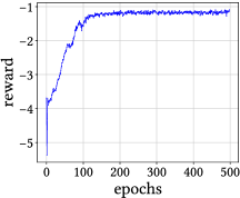
In our method, there are three main hyper-parameters, i.e., in the reward function (12), and in the loss function (15) and (16). We study the sensitivity of our method to these hyper-parameters on the Cora dataset. First, we investigate the impact of in the agent’s reward function on the performance of our method. As shown in Table 5, with the values of increasing, the performance of our method will fall after rising. In the meantime, our method is not sensitive to in a relatively large range. We also study the parameter sensitiveness of our method to and . Figure 5(a) shows the results. Our method is still not sensitive to these two hyper-parameters in a relatively large range. Additionally, we analyze the convergence of our method. Figure 5(b) shows the reward convergence curve. Our method is convergent after 100 epochs.

5. Conclusion
In this paper, we proposed a free-direction knowledge distillation framework to enable two shallower GNNs to learn from each other, without requiring a deeper well-optimized teacher GNN. Meanwhile, we devised a hierarchical reinforcement learning mechanism to manage the directions of knowledge transfer, so as to distill knowledge from both node-level and structure-level aspects. Extensive experiments demonstrated the effectiveness of our method.
Acknowledgements.
This work was supported by the National Natural Science Foundation of China (NSFC) under Grants 62122013, U2001211.References
- (1)
- liu (2019) 2019. Improving multi-task deep neural networks via knowledge distillation for natural language understanding. arXiv (2019).
- Arulkumaran et al. (2017) Kai Arulkumaran, Marc Peter Deisenroth, Miles Brundage, and Anil Anthony Bharath. 2017. Deep reinforcement learning: A brief survey. IEEE Signal Processing Magazine 34, 6 (2017), 26–38.
- Buciluǎ et al. (2006) Cristian Buciluǎ, Rich Caruana, and Alexandru Niculescu-Mizil. 2006. Model compression. In KDD. 535–541.
- Chen et al. (2021b) Deli Chen, Yankai Lin, Guangxiang Zhao, Xuancheng Ren, Peng Li, Jie Zhou, and Xu Sun. 2021b. Topology-Imbalance Learning for Semi-Supervised Node Classification. NeurIPS (2021).
- Chen et al. (2017) Guobin Chen, Wongun Choi, Xiang Yu, Tony Han, and Manmohan Chandraker. 2017. Learning efficient object detection models with knowledge distillation. NeurIPS (2017).
- Chen et al. (2018a) Jie Chen, Tengfei Ma, and Cao Xiao. 2018a. Fastgcn: fast learning with graph convolutional networks via importance sampling. (2018).
- Chen et al. (2020) Ming Chen, Zhewei Wei, Zengfeng Huang, Bolin Ding, and Yaliang Li. 2020. Simple and deep graph convolutional networks. In ICML. 1725–1735.
- Chen et al. (2018b) Tianshui Chen, Zhouxia Wang, Guanbin Li, and Liang Lin. 2018b. Recurrent attentional reinforcement learning for multi-label image recognition. In AAAI.
- Chen et al. (2021a) Yuzhao Chen, Yatao Bian, Xi Xiao, Yu Rong, Tingyang Xu, and Junzhou Huang. 2021a. On self-distilling graph neural network. In IJCAI. 2278–2284.
- Chiang et al. (2019) Wei-Lin Chiang, Xuanqing Liu, Si Si, Yang Li, Samy Bengio, and Cho-Jui Hsieh. 2019. Cluster-gcn: An efficient algorithm for training deep and large graph convolutional networks. In KDD. 257–266.
- Deng and Zhang (2021) Xiang Deng and Zhongfei Zhang. 2021. Graph-Free Knowledge Distillation for Graph Neural Networks. (2021).
- Haarnoja et al. (2018) Tuomas Haarnoja, Aurick Zhou, Pieter Abbeel, and Sergey Levine. 2018. Soft actor-critic: Off-policy maximum entropy deep reinforcement learning with a stochastic actor. In ICML. 1861–1870.
- Hamilton et al. (2017) William L Hamilton, Rex Ying, and Jure Leskovec. 2017. Inductive representation learning on large graphs. In NeurIPS. 1025–1035.
- Hinton et al. (2015) Geoffrey Hinton, Oriol Vinyals, Jeff Dean, et al. 2015. Distilling the knowledge in a neural network. arXiv 2, 7 (2015).
- Huang et al. (2018) Wenbing Huang, Tong Zhang, Yu Rong, and Junzhou Huang. 2018. Adaptive sampling towards fast graph representation learning. (2018).
- Kim and Rush (2016) Yoon Kim and Alexander M Rush. 2016. Sequence-level knowledge distillation. arXiv (2016).
- Kingma and Ba (2014) Diederik P Kingma and Jimmy Ba. 2014. Adam: A method for stochastic optimization. (2014).
- Kipf and Welling (2016) Thomas N Kipf and Max Welling. 2016. Semi-supervised classification with graph convolutional networks. arXiv (2016).
- Klicpera et al. (2018) Johannes Klicpera, Aleksandar Bojchevski, and Stephan Günnemann. 2018. Predict then propagate: Graph neural networks meet personalized pagerank. arXiv (2018).
- Lai et al. (2020) Kwei-Herng Lai, Daochen Zha, Kaixiong Zhou, and Xia Hu. 2020. Policy-gnn: Aggregation optimization for graph neural networks. In KDD. 461–471.
- Liang et al. (2021) Shining Liang, Ming Gong, Jian Pei, Linjun Shou, Wanli Zuo, Xianglin Zuo, and Daxin Jiang. 2021. Reinforced Iterative Knowledge Distillation for Cross-Lingual Named Entity Recognition. In KDD. 3231–3239.
- Liu et al. (2021) Yaoyao Liu, Bernt Schiele, and Qianru Sun. 2021. RMM: Reinforced Memory Management for Class-Incremental Learning. NeurIPS (2021).
- Liu et al. (2018) Yongcheng Liu, Lu Sheng, Jing Shao, Junjie Yan, Shiming Xiang, and Chunhong Pan. 2018. Multi-label image classification via knowledge distillation from weakly-supervised detection. In MM. 700–708.
- Mirzadeh et al. (2020) Seyed Iman Mirzadeh, Mehrdad Farajtabar, Ang Li, Nir Levine, Akihiro Matsukawa, and Hassan Ghasemzadeh. 2020. Improved knowledge distillation via teacher assistant. In AAAI. 5191–5198.
- Mnih et al. (2015) Volodymyr Mnih, Koray Kavukcuoglu, David Silver, Andrei A Rusu, Joel Veness, Marc G Bellemare, Alex Graves, Martin Riedmiller, Andreas K Fidjeland, Georg Ostrovski, et al. 2015. Human-level control through deep reinforcement learning. nature 518, 7540 (2015), 529–533.
- Oh and Iyengar (2019) Min-hwan Oh and Garud Iyengar. 2019. Sequential anomaly detection using inverse reinforcement learning. In KDD. 1480–1490.
- Page et al. (1999) Lawrence Page, Sergey Brin, Rajeev Motwani, and Terry Winograd. 1999. The PageRank citation ranking: Bringing order to the web. Technical Report. Stanford InfoLab.
- Pednault et al. (2002) Edwin Pednault, Naoki Abe, and Bianca Zadrozny. 2002. Sequential cost-sensitive decision making with reinforcement learning. In KDD. 259–268.
- Pei et al. (2020) Hongbin Pei, Bingzhe Wei, Kevin Chen-Chuan Chang, Yu Lei, and Bo Yang. 2020. Geom-gcn: Geometric graph convolutional networks. (2020).
- Rozemberczki et al. (2021) Benedek Rozemberczki, Carl Allen, and Rik Sarkar. 2021. Multi-scale attributed node embedding. Journal of Complex Networks 9, 2 (2021), cnab014.
- Schaeffer (2007) Satu Elisa Schaeffer. 2007. Graph clustering. Computer Science Review 1, 1 (2007), 27–64.
- Sen et al. (2008) Prithviraj Sen, Galileo Namata, Mustafa Bilgic, Lise Getoor, Brian Galligher, and Tina Eliassi-Rad. 2008. Collective classification in network data. AI Magazine 29, 3 (2008), 93–93.
- Veličković et al. (2017) Petar Veličković, Guillem Cucurull, Arantxa Casanova, Adriana Romero, Pietro Lio, and Yoshua Bengio. 2017. Graph attention networks. arXiv preprint arXiv:1710.10903 (2017).
- Wang et al. (2019) Bo Wang, Minghui Qiu, Xisen Wang, Yaliang Li, Yu Gong, Xiaoyi Zeng, Jun Huang, Bo Zheng, Deng Cai, and Jingren Zhou. 2019. A minimax game for instance based selective transfer learning. In KDD. 34–43.
- Williams (1992) Ronald J Williams. 1992. Simple statistical gradient-following algorithms for connectionist reinforcement learning. Machine learning 8, 3 (1992), 229–256.
- Wu et al. (2019) Felix Wu, Amauri Souza, Tianyi Zhang, Christopher Fifty, Tao Yu, and Kilian Weinberger. 2019. Simplifying graph convolutional networks. In ICML. 6861–6871.
- Wu et al. (2020) Zonghan Wu, Shirui Pan, Fengwen Chen, Guodong Long, Chengqi Zhang, and S Yu Philip. 2020. A comprehensive survey on graph neural networks. IEEE Transactions on Neural Networks and Learning Systems 32, 1 (2020), 4–24.
- Xie et al. (2020) Yiqing Xie, Sha Li, Carl Yang, Raymond Chi Wing Wong, and Jiawei Han. 2020. When do gnns work: Understanding and improving neighborhood aggregation. In IJCAI.
- Yan et al. (2020) Bencheng Yan, Chaokun Wang, Gaoyang Guo, and Yunkai Lou. 2020. TinyGNN: Learning Efficient Graph Neural Networks. In KDD. 1848–1856.
- Yang et al. (2021) Cheng Yang, Jiawei Liu, and Chuan Shi. 2021. Extract the Knowledge of Graph Neural Networks and Go Beyond it: An Effective Knowledge Distillation Framework. In WWW. 1227–1237.
- Yang et al. (2020) Yiding Yang, Jiayan Qiu, Mingli Song, Dacheng Tao, and Xinchao Wang. 2020. Distilling knowledge from graph convolutional networks. In CVPR. 7074–7083.
- Yuan et al. (2021) Fei Yuan, Linjun Shou, Jian Pei, Wutao Lin, Ming Gong, Yan Fu, and Daxin Jiang. 2021. Reinforced multi-teacher selection for knowledge distillation. In AAAI, Vol. 35. 14284–14291.
- Zhang et al. (2021) Wentao Zhang, Yuezihan Jiang, Yang Li, Zeang Sheng, Yu Shen, Xupeng Miao, Liang Wang, Zhi Yang, and Bin Cui. 2021. ROD: reception-aware online distillation for sparse graphs. In KDD. 2232–2242.
- Zhang et al. (2020) Wentao Zhang, Xupeng Miao, Yingxia Shao, Jiawei Jiang, Lei Chen, Olivier Ruas, and Bin Cui. 2020. Reliable data distillation on graph convolutional network. In SIGMOD. 1399–1414.
- Zheng et al. (2018) Guanjie Zheng, Fuzheng Zhang, Zihan Zheng, Yang Xiang, Nicholas Jing Yuan, Xing Xie, and Zhenhui Li. 2018. DRN: A deep reinforcement learning framework for news recommendation. In WWW. 167–176.
Appendix A APPENDIX
To support the reproducibility of our work, we introduce more details about training and experiments in the appendix.
A.1. Training procedure
Algorithm 1 is the pseudo-code of the our FreeKD training procedure. The GNNs and the agent closely interact with each other when training. For each batch, we first calculate the cross entropy loss for training GNNs. The node-level states for a batch of nodes are then calculated and feed into the node-level policy network. After that, we sample node-level actions from the policy probabilities produced by the agent to decide the directions of knowledge distillation between two GNNs. Then, the agent receives structure-level states from environment and produces structure-level actions to decide which of the local structures to be propagated. The two-level states and actions are stored in the history buffer. Next, we train the two GNNs with the overall loss. After that, for the stored states and actions, we calculate the delayed rewards according to the performance of GNNs and update the policy network with gradient ascent. The GNNs and the agent are learned together and mutually improved.
A.2. Datasets Description and Statistics
In our experiments, we use five widely used public datasets of different domains to evaluate our method. Table 6 summarizes the statistics of the five datasets. In the following we introduce more information about these five datasets.
Cora (Sen et al., 2008) and Citeseer (Sen et al., 2008) are two citation networks. Cora is composed of papers in the machine learning domain, and Citeseer is about computer science publications. In these two datasets, nodes stand for documents while edges represent the citation relationship between documents. The node feature is the bag-of-words representation of document and the node label is the corresponding research domain.
Chameleon (Rozemberczki et al., 2021) and Texas (Pei et al., 2020) are two web networks. In these two datasets, the nodes represent web pages and the edges are the hyperlinks between web pages. The node feature is the bag-of-words vector that represents the corresponding web page and the node label is its corresponding category.
PPI (Hamilton et al., 2017) describes the protein-protein interactions in human tissues. PPI is a widely used inductive learning dataset, containing 24 protein-protein interactions graphs. Every graph is about a specific human tissue. PPI takes positional gene sets, motif gene sets and immunological signatures as the node feature, and takes the corresponding gene ontology set as the node label.
| Dataset | # Graphs | # Nodes | # Edges | # Features | # Classes |
| Cora | 1 | 2708 | 5429 | 1433 | 7 |
| Citeseer | 1 | 3327 | 4732 | 3703 | 6 |
| Chameleon | 1 | 2277 | 36101 | 2325 | 4 |
| Texas | 1 | 183 | 309 | 1703 | 5 |
| PPI | 24 | 56944 | 818716 | 50 | 121 |
A.3. Implementation Details
All the results are averaged above 10 times and we run our experiments on GeForce RTX 2080 Ti GPU. We use the Adam optimizer (Kingma and Ba, 2014) for training and adopt early stopping with a patience on validation sets of epochs. The initial learning rate is for GAT and for GCN, GraphSAGE, and is decreased by multiplying every epochs. For the reinforced knowledge judge module, we set a fixed learning rate of . We set the dropout rate to and the norm regularization weight decay to . The parameters of all GNN models are randomly initialized. The hyper-parameters and in our method are searched from , and is searched from . The node-level policy network and structure-level policy network are both 3-layer MLP with tanh activation function and the size of hidden layer is set to . For the transductive setting, the number of layers in GNNs is set to and the hidden size is set to . For the inductive setting, the number of layers in GNNs is set to and the hidden size is set to . For GAT, the attention dropout probability is set to and the number of attention heads is set to . For GraphSAGE, we use the mean aggregator to sample neighbors.
In the experiments of comparison with other knowledge distillation methods, the student model, i.e., GAT, is set to 2-layer with 64 hidden size in the transductive setting and 3-layer with 256 hidden size in the inductive setting. For the teacher model GCNII, the number of layers is set to and the hidden size is set to in the transductive setting; in the inductive setting, the number of layers is set to and the hidden size is set to . For all the compared knowledge distillation methods, we use the parameters as their original papers suggest and report their best results.