Free Groups as End Homogeneity Groups of -manifolds
Abstract.
For every finitely generated free group , we construct an irreducible open -manifold whose end set is homeomorphic to a Cantor set, and with the end homogeneity group of isomorphic to . The end homogeneity group is the group of all self-homeomorphisms of the end set that extend to homeomorphisms of the entire -manifold. This extends an earlier result that constructs, for each finitely generated abelian group , an irreducible open -manifold with end homogeneity group . The method used in the proof of our main result also shows that if is a group with a Cayley graph in such that the graph automorphisms have certain nice extension properties, then there is an irreducible open -manifold with end homogeneity group .
Key words and phrases:
Open 3-manifold, rigidity, manifold end, geometric index, Cantor set, homogeneity group, abelian group, defining sequence2010 Mathematics Subject Classification:
Primary 54E45, 57M30, 57N12; Secondary 57N10, 54F65Introduction
Each compact set in (or in ) has for its complement an open -manifold . There is often a close relation between properties of the embedding of in and properties of this -manifold complement. Consider, for example, embeddings of knots and the study of knot complements. See also [21] for a construction of a Cantor set with hyperbolic complement.
If the compact set is a Cantor set in , then the complement of is an open -manifold with end set . The embedding of the Cantor set gives rise to properties of the corresponding complementary -manifold and of the end set of . See [9, 11, 21] for examples of this. There has been extensive study of embeddings of Cantor sets in or . The space of embeddings is extremely complicated. See for example [15].
In [10], the authors showed that for every finitely generated abelian group , there is an irreducible open 3-manifold with end homogeneity group isomorphic to . The end homogeneity group is the group of all end homeomorphisms that extend to the entire 3-manifold. This -manifold is the complement of a carefully constructed Cantor set associated with in .
For further examples of properties of embeddings related to properties of the containing 3-manifold or of the 3-manifold arising as the complement, see [16] for a relation of certain group presentations to certain wild embeddings of arcs and [6] for a construction of certain wild Cantor sets that are Julia sets. See also [14] for another example of the use of embeddings to construct certain 3-manifolds.
In this paper, the authors show that for any finitely generated free group , there is an irreducible open 3-manifold with the end homogeneity group . The proof leads to a technique which shows that if a group has a Cayley graph embeddable in in a particularly nice way, then there is an irreducible open 3-manifold with the end homogeneity group isomorphic to .
In Section 1 we discuss concepts and results needed in the paper. This includes the concepts of geometric index, local genus, embedding homogeneity groups, end homogeneity groups, Antoine Cantor sets, and rigidly embedded Cantor sets. In Section 2, we carefully construct a specific Cayley graph in for the free group on generators, . In Section 3 we construct a specific Cantor set in related to the Cayley graph constructed in Section 2. In Section 4 we prove the main theorems. We end with some open questions.
1. Preliminaries
Background Information
We refer to [12, 13, 8, 11] for a discussion of Cantor sets in general and of rigid Cantor sets, and to [24] for results about local genus of points in Cantor sets and defining sequences for Cantor sets. The bibliographies in these papers contain additional references to results about Cantor sets. Two Cantor sets and in (or ) are said to be equivalent or equivalently embedded if there is a self-homeomorphism of (or ) taking to . If there is no such homeomorphism, the Cantor sets are said to be inequivalent, or inequivalently embedded. A Cantor set is said to be rigidly embedded in (or ) if the only self-homeomorphism of that extends to a homeomorphism of (or ) is the identity.
Geometric Index
We list the results which we will need on geometric index. See Schubert [17, 8] for more details. If is a link in the interior of a solid torus , the geometric index of in , denoted by , is the minimum of over all meridional disks of intersecting transversely. If is a solid torus and is a finite union of disjoint solid tori so that , then the geometric index of in is where is a core of .
Note: An unknotted solid torus is a solid torus with center line an unknotted circle in .
Theorem 1.1.
Theorem 1.2.
There is one additional result we will need.
Defining Sequences and Local Genus
We review the definition and some basic facts from [24] about the local genus of points in a Cantor set. Also see [24] for a discussion of defining sequences.
A defining sequence for a Cantor set in is a properly nested sequence of handlebodies such that . Let be the set of all defining sequences for a Cantor set . Let be one of these defining sequences. For , denote by the union of those components of which intersect . Define
where is the genus of . The number is called the genus of the Cantor set with respect to the subset . For we call the number the local genus of the Cantor set at the point and denote it by .
Remark 1.4.
The genus measures the minimum genus of handlebodies needed in any defining sequence for the Cantor set. The standard Cantor set has genus at each point since it can be defined as an intersection of genus balls. An Antoine Cantor set (illustrated in Figure 1) has genus 1 at each point since it is defined by genus 1 manifolds (solid tori), but cannot be defined by genus 0 manifolds (balls).
Remark 1.5.
Let be an arbitrary point of a Cantor set and a homeomorphism. Then the local genus is the same as the local genus . Also note that if , then the local genus of in is less than or equal to the local genus of in . See [24, Theorem 2.4].
The following result from [24] is needed to show that certain points in our examples have local genus .
Theorem 1.6.
[24] Let be Cantor sets and . Suppose there exists a 3-ball and a 2-disc such that
-
(1)
, , ; and
-
(2)
and where and are the components of .
Then .
Embedding Homogeneity Groups and End Homogeneity Groups
For background on Freudenthal compactifications and theory of ends, see [4, 7, 20]. For an alternate proof using defining sequences of the result that every homeomorphism of the open -manifold extends to a homeomorphism of its Freudenthal compactification, see [9].
Each Cantor set in has for its complement an open -manifold with end set . The embedding of the Cantor set gives rise to properties of the corresponding complementary -manifold . See [9, 11, 21] for examples of this.
We investigate possible group actions on the end set of the open -manifold in the following sense: The homogeneity group of the end set is the group of homeomorphisms of the end set that extend to homeomorphisms of the open -manifold . Referring specifically to the embedding of the Cantor set, this group can also be called the embedding homogeneity group of the Cantor set. See [5, 22] for a discussion and overview of some other types of homogeneity.
The standardly embedded Cantor set is at one extreme here. The embedding homogeneity group is the full group of self-homeomorphisms of the Cantor set, an extremely rich group (there is such a homeomorphism taking any countable dense subset to any other). Cantor sets with this full embedding homogeneity group are called strongly homogeneously embedded. See Daverman [3] for an example of a non-standard Cantor set with this property.
At the other extreme are rigidly embedded Cantor sets, i.e. those Cantor sets for which only the identity homeomorphism extends. Shilepsky [19] constructed Antoine type [2] rigid Cantor sets. Their rigidity is a consequence of Sher’s result [18] that if two Antoine Cantor sets are equivalently embedded, then the stages of their defining sequences must match up exactly. Newer examples [13, 8] of non-standard Cantor sets were constructed that are both rigidly embedded and have simply connected complement. See [23] for additional examples of rigidity.
These examples naturally lead to the question of which types of groups can arise as end homogeneity groups between the two extremes mentioned above. In this paper we show that for each finitely generated free group , there is an irreducible open 3-manifold with the end set homeomorphic to a Cantor set and with the end homogeneity group isomorphic to .
Remark 1.7.
The Cantor sets produced are unsplittable as are the set of ends, in the sense that no -sphere separates points of the Cantor set (respectively, points of the end set). Correspondingly, the complements of the Cantor sets produced are irreducible in the sense that every 2-sphere in the complement bounds a 3-ball.
Antoine Cantor Sets
An Antoine Cantor set is described as follows. Let be an unknotted solid torus in . Let be a chain of at least four linked, pairwise disjoint, unknotted solid tori in as in Figure 1. Inductively, consists of pairwise disjoint solid tori in and is obtained from by placing a chain of at least four linked, pairwise disjoint, unknotted solid tori in each component of . If the diameter of the components goes to , the Antoine Cantor set is .

We refer to Sher’s paper [18] for basic results and description of Antoine Cantor sets. The key result we will need is the following:
Theorem 1.8.
[18, Theorems 1 and 2] Suppose and are Antoine Cantor sets in with defining sequences and , respectively. Then and are equivalently embedded if and only if there is a self-homeomorphism of with for each .
In particular, the number and adjacency of links in the chains must match up at each stage.
Remark 1.9.
A standard argument shows that Antoine Cantor set cannot be separated by any -sphere.
Remark 1.10.
Also note that the homeomorphism in Theorem 1.8 can be realized as the final stage of an ambient isotopy in since each of the homeomorphisms in the argument can be realized by an ambient isotopy.
2. A Cayley Graph for
Let be the free group on generators, . Denote the inverse of by and let , the full generating set of , be . For economy of notation, let for and let for . Note that . Elements of correspond to reduced words using elements of as letters. Group multiplication corresponds to concatenation and reduction of words. We first describe a specific embedding for the Cayley graph associated with this presentation of .
The identity is represented by the empty word and corresponds to a vertex at the origin.
There are reduced words of length . These will be represented by equally spaced vertices on the circle of radius centered at the origin,
at radial angles:
.
Each of these points, for , on the circle of radius will be joined by edges to vertices on the circle of radius . Specifically,
will be joined to the points:
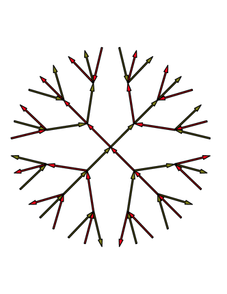
Figure 2 show the first two stages of the Cayley graph for and . The colored directed edges correspond to generators and will be described in more detail in the next subsection.


Labeling Edges and Vertices
We inductively describe how to label the vertices and how to label and orient the edges of the graph described above.
Remark 2.1.
Note that an edge oriented from to labeled with the generator is regarded the same as that edge oriented from to and labeled with the generator .
Begin by labeling the vertex at the origin corresponding to the identity as . Label the vertex at for as .
Label the edge from to , with the generator and orient it from to . Note that this is equivalent to labeling the edge from to with the generator and orienting it from to . For notation, we refer to this edge as or to emphasize the initial vertex and generator needed to get to the other vertex. To emphasize the initial and final vertices, we can use the notation .
Note that starting at any point on the circle of radius centered at the origin and traveling in the counterclockwise direction around this circle, one encounters the labeled edges in the cyclic order , or equivalently, by Remark 2.1, in the cyclic order:
.
Inductively assume the vertices at distance from the origin, , have been labeled as , where is a reduced word of length . Also assume that edges from vertices at distance from the origin to at distance from the origin have been labeled where .
Consider for some of reduced length n. Then for some reduced word of length and some . The edge joining to is labeled , or equivalently . Let .
Form a circle of radius about . Starting at the edge , proceed around the circle in the counterclockwise direction labeling the edges encountered as
all subscripts mod(2N).


Label the vertices at distance from the origin as follows. If is such a vertex, then there is an edge from a vertex at distance from the origin to . Label the vertex as .
Cayley Graph Automorphisms for
For each element of we define a graph automorphism of as follows. For a vertex of corresponding to the element of , is defined to be . The edge from to can be labeled when oriented from to . Define to be the linear homeomorphism from to .
Remark 2.2.
Note that these graph automorphisms define homeomorphisms from to itself. Note also that .
Extending Graph Automorphisms to Homeomorphisms of
The graph automorphisms , for , can be extended to homeomorphisms from to itself. Note that consists of a collections of unbounded regions with boundary in . Adding in the point at infinity, each region is a closed disc with boundary consisting of edges in together with this added point. The graph automorphism takes the boundary of one of these disc regions to the boundary of another, and can thus be extended to the entire region. There are many choices for these extension homeomorphisms. They coincide up to proper isotopy.
Piecing together these extensions, one gets an extension of to a self homeomorphism of , for . Define for to be . Since for as graph automorphisms, it follows that is an extension of for .
For a general , has a unique reduced representation where the are in . Define to be:
The homeomorphism can then be extended to a homeomorphism by crossing with the identity.
Remark 2.3.
Note that . This follows from the uniqueness of reduced representations of elements of . The definition of as the product of with the identity shows that it is also true that .
3. A Cantor Set with Embedding Homogeneity Group
A Collection of Balls and Tubes in Containing
In , choose a 3-ball around the origin so that the homeomorphic copies , together with are all pairwise disjoint. Let denote the 3-ball . The original ball can be chosen so that it is contained in a ball of radius about , and so that each is contained in a ball of radius about .
For a general , use the unique reduced representation of as where the are in . The ball is then defined to be to be:
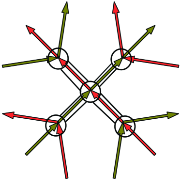
We similarly define a collection of tubes. For each , choose a thin tube joining to so that contains . Choose the tubes , so as to be pairwise disjoint. For each , let be . See Figure 4 for an illustration for .
Remark 3.1.
Note that the relationship then holds for all , .
Rigid Cantor Sets Using as a Guide.
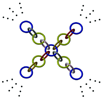
We will now define rigid Antoine Cantor sets associated with each vertex in , and a chain of three linked rigid Cantor sets for each edge in . See Figure 5 for an illustration of the outer tori in defining sequences for these rigid Cantor sets in the case of .
To begin, construct a rigid Antoine Cantor set so the outer torus, , of the construction is in . This corresponds to the central torus in Figure 5 in the case of . Let be the union of the second stage tori in the construction of . See Figure 1 for an illustration of the first and second stages of an Antoine construction.
For a general , use the unique reduced representation of as where the are in . Define a rigid Cantor set to be:
Remark 3.2.
Note that and any are equivalently embedded.
Similarly, let The four outer tori in Figure 5 correspond to , and in the case of .
We next construct rigid Cantor sets for each . Choose a series of three linked tori, and joining and contained in as in Figure 5. Label the torus linked to as , and use it as the outer torus for a rigid Antoine Cantor set . Label the torus linked to as , and use it as the outer torus for a rigid Antoine Cantor set . Label the remaining torus as and use it as the outer torus for a rigid Antoine Cantor set .
Remark 3.3.
Choose these rigid Cantor sets so that they are all inequivalently embedded, and so that they are all inequivalent to .
For , and , let , and . This completes the definition of the rigid Cantor sets along the edges . See Figure 5 for outer tori corresponding to these Cantor sets in the case .
For , let and for and .
For any rigid Antoine Cantor set in this construction, represents the outer torus in the Antoine Construction and represents the union of the second stage tori in the construction.
Remark 3.4.
Because are identified, it appears that there are two possible definitions for the on this edge: and . However,
Remark 3.5.
Note that none of the are equivalent to any , and that is equivalent to if and only if one of the following two conditions holds:
The union of the Cantor sets together with the union of the Cantor sets is not a Cantor set since it is not compact. To remedy this, we add the point at infinity, denoted by , to to get . We then define the Cantor set associated with to be:
4. Main Theorems
We now have . One can show that cannot be separated by any 2-sphere, by an argument similar to that referred to in Remark 1.9. Let be the 3-manifold . By Remark 1.7, is irreducible.
We will show that the embedding homogeneity group of is , and correspondingly, that the end homogeneity group of is .
We use the following three technical lemmas in the proof of Theorem 4.6 below. In reading the first lemma, think of and as two linked tori in a stage of an Antoine construction as in Figure 1. The second lemma shows that homeomorphisms of taking to itself necessarily fix the point . The third lemma shows that homeomorphisms of taking some to some , when restricted to , agree with some restricted to .
Lemma 4.1.
Let , and be rigid Antoine Cantor sets in . Let and be the first and second stages in the construction of . Assume that and are linked (and thus are disjoint). Let be a homeomorphism such that
-
**
.
Assume in addition that
-
a)
,
-
b)
, and
-
c)
.
If , then
-
I)
either the geometric index of in is 0, is also contained in , and the geometric index of in is also 0,
-
II)
or the geometric index of in is and .
Proof.
We have and we consider the geometric index of in .
Index 0: Assume that the geometric index is . Then is contained in a cell in , and so contracts in .
If does not intersect , then either , or misses . The last case cannot occur because of the linking of and . In the first case, and the geometric index of in is . So condition (I) holds. The second case cannot occur because and are disjoint.
If does intersect , then by (a) above. If the geometric index of in is , then cannot be contained in any component of by Theorem 1.2. Thus, by (a), contains any component of that it intersects. By (c), . So intersects and thus contains some component of . The geometric index of in must be by Theorem 1.2. Thus is contained in a cell in and contracts in .
Let be the components of , listed so that links . Since and are linked, the Antoine construction guarantees that any contraction of intersects . So intersects and thus contains and has geometric index 0 in . Continuing inductively, all of the are contained in and thus contains .
Since is disjoint from , this contradicts condition **.
Index greater than 1: If the geometric index of in is greater than , then by Theorem 1.2, cannot be contained in any component of . So contains each component of that it intersects. Let be the components of , listed so that links . By condition **, intersects and thus contains some component of , say . The geometric index of in is 0 by Theorem 1.2.
By an argument similar to that in the Index 0 case above, contains each , and each is of index 0 in . By Theorem 1.3, the geometric index of in is even. Since the geometric index of in is two [1], the geometric index of in cannot be and so is at least two. Theorem 1.2 now implies that the geometric index of in is at least 4, which is a contradiction. So the the geometric index of in cannot be greater than .
Index equal to 1: If the geometric index of in is , then by Theorem 1.2, cannot be contained in any component of . An argument similar to that in the previous two cases shows that contains each component of . Thus . So condition (II) holds. ∎
Lemma 4.2.
Let be a homeomorphism that extends to a homeomorphism of . Then .
Proof.
The local genus of any point in other than is less than or equal to one because these points are defined by nested sequences of tori which are of genus one. If we can show the local genus of is at least 2, then the results mentioned in Remark 1.5 show that .
Remark 4.3.
The local genus of in cannot be because otherwise, there would be arbitrarily small 3-balls containing with boundary missing . These boundary 2-spheres in the complement of would separate linked stages of some Antoine construction. This cannot happen.

To see that the local genus of in is at least 2, consider 2 subsets of that meet in . These subsets are obtained by dividing into two subsets that meet in .
For a nonidentity , with unique reduced representation as where the are in , let .
Figure 6 illustrates the start of the described construction in the case . The Cantor set arises from tori in the upper half of the figure, and the Cantor set set arises from tori in the lower half of the figure.
Note that and intersect in . The local genus of in each of these Cantor sets is at least 1 by reasoning similar to that in Remark 4.3.
The satisfy the conditions of Theorem 1.6. It follows that the genus of in is 2.
Note: In fact, the local genus of in is . ∎
Lemma 4.4.
If is a self homeomorphism of and for some with then . In particular, if for some , then .
Proof.
. So both and take onto . Thus takes onto . The rigidity of implies that . ∎
Theorem 4.5 (Main Theorem).
is an irreducible 3-manifold with end homogeneity group .
This follows immediately from the next theorem.
Theorem 4.6.
is unsplittable and the embedding homogeneity group of is .
Proof.
The unsplittability was addressed above. Let be the embedding homogeneity group of . Note that the homeomorphisms , extend to homeomorphisms , by fixing the point at infinity.
For each , let . Then each takes onto . This follows directly from the definition of and . The elements form a subgroup of since by Remark 2.2.
Let be any self homeomorphism of that extends to a homeomorphism of . We will show that for some .
Step 1: We first show that for some . If this is true, then the definition of as and Lemma 4.4 shows that Let:
does not contain by Lemma 4.2. So there is a positive integer such that . Similarly, there is a positive integer such that .
Using techniques similar to those in [18], or [11], choose a homeomorphism of to itself, fixed on , so that
| (1) |
Let . Let be a point of and let where (or ) for some and where (or ). We will show that in fact, for some , and that the second case above cannot occur. Observe that either or by Equation 1 above.
Step 1a: Assume that . Lemma 4.1 now applies with . If has geometric index in , choose a linked chain of tori in the construction of joining to a where . By repeated applications of Lemma 4.1 it follows that which is a contradiction. So has geometric index greater than or equal to in . By Lemma 4.1, this geometric index is 1 and .
Since , we have . Since in not equivalent to any by Remarks 3.3 and 3.5 we get for some . It follows from Lemma 4.4 that .
Step 1b: Assume that . Then . The argument from Case I can now be repeated replacing by and interchanging and . It follows that and so for some as claimed. Again it follows from Lemma 4.4 that .
Step 2: By an argument similar to that in Step 1, for each for some . Also for each , and ,
for some .
Working inductively outward from , and using the fact that if and are linked tori, then and are linked, one sees that each and each .
By Lemma 4.4 it follows that each , and that each It now follows that for the from Steps 1 and 2. This shows that is in fact, the group and that is isomorphic to . ∎
The method used in the construction of can be used for any Cayley graph of a finitely generated group for which the graph automorphisms have certain extension properties. This observation is given in the next theorem.
Theorem 4.7.
Suppose is a finitely presented group with a Cayley Graph in . Suppose the graph automorphisms for can be extended to homeomorphisms of . Suppose also that for every pair of group elements , . Then there is an open irreducible 3-manifold with embedding homogeneity group isomorphic to .
Proof.
The construction of a collection of Cantor sets modeled on the graph, and the proof analogous to the proof of Theorem 4.6 go through in this case. ∎
Questions
In [10], the authors showed that for every finitely generated abelian group , there is an irreducible open 3-manifold with end homogeneity group isomorphic to . In this paper, we show that for any finitely generated free group , there is an irreducible open 3-manifold with end homogeneity group .
Question (1).
Which non-abelian finitely generated groups can arise as end homogeneity groups of (irreducible) open 3-manifolds?
In light of Theorem 4.7, this leads to the following question.
Question (2).
Which non-abelian finitely generated groups have Cayley graphs embeddable in with the properties listed in Theorem 4.7?
A related question is the following.
Question (3).
If not all finitely generated non-abelian groups have Cayley graphs with the properties listed in Theorem 4.7, is there a way to characterize which ones do have this property?
Appendix
This section lists some of the important notation used in the paper.
-
•
is the free group on N generators.
-
•
, is the full set of generators for .
-
•
for and for .
-
•
is the Cayley graph constructed in for .
-
•
are vertices of associated with group elements.
-
•
is the oriented edge labeled from to .
This edge is the regarded the same as . -
•
is the automorphism of given by ,
. -
•
is the extension of to a homeomorphism of .
-
•
is a 3-ball about the vertex .
-
•
is a tube joining to .
-
•
is a rigid Cantor set in .
-
•
, form a linked chain of rigid Cantor sets joining to . .
-
•
. .
Acknowledgements
The authors would like to thank the referee for many helpful suggestions and comments. These suggestions helped to clarify the arguments in the paper. Both authors were supported in part by the Slovenian Research Agency grant BI-US/19-21-024. The second author was supported in part by the Slovenian Research Agency grants P1-0292, N1-0114, N1-0083, N1-0064, and J1-8131.
References
- [1] Kathryn B. Andrist, Dennis J. Garity, Dušan D. Repovš, and David G. Wright. New techniques for computing geometric index. Mediterr. J. Math., 14(6):Art. 237, 15, 2017.
- [2] M. L. Antoine. Sur la possibilite d’etendre l’homeomorphie de deux figures a leur voisinages. C.R. Acad. Sci. Paris, 171:661–663, 1920.
- [3] Robert J. Daverman. Embedding phenomena based upon decomposition theory: wild Cantor sets satisfying strong homogeneity properties. Proc. Amer. Math. Soc., 75(1):177–182, 1979.
- [4] R. F. Dickman, Jr. Some characterizations of the Freudenthal compactification of a semicompact space. Proc. Amer. Math. Soc., 19:631–633, 1968.
- [5] Jan J. Dijkstra. Homogeneity properties with isometries and Lipschitz functions. Rocky Mountain J. Math., 40(5):1505–1525, 2010.
- [6] Alastair Fletcher and Jang-Mei Wu. Julia sets and wild Cantor sets. Geom. Dedicata, 174:169–176, 2015.
- [7] Hans Freudenthal. Neuaufbau der Endentheorie. Ann. of Math. (2), 43:261–279, 1942.
- [8] Dennis J. Garity, Dušan Repovš, David Wright, and Matjaž Željko. Distinguishing Bing-Whitehead Cantor sets. Trans. Amer. Math. Soc., 363(2):1007–1022, 2011.
- [9] Dennis J. Garity and Dušan Repovš. Inequivalent Cantor sets in whose complements have the same fundamental group. Proc. Amer. Math. Soc., 141(8):2901–2911, 2013.
- [10] Dennis J. Garity and Dušan Repovš. Homogeneity groups of ends of open 3-manifolds. Pacific J. Math., 269(1):99–112, 2014.
- [11] Dennis J. Garity, Dušan Repovš, and David Wright. Simply connected open 3-manifolds with rigid genus one ends. Rev. Mat. Complut., 27(1):291–304, 2014.
- [12] Dennis J. Garity, Dušan Repovš, and Matjaž Željko. Uncountably many Inequivalent Lipschitz Homogeneous Cantor Sets in . Pacific J. Math., 222(2):287–299, 2005.
- [13] Dennis J. Garity, Dušan Repovš, and Matjaž Željko. Rigid Cantor sets in with Simply Connected Complement. Proc. Amer. Math. Soc., 134(8):2447–2456, 2006.
- [14] Dennis J. Garity, Dušan D. Repovš, and David G. Wright. Contractible 3-manifolds and the double 3-space property. Trans. Amer. Math. Soc., 370(3):2039–2055, 2018.
- [15] Paul Gartside and Merve Kovan-Bakan. On the space of Cantor subsets of . Topology Appl., 160(10):1088–1098, 2013.
- [16] José María Montesinos-Amilibia. On some groups related with Fox-Artin wild arcs. J. Knot Theory Ramifications, 25(3):1640007, 27, 2016.
- [17] H. Schubert. Knoten und vollringe. Acta. Math., 90:131–186, 1953.
- [18] R. B. Sher. Concerning wild Cantor sets in . Proc. Amer. Math. Soc., 19:1195–1200, 1968.
- [19] A. C. Shilepsky. A rigid Cantor set in . Bull. Acad. Polon. Sci. Sér. Sci. Math., 22:223–224, 1974.
- [20] Laurence Carl Siebenmann. The Obstruction to Finding a Boundary for an Open Manifold of Dimension Greater than Five. ProQuest LLC, Ann Arbor, MI, 1965. Thesis (Ph.D.)–Princeton University.
- [21] Juan Souto and Matthew Stover. A Cantor set with hyperbolic complement. Conform. Geom. Dyn., 17:58–67, 2013.
- [22] Jan van Mill. On countable dense and strong -homogeneity. Fund. Math., 214(3):215–239, 2011.
- [23] David G. Wright. Rigid sets in . Pacific J. Math., 121(1):245–256, 1986.
- [24] Matjaž Željko. Genus of a Cantor set. Rocky Mountain J. Math., 35(1):349–366, 2005.