FrAug: Frequency Domain Augmentation for Time Series Forecasting
Abstract
Data augmentation (DA) has become a de facto solution to expand training data size for deep learning. With the proliferation of deep models for time series analysis, various time series DA techniques are proposed in the literature, e.g., cropping-, warping-, flipping-, and mixup-based methods. However, these augmentation methods mainly apply to time series classification and anomaly detection tasks. In time series forecasting (TSF), we need to model the fine-grained temporal relationship within time series segments to generate accurate forecasting results given data in a look-back window. Existing DA solutions in the time domain would break such a relationship, leading to poor forecasting accuracy. To tackle this problem, this paper proposes simple yet effective frequency domain augmentation techniques that ensure the semantic consistency of augmented data-label pairs in forecasting, named FrAug. We conduct extensive experiments on eight widely-used benchmarks with several state-of-the-art TSF deep models. Our results show that FrAug can boost the forecasting accuracy of TSF models in most cases. Moreover, we show that FrAug enables models trained with 1% of the original training data to achieve similar performance to the ones trained on full training data, which is particularly attractive for cold-start forecasting. Finally, we show that applying test-time training with FrAug greatly improves forecasting accuracy for time series with significant distribution shifts, which often occurs in real-life TSF applications. Our code is available at https://anonymous.4open.science/r/Fraug-more-results-1785.
1 Introduction
Deep learning is notoriously data-hungry. Without abundant training data, deep models tend to suffer from poor convergence or overfitting problems. Since collecting and labeling real-world data can be costly and time-consuming, data augmentation (DA) has become a de facto solution to expand the training dataset size for performance improvement [?].
With the proliferation of deep models for time series analysis, various time series DA techniques are proposed in the literature. As shown in [?], most of them focus on the classification and the anomaly detection (AD) tasks, partly because the time series forecasting (TSF) task comes with natural labels without extra labeling efforts. However, the TSF task may also suffer from severe data scarcity problems. For example, one important use case, cold-start forecasting, performs time series forecasting (TSF) with little or no historical data, e.g., sales prediction for new products. More importantly, even for time series with sufficient historical data, there might be significant distribution shifts in the forecasting horizon, rendering historical data less useful [?]. Under such circumstances, we need to retrain the forecasting model to fit the new data distribution. Consequently, effective DA techniques are essential for the TSF task.
When using data augmentation for supervised learning, we create artificial data-label pairs from existing labeled data. It is critical to ensure the semantic consistency of such modified data-label pairs. Otherwise, augment ambiguity is introduced, thereby deteriorating the performance of the model instead of improving it, as examined in several previous works in the computer vision (CV) field [?; ?]. In fact, DA for image data is less ambiguous when compared to that for time series data, because image data are relatively easy to interpret, enabling us to create semantics-preserving augmentations (e.g., rotation and cropping/masking less relevant regions).
In contrast, time series data are comprised of events generated from complicated dynamic systems. We are interested in the temporal relationship among continuous data points in the series. As any perturbations would change such a relationship, care must be taken to ensure that the semantics of the data-label pair is preserved, i.e., they are likely to occur according to the behavior of the underlying system. For time series classification, we could perform window cropping [?; ?], window warping [?], and noise injection [?] on time series without changing the classification labels as long as such manipulations do not yield class changes. Similarly, label expansion [?] that manipulates the “blurry” start and end points of sequence anomalies brings performance improvements for the anomaly detection task.
However, time series forecasting is a regression task. It requires modeling the fine-grained temporal relationship within a timing window divided into two parts: the data points in the look-back window and those in the forecasting horizon, serving as the data and the label when training TSF models, respectively. Aggressive augmentation methods such as cropping or warping would cause missing values or periodicity changes in the series and hence do not apply to TSF models. In other words, the augmented data-label pairs for TSF should be much more stringent than those for other time series analysis tasks, which have not been thoroughly investigated in the literature.
In this paper, we argue that well-designed data augmentations in the frequency domain can preserve the fine-grained temporal relationship within a timing window. For a dynamic system that generates time series data, its forecastable behavior is usually driven by some periodical events222The measurements contributed by random events are not predictable.. By identifying and manipulating such events in the frequency domain, the generated data-label pairs would remain faithful to the underlying dynamic system. This motivates us to propose two simple yet effective frequency domain augmentation methods for TSF, named FrAug. Specifically, FrAug performs frequency masking and frequency mixing, which randomly eliminate some frequency components of a timing window or mix up the same frequency components of different timing windows. Experimental results on eight widely-used TSF benchmark datasets show that FrAug improves the forecasting accuracy of various deep models, especially when the size of the training dataset is small, e.g., for cold-start forecasting or forecasting under distribution shifts.
Specifically, the main contributions of this work include:
-
•
To the best of our knowledge, this is the first work that systematically investigates data augmentation techniques for the TSF task.
-
•
We propose a novel frequency domain augmentation technique named FrAug, including two simple yet effective methods (i.e., frequency masking and frequency mixing) that preserve the semantic consistency of augmented data-label pairs in forecasting. In our experiments, we show that FrAug alleviates overfitting problems of state-of-the-art (SOTA) TSF models, thereby improving their forecasting performance.
-
•
FrAug enables models trained with 1% of the original training data to achieve similar performance to the ones trained on full training data in some datasets, which is particularly attractive for cold-start forecasting problems.
-
•
We further design a test-time training policy and apply FrAug to expand the training dataset size. We experimentally show that such a strategy greatly mitigates the distribution shift problem, thereby boosting forecasting accuracy considerably. In particular, for the ILI dataset with severe distribution shifts, we can achieve up to 30% performance improvements.
2 Related Work and Motivation
Data augmentation methods are task-dependent. In this section, we first analyze the challenges in time-series forecasting in Sec. 2.1. Next, in Sec. 2.2, we survey existing DA techniques for time series analysis and discuss why they do not apply to the forecasting task. Finally, we discuss the motivations behind the proposed FrAug solution in Sec. 2.3.
2.1 Challenges in Time Series Forecasting
Given the data points in a look-back window of multivariate time series, where is the look-back window size, C is the number of variates, and is the value of the variate at the time step. The TSF task is to predict the horizon , the values of all variates at future T time steps. When the forecasting horizon is large, it is referred to as a long-term forecasting problem, which has attracted lots of attention in recent research [?; ?].
Deep learning models have dominated the TSF field in recent years, achieving unparalleled forecasting accuracy for many problems, thanks to their ability to capture complicated temporal relationships of the time series by fitting on a large amount of data. However, in many real applications, time series forecasting remains challenging for two main reasons.
First, the training data can be scarce. Unlike computer vision or natural language processing tasks, time series data are relatively difficult to scale. Generally speaking, for a specific application, we can only collect real data when the application is up and running. Data from other sources are often not useful (even if they are the same kinds of data), as the underlining dynamic systems that generate the time series data could be vastly different. In particular, lack of data is a serious concern in cold-start forecasting and long-term forecasting. In cold-start forecasting, e.g., sales prediction for new products, we have no or very little historical data for model training. In long-term forecasting tasks, the look-back window and forecasting horizon are large, requiring more training data for effective learning. Over-fitting caused by data scarcity is observed in many state-of-the-art models training on several benchmark time-series datasets.
Second, some time-series data exhibits strong distribution shifts over time. For example, promotions of products can increase the sales of a product and new economic policies would significantly affect financial data. When such a distribution shift happens, the model trained on previous historical data cannot work well. To adapt to a new distribution, a common choice is re-training the model on data with the new distribution. However, data under the new distribution is scarce and takes time to collect.
| Method | Origin | Noise | Noise* | Mask-Rand. | Mask-Seg. | Flipping | Warping |
|---|---|---|---|---|---|---|---|
| DLinear | 0.373 | 0.444 | 0.371 | 0.803 | 0.448 | 0.544 | 0.401 |
| FEDformer | 0.374 | 0.380 | 0.397 | 0.448 | 0.433 | 0.420 | 0.385 |
| Autoformer | 0.449 | 0.460 | 0.476 | 0.608 | 0.568 | 0.446 | 0.465 |
| Informer | 0.931 | 0.936 | 1.112 | 0.846 | 1.013 | 0.955 | 1.265 |
2.2 Data Augmentation Methods for Time Series Analysis
Various time series DA techniques are proposed in the literature. For the time series classification task, many works regard the series as a waveform image and borrow augmentation methods from the CV field, e.g., window cropping [?], window flipping [?], and Gaussian noise injection [?]. There are also DA methods that take advantage of specific time series properties, e.g., window warping [?], surrogate series [?; ?], and time-frequency feature augmentation [?; ?; ?; ?]. For the time series AD task, window cropping and window flipping are also often used. In addition, label expansion and amplitude/phase perturbations are introduced in [?].
With the above, one may consider directly applying these DA methods to the forecasting task to expand training data. We perform such experiments with several popular TSF models, and the results are shown in Table 1. As can be observed, these DA techniques tend to generate reduced forecasting accuracy. The reason is rather simple: most of these DA methods introduce perturbation in the time domain (e.g., noise or zero masking), and the augmented data-label pairs do not preserve the semantics consistency required by the TSF task.
There are also a few DA techniques for the forecasting task presented in the literature. [?] proposes DATSING, a transfer learning-based framework that leverages cross-domain time series latent representations to augment target domain forecasting. [?] introduces two DA methods for forecasting: (i). Average selected with distance (ASD), which generates augmented time series using the weighted sum of multiple time series [?], and the weights are determined by the dynamic time warping (DTW) distance; (ii). Moving block bootstrapping (MBB) generates augmented data by manipulating the residual part of the time series after STL decomposition [?] and recombining it with the other series. It is worth noting that, in these works, data augmentation is not the focus of their proposed framework, and the design choices for their augmentation strategies are not thoroughly discussed.
2.3 Why Frequency Domain Augmentation?
The forecastable behavior of time series data is usually driven by some periodical events. For example, the hourly sampled power consumption of a house is closely related to the periodical behavior of the householder. His/her daily routine (e.g., out for work during the day and activities at night) would introduce a daily periodicity, his/her routines between weekdays and weekends would introduce a weekly periodicity, while the yearly atmosphere temperature change would introduce an annual periodicity. Such periodical events can be easily decoupled in the frequency domain and manipulated independently.
Motivated by the above, we propose to perform frequency domain augmentation for the TSF task. By identifying and manipulating events in the frequency domain for data points in both the look-back window and forecasting horizon, the resulting augmented data-label pair would largely conform to the behavior of the underlying system.
3 Methods
In this section, we detail the proposed frequency domain data augmentation methods for time series forecasting.
3.1 The Pipeline of FrAug
To ensure the semantic consistency of augmented data-label pairs in forecasting, we add frequency domain perturbations on the concatenated time series of the look-back window and target horizon, with the help of the Fast Fourier transform (FFT) as introduced in Appendix. We only apply FrAug during the training stage and use original test samples for testing.
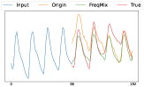
As shown in Figure 1, in the training stage, given a training sample (data points in the look-back window and the forecasting horizon), FrAug (i) concatenates the two parts, (ii) performs frequency domain augmentations, and (iii) splits the concatenated sequence back into lookback window and target horizon in the time domain. The augmentation result of an example time series training sample is shown in Figure 2.


3.2 Frequency Masking and Frequency Mixing
We propose two simple yet effective augmentation methods under FrAug framework, namely Frequency Masking and Frequency Mixing. Specifically, frequency masking randomly masks some frequency components, while frequency mixing exchanges some frequency components of two training samples in the dataset.
Frequency masking: The pipeline of frequency masking is shown in Figure 3(a). For a training sample comprised of data points in the look-back window and the forecasting horizon , we first concatenate them in the time domain as and apply real FFT to calculate the frequency domain representation , which is a tensor composed of the complex number. Next, we randomly mask a portion of this complex tensor as zero and get . Finally, we apply inverse real FFT to project the augmented frequency domain representation back to the time domain . The detailed procedure is shown in Algorithm 1.
Frequency Masking corresponds to removing some events in the underlying system. For example, considering the household power consumption time series, removing the weekly frequency components would create an augmented time series that belongs to a house owner that has similar activities on the weekdays and weekends.
Frequency mixing: The pipeline of frequency mixing is shown in Figure 3, wherein we randomly replace the frequency components in one training sample with the same frequency components of another training sample in the dataset. The details of this procedure are presented in Algorithm 2.
Similarly, frequency mixing can be viewed as exchanging events between two samples. For the earlier example on household power consumption, the augmented time series could be one owner’s weekly routine replaced by another’s, and hence the augmented data-label pair largely preserves semantical consistency for forecasting.
Note that, frequency masking and frequency mixing only utilize information from the original dataset, thereby avoiding the introduction of unexpected noises compared to those dataset expansion techniques based on synthetic generation [?; ?]. Moreover, as the number of combinations of training samples and their frequencies components in a dataset is extremely large, FrAug can generate nearly infinite reasonable samples.
4 Experiments
In this section, we apply FrAug to three TSF application scenarios: long-term forecasting, cold-start forecasting, and test-time training. Due to space limitations, the experimental results for other applications (e.g., short-term forecasting) and ablation studies are presented in the Appendix.
4.1 Experimental Setup
| Dataset | Exchange-Rate | Traffic | Electricity | Weather | ETTh1ETTh2 | ETTm1 ETTm2 | ILI |
|---|---|---|---|---|---|---|---|
| Variates | 8 | 862 | 321 | 21 | 7 | 7 | 7 |
| Frequency | 1day | 1hour | 1hour | 10min | 1hour | 5min | 1week |
| Total Timesteps | 7,588 | 17,544 | 26,304 | 52,696 | 17,420 | 69,680 | 966 |
| Model | Method | ETTh1 | ETTh2 | ETTm1 | ETTm2 | ||||||||||||
|---|---|---|---|---|---|---|---|---|---|---|---|---|---|---|---|---|---|
| 96 | 192 | 336 | 720 | 96 | 192 | 336 | 720 | 96 | 192 | 336 | 720 | 96 | 192 | 336 | 720 | ||
| DLinear | Original | 0.374 | 0.405 | 0.439 | 0.514 | 0.295 | 0.378 | 0.421 | 0.696 | 0.300 | 0.335 | 0.368 | 0.425 | 0.171 | 0.235 | 0.305 | 0.412 |
| FreqMask | 0.372 | 0.407 | 0.453 | 0.473 | 0.282 | 0.344 | 0.443 | 0.592 | 0.297 | 0.332 | 0.368 | 0.428 | 0.166 | 0.228 | 0.281 | 0.399 | |
| FreqMix | 0.372 | 0.409 | 0.438 | 0.482 | 0.284 | 0.346 | 0.449 | 0.636 | 0.297 | 0.332 | 0.372 | 0.428 | 0.168 | 0.229 | 0.286 | 0.398 | |
| ASD | 0.387 | 0.554 | 0.445 | 0.467 | 0.302 | 0.363 | 0.411 | 0.677 | 0.311 | 0.343 | 0.377 | 0.430 | 0.188 | 0.237 | 0.297 | 0.400 | |
| MBB | 0.389 | 0.423 | 0.508 | 0.521 | 0.313 | 0.391 | 0.433 | 0.651 | 0.307 | 0.339 | 0.373 | 0.428 | 0.177 | 0.242 | 0.323 | 0.430 | |
| Fedformer | Original | 0.374 | 0.425 | 0.456 | 0.485 | 0.339 | 0.430 | 0.519 | 0.474 | 0.364 | 0.406 | 0.446 | 0.533 | 0.189 | 0.253 | 0.327 | 0.438 |
| FreqMask | 0.374 | 0.421 | 0.457 | 0.474 | 0.323 | 0.414 | 0.484 | 0.446 | 0.360 | 0.404 | 0.453 | 0.527 | 0.184 | 0.249 | 0.322 | 0.430 | |
| FreqMix | 0.371 | 0.418 | 0.466 | 0.497 | 0.327 | 0.421 | 0.507 | 0.466 | 0.361 | 0.404 | 0.447 | 0.515 | 0.184 | 0.252 | 0.326 | 0.432 | |
| ASD | 0.429 | 0.455 | 0.561 | 0.582 | 0.339 | 0.429 | 0.501 | 0.454 | 0.390 | 0.430 | 0.514 | 0.585 | 0.200 | 0.264 | 0.345 | 0.460 | |
| MBB | 0.412 | 0.460 | 0.501 | 0.514 | 0.356 | 0.455 | 0.526 | 0.484 | 0.385 | 0.427 | 0.477 | 0.548 | 0.211 | 0.270 | 0.340 | 0.439 | |
| Autoformer | Original | 0.449 | 0.463 | 0.495 | 0.535 | 0.432 | 0.430 | 0.482 | 0.471 | 0.552 | 0.559 | 0.605 | 0.755 | 0.288 | 0.274 | 0.335 | 0.437 |
| FreqMask | 0.434 | 0.426 | 0.495 | 0.597 | 0.347 | 0.425 | 0.474 | 0.465 | 0.419 | 0.513 | 0.481 | 0.595 | 0.232 | 0.264 | 0.325 | 0.421 | |
| FreqMix | 0.401 | 0.484 | 0.471 | 0.517 | 0.351 | 0.423 | 0.494 | 0.538 | 0.410 | 0.542 | 0.497 | 0.769 | 0.212 | 0.265 | 0.325 | 0.433 | |
| ASD | 0.486 | 0.497 | 0.530 | 0.499 | 0.362 | 0.442 | 0.477 | 0.523 | 0.561 | 0.532 | 0.518 | 0.616 | 0.233 | 0.276 | 0.331 | 0.444 | |
| MBB | 0.479 | 0.526 | 0.592 | 0.602 | 0.363 | 0.431 | 0.472 | 0.547 | 0.535 | 0.652 | 0.704 | 0.522 | 0.239 | 0.283 | 0.334 | 0.454 | |
| Informer | Original | 0.931 | 1.010 | 1.036 | 1.159 | 2.843 | 6.236 | 5.418 | 3.962 | 0.626 | 0.730 | 1.037 | 0.972 | 0.389 | 0.813 | 1.429 | 3.863 |
| FreqMask | 0.637 | 0.788 | 0.873 | 1.042 | 2.555 | 3.983 | 3.752 | 2.561 | 0.425 | 0.538 | 0.783 | 0.846 | 0.368 | 0.463 | 0.984 | 3.932 | |
| FreqMix | 0.675 | 1.021 | 1.044 | 1.100 | 2.774 | 5.940 | 4.718 | 4.088 | 0.593 | 0.702 | 0.867 | 0.930 | 0.341 | 0.557 | 1.322 | 2.939 | |
| ASD | 0.853 | 1.020 | 1.124 | 1.226 | 2.280 | 5.830 | 4.345 | 3.886 | 0.726 | 0.775 | 0.921 | 0.968 | 0.405 | 0.874 | 1.317 | 2.585 | |
| MBB | 0.958 | 1.031 | 1.049 | 1.227 | 3.112 | 6.398 | 5.668 | 4.007 | 0.630 | 0.731 | 0.988 | 0.961 | 0.399 | 0.783 | 1.476 | 4.012 | |
| Model | Method | Exchange Rate | Electricity | Traffic | Weather | ||||||||||||
|---|---|---|---|---|---|---|---|---|---|---|---|---|---|---|---|---|---|
| 96 | 192 | 336 | 720 | 96 | 192 | 336 | 720 | 96 | 192 | 336 | 720 | 96 | 192 | 336 | 720 | ||
| DLinear | Original | 0.079 | 0.205 | 0.309 | 1.029 | 0.140 | 0.154 | 0.169 | 0.204 | 0.410 | 0.423 | 0.436 | 0.466 | 0.175 | 0.217 | 0.265 | 0.324 |
| FreqMask | 0.101 | 0.182 | 0.263 | 0.842 | 0.140 | 0.154 | 0.169 | 0.204 | 0.411 | 0.423 | 0.435 | 0.466 | 0.174 | 0.217 | 0.265 | 0.324 | |
| FreqMix | 0.099 | 0.187 | 0.274 | 0.883 | 0.140 | 0.154 | 0.169 | 0.204 | 0.412 | 0.423 | 0.435 | 0.467 | 0.174 | 0.216 | 0.264 | 0.324 | |
| ASD | 0.102 | 0.273 | 0.294 | 0.787 | 0.163 | 0.175 | 0.189 | 0.222 | 0.437 | 0.450 | 0.463 | 0.493 | 0.195 | 0.230 | 0.275 | 0.329 | |
| MBB | 0.080 | 0.204 | 0.308 | 1.021 | 0.145 | 0.157 | 0.172 | 0.206 | 0.420 | 0.430 | 0.441 | 0.467 | 0.176 | 0.217 | 0.262 | 0.324 | |
| Fedformer | Original | 0.135 | 0.271 | 0.454 | 1.140 | 0.188 | 0.196 | 0.212 | 0.250 | 0.574 | 0.611 | 0.623 | 0.631 | 0.250 | 0.266 | 0.368 | 0.397 |
| FreqMask | 0.129 | 0.238 | 0.469 | 1.149 | 0.176 | 0.196 | 0.204 | 0.220 | 0.572 | 0.586 | 0.612 | 0.631 | 0.231 | 0.240 | 0.308 | 0.373 | |
| FreqMix | 0.133 | 0.241 | 0.470 | 1.147 | 0.176 | 0.187 | 0.204 | 0.226 | 0.565 | 0.591 | 0.604 | 0.629 | 0.200 | 0.245 | 0.317 | 0.377 | |
| ASD | 0.149 | 0.265 | 0.441 | 1.128 | 0.192 | 0.205 | 0.214 | 0.243 | 0.573 | 0.601 | 0.608 | 0.613 | 0.700 | 0.513 | 0.623 | 0.649 | |
| MBB | 0.145 | 0.257 | 0.456 | 1.142 | 0.202 | 0.223 | 0.240 | 0.297 | 0.601 | 0.613 | 0.630 | 0.647 | 0.309 | 0.280 | 0.352 | 0.392 | |
| Autoformer | Original | 0.145 | 0.385 | 0.453 | 1.087 | 0.203 | 0.231 | 0.247 | 0.276 | 0.624 | 0.619 | 0.604 | 0.703 | 0.271 | 0.315 | 0.345 | 0.452 |
| FreqMask | 0.139 | 0.414 | 0.838 | 0.806 | 0.170 | 0.209 | 0.212 | 0.237 | 0.594 | 0.588 | 0.608 | 0.654 | 0.217 | 0.280 | 0.323 | 0.388 | |
| FreqMix | 0.155 | 0.668 | 0.615 | 2.093 | 0.163 | 0.189 | 0.204 | 0.243 | 0.559 | 0.618 | 0.583 | 0.649 | 0.252 | 0.302 | 0.334 | 0.388 | |
| ASD | 0.147 | 0.312 | 1.344 | 1.152 | 0.248 | 0.223 | 0.268 | 0.254 | 0.608 | 0.616 | 0.603 | 0.694 | 1.015 | 0.574 | 0.584 | 0.874 | |
| MBB | 0.152 | 0.273 | 0.472 | 1.641 | 0.231 | 0.317 | 0.269 | 0.272 | 0.628 | 0.650 | 0.658 | 0.664 | 0.237 | 0.349 | 0.376 | 0.451 | |
| Informer | Original | 0.879 | 1.147 | 1.562 | 2.919 | 0.305 | 0.349 | 0.349 | 0.391 | 0.736 | 0.770 | 0.861 | 0.995 | 0.452 | 0.466 | 0.499 | 1.260 |
| FreqMask | 0.534 | 1.023 | 1.074 | 1.102 | 0.262 | 0.282 | 0.287 | 0.304 | 0.674 | 0.683 | 0.715 | 0.799 | 0.199 | 0.298 | 0.356 | 0.529 | |
| FreqMix | 0.962 | 1.156 | 1.514 | 2.689 | 0.266 | 0.276 | 0.287 | 0.306 | 0.674 | 0.677 | 0.726 | 0.807 | 0.216 | 0.402 | 0.459 | 0.666 | |
| ASD | 0.994 | 1.132 | 1.669 | 1.924 | 0.317 | 0.331 | 0.334 | 0.348 | 0.812 | 0.747 | 0.805 | 0.900 | 0.342 | 0.452 | 0.529 | 0.644 | |
| MBB | 0.859 | 1.136 | 1.549 | 2.874 | 0.354 | 0.389 | 0.397 | 0.451 | 0.752 | 0.768 | 0.892 | 1.057 | 0.544 | 0.425 | 0.601 | 1.221 | |
Dataset. All datasets used in our experiments are widely-used and publicly available real-world datasets, including Exchange-Rate [?], Traffic, Electricity, Weather, ILI, ETT [?]. We summarize the characteristics of these datasets in Table 2.
Baselines. We compare FrAug, including Frequency Masking (FreqMask) and Frequency Mixing (FreqMix), with existing time-series augmentation techniques for forecasting, including ASD [?; ?] and MBB [?; ?].
Deep Models. In the main paper, we include four state-of-the-art deep learning models for long-term forecasting, including Informer [?], Autoformer [?], FEDformer [?] and DLinear [?]. In the Appendix, we also provide experiments on LightTs [?], Film [?], and SCINet [?]. The effectiveness of augmentations methods is evaluated by comparing the performance of the same model trained with different augmentations.
Evaluation metrics. Following previous works [?; ?; ?; ?; ?; ?; ?], we use Mean Squared Error (MSE) as the core metrics to compare forecasting performance.
Implementation. FreqMask and FreqMix only have one hyper-parameter, which is the mask rate/mix rate, respectively. In our experiments, we only consider 0.1, 0.2,0.3,0.4,0.5. We use cross-validation to select this hyper-parameter. More details are presented in the Appendix.
4.2 Long-term Forecasting
Table 3 and Table 4 show the results of long-term forecasting. We use different augmentation methods to double the size of the training dataset. As can be observed, FreqMask and FreqMix improve the performance of the original model in most cases. However, the performances of ASD and MBB are often inferior to the original model.
Notably, FreqMask improves DLinear’s performance by 16% in ETTh2 when the predicted length is 192, and it improves FEDformer’s performance by 28% and Informer’s performance by 56% for the Weather dataset when the predicted length is 96. Similarly, FreqMix improves the performance of Autoformer by 27% for ETTm2 with a predicted length of 96 and the performance of Informer by 35% for ETT2 with a predicted length of 720. These results indicate that FrAug is an effective DA solution for long-term forecasting, significantly boosting SOTA performance in many cases.


We attribute the performance improvements brought by FrAug to its ability to alleviate the over-fitting issues. Generally speaking, a large gap between the training loss and the test loss, the so-called generalization gap, is an indicator of over-fitting. Figure 4 demonstrates training loss and test error curves from deep models Autoformer and Informer. Without FrAug, the training loss of Autoformer and Informer decease with more training epochs, but the test errors increase. In contrast, when FrAug is applied to include more training samples, the test loss can decrease steadily until it is stable. This result clearly shows the benefits of FrAug.


In Figure 5, we visualize some prediction results with/without FrAug. Without FrAug, the model can hardly capture the scale of data, and the predictions show little correlation to the look-back window, i.e, there is a large gap between the last value of the look-back window and the first value of the predicted horizon. This indicates that the models are over-fitting. In contrast, with FrAug, the prediction is much more reasonable.
| Model | Method | ETTh2 | Exchange Rate | Electricity | Traffic | ||||||||||||
|---|---|---|---|---|---|---|---|---|---|---|---|---|---|---|---|---|---|
| 96 | 192 | 336 | 720 | 96 | 192 | 336 | 720 | 96 | 192 | 336 | 720 | 96 | 192 | 336 | 720 | ||
| DLinear | Full Data | 0.295 | 0.378 | 0.421 | 0.696 | 0.079 | 0.205 | 0.309 | 1.029 | 0.140 | 0.154 | 0.169 | 0.204 | 0.410 | 0.423 | 0.436 | 0.466 |
| 1% Data | 0.572 | 0.704 | 0.628 | 0.662 | 0.280 | 0.549 | 1.711 | 0.897 | 0.196 | 0.205 | 0.218 | 0.280 | 0.764 | 0.658 | 0.825 | 0.908 | |
| FreqMask | 0.351 | 0.467 | 0.541 | 0.640 | 0.174 | 0.258 | 0.777 | 0.820 | 0.172 | 0.183 | 0.197 | 0.257 | 0.466 | 0.484 | 0.509 | 0.539 | |
| FreqMix | 0.464 | 0.531 | 0.590 | 1.005 | 0.139 | 0.252 | 1.205 | 0.897 | 0.176 | 0.185 | 0.200 | 0.257 | 0.486 | 0.510 | 0.515 | 0.578 | |
| Autoformer | Full Data | 0.432 | 0.430 | 0.482 | 0.471 | 0.145 | 0.385 | 0.453 | 1.087 | 0.203 | 0.231 | 0.247 | 0.276 | 0.624 | 0.619 | 0.604 | 0.703 |
| 1% Data | 0.490 | 0.546 | 0.498 | 0.479 | 0.247 | 0.487 | 0.579 | 1.114 | 0.462 | 0.488 | 0.518 | 0.541 | 1.238 | 1.366 | 1.299 | 1.325 | |
| FreqMask | 0.409 | 0.496 | 0.476 | 0.471 | 0.166 | 0.304 | 0.791 | 1.085 | 0.326 | 0.331 | 0.410 | 0.483 | 0.761 | 0.832 | 0.706 | 0.786 | |
| FreqMix | 0.414 | 0.502 | 0.484 | 0.471 | 0.208 | 0.369 | 0.832 | 1.091 | 0.347 | 0.326 | 0.381 | 0.479 | 0.746 | 0.844 | 0.715 | 0.795 | |
4.3 Cold-start Forecasting
Another important application of FrAug is cold-start forecasting, where only very few training samples are available.
To simulate this scenario, we reduce the number of training samples of each dataset to the last 1% of the original size. For example, we only use the 8366th-8449th training samples (83 in total) of the ETTh2 dataset for training. Then, we use FrAug to generate augmented data to enrich the dataset. In this experiment, we only consider two extreme cases: enlarging the dataset size to 2x or 50x, and the presented result is selected by cross-validation. Models are evaluated on the same test dataset as the original long-term forecasting tasks.
Table 5 shows the results of two forecasting models: DLinear and Autoformer on 4 datasets. The other results are shown in Appendix. We also include the results of models trained with the full dataset for comparison. As can be observed, FrAug maintains the overall performances of the models to a large extent. For the Traffic dataset, compared with the one trained on full training data, the overall performance drop of DLinear is 13% with FrAug, while the drop is 45% without FrAug. Surprisingly, sometimes the model performance is even better than those trained with the full dataset. For example, the performance of Autoformer is 5.4% better than the one trained with the full dataset for ETTh2 when the predicted length is 96. The performance of DLinear is 20% better than the one trained with the full dataset for Exchange Rate when the predicted length is 720. We attribute it to the distribution shift in the full training dataset, which could deteriorate the model performance.
4.4 Test-time Training
Distribution shifts often exist between the training data and the test data. For instance, as shown in Figure 7, the distribution of data (trend and mean value) changes dramatically at the middle and the end of the ILI dataset.
As time-series data is continuously generated in real applications, a natural solution to tackle this problem is to update the model when the new data is available for training [?]. To simulate the real re-training scenario, we design a simple test-time training policy, where we divide the dataset into several parts according to their arrival times. The model is retrained after all the data points in each part are revealed. Specifically, the model is trained with the data in the first part and tested on data in the second part. Then, the model will be re-trained with data in both the first and second parts and tested on data in the third part.
In our experiments, we divide the dataset into 20 parts and use the above setting as the baseline. Then, we validate the effectiveness of FrAug under the same setting. FrAug can help the model fit into a new distribution by creating augmented samples with the new distribution. Specifically, for data that are just available for training, which is more likely to have the same distribution as future data, we create 5 augmented samples. The number of augmented samples gradually decreases to 1 for old historical data. We conduct experiments on ETTh1, ETTh2, and ILI datasets, which have relatively higher distribution shifts compared to other datasets. Figure 6 shows the test loss of the models in every part of the dataset. As expected, when a distribution shift happens, the test loss increases. However, FrAug can mitigate such performance degradation of the model under distribution shift. Notably, in Figure 6(c), when the distribution shift happens in the 8th part (refer to Figure 7 for visualization). With FrAug, the test loss decreases in the 9th part, while the test loss of the baseline solution keeps increasing without FrAug. This indicates that FrAug helps the model fit into the new distribution quickly. We present more quantitative results in the Appendix.
5 Conclusion
This work explores effective data augmentation techniques for the time series forecasting task. By systematically analyzing existing augmentation methods for time series, we first show they are not applicable for TSF as the augmented data-label pairs cannot meet the semantical consistency requirements in forecasting. Then, we propose FrAug, an easy-to-implement frequency domain augmentation solution, including frequency masking and frequency mixing strategies that effectively expand training data size.
Comprehensive experiments on widely-used datasets validate that FrAug alleviates the overfitting problems of state-of-the-art TSF models, thereby improving their forecasting performance. In particular, we show that FrAug enables models trained with 1% of the original training data to achieve similar performance to the ones trained on full training data, making it an attractive solution for cold-start forecasting. Moreover, we show that applying test-time training with FrAug greatly improves forecasting accuracy for time series with significant distribution shifts, which often occurs in real-life TSF applications.
References
- [Bandara et al., 2021] Kasun Bandara, Hansika Hewamalage, Yuan-Hao Liu, Yanfei Kang, and Christoph Bergmeir. Improving the accuracy of global forecasting models using time series data augmentation. Pattern Recognition, 120:108148, 2021.
- [Bergmeir et al., 2016] Christoph Bergmeir, Rob J Hyndman, and José M Benítez. Bagging exponential smoothing methods using stl decomposition and box–cox transformation. International journal of forecasting, 32(2):303–312, 2016.
- [Cleveland et al., 1990] Robert B Cleveland, William S Cleveland, Jean E McRae, and Irma Terpenning. Stl: A seasonal-trend decomposition. J. Off. Stat, 6(1):3–73, 1990.
- [Cubuk et al., 2019] Ekin D Cubuk, Barret Zoph, Dandelion Mane, Vijay Vasudevan, and Quoc V Le. Autoaugment: Learning augmentation strategies from data. In Proceedings of the IEEE/CVF Conference on Computer Vision and Pattern Recognition, pages 113–123, 2019.
- [Cui et al., 2016] Zhicheng Cui, Wenlin Chen, and Yixin Chen. Multi-scale convolutional neural networks for time series classification. arXiv preprint arXiv:1603.06995, 2016.
- [Esteban et al., 2017] Cristóbal Esteban, Stephanie L Hyland, and Gunnar Rätsch. Real-valued (medical) time series generation with recurrent conditional gans. arXiv preprint arXiv:1706.02633, 2017.
- [Forestier et al., 2017] Germain Forestier, François Petitjean, Hoang Anh Dau, Geoffrey I Webb, and Eamonn Keogh. Generating synthetic time series to augment sparse datasets. In 2017 IEEE international conference on data mining (ICDM), pages 865–870. IEEE, 2017.
- [Gao et al., 2020] Jingkun Gao, Xiaomin Song, Qingsong Wen, Pichao Wang, Liang Sun, and Huan Xu. Robusttad: Robust time series anomaly detection via decomposition and convolutional neural networks. arXiv preprint arXiv:2002.09545, 2020.
- [Gong et al., 2021] Chengyue Gong, Dilin Wang, Meng Li, Vikas Chandra, and Qiang Liu. Keepaugment: A simple information-preserving data augmentation approach. In Proceedings of the IEEE/CVF conference on computer vision and pattern recognition, pages 1055–1064, 2021.
- [Hu et al., 2020] Hailin Hu, MingJian Tang, and Chengcheng Bai. Datsing: Data augmented time series forecasting with adversarial domain adaptation. In Proceedings of the 29th ACM International Conference on Information & Knowledge Management, pages 2061–2064, 2020.
- [Keylock, 2006] CJ Keylock. Constrained surrogate time series with preservation of the mean and variance structure. Physical Review E, 73(3):036707, 2006.
- [Lai et al., 2017] Guokun Lai, Wei-Cheng Chang, Yiming Yang, and Hanxiao Liu. Modeling long- and short-term temporal patterns with deep neural networks. international acm sigir conference on research and development in information retrieval, 2017.
- [Le Guennec et al., 2016] Arthur Le Guennec, Simon Malinowski, and Romain Tavenard. Data augmentation for time series classification using convolutional neural networks. In ECML/PKDD workshop on advanced analytics and learning on temporal data, 2016.
- [Lee et al., 2019] Tracey Eileen KM Lee, YL Kuah, Kee-Hao Leo, Saeid Sanei, Effie Chew, and Ling Zhao. Surrogate rehabilitative time series data for image-based deep learning. In 2019 27th European Signal Processing Conference (EUSIPCO), pages 1–5. IEEE, 2019.
- [Liu et al., 2022] Minhao Liu, Ailing Zeng, Muxi Chen, Zhijian Xu, Qiuxia Lai, Lingna Ma, and Qiang Xu. Scinet: Time series modeling and forecasting with sample convolution and interaction. In Advances in Neural Information Processing Systems, 2022.
- [Park et al., 2019] Daniel S. Park, William Chan, Yu Zhang, Chung-Cheng Chiu, Barret Zoph, Ekin D. Cubuk, and Quoc V. Le. SpecAugment: A Simple Data Augmentation Method for Automatic Speech Recognition. In Proc. Interspeech 2019, pages 2613–2617, 2019.
- [Pham et al., 2022] Quang Pham, Chenghao Liu, Doyen Sahoo, and Steven CH Hoi. Learning fast and slow for online time series forecasting. arXiv preprint arXiv:2202.11672, 2022.
- [Steven Eyobu and Han, 2018] Odongo Steven Eyobu and Dong Seog Han. Feature representation and data augmentation for human activity classification based on wearable imu sensor data using a deep lstm neural network. Sensors, 18(9):2892, 2018.
- [Wei et al., 2020] Longhui Wei, An Xiao, Lingxi Xie, Xiaopeng Zhang, Xin Chen, and Qi Tian. Circumventing outliers of autoaugment with knowledge distillation. In European Conference on Computer Vision, pages 608–625. Springer, 2020.
- [Wen and Keyes, 2019] Tailai Wen and Roy Keyes. Time series anomaly detection using convolutional neural networks and transfer learning. arXiv preprint arXiv:1905.13628, 2019.
- [Wen et al., 2021] Qingsong Wen, Liang Sun, Fan Yang, Xiaomin Song, Jingkun Gao, Xue Wang, and Huan Xu. Time series data augmentation for deep learning: A survey. In Zhi-Hua Zhou, editor, Proceedings of the Thirtieth International Joint Conference on Artificial Intelligence, IJCAI-21, pages 4653–4660. International Joint Conferences on Artificial Intelligence Organization, 8 2021. Survey Track.
- [Wu et al., 2021] Haixu Wu, Jiehui Xu, Jianmin Wang, and Mingsheng Long. Autoformer: Decomposition transformers with auto-correlation for long-term series forecasting. Advances in Neural Information Processing Systems, 34:22419–22430, 2021.
- [Yoon et al., 2019] Jinsung Yoon, Daniel Jarrett, and Mihaela Van der Schaar. Time-series generative adversarial networks. Advances in neural information processing systems, 32, 2019.
- [Zeng et al., 2022] Ailing Zeng, Muxi Chen, Lei Zhang, and Qiang Xu. Are transformers effective for time series forecasting? arXiv preprint arXiv:2205.13504, 2022.
- [Zhang et al., 2022] Tianping Zhang, Yizhuo Zhang, Wei Cao, Jiang Bian, Xiaohan Yi, Shun Zheng, and Jian Li. Less is more: Fast multivariate time series forecasting with light sampling-oriented mlp structures. arXiv preprint arXiv:2207.01186, 2022.
- [Zhou et al., 2021] Haoyi Zhou, Shanghang Zhang, Jieqi Peng, Shuai Zhang, Jianxin Li, Hui Xiong, and Wancai Zhang. Informer: Beyond efficient transformer for long sequence time-series forecasting. In Proceedings of the AAAI Conference on Artificial Intelligence, volume 35, pages 11106–11115, 2021.
- [Zhou et al., 2022a] Tian Zhou, Ziqing Ma, Qingsong Wen, Xue Wang, Liang Sun, and Rong Jin. Fedformer: Frequency enhanced decomposed transformer for long-term series forecasting. In International Conference on Machine Learning, 2022.
- [Zhou et al., 2022b] Tian Zhou, Ziqing Ma, xue wang, Qingsong Wen, Liang Sun, Tao Yao, Wotao Yin, and Rong Jin. FiLM: Frequency improved legendre memory model for long-term time series forecasting. In Alice H. Oh, Alekh Agarwal, Danielle Belgrave, and Kyunghyun Cho, editors, Advances in Neural Information Processing Systems, 2022.
In this appendix, we provide i). a brief introduction to the FFT in Sec. A, ii). more implementation details in Sec. B, iii). an extra study of FrAug in short-term forecasting tasks in Sec. C, v). more experiment results of FrAug in cold-start forecasting problem in Sec. D, vi). more experiment results of FrAug in time-time training problem in Sec. E.
Appendix A Discrete Fourier Transform and Fast Fourier Transform (FFT)
Specifically, DFT converts a finite sequence of equally-spaced samples of a function into a same-length sequence of equally-spaced samples of a complex-valued function of frequency. Given a sequence with , the DFT is defined by:
The most commonly-used DFT calculating method is Fast Fourier Transform (FFT). However, when dealing with real number input, the positive and negative frequency parts are conjugate with each other. Thus, we can get a more compact one-sided representation where only the positive frequencies are preserved, which have length of . We use pyTorch function torch.fft.rfft and torch.fft.irfft to perform real FFT and inverse real FFT. In the following sections, we refer spectrum as the positive frequency spectrum calculated by real FFT.
Appendix B Implementation Details
FrAug. In application, FrAug can be implemented by a few lines of code. In long-term forecasting and cold-start forecasting, when we double the size of the dataset, we apply FrAug in a batch-wise style. For example, when the experiments’ default batch size is 32, we reduce it to 16. In the training process, we use FrAug to create an augmented version for each sample in the batch, so that the batch size is back to 32 again. Such a procedure can reduce memory costs since we don’t need to generate and store all augmented samples at once. Also, such a design enhances the diversity of samples, since the mask/mix rate in FrAug introduces randomness to the augmentation. In test-time training and 50x augmentation in cold-start forecasting, we simply enlarge the size of the dataset before training.
Other baselines. In the experiments of the main paper, we compare Frequency Masking and Frequency Mixing with ASD [?; ?] and MBB [?; ?]. These two methods are reproduced by us based on the descriptions in their original paper. Specifically, for ASD, we first calculate the pair-wise DTW distances of all training samples. Then, to generate a new sample, we applied an exponentially weighted sum to each sample’s top5 closest neighbors. This weighted sum is on both look-back window and horizon. Finally, we combine all new samples with the original dataset and train the model with them. For MBB, we apply a similar batch-wise augmentation procedure as FrAug. For each sample, we use the STL decompose from package statsmodels to extract the residual component of each training sample. Then we use the MovingBlockBootstrap from package arch to add perturbations on the residual component. Finally, we recombine the residual part with the other components.
Models. For every experiment, we follow the hyper-parameters provided by the original repository of the models.
| Model | Method | ETTh1 | ETTh2 | ETTm1 | ETTm2 | ||||||||||||
|---|---|---|---|---|---|---|---|---|---|---|---|---|---|---|---|---|---|
| 96 | 192 | 336 | 720 | 96 | 192 | 336 | 720 | 96 | 192 | 336 | 720 | 96 | 192 | 336 | 720 | ||
| Autoformer | Original | 0.449 | 0.463 | 0.495 | 0.535 | 0.432 | 0.430 | 0.482 | 0.471 | 0.552 | 0.559 | 0.605 | 0.755 | 0.288 | 0.274 | 0.335 | 0.437 |
| FreqMask | 0.434 | 0.426 | 0.495 | 0.597 | 0.347 | 0.425 | 0.474 | 0.465 | 0.419 | 0.513 | 0.481 | 0.595 | 0.232 | 0.264 | 0.325 | 0.421 | |
| FreqMix | 0.401 | 0.484 | 0.471 | 0.517 | 0.351 | 0.423 | 0.494 | 0.538 | 0.410 | 0.542 | 0.497 | 0.769 | 0.212 | 0.265 | 0.325 | 0.433 | |
| Fedformer | Original | 0.374 | 0.425 | 0.456 | 0.485 | 0.339 | 0.430 | 0.519 | 0.474 | 0.364 | 0.406 | 0.446 | 0.533 | 0.189 | 0.253 | 0.327 | 0.438 |
| FreqMask | 0.374 | 0.421 | 0.457 | 0.474 | 0.323 | 0.414 | 0.484 | 0.446 | 0.360 | 0.404 | 0.453 | 0.527 | 0.184 | 0.249 | 0.322 | 0.430 | |
| FreqMix | 0.371 | 0.418 | 0.466 | 0.497 | 0.327 | 0.421 | 0.507 | 0.466 | 0.361 | 0.404 | 0.447 | 0.515 | 0.184 | 0.252 | 0.326 | 0.432 | |
| Informer | Original | 0.931 | 1.010 | 1.036 | 1.159 | 2.843 | 6.236 | 5.418 | 3.962 | 0.626 | 0.730 | 1.037 | 0.972 | 0.389 | 0.813 | 1.429 | 3.863 |
| FreqMask | 0.637 | 0.788 | 0.873 | 1.042 | 2.555 | 3.983 | 3.752 | 2.561 | 0.425 | 0.538 | 0.783 | 0.846 | 0.368 | 0.463 | 0.984 | 3.932 | |
| FreqMix | 0.675 | 1.021 | 1.044 | 1.100 | 2.774 | 5.940 | 4.718 | 4.088 | 0.593 | 0.702 | 0.867 | 0.930 | 0.341 | 0.557 | 1.322 | 2.939 | |
| DLinear | Original | 0.374 | 0.405 | 0.439 | 0.514 | 0.295 | 0.378 | 0.421 | 0.696 | 0.300 | 0.335 | 0.368 | 0.425 | 0.171 | 0.235 | 0.305 | 0.412 |
| FreqMask | 0.372 | 0.407 | 0.453 | 0.473 | 0.282 | 0.344 | 0.443 | 0.592 | 0.297 | 0.332 | 0.368 | 0.428 | 0.166 | 0.228 | 0.281 | 0.399 | |
| FreqMix | 0.372 | 0.409 | 0.438 | 0.482 | 0.284 | 0.346 | 0.449 | 0.636 | 0.297 | 0.332 | 0.372 | 0.428 | 0.168 | 0.229 | 0.286 | 0.398 | |
| LightTS | Original | 0.448 | 0.444 | 0.663 | 0.706 | 0.369 | 0.481 | 0.738 | 1.166 | 0.323 | 0.349 | 0.428 | 0.476 | 0.213 | 0.238 | 0.349 | 0.473 |
| FreqMask | 0.419 | 0.427 | 0.572 | 0.617 | 0.341 | 0.441 | 0.625 | 0.993 | 0.322 | 0.344 | 0.398 | 0.448 | 0.195 | 0.229 | 0.317 | 0.436 | |
| FreqMix | 0.418 | 0.429 | 0.575 | 0.620 | 0.355 | 0.489 | 0.656 | 1.047 | 0.321 | 0.342 | 0.399 | 0.448 | 0.199 | 0.234 | 0.322 | 0.447 | |
| Film | Original | 0.463 | 0.472 | 0.495 | 0.488 | 0.361 | 0.431 | 0.459 | 0.457 | 0.216 | 0.273 | 0.325 | 0.426 | 0.217 | 0.272 | 0.323 | 0.418 |
| FreqMask | 0.451 | 0.465 | 0.492 | 0.484 | 0.349 | 0.420 | 0.448 | 0.443 | 0.212 | 0.270 | 0.317 | 0.414 | 0.210 | 0.268 | 0.316 | 0.413 | |
| FreqMix | 0.453 | 0.459 | 0.485 | 0.495 | 0.354 | 0.428 | 0.455 | 0.455 | 0.212 | 0.270 | 0.318 | 0.414 | 0.212 | 0.271 | 0.318 | 0.416 | |
| SCINet | Original | 0.399 | 0.423 | 0.429 | 0.482 | 0.312 | 0.383 | 0.379 | 0.423 | 0.170 | 0.234 | 0.173 | 0.392 | 0.173 | 0.235 | 0.171 | 0.390 |
| FreqMask | 0.393 | 0.419 | 0.393 | 0.479 | 0.298 | 0.353 | 0.298 | 0.405 | 0.167 | 0.232 | 0.167 | 0.385 | 0.167 | 0.232 | 0.165 | 0.388 | |
| FreqMix | 0.387 | 0.420 | 0.387 | 0.485 | 0.291 | 0.358 | 0.291 | 0.404 | 0.166 | 0.233 | 0.166 | 0.376 | 0.167 | 0.229 | 0.167 | 0.376 | |
| Model | Method | Exchange | Electricity | Traffic | Weather | ||||||||||||
|---|---|---|---|---|---|---|---|---|---|---|---|---|---|---|---|---|---|
| 96 | 192 | 336 | 720 | 96 | 192 | 336 | 720 | 96 | 192 | 336 | 720 | 96 | 192 | 336 | 720 | ||
| Autoformer | Original | 0.145 | 0.385 | 0.453 | 1.087 | 0.203 | 0.231 | 0.247 | 0.276 | 0.624 | 0.619 | 0.604 | 0.703 | 0.271 | 0.315 | 0.345 | 0.452 |
| FreqMask | 0.139 | 0.414 | 0.838 | 0.806 | 0.170 | 0.209 | 0.212 | 0.237 | 0.594 | 0.588 | 0.608 | 0.654 | 0.217 | 0.280 | 0.323 | 0.388 | |
| FreqMix | 0.155 | 0.668 | 0.615 | 2.093 | 0.163 | 0.189 | 0.204 | 0.243 | 0.559 | 0.618 | 0.583 | 0.649 | 0.252 | 0.302 | 0.334 | 0.388 | |
| Fedformer | Original | 0.135 | 0.271 | 0.454 | 1.140 | 0.188 | 0.196 | 0.212 | 0.250 | 0.574 | 0.611 | 0.623 | 0.631 | 0.250 | 0.266 | 0.368 | 0.397 |
| FreqMask | 0.129 | 0.238 | 0.469 | 1.149 | 0.176 | 0.196 | 0.204 | 0.220 | 0.572 | 0.586 | 0.612 | 0.631 | 0.231 | 0.240 | 0.308 | 0.373 | |
| FreqMix | 0.133 | 0.241 | 0.470 | 1.147 | 0.176 | 0.187 | 0.204 | 0.226 | 0.565 | 0.591 | 0.604 | 0.629 | 0.200 | 0.245 | 0.317 | 0.377 | |
| Informer | Original | 0.879 | 1.147 | 1.562 | 2.919 | 0.305 | 0.349 | 0.349 | 0.391 | 0.736 | 0.770 | 0.861 | 0.995 | 0.452 | 0.466 | 0.499 | 1.260 |
| FreqMask | 0.534 | 1.023 | 1.074 | 1.102 | 0.262 | 0.282 | 0.287 | 0.304 | 0.674 | 0.683 | 0.715 | 0.799 | 0.199 | 0.298 | 0.356 | 0.529 | |
| FreqMix | 0.962 | 1.156 | 1.514 | 2.689 | 0.266 | 0.276 | 0.287 | 0.306 | 0.674 | 0.677 | 0.726 | 0.807 | 0.216 | 0.402 | 0.459 | 0.666 | |
| DLinear | Original | 0.079 | 0.205 | 0.309 | 1.029 | 0.140 | 0.154 | 0.169 | 0.204 | 0.410 | 0.423 | 0.436 | 0.466 | 0.175 | 0.217 | 0.265 | 0.324 |
| FreqMask | 0.101 | 0.182 | 0.263 | 0.842 | 0.140 | 0.154 | 0.169 | 0.204 | 0.411 | 0.423 | 0.435 | 0.466 | 0.174 | 0.217 | 0.265 | 0.324 | |
| FreqMix | 0.099 | 0.187 | 0.274 | 0.883 | 0.140 | 0.154 | 0.169 | 0.204 | 0.412 | 0.423 | 0.435 | 0.467 | 0.174 | 0.216 | 0.264 | 0.324 | |
| LightTS | Original | 0.139 | 0.212 | 0.412 | 0.840 | 0.186 | 0.159 | 0.177 | 0.216 | 0.504 | 0.514 | 0.539 | 0.587 | 0.168 | 0.210 | 0.264 | 0.323 |
| FreqMask | 0.091 | 0.215 | 0.399 | 1.044 | 0.168 | 0.154 | 0.171 | 0.215 | 0.476 | 0.492 | 0.511 | 0.550 | 0.161 | 0.200 | 0.252 | 0.320 | |
| FreqMix | 0.097 | 0.409 | 0.588 | 1.277 | 0.170 | 0.155 | 0.173 | 0.227 | 0.482 | 0.496 | 0.520 | 0.559 | 0.163 | 0.203 | 0.259 | 0.318 | |
| Film | Original | 0.140 | 0.294 | 0.440 | 1.103 | 0.185 | 0.204 | 0.225 | 0.324 | 0.630 | 0.648 | 0.652 | 0.663 | 0.250 | 0.297 | 0.345 | 0.418 |
| FreqMask | 0.139 | 0.288 | 0.436 | 1.091 | 0.185 | 0.208 | 0.223 | 0.304 | 0.627 | 0.647 | 0.655 | 0.666 | 0.218 | 0.277 | 0.323 | 0.387 | |
| FreqMix | 0.140 | 0.293 | 0.439 | 1.108 | 0.184 | 0.204 | 0.225 | 0.295 | 0.621 | 0.639 | 0.655 | 0.667 | 0.245 | 0.296 | 0.350 | 0.390 | |
Appendix C Short-term forecasting tasks
We present the results of FrAug on the short-term forecasting tasks in Table 8. For FEDformer, Autoformer and Informer, FrAug consistently improves their performances. Notably, FrAug improves the performances of Autoformer by 28% in ETTm1 with a predicted length of 3. In exchange rate with a predicted length of 3, it improves the performance of Autoformer by 50% and improves the performance of Informer by 79%. However, no significant performance boost is observed in DLinear. We find that the model capacity of DLinear is extremely low in short-term forecasting tasks. For example, when the horizon is 3, the number of parameters in DLinear is 6x look-back window size, while other models have more than millions of parameters. Such low model capacity makes DLinear hard to benefit from augmented data.
In short-term forecasting, FrAug also mitigates the overfitting problem. We present some visualizations of the training and testing curve in Fig. 8. FrAug can effectively reduce the generalization gap.
| Dataset | PredLen | DLinear | FEDformer | Autoformer | Informer | ||||||||
|---|---|---|---|---|---|---|---|---|---|---|---|---|---|
| Origin | FreqMask | FreqMix | Origin | FreqMask | FreqMix | Origin | FreqMask | FreqMix | Origin | FreqMask | FreqMix | ||
| ETTh1 | 3 | 0.168 | 0.170 | 0.177 | 0.200 | 0.192 | 0.198 | 0.260 | 0.241 | 0.209 | 0.264 | 0.191 | 0.219 |
| 6 | 0.241 | 0.233 | 0.233 | 0.250 | 0.244 | 0.242 | 0.339 | 0.329 | 0.305 | 0.482 | 0.311 | 0.322 | |
| 12 | 0.307 | 0.286 | 0.286 | 0.293 | 0.289 | 0.288 | 0.380 | 0.371 | 0.331 | 0.649 | 0.375 | 0.377 | |
| 24 | 0.319 | 0.317 | 0.318 | 0.312 | 0.305 | 0.305 | 0.374 | 0.377 | 0.406 | 0.690 | 0.406 | 0.443 | |
| ETTh2 | 3 | 0.083 | 0.084 | 0.085 | 0.151 | 0.139 | 0.136 | 0.171 | 0.146 | 0.140 | 0.288 | 0.163 | 0.141 |
| 6 | 0.104 | 0.103 | 0.103 | 0.166 | 0.155 | 0.152 | 0.231 | 0.203 | 0.177 | 0.577 | 0.266 | 0.292 | |
| 12 | 0.131 | 0.130 | 0.130 | 0.187 | 0.176 | 0.177 | 0.247 | 0.222 | 0.202 | 1.078 | 0.370 | 0.497 | |
| 24 | 0.168 | 0.166 | 0.167 | 0.216 | 0.205 | 0.204 | 0.298 | 0.249 | 0.246 | 1.218 | 0.512 | 1.127 | |
| ETTm1 | 3 | 0.062 | 0.063 | 0.064 | 0.093 | 0.089 | 0.090 | 0.255 | 0.194 | 0.184 | 0.091 | 0.074 | 0.072 |
| 6 | 0.088 | 0.088 | 0.090 | 0.120 | 0.114 | 0.114 | 0.270 | 0.188 | 0.186 | 0.130 | 0.108 | 0.114 | |
| 12 | 0.138 | 0.136 | 0.137 | 0.171 | 0.168 | 0.168 | 0.291 | 0.253 | 0.262 | 0.251 | 0.175 | 0.192 | |
| 24 | 0.211 | 0.209 | 0.209 | 0.279 | 0.279 | 0.281 | 0.418 | 0.335 | 0.346 | 0.320 | 0.277 | 0.362 | |
| ETTm2 | 3 | 0.044 | 0.044 | 0.044 | 0.068 | 0.060 | 0.061 | 0.095 | 0.087 | 0.076 | 0.071 | 0.055 | 0.055 |
| 6 | 0.056 | 0.056 | 0.056 | 0.080 | 0.074 | 0.074 | 0.124 | 0.108 | 0.110 | 0.100 | 0.077 | 0.086 | |
| 12 | 0.074 | 0.074 | 0.074 | 0.096 | 0.092 | 0.091 | 0.124 | 0.113 | 0.113 | 0.142 | 0.104 | 0.124 | |
| 24 | 0.098 | 0.098 | 0.100 | 0.115 | 0.112 | 0.112 | 0.152 | 0.131 | 0.138 | 0.235 | 0.163 | 0.202 | |
| Exchange | 3 | 0.005 | 0.005 | 0.005 | 0.031 | 0.026 | 0.028 | 0.039 | 0.024 | 0.018 | 0.422 | 0.088 | 0.297 |
| 6 | 0.008 | 0.009 | 0.008 | 0.035 | 0.030 | 0.030 | 0.031 | 0.021 | 0.023 | 0.575 | 0.125 | 0.442 | |
| 12 | 0.014 | 0.014 | 0.014 | 0.044 | 0.039 | 0.040 | 0.054 | 0.028 | 0.030 | 0.581 | 0.132 | 0.470 | |
| 24 | 0.024 | 0.024 | 0.024 | 0.054 | 0.050 | 0.049 | 0.061 | 0.043 | 0.049 | 0.583 | 0.255 | 0.562 | |
| Electricity | 3 | 0.070 | 0.081 | 0.087 | 0.142 | 0.129 | 0.130 | 0.147 | 0.128 | 0.129 | 0.233 | 0.182 | 0.187 |
| 6 | 0.085 | 0.090 | 0.092 | 0.149 | 0.137 | 0.137 | 0.152 | 0.135 | 0.136 | 0.271 | 0.211 | 0.210 | |
| 12 | 0.099 | 0.106 | 0.110 | 0.157 | 0.146 | 0.145 | 0.158 | 0.140 | 0.141 | 0.286 | 0.217 | 0.222 | |
| 24 | 0.110 | 0.110 | 0.111 | 0.164 | 0.153 | 0.153 | 0.176 | 0.139 | 0.141 | 0.292 | 0.229 | 0.231 | |
| Traffic | 3 | 0.308 | 0.326 | 0.341 | 0.537 | 0.506 | 0.510 | 0.563 | 0.515 | 0.519 | 0.597 | 0.580 | 0.586 |
| 6 | 0.342 | 0.347 | 0.352 | 0.548 | 0.519 | 0.519 | 0.564 | 0.526 | 0.527 | 0.619 | 0.609 | 0.607 | |
| 12 | 0.360 | 0.372 | 0.380 | 0.547 | 0.525 | 0.521 | 0.565 | 0.530 | 0.532 | 0.634 | 0.608 | 0.625 | |
| 24 | 0.371 | 0.371 | 0.372 | 0.548 | 0.532 | 0.528 | 0.560 | 0.534 | 0.527 | 0.672 | 0.632 | 0.622 | |
| Weather | 3 | 0.049 | 0.047 | 0.047 | 0.086 | 0.080 | 0.081 | 0.156 | 0.115 | 0.131 | 0.068 | 0.058 | 0.056 |
| 6 | 0.061 | 0.061 | 0.061 | 0.099 | 0.093 | 0.090 | 0.158 | 0.123 | 0.128 | 0.074 | 0.066 | 0.067 | |
| 12 | 0.079 | 0.079 | 0.079 | 0.138 | 0.116 | 0.122 | 0.172 | 0.139 | 0.142 | 0.111 | 0.086 | 0.094 | |
| 24 | 0.104 | 0.105 | 0.105 | 0.153 | 0.151 | 0.140 | 0.182 | 0.147 | 0.158 | 0.189 | 0.126 | 0.161 | |


Appendix D More results of cold-start forecasting
We simulate the cold-start forecasting tasks by reducing the training samples of each dataset to the last 1%. For example, when the look-back window and horizon are both 96, the 8640 data points in the training set of ETTh1 can form 8448(8640 - 96 - 96) training samples. We use the last 1% of training samples (the 8364th-8448th) for model training. In total, we only use 279(84 + 96 + 96) continuous data points. This is similar to the situation where we train a model to predict the sale curve of a new product based on just a few days’ sale data.
In the main paper, we only present part of the results of FrAug in cold-start forecasting. Here we present all the results in Table 9. We can observe that FrAug consistently improves the performances of the model in cold-start forecasting by a large margin. In some datasets, i.e, exchange rate, models trained with FrAug can achieve comparable to those trained on the full dataset. Surprisingly, the performances of the models are sometimes better than those trained on the full dataset, i.e, Informer in Exchange rate and ETTh2. This indicates that FrAug is an effective tool to enlarge the dataset in cold-start forecasting.
Dataset PredLen DLinear FEDformer Autoformer Informer 1% Data FreqMask FreqMix Full Data 1% Data FreqMask FreqMix Full Data 1% Data FreqMask FreqMix Full Data 1% Data FreqMask FreqMix Full Data ETTh1 96 0.468 0.467 0.484 0.381 0.636 0.457 0.469 0.374 0.693 0.485 0.512 0.449 1.542 0.767 1.518 0.931 192 0.666 0.546 0.549 0.405 0.659 0.549 0.617 0.425 0.753 0.608 0.594 0.463 1.508 1.131 1.518 1.010 336 0.901 0.594 0.617 0.439 0.665 0.589 0.662 0.456 0.661 0.583 0.580 0.495 1.509 1.042 1.579 1.036 720 0.761 0.731 0.742 0.514 0.648 0.605 0.605 0.485 0.709 0.589 0.587 0.535 1.432 1.200 1.514 1.159 ETTh2 96 0.572 0.351 0.464 0.295 0.398 0.391 0.394 0.339 0.490 0.409 0.414 0.432 3.115 2.276 3.002 2.843 192 0.704 0.467 0.531 0.378 0.453 0.466 0.470 0.430 0.546 0.496 0.502 0.430 2.882 1.969 2.775 6.236 336 0.628 0.541 0.590 0.421 0.472 0.479 0.483 0.519 0.498 0.476 0.484 0.482 3.082 1.815 2.709 5.418 720 0.662 0.640 1.005 0.696 0.457 0.455 0.456 0.474 0.479 0.471 0.471 0.471 3.017 1.814 2.953 3.962 ETTm1 96 0.392 0.371 0.374 0.300 0.743 0.546 0.616 0.364 0.692 0.630 0.656 0.552 1.652 0.692 1.943 0.626 192 0.407 0.388 0.389 0.335 0.745 0.533 0.541 0.406 0.665 0.649 0.652 0.559 1.653 0.755 1.904 0.730 336 0.432 0.416 0.418 0.368 0.750 0.616 0.709 0.446 0.625 0.632 0.626 0.605 1.720 0.801 1.812 1.037 720 0.490 0.471 0.472 0.425 0.743 0.660 0.710 0.533 0.713 0.697 0.699 0.755 1.914 0.919 1.979 0.972 ETTm2 96 0.396 0.202 0.317 0.171 0.293 0.255 0.275 0.189 0.294 0.258 0.289 0.288 2.548 2.206 2.640 0.389 192 0.795 0.254 0.650 0.235 0.342 0.330 0.333 0.253 0.395 0.355 0.426 0.274 2.703 2.287 2.675 0.813 336 0.412 0.381 0.420 0.305 0.400 0.389 0.393 0.327 0.397 0.399 0.407 0.335 3.633 2.382 3.055 1.429 720 0.837 0.721 0.929 0.412 0.477 0.474 0.481 0.438 0.481 0.529 0.562 0.437 2.812 2.074 2.529 3.863 Exchange 96 0.280 0.174 0.139 0.079 0.160 0.166 0.166 0.135 0.247 0.166 0.208 0.145 1.674 0.384 1.220 0.879 192 0.549 0.258 0.252 0.205 0.266 0.278 0.288 0.271 0.487 0.304 0.369 0.385 1.651 0.420 1.313 1.147 336 1.711 0.777 1.205 0.309 0.430 0.520 0.523 0.454 0.579 0.791 0.832 0.453 1.849 0.798 1.330 1.562 720 0.897 0.820 0.897 1.029 0.927 0.942 0.942 1.140 1.114 1.085 1.091 1.087 1.827 1.027 1.597 2.919 Electricity 96 0.196 0.172 0.176 0.140 0.537 0.314 0.302 0.188 0.462 0.326 0.347 0.203 1.238 0.744 1.118 0.305 192 0.205 0.183 0.185 0.154 0.530 0.321 0.310 0.196 0.488 0.331 0.326 0.231 1.230 0.681 0.989 0.349 336 0.218 0.197 0.200 0.169 0.533 0.337 0.335 0.212 0.518 0.410 0.381 0.247 1.216 0.767 1.025 0.349 720 0.280 0.257 0.257 0.204 0.563 0.500 0.500 0.250 0.541 0.483 0.479 0.276 1.219 0.832 1.070 0.391 Traffic 96 0.764 0.466 0.486 0.410 1.360 0.791 0.787 0.574 1.238 0.761 0.746 0.624 1.613 1.066 1.262 0.736 192 0.658 0.484 0.510 0.423 1.365 0.788 0.742 0.611 1.366 0.832 0.844 0.619 1.615 1.028 1.136 0.770 336 0.825 0.509 0.515 0.436 1.376 0.794 0.740 0.623 1.299 0.706 0.715 0.604 1.624 1.306 1.389 0.861 720 0.908 0.539 0.578 0.466 1.400 0.904 0.761 0.631 1.325 0.786 0.795 0.703 1.638 1.475 1.541 0.995 Weather 96 0.245 0.212 0.214 0.175 0.295 0.273 0.280 0.250 0.293 0.299 0.318 0.271 1.735 0.671 1.601 0.452 192 0.264 0.241 0.240 0.217 0.318 0.307 0.319 0.266 0.361 0.310 0.341 0.315 1.950 0.517 1.874 0.466 336 0.294 0.284 0.283 0.265 0.367 0.372 0.390 0.368 0.384 0.400 0.431 0.345 1.608 0.536 1.546 0.499 720 0.374 0.366 0.372 0.324 0.428 0.419 0.426 0.397 0.458 0.472 0.485 0.452 1.234 0.642 1.256 1.260
Appendix E More results of test-time training
We present the average test loss of 20 parts of the dataset in Table. FrAug improves the performance of the models in most cases. We also observe that FreqMask generally achieves better performance than FreqMix. We attribute this to the fact that FreqMix augments a series by mixing its frequency components with another series. For data with new distribution, mixing with historical data might weaken its ability to help the model fit into the new distribution.
| Model | Method | ETTh1 | ETTh2 | ILI | |||||||||
|---|---|---|---|---|---|---|---|---|---|---|---|---|---|
| 96 | 192 | 336 | 720 | 96 | 192 | 336 | 720 | 24 | 36 | 48 | 60 | ||
| Dlinear | Origin | 0.473 | 0.647 | 1.365 | 1.317 | 0.382 | 0.604 | 0.825 | 0.938 | 0.831 | 0.713 | 0.723 | 0.842 |
| FreqMask | 0.428 | 0.522 | 0.599 | 0.775 | 0.356 | 0.448 | 0.540 | 0.710 | 0.861 | 0.663 | 0.652 | 0.954 | |
| FreqMix | 0.427 | 0.523 | 0.874 | 1.216 | 0.353 | 0.516 | 0.687 | 0.807 | 0.809 | 0.731 | 0.686 | 0.743 | |
| FEDformer | Origin | 6.223 | 10.330 | 1.600 | 1.888 | 25.937 | 3.290 | 1.466 | 2.445 | 1.460 | 1.240 | 1.121 | 0.977 |
| FreqMask | 5.412 | 2.791 | 0.944 | 1.523 | 0.554 | 2.993 | 0.592 | 1.107 | 0.926 | 0.860 | 0.768 | 0.733 | |
| FreqMix | 1.334 | 1.222 | 1.827 | 1.328 | 0.982 | 0.881 | 1.724 | 1.054 | 1.075 | 1.206 | 0.837 | 0.777 | |
| Autoformer | Origin | 1.457 | 1.403 | 1.216 | 2.175 | 34.503 | 2.633 | 1.311 | 1.106 | 1.528 | 1.471 | 0.905 | 1.027 |
| FreqMask | 0.786 | 0.845 | 0.867 | 1.116 | 0.506 | 0.556 | 0.599 | 0.848 | 0.965 | 0.844 | 0.749 | 0.735 | |
| FreqMix | 0.725 | 0.962 | 1.039 | 1.658 | 0.588 | 0.677 | 0.731 | 0.959 | 1.136 | 1.230 | 0.781 | 0.746 | |
| Informer | Origin | 2.199 | 2.274 | 2.190 | 2.726 | 1.755 | 1.797 | 1.738 | 2.109 | 1.989 | 1.836 | 2.083 | 1.613 |
| FreqMask | 1.052 | 0.999 | 1.009 | 1.034 | 1.004 | 1.045 | 1.006 | 1.111 | 0.908 | 0.947 | 0.749 | 0.807 | |
| FreqMix | 2.147 | 2.102 | 2.113 | 2.676 | 1.610 | 1.743 | 1.717 | 2.116 | 2.403 | 1.963 | 1.915 | 1.662 | |
| Film | Origin | 0.787 | 1.325 | 1.238 | 1.817 | 0.785 | 0.749 | 0.808 | 1.238 | 1.830 | 1.485 | 0.939 | 1.059 |
| FreqMask | 0.677 | 0.677 | 0.942 | 0.942 | 0.473 | 0.473 | 0.601 | 0.833 | 0.977 | 0.822 | 0.734 | 0.741 | |
| FreqMix | 0.684 | 0.684 | 1.109 | 1.109 | 0.443 | 0.443 | 0.756 | 1.217 | 1.141 | 1.322 | 0.757 | 0.789 | |
Appendix F Discussions
Preserving dominant component: One variant of FreqMask is preserving the dominant ones when masking frequency components. The following Table 11 shows the best results on Etth1 of FreqMask with/ without retaining the 10 frequency components with the largest amplitudes. As can be observed, the original FreqMask achieves better results in most cases compared to keeping the dominant frequency components in masking. We argue that, on the one hand, as the original data are kept during training, the dominant frequency components do exist in many training samples. On the other hand, masking the dominant frequency is useful for the forecaster to learn the temporal relations of other frequency components.
| Method | Horizon | DLinear | FEDformer | Film | Autoformer | LightTS |
|---|---|---|---|---|---|---|
| Keep Dominant | 96 | 0.369 | 0.373 | 0.528 | 0.496 | 0.419 |
| 192 | 0.414 | 0.428 | 0.754 | 0.751 | 0.434 | |
| 336 | 0.428 | 0.446 | 0.713 | 0.688 | 0.578 | |
| 720 | 0.492 | 0.489 | 0.991 | 0.985 | 0.621 | |
| FrAug | 96 | 0.379 | 0.372 | 0.446 | 0.419 | 0.419 |
| 192 | 0.403 | 0.417 | 0.461 | 0.426 | 0.427 | |
| 336 | 0.435 | 0.457 | 0.490 | 0.476 | 0.572 | |
| 720 | 0.472 | 0.474 | 0.483 | 0.501 | 0.617 |
Combining FreqMask and FreqMix: FreqMask and FreqMix do not conflict with each other. Therefore, it is possible to combine them for data augmentation. Table 12 shows the results of such combinations in long-term forecasting. However, we cannot observe many improvements. We hypothesize that either FreqMask or FreqMix has already alleviated the overfitting issue of the original model with the augmented samples.
| Model | DLinear | Autoformer | ||||||
|---|---|---|---|---|---|---|---|---|
| Method | Origin | FreqMask | FreqMix | Combine | Origin | FreqMask | FreqMix | Combine |
| 96 | 0.295 | 0.277 | 0.277 | 0.277 | 0.432 | 0.346 | 0.351 | 0.349 |
| 192 | 0.378 | 0.338 | 0.342 | 0.334 | 0.430 | 0.422 | 0.423 | 0.419 |
| 336 | 0.421 | 0.432 | 0.449 | 0.428 | 0.482 | 0.447 | 0.455 | 0.458 |
| 720 | 0.696 | 0.588 | 0.636 | 0.546 | 0.471 | 0.462 | 0.449 | 0.455 |