∎

¹¹institutetext: Shusen Xie ²²institutetext: School of Mathematical Sciences & Laboratory of Marine Mathematics, Ocean University of China, Qingdao 266100, China
²²email: [email protected] ³³institutetext: Baolin Kuang ⁴⁴institutetext: School of Mathematical Sciences, Ocean University of China, Qingdao 266100, China
⁴⁴email: [email protected] ⁵⁵institutetext: Hongfei Fu ⁶⁶institutetext: Corresponding author. School of Mathematical Sciences & Laboratory of Marine Mathematics, Ocean University of China, Qingdao 266100, China
⁶⁶email: [email protected]

Fractional-step High-order and Bound-preserving Method for Convection Diffusion Equations

Baolin Kuang Hongfei Fu Shusen Xie^∗

(Received: date / Accepted: date)

Abstract

In this paper, we derive two bound-preserving and mass-conserving schemes based on the fractional-step method and high-order compact (HOC) finite difference method for nonlinear convection-dominated diffusion equations. We split the one-dimensional equation into three stages, and employ appropriate temporal and spatial discrete schemes respectively. We show that our scheme is weakly monotonic and that the bound-preserving property can be achieved using the limiter of Li et al. (SIAM J Numer Anal 56: 3308–3345, 2018) under some mild step constraints. By employing the alternating direction implicit (ADI) method, we extend the scheme to two-dimensional problems, further reducing computational cost. We also provide various numerical experiments to verify our theoretical results.

Keywords:

HOC finite difference method bound-preserving mass conservation fractional-step method ADI methods

MSC:

65M06 65M15 35K55

^†^†journal: Arxiv

1 Introduction

Consider the nonlinear convection diffusion equation with periodic boundary condition

		$\displaystyle u_{t}+\nabla\cdot\mathbf{F}(u)-\nu\Delta u=S(\mathbf{x},t),\quad\mathbf{x}\in\Omega,t\in(0,T],$		(1.1)
		$\displaystyle u(\mathbf{x},0)=u_{0}(\mathbf{x}),$		(1.1)

where $\Omega$ is a bounded domain in $\mathbb{R}$ or $\mathbb{R}^{2}$ . The symbols $\Delta$ and $\nabla\cdot$ denote the Laplacian and divergence operators, respectively. The diffusion coefficient $\nu$ is typically a small positive constant in convection-dominated problems. Here, $\mathbf{F}(u)$ represents the flux vector, and $S(\mathbf{x},t)$ denotes the source term, both of which are well-defined smooth functions.

convection diffusion equations are fundamental mathematical physics models that are widely used to describe various physical, chemical, and biological phenomena, such as the transport of groundwater in soil parlange1980water , the long-distance transport of pollutants in the atmosphere zlatev1984implementation , and the dispersion of tracers in anisotropic porous media fattah1985dispersion , etc. Of particular importance is the case where convection dominates, i.e., when the diffusion coefficient is small compared to other scales, which is often used in models of two phase flow in oil reservoirspeaceman2000fundamentals . However, convection-dominant diffusion problems exhibit strong hyperbolic properties, making them challenging for standard finite difference or finite element methods. These methods often face issues such as computational complexities and non-physical numerical oscillations, especially when standard methods struggle to resolve steep gradients and ensure mass conservation, both of which are crucial for realistic applications. On the other hand, in some physical processes, the physical quantity $u$ represents the density, concentration, or pressure of a certain substance or population. Therefore, the solution must be non-negative and often distributed in the interval $[0,1]$ . In such cases, negative values are physically meaningless, such as in radionuclide transport calculations genty2011maximum , chemotaxis problems zhang2022positivity , streamer discharges simulations zhuang2014positivity . In addition, mass conservation is an important physical property. Under the periodic boundary condition, the solution of problem (1.1) satisfies

\int_{\Omega}u(\mathbf{x},t)d\mathbf{x}=\int_{\Omega}u^{0}(\mathbf{x})d\mathbf{x}+\int_{0}^{t}\int_{\Omega}S(\mathbf{x},s)d\mathbf{x}ds,

(1.2)

which indicates that (1.1) inherently conserves mass and it is essential for numerical schemes to also conserve mass in the discrete sense. Hence, it is worthwhile to study an effective and high-order bound-preserving numerical scheme for nonlinear convection diffusion equations.

As we knew, high-order schemes can more effectively retain the high order information of the nonlinear problem itself. Moreover, under the same error accuracy requirements, high-order schemes can use a coarser subdivision grid, which significantly improves the calculation efficiency. Therefore, it is meaningful to construct high-order schemes for the aforementioned model problems. Although general high-order methods provide high accuracy, they often suffer from poor stability and wide grid templates, which degrade the matrix’s sparse structure corresponding to the numerical schemes. To overcome these shortcomings and improve computational efficiency, the high-order compact (HOC) difference method was proposed. This method achieves as high as possible with the smallest grid template. Since compact schemes have a spectral-like resolution and extremely low numerical dissipation, the HOC method has aroused extensive research interest over the past few decades, and various effective HOC difference schemes have been developed successively wang1d ; Zhang2002HOC ; qiao2008 ; li2018A ; mohebbi2010high . ADI methods have proven to be very efficient in the approximation of the solutions of multi-dimensional evolution problems by transferring the numerical solutions of a high-dimensional problem into numerical solutions of a successive of independent one-dimensional problems. To further reduce computational costs, Karaa and Zhang karaa2004high proposed a compact alternating direction implicit (ADI) method, which only require solving one-dimensional implicit problems for each time step.

On the other hand, preserving physical properties is a crucial reference point for the construction of numerical schemes. In recent years, scholars have developed many structure-preserving numerical methods for the convection diffusion equation. Bertolazzi et al. berikelashvili2007convergence proposed a finite volume scheme based on the second-order maximum-preserving principle. Rui et al. rui2010mass developed a mass-conserving characteristic finite element scheme. Shu et al. zhang2012maximum proposed a high order finite volume WENO scheme that satisfies the maximum principle. Xiong et al. xiong2015high studied the discontinuous Galerkin method based on the maximum value preservation principle. In fact, the implementation of high-order structure-preserving difference methods is challenging. Typically, weak monotonicity does not apply to general finite difference schemes. However, Li et al. li2018A demonstrated that certain high-order compact finite difference schemes satisfy such properties. This implies that a simple limiter can ensure the upper and lower bounds of the numerical solution without reducing the order and while maintaining mass conservation. Although many studies have extensively explored high-order compact finite difference methods, this is the first time that weak monotonicity in compact finite difference approximations has been discussed, and it is also the first instance where high-order finite difference schemes have established weak monotonicity. However, applying limiters, especially when handling high-dimensional problems, inevitably incurs significant computational costs. Furthermore, the step size limitation in li2018A is relatively stringent, suggesting that there is room for further improvement in the algorithm. In conclusion, while various methods have been proposed to tackle the challenges posed by convection-dominated diffusion equations, the construction of an effective and high-order bound-preserving numerical scheme remains a crucial and ongoing area of research.

Fractional step methods, also known as operator splitting methods, are widely used for many complex time-dependent models. A notable example is the well-known Strang method strang1968 , which is the splitting method applied in this paper. The basic idea is to divide the original complex problem into a series of smaller problems, allowing us to solve simpler systems instead of tackling the larger system JIA2011387 . The splitting method takes into account the different properties of the components, allowing the use of appropriate numerical methods for each part. This approach transforms a system of nonlinear difference equations into a linear system and a set of ordinary difference equations, making implementation easier and reducing computational cost einkemmer2016overcoming . Additionally, the method facilitates parallel implementation in many cases and enables the construction of numerical methods with better geometric properties. For these reasons, the operator splitting method is well-suited for the numerical approximation of models describing complex phenomena. To reduce the constraints of using the bound-preserving limiter method and decrease the computational cost, we consider combining the Strang method to improve the overall approach. This involves strongly decoupling the convection and diffusion terms and handling them separately. For high-dimensional problems, incorporating the ADI method further reduces the multidimensional problem to the computational complexity of several one-dimensional problems.

The remainder of this paper is organized as follows. In Section 2, we obtain an improved HOC difference scheme of one dimension, and show that under some reasonable step constraints, the limiter can enforce the bound-preserving property; In Section 3, we generalize the scheme to two-dimension, and also give the restrictions on bound-preserving bound; Numerical examples are provided in Section 4.

2 One-dimensional problems

In this section, we aim to construct a Strang splitting method based on HOC difference schemes for the one-dimensional convection diffusion equation. Under some mild step constraints and by incorporating the bound-preserving limiter (BP limiter) li2018A , we will demonstrate that the proposed scheme is weakly monotonic and has the bound-preserving property.

We consider the convection diffusion equation with periodic boundary condition:

		$\displaystyle u_{t}+f(u)_{x}-\nu u_{xx}=S(x,t),\quad 0\leq x\leq L,\ 0\leq t\leq T$		(2.1)
		$\displaystyle u(x,0)=u^{0}(x),$		(2.1)

where $\nu$ is a small positive constant compared with $|f^{\prime}(u)|$ .

2.1 Strang splitting temporal discretization

For a positive integer $N_{t}$ , the total number of time steps, let $\tau={T}/{N_{t}}$ be the time step size, and $t_{n}=n\tau(n=0,1,\ldots,N_{t})$ . We denote the exact solution operator associated with the nonlinear hyperbolic equation by $\mathcal{S}_{N}$ :

\displaystyle{u}_{t}+f(u)_{x}=S(x,t),

(2.2)

and the exact solution operator associated with the linear parabolic equation by $\mathcal{S}_{L}$ :

\displaystyle{u}_{t}=\nu u_{xx}.

(2.3)

Then, the second-order Strang splitting approximation of (2.1) involves three substeps for approximating the solution at time $t_{n+1}$ from input solution $u(x,t_{n})$ strang1968 :

\displaystyle{u}({x},t_{n}+\tau)=\mathcal{S}_{L}(\tau/2)\mathcal{S}_{N}(\tau)\mathcal{S}_{L}(\tau/2){u}({x},t_{n})+\mathcal{O}(\tau^{3}).

(2.4)

That is, on each time interval $\left(t_{n},t_{n+1}\right)$ , Strang splitting approximation is reduced to the following process:

$\displaystyle u_{t}-\nu u_{xx}=0,$	$t\in[t_{n},t_{n+1/2}];\quad u^{*}({x,t_{n}})=u^{n}(x)$ ,	(2.5)
$\displaystyle u_{t}+f(u)_{x}=S(x,t),$	$t\in[t_{n},t_{n+1}];\qquad u^{*}(x,t_{n})=u^{}(x,t_{n+{1}/{2}})$ ,	(2.6)
$\displaystyle u_{t}-\nu u_{xx}=0,$	$t\in[t_{n+1/2},t_{n+1}];\quad u^{*}(x,t_{n+{1}/{2}})=u^{}(x,t_{n+1})$ .	(2.7)

Due to the different natures of hyperbolic and parabolic equations, subproblems (2.2) and (2.3) can be solved by different temporal and spatial discretization methods, which is one of the main advantages of operator splitting technique.

For the diffusion process (2.5), we employ the classical Crank-Nicolson (C-N) implicit time discretization method:

\displaystyle\frac{U^{n,1}-U^{n}}{{\tau}/{2}}-\nu\frac{U_{xx}^{n,1}+U_{xx}^{n}}{2}=0,\quad\textrm{on}(t_{n},t_{n+\frac{1}{2}}).

(2.8)

As for the hyperbolic equation (2.6), we apply the second-order explicit strong stability preserving (SSP) Runge-Kutta scheme shu1988efficient which consists of two forward Euler steps on $\left(t_{n},t_{n+1}\right)$ :

		$\displaystyle\frac{U^{n,2}-U^{n,1}}{\tau}+f\left(U^{n,1}\right)_{x}=S(x,t^{n}),$			(2.9)
		$\displaystyle\frac{{U}^{n,3}-U^{n,1}}{\tau}+\frac{1}{2}\big{(}f\left(U^{n,1}\right)_{x}+f\left(U^{n,2}\right)_{x}\big{)}=\frac{1}{2}\left(S(x,t^{n})+S(x,t^{n+1})\right).$			(2.10)

The explicit temporal discretization inevitably brings stability time step restriction gottlieb2009high , but this is within an acceptable range, see Theorem 2.2.

For the diffusion equation (2.7), similar to the equation (2.8), we give the semi-discrete scheme as:

\displaystyle\frac{U^{n+1}-{U}^{n,3}}{{\tau}/{2}}-\nu\frac{U_{xx}^{n+1}+{U}_{xx}^{n,3}}{2}=0,\quad\textrm{on}(t_{n+\frac{1}{2}},t_{n+1}),

(2.11)

where $U^{n,1}$ , $U^{n,2}$ , and $U^{n,3}$ are intermediate variables, $U^{n+1}$ denotes the semi-discrete numerical solution at $t=t_{n+1}$ .

Thus, combing the above approximations together, we summarize the temporal semi-discretization scheme as follows:

$\displaystyle\dfrac{U^{n,1}-U^{n}}{{\tau}/{2}}-\nu\frac{U_{xx}^{n,1}+U_{xx}^{n}}{2}=0,$	$\textrm{on}(t_{n},t_{n+\frac{1}{2}})$ ,	(2.12)
$\displaystyle\dfrac{U^{n,2}-U^{n,1}}{\tau}+f(U^{n,1})_{x}=S(x,t^{n}),$	$\textrm{on}(t_{n},t_{n+1})$ ,	(2.13)
$\displaystyle\dfrac{{U}^{n,3}-U^{n,1}}{\tau}+\frac{1}{2}(f(U^{n,1})_{x}+f(U^{n,2})_{x})=\dfrac{1}{2}\left(S(x,t^{n})+S(x,t^{n+1})\right),$	$\textrm{on}(t_{n},t_{n+1})$ ,	(2.14)
$\displaystyle\frac{U^{n+1}-{U}^{n,3}}{{\tau}/{2}}-\nu\frac{U_{xx}^{n+1}+{U}_{xx}^{n,3}}{2}=0,$	$\textrm{on}(t_{n+\frac{1}{2}},t_{n+1})$ .	(2.15)

This completes the one time step description of Strang splitting method. In general, if all the solutions involved in the three-step splitting algorithm (2.12)–(2.14) are smooth, the Strang splitting method is third order at each time step and second order accurate when applied to advance the solution of (2.1) from the initial time $t=0$ to the final time $T$ hundsdorfer2003numerical .

2.2 HOC spatial discretization

Given a positive integer $N_{x}$ , let $h_{x}={L}/{N_{x}}$ and $x_{i}=ih_{x}$ and let the domain $[0,\ L]$ be discretized into grids that are described by the set $\Omega_{h}=\left\{x|x=\left\{x_{i}\right\},1\leq i\leq N_{x}\right\}$ . The space of periodic grid functions defined on $\Omega_{h}$ is denoted by $\mathcal{V}_{h}=\left\{u|u=\left\{u_{i}\right\},u_{i+N_{x}}=u_{i}\right\}$ . For grid function $v\in\mathcal{V}_{h}$ , we introduce the following difference operators:

	$\displaystyle D_{\hat{x}}v_{i}=\frac{v_{i+1}-v_{i-1}}{2h_{x}},\quad\delta_{x}^{2}v_{i}=\frac{v_{i+1}-2v_{i}+v_{i-1}}{h_{x}^{2}},$
	$\displaystyle\mathcal{A}_{x}v_{i}=\Big{(}I+\frac{h_{x}^{2}}{12}\delta_{x}^{2}\Big{)}v_{i}=\frac{1}{12}(v_{i-1}+10v_{i}+v_{i+1}),$
	$\displaystyle\mathcal{B}_{x}v_{i}=\Big{(}I+\frac{h_{x}^{2}}{6}\delta_{x}^{2}\Big{)}v_{i}=\frac{1}{6}(v_{i-1}+4v_{i}+v_{i+1}).$

By Taylor expansion, it’s easy to get

\mathcal{A}_{x}v_{xx}=\delta_{x}^{2}v+O\left(h_{x}^{4}\right),\quad\mathcal{B}_{x}v_{x}=D_{\hat{x}}v+O\left(h_{x}^{4}\right).

(2.16)

Below, we use $u^{n}=\{u_{i}^{n}\}\in\mathcal{V}_{h}$ to denote the fully-discrete numerical solution at $t=t^{n}$ , and $u^{n,1}=\{u_{i}^{n,1}\}$ , $u^{n,2}=\{u_{i}^{n,2}\}$ and $u^{n,3}=\{u_{i}^{n,3}\}$ to represent the fully-discrete intermediate solutions. For simplicity, denote the finite difference operator

\mathcal{H}_{1x}=\mathcal{A}_{x}-\frac{\tau}{4}\nu\delta_{x}^{2},\quad\mathcal{H}_{2x}=\mathcal{A}_{x}+\frac{\tau}{4}\nu\delta_{x}^{2}.

(2.17)

Substituting (2.16) to (2.12)–(2.14), a fully-discrete Strang splitting fourth-order compact finite difference scheme, named the Strang-HOC difference scheme, can be proposed as

		$\displaystyle\mathcal{H}_{1x}u^{n,1}_{i}=\mathcal{H}_{2x}u^{n}_{i},$			(2.18)
		$\displaystyle\mathcal{B}_{x}u^{n,2}_{i}=\mathcal{B}_{x}u^{n,1}_{i}-\tau D_{\hat{x}}f^{n,1}_{i}+\tau\mathcal{B}_{x}S^{n}_{i},$			(2.19)
		$\displaystyle\mathcal{B}_{x}{u}^{n,3}_{i}=\mathcal{B}_{x}u^{n,1}_{i}-\frac{1}{2}\tau D_{\hat{x}}\Big{(}f^{n,1}_{i}+f^{n,2}_{i}\Big{)}+\frac{1}{2}\tau\mathcal{B}_{x}\Big{(}S^{n}_{i}+S^{n+1}_{i}\Big{)},$			(2.20)
		$\displaystyle\mathcal{H}_{1x}u^{n+1}_{i}=\mathcal{H}_{2x}{u}^{n,3}_{i},$			(2.21)

where $f^{n,s}_{i}=f(u_{i}^{n,s})$ for $s=1,2$ , and $S^{n}_{i}=S(x_{i},t^{n})$ .

Remark 1

The algebraic systems resulting from the proposed scheme (2.18)–(2.21) are symmetric positive definite, well-posed and with only cyclic tridiagonal constant-coefficient matrices, which only needs to be generated once. Consequently, the proposed scheme can be implemented with a computational complexity of just $O(N_{x})$ per time step. This efficient implementation makes the scheme highly suitable for practical applications and numerical simulations.

Remark 2

To have nonlinear stability and eliminate oscillations for shocks, a TVBM (total variation bounded in the means) limiter was introduced for the compact finite difference scheme solving scalar convection equations in shu1994TVB and modified by li2003TVB . Therefore, for problems such as large gradients, we will use the TVB limiter to further reduce numerical oscillations, see Example 2 in Section 4.

2.3 Discrete mass conservation

We define the discrete $L^{2}$ inner product as:

(w,\ v)=\sum_{i=1}^{N_{x}}h_{x}w_{i}v_{i},\quad v,w\in\mathcal{V}_{h}.

It is easy to verify that the following results are valid.

Lemma 1

For any grid function $v\in\mathcal{V}_{h}$ , we have

	$\displaystyle(\mathcal{A}_{x}v,\ 1)=(v,\ 1),\quad(\mathcal{B}_{x}v,\ 1)=(v,\ 1),$
	$\displaystyle(\delta^{2}_{x}v,\ 1)=0,\quad(D_{\hat{x}}v,\ 1)=0.$

Next, we prove that the solution of the Strang-HOC difference scheme (2.18)–(2.21) possesses the discrete version of mass conservation.

Theorem 2.1

(Discrete Mass Conservation) Let $u^{n}\in\mathcal{V}_{h}$ be the solution of the Splitting-HOC difference scheme (2.18)–(2.21). Then there holds

\displaystyle(u^{n+1},\ 1)=({u}^{o},\ 1)+\frac{\tau}{2}\sum_{k=0}^{n}(S^{k}+S^{k+1},\ 1),\quad n=0,\cdots,N_{t}-1.

(2.22)

Proof

Taking the inner product on both sides of (2.18) with 1 and using Lemma 1, we obtain

\displaystyle(u^{n,1},\ 1)=(u^{n},\ 1).

(2.23)

Similarly, (2.21) yields

\displaystyle(u^{n+1},\ 1)=({u}^{n,3},\ 1).

(2.24)

Taking the inner product on both sides of (2.20) with 1 and using Lemma 1, we have

\displaystyle({u}^{n,3},1)=(u^{n,1},1)+\frac{\tau}{2}\left(S^{n}+S^{n+1},1\right).

(2.25)

Collecting (2.23)–(2.25) together, we obtain

\displaystyle(u^{n+1},\ 1)=({u}^{n},\ 1)+\frac{\tau}{2}\left(S^{n}+S^{n+1},1\right),

(2.26)

which implies the conclusion.

2.4 Bound-preserving analysis

In this section, we assume the exact solution satisfies

\mathop{\min}_{x}u^{o}(x)=m\leq u(x,t)\leq M=\mathop{\max}_{x}u^{o}(x),\quad\forall t\geq 0.

(2.27)

For simplicity, we assume the source term $S(x,t)=0$ .

For convenience, we denote $\lambda=\frac{\tau}{h_{x}},\mu=\frac{\tau}{h_{x}^{2}},\bm{u}=(u_{1},...,u_{N_{x}})^{T}$ . Under periodic boundary condition, the operator $\mathcal{H}_{1x}$ can be written correspondingly in the following form:

\mathbf{H}_{1x}=\frac{1}{12}\left(\begin{array}[]{ccccc}10+6\nu\mu&1-3\nu\mu&&&1-3\nu\mu\\ 1-3\nu\mu&10+6\nu\mu&1-3\nu\mu&&\\ &\ddots&\ddots&\ddots&\\ &&1-3\nu\mu&10+6\nu\mu&1-3\nu\mu\\ 1-3\nu\mu&&&1-3\nu\mu&10+6\nu\mu\end{array}\right).

(2.28)

Next, we will discuss the property of bound-preserving by making full use of the coefficient matrix and the BP limiter in Algorithm 1 li2018A . There are many equivalent definitions or characterizations of $\mathbf{M}$ -matrix, see plemmons1977m . One convenient, sufficient, but not necessary characterization of nonsingular $\mathbf{M}$ -matrix is as follows.

Lemma 2

poole1974survey ; shen2021discrete Suppose a real square matrix $\mathbf{A}=(a_{i,j})_{N_{x}\times N_{x}}$ is $\mathbf{L}$ matrix, i.e, $\mathbf{A}$ satisfies that $a_{ii}\geq 0$ for each $i$ and $a_{i,j}\leq 0$ whenever $i\neq j$ . If all the row sums of $\mathbf{A}$ are non-negative and at least one row sum is positive, then $\mathbf{A}$ is nonsingular $\mathbf{M}$ -matrix, which means $\mathbf{A}^{-1}$ is non-negative.

Lemma 3

Assume $\mathbf{A}\bm{u}^{n+1}={\bm{u}}^{n}$ , where $\mathbf{A}=(a_{i,j})_{N_{x}\times N_{x}}$ is a $\mathbf{M}$ -matrix and tridiagonal with the sum of per row (column) equals to one. If ${\bm{u}}^{n}\in[m,M]$ , then $\bm{u}^{n+1}$ is bound-preserving, i.e. $\bm{u}^{n+1}\in[m,M]$ for $n=0,\cdots,N_{t}-1$ .

Proof

Firstly, notice that the matrix only modifies the immediate neighbors of $\bm{u}_{i}$ and $\mathbf{A}^{-1}$ is a non-negative matrix from Lemma 2. Next we will show $\bm{u}^{n+1}$ is bound-preserving. Let $\mathcal{C}$ denotes the corresponding operator of $\mathbf{A}$ . Without loss of generality, we assume

\mathcal{C}u_{i}^{n+1}=-\alpha u_{i-1}^{n+1}+(1+\alpha+\beta)u_{i}^{n+1}-\beta u_{i+1}^{n+1}={u}_{i}^{n},\quad i=1,\cdots,N_{x},

(2.29)

where $\alpha$ and $\beta$ both are non-negative by the definition of $\mathcal{C}$ , and $\alpha+\beta\leq 1$ .

If $u_{i}^{n+1}\equiv constant$ , the result is clearly true. Otherwise, we assume exist $J$ , such that $\min\limits_{i}\{u_{i}^{n+1}\}=u_{J}^{n+1}$ for all $n$ . Then

\displaystyle\begin{aligned} u_{J}^{n+1}&=-\alpha u_{J}^{n+1}+(1+\alpha+\beta)u_{J}^{n+1}-\beta u_{J}^{n+1}\\ &\geq-\alpha u_{J-1}^{n+1}+(1+\alpha+\beta)u_{J}^{n+1}-\beta u_{J+1}^{n+1}\\ &=u_{J}^{n}\geq m.\end{aligned}

Similarly, we might as well assume exist $K$ , such that $\max\limits_{i}\{u_{i}^{n+1}\}=u_{K}^{n+1}$ for all $n$ . Then

\displaystyle\begin{aligned} u^{n+1}_{K}&=-\alpha u^{n+1}_{K}+(1+\alpha+\beta)u^{n+1}_{K}-\beta u^{n+1}_{K}\\ &\leq-\alpha u^{n+1}_{K-1}+(1+\alpha+\beta)u^{n+1}_{K}-\beta u^{n+1}_{K+1}\\ &={u^{n}_{K}}\leq M.\end{aligned}

So, we can conclude that if $\bm{u}^{n}\in[m,M]$ , then $\bm{u}^{n+1}$ is bound-preserving, i.e. $\bm{u}^{n+1}\in[m,M]$ .

Algorithm 1 BP limiter for periodic data

u_{i}

satisfying

\bar{u}_{i}\in{[m,M]}

li2018A .

u_{i}

satisfies

\bar{u}_{i}=\frac{1}{c+2}\left(u_{i-1}+cu_{i}+u_{i+1}\right)\in[m,M],c\geq 2

. Let

u_{0},

u_{N+1}

denote

u_{N_{x}},u_{1}

, respectively.

0: The output satisfies

v_{i}\in[m,M],i=1,\ldots,N_{x}

and

\sum_{i=1}^{N_{x}}v_{i}=\sum_{i=1}^{N_{x}}u_{i}

1: Step 0: First set

v_{i}=u_{i},i=1,\ldots,N_{x}

. Let

v_{0},v_{{N_{x}}+1}

denote

v_{{N_{x}}},v_{1}

, respectively.

\mathbf{StepI}

: Find all the sets of class I

S_{1},\ldots,S_{K}

(all local sawtooth profiles) and all the sets of class II

T_{1},\ldots,T_{K}

(consists of point values between

S_{i}

and

S_{i+1}

and two boundary points

u_{n_{i}}

and

u_{m_{i+1}}

3: Step II: For each

T_{j}(j=1,\ldots,K)

4: for all index

i

T_{j}

5: if

u_{i}<m

then

\quad v_{i-1}\leftarrow v_{i-1}-\frac{\left(u_{i-1}-m\right)_{+}}{\left(u_{i-1}-m\right)++\left(u_{i}+1-m\right)_{+}}\left(m-u_{i}\right)_{+}

\quad v_{i+1}\leftarrow v_{i+1}-\frac{\left(u_{i+1}-m\right)_{+}}{\left(u_{i-1}-m\right)_{+}+\left(u_{i+1}-m\right)_{+}}\left(m-u_{i}\right)_{+}

\quad v_{i}\leftarrow

9: end if

10: if

u_{i}>M

then

11:

\quad v_{i-1}\leftarrow v_{i-1}+\frac{\left(M-u_{i-1}\right)_{+}}{\left(M-u_{i-1}\right)_{+}+\left(M-u_{i+1}\right)_{+}}\left(u_{i}-M\right)_{+}

12:

\quad v_{i+1}\leftarrow v_{i+1}+\frac{\left(M-u_{i+1}\right)_{+}}{\left(M-u_{i-1}\right)_{+}+\left(M-u_{i+1}\right)_{+}}\left(u_{i}-M\right)_{+}

13:

\quad v_{i}\leftarrow

14: end if

15: end for

16: Step III: for each sawtooth profile

S_{j}=\big{\{}u_{m_{j}},\ldots,u_{n_{j}}\big{\}}(j=1,\ldots,K)

, let

N_{0}

and

N_{1}

be the numbers of undershoot and overshoot points in

S_{j}

respectively.

17: Set

V_{j}=N_{1}M+N_{0}m+v_{m_{j}}+v_{n_{j}}

18: Set

A_{j}=v_{m_{j}}+v_{n_{j}}+N_{1}M-\left(N_{1}+2\right)m,B_{j}=\left(N_{0}+2\right)M-v_{m_{j}}-v_{n_{j}}-N_{0}m

19: if

V_{j}-U_{j}>0

then

20: for

i=m_{j},\ldots,n_{j}

21:

\quad v_{i}\leftarrow v_{i}-\frac{v_{i}-m}{A_{j}}\left(V_{j}-U_{j}\right)

22: end for

23: else

24: for

i=m_{j},\ldots,n_{j}

25:

\quad v_{i}\leftarrow v_{i}+\frac{M-v_{i}}{B_{j}}\left(U_{j}-V_{j}\right)

26: end for

27: end if

The definition of (weakly) monotonic scheme is given below.

Definition 1

A finite difference scheme $v^{n+1}_{j}=H(v^{n}_{j-s},v^{n}_{j-s+1},\dots,v^{n}_{j+s}),s>0$ is monotone if $H$ is a monotone nondecreasing function of each of its $2s+1$ arguments. Furthermore, if the scheme $\bar{v}^{n+1}:=Lv^{n+1}$ and satisfies $\bar{v}^{n}_{j}$ can be written as $H(v^{n}_{j-s},v^{n}_{j-s+1},\dots,v^{n}_{j+s})$ , where $L=(l_{i,j})_{N_{x}\times N_{x}}$ is a matrix with each row (or column) summing to one and $l_{i,j}\geq 0$ for all $i,j$ , then we called the scheme is weakly monotonic.

Lemma 4

li2018A Assume periodic data $u_{i}(i=1,\ldots,N_{x})$ satisfies

\bar{u}_{i}=\frac{1}{c+2}\left(u_{i-1}+cu_{i}+u_{i+1}\right)\in[m,M],\quad c\geq 2

for all $i=1,\ldots,N_{x}$ with $u_{0}:=u_{N_{x}}$ and $u_{N_{x}+1}:=u_{1}$ ; then the output of Algorithm 1 satisfies $\sum_{i=1}^{N_{x}}v_{i}=\sum_{i=1}^{N_{x}}u_{i}$ and $v_{i}\in[m,M]$ for all $i$ .

Remark 3

As stated in li2018A , the BP limiter modifies $u_{i}$ by $O(h_{x}^{4})$ , indicating that the limiter does not affect the accuracy of our scheme. Furthermore, according to Lemma 4, the limiter preserves the mass conservation of the original numerical solution.

The proof of the bound-preserving property of the Strang-HOC difference scheme (2.18)–(2.21) is divided into the following lemmas. Firstly, we consider the diffusion process (2.18) in the first half-time step $[t_{n},t_{n+1/2}]$ .

Lemma 5

Under the constraint $\nu\mu\leq\frac{5}{3}$ , if $u^{n}\in[m,M]$ , then ${u}^{n,1}$ computed by the scheme (2.18) with the BP limiter satisfies $m\leq{u}^{n,1}\leq M$ .

Proof

For the scheme (2.18), incorporating the definition of $\mathcal{H}_{1x}$ , the following weak monotonicity holds under the condition $\nu\mu\leq\frac{5}{3}$ :

	$\displaystyle\mathcal{H}_{1x}u_{i}^{n}$	$\displaystyle=\frac{1}{12}\big{(}(1+3\nu\mu)u^{n}_{i-1}+(10-6\nu\mu)u^{n}_{i}+(1+3\nu\mu)u^{n}_{i+1}\big{)}$
		$\displaystyle=\hat{K}\left(u_{i-1}^{n},u_{i}^{n},u_{i+1}^{n}\right)=\hat{K}(\uparrow,\uparrow,\uparrow).$

where $\uparrow$ denotes that the partial derivative with respect to the corresponding argument is non-negative li2018A . Therefore, $m\leq u_{i}^{n}\leq M$ implies $m=\hat{K}(m,m,m)\leq\mathcal{H}_{1x}u_{i}^{n,1}\leq$ $\hat{K}(M,M,M)=M$ for all $1\leq i\leq N_{x}$ .

To insure $m\leq u^{n,1}\leq M$ , it can be divided into the following two cases.

•

Case 1: On employing the definition of $\mathrm{M}$ matrix in Lemma 3, we can obtain $m\leq u^{n,1}\leq M$ by ensuring that $\mathbf{H}_{1x}$ is $\mathrm{M}$ matrix. Clearly, $\mathbf{H}_{1x}$ defined in (2.28) is a symmetric and strictly diagonally dominant matrix with positive diagonal elements, making it positive definite. Thus, according to Lemma 2, we only need to guarantee $\mathbf{H}_{1x}$ is $\mathrm{L}$ matrix, which requires all off-diagonal elements to be nonpositive. Since the diffusion coefficient $\nu$ is positive, this condition converts to $1-3\nu\mu\leq 0,i.e.\nu\mu\geq\frac{1}{3}$ .
•

Case 2: If $\nu\mu<\frac{1}{3}$ , although $\mathbf{H}_{1x}$ is not $\mathbf{M}$ -matrix, it’s still a convex combination of $\bm{u}^{n,1}$ and satisfies $\mathcal{H}_{1x}u^{n,1}_{i}=\frac{1}{c+2}\left(u_{i-1}^{n}+cu_{i}^{n}+u_{i+1}^{n}\right)\in[m,M]$ , where $c=\frac{10+6\nu\mu}{1-3\nu\mu}\geq 2$ . Thus, we can achieve it through combining (2.18) with the BP limiter. Then through the post-processing of the BP limiter, if $0<\nu\mu<\frac{1}{3}$ , $\mathcal{H}_{1x}u^{n,1}_{i}$ computed by (2.18) still satisfies $m\leq{u}^{n,1}_{i}\leq M$ for all $i$ .

In summary, for $i=1,\cdots,N_{x}$ , if $\frac{1}{3}\leq\nu\mu\leq\frac{5}{3}$ holds, ${u}^{n,1}_{i}$ computed by the original scheme (2.18) is bound-preserving; if $\nu\mu<\frac{1}{3}$ holds, we can achieve that ${u}^{n,1}_{i}\in[m,M]$ through using the scheme (2.18) with the BP limiter. Then we complete the proof.

By the symmetry of (2.21) and (2.18), We have similar conclusions for (2.21) under the condition that $u^{n,3}\in[m,M]$ .

Corollary 1

Under the constraint $\nu\mu\leq\frac{5}{3}$ , if ${u}^{n,3}\in[m,M]$ , then ${u}^{n+1}$ computed by the scheme (2.21) with the BP limiter satisfies $m\leq{u}^{n+1}\leq M$ .

Next, we consider the second subprocess: the hyperbolic equation (2.19)– (2.20) for the entire step from $t^{n}$ to $t^{n+1}$ .

Lemma 6

Under the CFL constraint $\lambda\max\limits_{u}\left|f^{\prime}(u)\right|\leq\frac{1}{3}$ , if $u^{n,1}\in[m,M]$ , then $u^{n,2}$ computed by the scheme (2.19) with the BP limiter satisfies $m\leq u^{n,2}\leq M$ .

Proof

For the scheme (2.19), the following weak monotonicity holds under the condition of $\lambda\max\limits_{u}\left|f^{\prime}(u)\right|\leq\frac{1}{3}$ ,

	$\displaystyle\mathcal{B}_{x}u_{i}^{n,2}$	$\displaystyle=\mathcal{B}_{x}u_{i}^{n,1}-\tau D_{\hat{x}}f(u_{i}^{n,1})$
		$\displaystyle=\Big{(}\frac{1}{6}u_{i-1}^{n,1}+\frac{\lambda}{2}f(u_{i-1}^{n,1})\Big{)}+\frac{4}{6}u_{i}^{n,1}+\Big{(}\frac{1}{6}u_{i+1}^{n,1}-\frac{\lambda}{2}f(u_{i+1}^{n,1})\Big{)}$
		$\displaystyle=\tilde{K}\big{(}u_{i-1}^{n,1},u_{i}^{n,1},u_{i+1}^{n,1}\big{)}=\tilde{K}(\uparrow,\uparrow,\uparrow).$

Therefore, $m\leq u_{i}^{n,1}\leq M$ implies $m=\tilde{K}(m,m,m)\leq\mathcal{B}_{x}u_{i}^{n,2}\leq$ $\tilde{K}(M,M,M)=M$ . Similarly, by using the BP limiter with $c=4$ , we can ensure the bound-preserving property of $u_{i}^{n,2}$ .

Lemma 7

Under the CFL constraint $\lambda\max\limits_{u}\left|f^{\prime}(u)\right|\leq\frac{1}{3}$ , if $\left\{u^{n,2},u^{n,3}\right\}\in[m,M]$ , then $u^{n,3}$ computed by the scheme (2.20) with the BP limiter satisfies $m\leq u^{n,3}\leq M$ .

Proof

Substituting (2.19) into (2.20), we get

	$\displaystyle\qquad\mathcal{B}_{x}u_{i}^{n,3}=$	$\displaystyle\mathcal{B}_{x}u_{i}^{n,1}-\frac{1}{2}\tau D_{\hat{x}}\Big{(}f\big{(}u_{i}^{n,1}\big{)}+f\big{(}u_{i}^{n,2}\big{)}\Big{)}$
	$\displaystyle=$	$\displaystyle\frac{1}{2}\mathcal{B}_{x}u_{i}^{n,1}+\frac{1}{2}\left(\mathcal{B}_{x}u^{n,2}-\tau D_{\hat{x}}f(u^{n,2})\right)$
	$\displaystyle=$	$\displaystyle\frac{1}{2}\Big{(}\frac{1}{6}u_{i-1}^{n,1}+\frac{4}{6}u_{i}^{n,1}+\frac{1}{6}u_{i+1}^{n,1}\Big{)}$
		$\displaystyle+\frac{1}{2}\left[\left(\frac{1}{6}u_{i-1}^{n,2}+\frac{\lambda}{2}f(u_{i-1}^{n,2})\right)+\frac{4}{6}u_{i}^{n,2}+\left(\frac{1}{6}u_{i+1}^{n,2}-\frac{\lambda}{2}f(u_{i+1}^{n,2})\right)\right].$

So under the CFL condition $\lambda\max\limits_{u}\left|f^{\prime}(u)\right|\leq\frac{1}{3}$ , we can insure the right hand of the equation satisfies the weak monotonicity, i.e., $\mathcal{B}_{x}u_{i}^{n,3}=\bar{K}(\uparrow,\uparrow,\uparrow).$ Therefore, if $u_{i}^{n,1}$ and $u_{i}^{n,2}\in[m,M]$ , by using the BP limiter, we have $m\leq u_{i}^{n,3}\leq M$ .

Combining Lemmas 5–7 and Corollary 1, we have the following theorem.

Theorem 2.2

Under the constraints $\nu\mu\leq\frac{5}{3},\lambda\max\limits_{u}\left|f^{\prime}(u)\right|\leq\frac{1}{3}$ , if $\bm{u}^{n}\in[m,M]$ , then $\bm{u}^{n+1}$ computed by the scheme (2.18)–(2.21) with the BP limiter satisfies $m\leq\bm{u}^{n+1}\leq M$ .

Remark 4

In fact, when $\nu$ is large enough so that $h<\frac{\nu}{5\max\limits_{u}\left|f^{\prime}(u)\right|}$ , then we only need $\tau<\frac{\nu}{15\max\limits_{u}\left|f^{\prime}(u)\right|}$ . On the other hand, when $\nu$ is small enough so that $h\geq\frac{\nu}{5\max\limits_{u}\left|f^{\prime}(u)\right|}$ , we only need $\tau\leq\frac{h}{3\max\limits_{u}\left|f^{\prime}(u)\right|}$ . In this paper, since we mainly consider convection-dominated problems, i.e., the diffusion coefficient $\nu$ is very small, in such case, we only need to satisfy $\tau\leq\frac{h}{3\max\limits_{u}\left|f^{\prime}(u)\right|}$ .

Remark 5

The above theorem provides only a sufficient condition for the bound-preserving property of the scheme. In particular, even without the assistance of the limiter Algorithm 1, the scheme itself remains bound-preserving in certain cases. See Section 4 for numerical examples.

We now summarize the above Strang-HOC scheme (2.18)–(2.21) with the BP limiter into Algorithm 2.

Algorithm 2 Strang-HOC algorithm with the BP limiter

1: for

n=0

N_{t}-1

2: Step 1: Compute

\bm{u}^{n,1}

by (2.18) with initial value

u^{n}

(t_{n},t_{n+{1}/{2}})

3: if

\nu\mu<\frac{1}{3}

then

4: Applying the limiter in Algorithm 1 to

\mathcal{H}_{1x}u^{n,1}

to obtain

u^{n,1}

which is bound-preserving.

5: end if

6: Step 2: Compute

\mathcal{B}_{x}\bm{u}^{n,2}

by (2.19) with initial value

u^{n,1}

(t_{n},t_{n+1})

7: Step 3: Applying the limiter in Algorithm 1 to

\mathcal{B}_{x}u^{n,2}

to obtain

u^{n,2}

which is bound-preserving.

8: Step 4: Compute

\mathcal{B}_{x}u^{n,3}

by (2.20) with initial value

u^{n,1}

and

u^{n,2}

(t_{n},t_{n+1})

9: Step 5: Applying the limiter in Algorithm 1 to

\mathcal{B}_{x}u^{n,3}

to obtain

u^{n,3}

which is bound-preserving.

10: Step 6: Compute

\mathcal{H}_{1x}u^{n+1}

by (2.21) with initial value

u^{n,3}

to obtain on

(t_{n+{1}/{2}},t_{n+1})

11: if

\nu\mu<\frac{1}{3}

then

12: Applying the limiter in Algorithm 1 to

\mathcal{H}_{1x}u^{n+1}

to obtain

u^{n+1}

which is bound-preserving.

13: end if

14: end for

3 Extension to two-dimensional problems

In this section, we extend our scheme to two-dimensional equation with periodic boundary as follows:

		$\displaystyle u_{t}+f(u)_{x}+g(u)_{y}-\nu(u_{xx}+u_{yy})=S(x,y,t),\quad 0\leq x,y\leq L,\ 0\leq t\leq T,$		(3.1)
		$\displaystyle u(\bm{x},0)=u^{o}(\bm{x}),\quad 0\leq x,y\leq L,\ 0\leq t\leq T.$		(3.1)

where $\bm{x}=(x,y)$ and $\nu$ is a small positive constant compared with $\mathop{\min}\limits_{u}\{|f^{\prime}(u)|,|g^{\prime}(u)|\}$ .

3.1 Strang splitting time discretization

Similar to one dimension case, we define the time step $\tau={T}/{N_{t}}$ and $t_{n}=n\tau(n=0,1,\dots,N_{t})$ . By combining Strang splitting method, (LABEL:mod:2d) is reduced to updating two nonlinear systems, specifically the first and third equations of (3.2) and (3.3), and one diffusion equation (3.4)) as follows:

$\displaystyle u^{*}_{t}-\nu(u_{xx}+u_{yy})=0,$	$t\in[t_{n},t_{n+1/2}];\quad u^{*}(\bm{x},{t_{n}})=u^{n}(\bm{x})$ ,	(3.2)
$\displaystyle u^{**}_{t}+f_{x}(u)+g_{y}(u)=S(x,y,t),$	$t\in[t_{n},t_{n+1}];\quad u^{*}(\bm{x},t_{n})=u^{}(\bm{x},t_{n+{1}/{2}})$ ,	(3.3)
$\displaystyle u^{***}_{t}-\nu(u_{xx}+u_{yy})=0,$	$t\in[t_{n+1/2},t_{n+1}];\quad u^{*}(\bm{x},t_{n+{1}/{2}})=u^{}(\bm{x},t_{n+1})$ ,	(3.4)

for $n=0,1,\cdots,N_{t}-1$ with $u^{n+1}(\bm{x})=u^{***}(\bm{x},t_{n+1})$ .

To further reduce computational cost for the diffusion terms, we apply a Douglas-type ADI scheme hundsdorfer2003numerical ; douglas1962alternating for time discretization, which is second-order accurate and easily generalizable to high-dimensional problems. By combining the ADI method, high-dimensional problems can be transformed into the calculation of several one-dimensional problems. In the first half-step $\left(t_{n+{1}/{2}},t_{n+1}\right)$ , we have

		$\displaystyle\frac{U^{n,1}-U^{n}}{\frac{\tau}{2}}-\nu\frac{U_{xx}^{n,1}+U_{xx}^{n}}{2}-\nu U_{yy}^{n}=0,$
		$\displaystyle\frac{U^{n,2}-U^{n,1}}{\frac{\tau}{2}}-\nu\frac{U_{yy}^{n,2}-U_{yy}^{n}}{2}=0.$

The scheme for the remaining half-step $\left(t_{n+{1}/{2}},t_{n+1}\right)$ can be similarly given.

For convection items, we apply the improved Euler scheme as time discretization on entire interval $\left(t_{n},t_{n+1}\right)$ , then we have

\displaystyle\left\{\begin{aligned} &\frac{U^{n,3}-U^{n,2}}{\tau}+f\left(U^{n,2}\right)_{x}+g\left(U^{n,2}\right)_{y}=S(x,y,t^{n}),\\ &\frac{{U}^{n,4}-U^{n,2}}{\tau}+\frac{1}{2}\left(f\left(U^{n,2}\right)_{x}+f\left(U^{n,3}\right)_{x}\right)+\frac{1}{2}\left(g\left(U^{n,2}\right)_{y}+g\left(U^{n,3}\right)_{y}\right)\\ &\quad=\frac{1}{2}\left(S(x,y,t^{n})+S(x,y,t^{n+1})\right).\end{aligned}\right.

Then we have the semi-discrete scheme as follows :

		$\displaystyle\frac{U^{n,1}-U^{n}}{\frac{\tau}{2}}-\nu\frac{U_{xx}^{n,1}+U_{xx}^{n}}{2}-\nu U_{yy}^{n}=0,$			(3.5)
		$\displaystyle\frac{U^{n,2}-U^{n,1}}{\frac{\tau}{2}}-\nu\frac{U_{yy}^{n,2}-U_{yy}^{n}}{2}=0,$			(3.6)
		$\displaystyle\frac{U^{n,3}-U^{n,2}}{\tau}+f\left(U^{n,2}\right)_{x}+g\left(U^{n,2}\right)_{y}=S(x,y,t^{n}),$			(3.7)
		$\displaystyle\frac{{U}^{n,4}-U^{n,2}}{\tau}+\frac{1}{2}\big{(}f\left(U^{n,2}\right)_{x}+f\left(U^{n,3}\right)_{x}\big{)}+\frac{1}{2}\big{(}g\left(U^{n,2}\right)_{y}+g\left(U^{n,3}\right)_{y}\big{)}$
		$\displaystyle\qquad\quad=\frac{1}{2}\left(S(x,y,t^{n})+S(x,y,t^{n+1})\right),$			(3.8)
		$\displaystyle\frac{U^{n,5}-U^{n,4}}{\frac{\tau}{2}}-\nu\frac{U_{xx}^{n,5}+U_{xx}^{n,4}}{2}-\nu U_{yy}^{n,4}=0,$			(3.9)
		$\displaystyle\frac{U^{n+1}-U^{n,5}}{\frac{\tau}{2}}-\nu\frac{U_{yy}^{n+1}-U_{yy}^{n,5}}{2}=0,$			(3.10)

where $U^{n,s}$ for $s=1,\cdots,5$ are intermediate variables, $U^{n+1}$ denotes the semi-discrete numerical solution at $t=t_{n+1}$ .

3.2 HOC spatial discretization

Similar to the one-dimensional case, we introduce the following notations:

\Omega_{h}=\left\{(x_{i},y_{j})\mid 0\leq i\leq N_{x},0\leq j\leq N_{y}\right\},~{}~{}h_{x}=L/N_{x},~{}~{}h_{y}=L/N_{y},

\mathcal{Z}_{h}=\left\{u=\{u_{i,j}\}|u_{i+N_{x},j}=u_{i,j},u_{i,j+N_{y}}=u_{i,j}\right\},

where $N_{x}$ and $N_{y}$ are given positive integers. For any grid function $v\in\mathcal{Z}_{h}$ , we define the difference operators $\mathcal{D}_{\hat{z}}v$ , $\delta_{z}^{2}v$ , and compact operators $\mathcal{A}_{z},\mathcal{B}_{z}$ and $\mathcal{H}_{1z}$ , for $z=x$ and $y$ , accordingly. In addition, we rewrite $\mathbf{H}_{1z}=\mathbf{A}_{z}-\frac{\tau}{4}\nu\delta_{z}^{2}$ in the corresponding matrix form as $\mathcal{H}_{1z}$ for $z=x,y$ , similar to the one-dimensional case. Denote $u:=(u_{i,j})_{N_{x}\times N_{y}}$ and $\bm{u^{n,s}}:=(u_{i,j}^{n,s})_{N_{x}\times N_{y}}$ for $s=1,\cdots,5$ .

Applying the fourth order compact finite difference scheme for spatial discretization, we have the Strang-ADI-HOC scheme as follows:

		$\displaystyle\mathcal{H}_{1x}\mathcal{A}_{y}u_{i,j}^{n,1}=\left(\mathcal{A}_{x}\mathcal{A}_{y}+\frac{\nu\tau}{4}\mathcal{A}_{y}\mathcal{\delta}_{x}^{2}+\frac{\nu\tau}{2}\mathcal{A}_{x}\delta_{y}^{2}\right)u_{i,j}^{n},$			(3.11)
		$\displaystyle\mathcal{H}_{1y}u_{i,j}^{n,2}=\mathcal{A}_{y}u_{i,j}^{n,1}-\frac{\nu\tau}{4}\mathcal{\delta}_{y}^{2}u_{i,j}^{n},$			(3.12)
		$\displaystyle\mathcal{B}_{x}\mathcal{B}_{y}u_{i,j}^{n,3}=\mathcal{B}_{x}\mathcal{B}_{y}u_{i,j}^{n,2}-\tau\mathcal{B}_{y}D_{\hat{x}}f_{i,j}^{n,2}-\tau\mathcal{B}_{x}D_{\hat{y}}g_{i,j}^{n,2}+{\tau}\mathcal{B}_{x}\mathcal{B}_{y}S^{n}_{i,j},$			(3.13)
		$\displaystyle\mathcal{B}_{x}\mathcal{B}_{y}u_{i,j}^{n,4}=\mathcal{B}_{x}\mathcal{B}_{y}u_{i,j}^{n,2}-\frac{\tau}{2}\mathcal{B}_{y}\mathcal{D}_{\hat{x}}\left(f_{i,j}^{n,2}+f_{i,j}^{n,3}\right)-\frac{\tau}{2}\mathcal{B}_{x}D_{\hat{y}}\left(g_{i,j}^{n,2}+g_{i,j}^{n,3}\right)$
		$\displaystyle\qquad\qquad\quad+\frac{\tau}{2}\mathcal{B}_{x}\mathcal{B}_{y}\left(S^{n}_{i,j}+S^{n+1}_{i,j}\right),$			(3.14)
		$\displaystyle\mathcal{H}_{1x}\mathcal{A}_{y}u_{i,j}^{n,5}=\left(\mathcal{A}_{x}\mathcal{A}_{y}+\frac{\nu\tau}{4}\mathcal{A}_{y}\mathcal{\delta}_{x}^{2}+\frac{\nu\tau}{2}\mathcal{A}_{x}\delta_{y}^{2}\right)u_{i,j}^{n,4},$			(3.15)
		$\displaystyle\mathcal{H}_{1y}u_{i,j}^{n+1}=\mathcal{A}_{y}u_{i,j}^{n,5}-\frac{\nu\tau}{4}\delta_{y}^{2}u_{i,j}^{n,4},$			(3.16)

where $f^{n,s}_{i,j}:=f(u^{n,s}_{i,j})$ , $g^{n,s}_{i,j}:=g(u^{n,s}_{i,j})$ for $s=1,\cdots,5$ and $S^{k}_{i,j}:=S(x_{i},y_{j},t^{k})$ .

Remark 6

When solving (3.11), we observe that we only need to solve $\mathcal{A}_{x}u_{i,j}^{n,1},\mathcal{A}_{x}u_{i,j}^{n,5}$ , instead of $u_{i,j}^{n,1}$ and $u_{i,j}^{n,5}$ , by directly incorporating (3.12). Consequently, the resulting algebraic systems from (3.11)–(3.12) involve only cyclic tridiagonal constant-coefficient matrices, which need to be generated only once. Furthermore, the matrices in (3.15)–(3.16) are identical to those in (3.11)–(3.12).

3.3 Discrete mass conservation

We define the discrete $L^{2}$ inner product as:

(w,\ v)=\sum_{i=1}^{N_{x}}\sum_{j=1}^{N_{y}}h_{x}h_{y}w_{i}v_{j},\quad v,w\in\mathcal{Z}_{h}.

Below, we use $u^{n}=\{u_{i,j}^{n}\}\in\mathcal{Z}_{h}$ to denote the fully-discrete numerical solution at $t=t^{n}$ , and $u^{n,s}=\{u_{i,j}^{n,s}\}$ for $s=1,\cdots,5$ to represent the fully-discrete intermediate solutions. Similar to one-dimensional case, we have the following results.

Lemma 8

For any grid function $v\in\mathcal{Z}_{h}$ , for $z=x,y$ , we have

	$\displaystyle(\mathcal{A}_{z}v,\ 1)=(v,\ 1),\quad(\mathcal{B}_{z}v,\ 1)=(v,\ 1),$
	$\displaystyle(\delta^{2}_{z}v,\ 1)=0,\quad(D_{\hat{z}}v,\ 1)=0.$

Theorem 3.1

Let $u^{n}\in\mathcal{Z}_{h}$ be the solution of the Strang-ADI-HOC difference scheme (3.11)–(3.14). Then there holds

\displaystyle(u^{n+1},1)=(u^{o},1)+\frac{\tau}{2}\sum_{k=0}^{n}(S^{k}+S^{k+1},\ 1).

Proof

Taking the inner product on both sides of (3.11)–(3.12) with 1 and using Lemma 8, we obtain

\displaystyle(u^{n,1},\ 1)=(u^{n},\ 1),\quad(u^{n,2},\ 1)=(u^{n,1},\ 1),

(3.17)

which means

(u^{n,2},\ 1)=(u^{n},\ 1).

Similarly, (3.15)–(3.16) yields

\displaystyle(u^{n+1},\ 1)=({u}^{n,4},\ 1).

(3.18)

Taking the inner product on both sides of (3.13) with 1 and using Lemma 8, we have

\displaystyle({u}^{n,3},1)=(u^{n,1},1)+\frac{\tau}{2}\left(S^{n}+S^{n+1},1\right).

(3.19)

Collecting (3.17)–(3.19) together we obtain

\displaystyle(u^{n+1},\ 1)=({u}^{n},\ 1)+\frac{\tau}{2}\left(S^{n}+S^{n+1},1\right),

(3.20)

which completes the proof.

3.4 Bound-preserving analysis

Without loss of generality, we assume $S(x,y,t)=0$ . Assume the exact solution satisfies

\mathop{\min}_{x,y}u^{o}(x,y)=m\leq u(x,y,t)\leq M=\mathop{\max}_{x,y}u^{o}(x),\quad\forall t\geq 0.

For convenience, we introduce

\displaystyle W^{n,s}=\left(\begin{array}[]{lll}u_{i-1,j+1}^{n,s}&u_{i,j+1}^{n,s}&u_{i+1,j+1}^{n,s}\\ u_{i-1,j}^{n,s}&u_{i,j}^{n,s}&u_{i+1,j}^{n,s}\\ u_{i-1,j-1}^{n,s}&u_{i,j-1}^{n,s}&u_{i+1,j-1}^{n,s}\end{array}\right),\quad s=0,\cdots,5,

(3.24)

where we denote $W^{n,0}:=W^{n}$ . In addition, we define $\lambda_{1}=\frac{\tau}{h_{x}},\lambda_{2}=\frac{\tau}{h_{y}}$ and $\mu_{1}=\frac{\tau}{h_{x}^{2}},\mu_{2}=\frac{\tau}{h_{y}^{2}}$ . Then we consider the bound-preserving property of the above scheme. Firstly, we consider the scheme (3.11)–(3.12).

Lemma 9

Under the constraint ${\nu\mu_{1}=\nu\mu_{2}\leq\frac{5}{3}}$ , if $u^{n}\in[m,M]$ , then $u^{n,2}$ computed by the scheme (3.12) with the BP limiter, satisfies $m\leq u^{n,2}\leq M$ .

Proof

Combining (3.11)–(3.12) and the definition of $W^{n}$ in (3.24), we have

	$\displaystyle\bar{u}_{i,j}^{n,2}$	$\displaystyle=\left(\mathcal{A}_{x}\mathcal{A}_{y}+\frac{\nu\tau}{4}\mathcal{A}_{y}\mathcal{\delta}_{x}^{2}+\frac{\nu\tau}{2}\mathcal{A}_{x}\delta_{y}^{2}\right)u^{n}_{i,j}-\frac{\nu\tau}{4}\mathcal{H}_{1x}\delta_{y}^{2}u^{n}_{i,j}$
		$\displaystyle=\left(\frac{1}{144}\left(\begin{array}[]{ccc}1&10&1\\ 10&100&10\\ 1&10&1\end{array}\right)+\frac{\nu\mu_{1}}{48}\left(\begin{array}[]{ccc}1&-2&1\\ 10&-20&10\\ 1&-2&1\end{array}\right)+\frac{\nu\mu_{2}}{24}\left(\begin{array}[]{ccc}1&10&1\\ -2&-20&-2\\ 1&10&1\end{array}\right)\right):W^{n}$
		$\displaystyle\quad-\frac{\nu\mu_{2}}{48}\left(\begin{array}[]{ccc}1-{3\nu\mu_{1}}&10+{6\nu\mu_{1}}&1-3{\nu\mu_{1}}\\ -2+6{\nu\mu_{1}}&-20-12\nu\mu_{1}&-2+6{\nu\mu_{1}}\\ 1-{3\nu\mu_{1}}&10+{6\nu\mu_{1}}&1-3{\nu\mu_{1}}\end{array}\right):W^{n},$

where : denotes the sum of all entrywise products in two matrices of the same size and $\bar{u}_{i,j}^{n,2}:=\mathcal{H}_{1x}\mathcal{H}_{1y}u_{i,j}^{n,2}$ . Obviously, the right-hand side above is a monotonically increasing function with respect to $u_{lm}$ for $i-1\leq l\leq i+1,j-1\leq m\leq j+1$ if $\nu\mu_{1}=\nu\mu_{2}\leq\frac{5}{3}$ holds. The monotonicity implies the bound-preserving result of $\bar{u}_{i,j}^{n,2}$ .

Given $\bar{u}^{n,2}$ , we can recover the point values $u^{n,2}$ by first obtaining $\hat{u}^{n,2}=\mathbf{H}_{1x}^{-1}\bar{u}^{n,2}$ , then $u^{n,2}=\mathbf{H}_{1y}^{-1}\hat{u}^{n,2}$ . Similar to the one-dimensional case, this process can be similarly divided into the following two situations.

•

Case 1: if $\frac{1}{3}\leq\nu\mu_{1},\leq\frac{5}{3}$ holds, following the arguments in the proof of Lemma 5, we can verify $\mathbf{H}_{1x}$ is $\mathbf{M}$ -matrix, which doesn’t affect the bound-preserving property by Lemma 3. The same can be obtained for the $y$ direction. Thus, we can derive that $u^{n,2}$ computed by the original scheme (3.11)–(3.12) is bound-preserving under the condition that $\frac{1}{3}\leq\nu\mu_{1}=\nu\mu_{2}\leq\frac{5}{3}$ .
•

Case 2: And if $\nu\mu_{1}<\frac{1}{3}$ , although $\mathbf{H}_{1x}$ isn’t $\mathbf{M}$ -matrix, it’s still a convex combination of $\bar{u}^{n,2}$ , which doesn’t change the upper and lower bound with the help of BP limiter. Similar to one-dimensional case, we can use the limiter in Algorithm 1 dimension by dimension several times to enforce ${u}_{i,j}^{n,2}\in\left[m,M\right]$ :

(a) Given $\bar{u}_{i,j}^{n,2}$ , first compute $\hat{u}_{i,j}^{n,2}=\mathcal{A}_{x}^{-1}\bar{u}_{i,j}^{n,2}$ which are not necessarily in the range $[m,M]$ . Notice that

$\bar{u}_{i,j}^{n,2}=\frac{1}{c+2}\left(\hat{u}_{i-1,j}^{n,3}+c\hat{u}_{i,j}^{n,2}+\hat{u}_{i+1,j}^{n,2}\right),\quad c=10,$

thus all discussions in Section 2 are still valid. Then apply the limiter in Algorithm 1 to $\hat{u}_{i,j}^{n,2}$ for each fixed $j$ and denote the output of the limiter as $\hat{v}_{i,j}^{n,2}(i=1,\cdots,N_{x})$ , thus we have $\hat{v}_{i,j}^{n,2}\in[m,M]$ .

(b) Compute ${u}_{i,j}^{n,2}=\mathcal{A}_{y}^{-1}\hat{v}_{i,j}^{n,2}$ . Then we have

$\hat{v}_{i,j}^{n,2}=\frac{1}{c+2}\left({u}_{i,j-1}^{n,2}+c{u}_{i,j}^{n,2}+{u}_{i,j+1}^{n,2}\right),\quad c=10.$

Apply the limiter in Algorithm 1 to ${u}_{i,j}^{n,2}(j=1,\cdots,N_{y})$ for each fixed $i$ . Then the output values are in the range $[m,M]$ .

By the symmetry of (3.11)–(3.12) and (3.15)–(3.16), we have similar conclusions for (3.15)–(3.16). Then we have the corollary as follows.

Corollary 2

Under the constraint $\nu\mu_{1}\leq\frac{5}{3},\nu\mu_{2}\leq\frac{5}{3}$ , if $u^{n,4}\in[m,M]$ , then $u^{n+1}$ computed by the scheme (3.16) with the BP limiter, satisfies $m\leq u^{n+1}\leq M$ .

Next, we consider the scheme (3.13)–(3.14) and give the following results similar to the one-dimensional case.

Lemma 10

Under the constraints $\lambda_{1}\max\limits_{u}\left|f^{\prime}(u)\right|+\lambda_{2}\max\limits_{u}\left|g^{\prime}(u)\right|\leq\frac{1}{3}$ , if $u^{n,2}\in[m,M]$ , then $u^{n,3}$ computed by the scheme (3.13) with the BP limiter satisfies $m\leq{u}^{n,3}\leq M$ .

Proof

Applying the definition of $W^{n,2}$ , (3.13) can be written as

	$\displaystyle\bar{u}_{i,j}^{n,3}$	$\displaystyle=\mathcal{B}_{x}\mathcal{B}_{y}u_{i,j}^{n,2}-\tau\mathcal{B}_{y}\mathcal{D}_{\hat{x}}f_{i,j}^{n,2}-\tau\mathcal{B}_{x}D_{\hat{y}}g_{i,j}^{n,2}$
		$\displaystyle=\frac{1}{36}\left(\begin{array}[]{ccc}1&4&1\\ 4&16&4\\ 1&4&1\end{array}\right):W^{n,2}+\frac{\lambda}{12}\left(\begin{array}[]{ccc}1&0&-1\\ 4&0&-4\\ 1&0&-1\end{array}\right)f:W^{n,2}+\frac{\lambda_{2}}{12}\left(\begin{array}[]{ccc}-1&-4&-1\\ 0&0&0\\ 1&4&1\end{array}\right)g:W^{n,2},$

where $\bar{u}_{i,j}^{n,3}:=\mathcal{B}_{x}\mathcal{B}_{y}u_{i,j}^{n,3}$ . Thus, if $\lambda_{1}\max\limits_{u}\left|f^{\prime}(u)\right|+\lambda_{2}\max\limits_{u}\left|g^{\prime}(u)\right|\leq\frac{1}{3}$ holds, similar to the discussions in Lemma 9, the weak monotonicity of (3.13) can be guaranteed.

Similarly, given $\bar{u}_{i,j}^{n,3}$ , we can recover the point values $u_{i,j}^{n,3}$ by first obtaining $\hat{u}_{i,j}^{n,3}=\mathcal{B}_{x}^{-1}\bar{u}_{i,j}^{n,3}$ , then $u_{i,j}^{n,3}=\mathcal{B}_{y}^{-1}\hat{u}_{i,j}^{n,3}$ . Following the notations and arguments in the proof of Lemma 9, we can ensure that ${u}_{i,j}^{n,3}\in\left[m,M\right]$ by using the limiter in Algorithm 1 dimension by dimension several times with $c=4$ .

Lemma 11

Under the CFL constraints $\lambda_{1}\max\limits_{u}\left|f^{\prime}(u)\right|+\lambda_{2}\max\limits_{u}\left|g^{\prime}(u)\right|\leq\frac{1}{3}$ , if $\left\{u^{n,2},u^{n,3}\right\}\in[m,M]$ , then $u^{n,4}$ computed by the scheme (3.14) with the BP limiter satisfies $m\leq u^{n,4}\leq M$ .

Proof

Combining (3.13) and (3.14), we get

\displaystyle\begin{aligned} \mathcal{B}_{x}\mathcal{B}_{y}u_{i,j}^{n,4}=&\mathcal{B}_{x}\mathcal{B}_{y}u_{i,j}^{n,2}-\frac{\tau}{2}\mathcal{B}_{y}\mathcal{D}_{\hat{x}}\big{(}f_{i,j}^{n,2}+f_{i,j}^{n,3}\big{)}-\frac{\tau}{2}\mathcal{B}_{x}D_{\hat{y}}\left(g_{i,j}^{n,2}+g_{i,j}^{n,3}\right)\\ =&\frac{1}{2}\big{(}\mathcal{B}_{x}\mathcal{B}_{y}u_{i,j}^{n,2}-{\tau}\mathcal{B}_{y}D_{\hat{x}}f_{i,j}^{n,2}-{\tau}\mathcal{B}_{x}D_{\hat{y}}\underline{}g_{i,j}^{n,2}\big{)}\\ \quad&+\frac{1}{2}\big{(}\mathcal{B}_{x}\mathcal{B}_{y}u_{i,j}^{n,2}-{\tau}\mathcal{B}_{y}D_{\hat{x}}f_{i,j}^{n,3}-{\tau}\mathcal{B}_{x}D_{\hat{y}}g_{i,j}^{n,3}\big{)}\\ =&\frac{1}{2}\mathcal{B}_{x}\mathcal{B}_{y}u_{i,j}^{n,2}+\frac{1}{2}\big{(}\mathcal{B}_{x}\mathcal{B}_{y}u_{i,j}^{n,3}-{\tau}\mathcal{B}_{y}D_{\hat{x}}f_{i,j}^{n,3}-{\tau}\mathcal{B}_{x}D_{\hat{y}}g_{i,j}^{n,3}\big{)}.\end{aligned}

Following the notations and arguments in the proof of Lemma 10, we can show ${u}_{i,j}^{n,4}\in[m,M].$

Combining with the above results, we have the following theorem without proof.

Theorem 3.2

Under the constraint

	$\displaystyle\nu\mu_{1}=\nu\mu_{2}\leq\frac{5}{3},$		(3.25)
	$\displaystyle\lambda_{1}\max\limits_{u}\|f^{\prime}(u)\|+\lambda_{2}\max\limits_{u}\|g^{\prime}(u)\|\leq\frac{1}{3},$		(3.26)

if $u^{n}\in[m,M]$ , then $u^{n+1}$ computed by the scheme (3.11)–(3.16) with the BP limiter satisfies $m\leq u^{n+1}\leq M$ .

Similarly, we give Algorithm 3 for the two-dimensional problem.

Algorithm 3 Strang-ADI-HOC algorithm with the BP limiter

1: for

n=0

N_{t}-1

2: Step1: Compute

\mathcal{A}_{y}u^{n,1}

along

x

-direction by (3.11) with initial value

u^{n}

(t_{n},t_{n+1/2})

3: if

\{\nu\mu_{1},\nu\mu_{2}\}<\frac{1}{3}

then

4: Applying the limiter in Algorithm 1 to

\mathcal{H}_{1x}\mathcal{A}_{y}u^{n,1}

to obtain

\mathcal{A}_{y}u^{n,1}

which is bound-preserving.

5: end if

6: Step2: Compute

\mathcal{H}_{1y}u^{n,2}

along

y

-direction by (3.12) with initial value

u^{n}

and

\mathcal{A}_{y}u^{n,1}

(t_{n},t_{n+1/2})

7: if

\{\nu\mu_{1},\nu\mu_{2}\}<\frac{1}{3}

then

8: Applying the limiter in Algorithm 1 to

\mathcal{H}_{1y}u^{n,2}

to obtain

u^{n,2}

which is bound-preserving.

9: end if

10: Step3: Compute

\mathcal{B}_{x}\mathcal{B}_{y}u^{n,3}

by (3.13) with initial value

u^{n,2}

(t_{n},t_{n+1})

11: Step4: Applying the limiter in Algorithm 1 to

\mathcal{B}_{x}\mathcal{B}_{y}u^{n,3}

dimension by dimension to obtain

u^{n,3}

which is bound-preserving.

12: Step4: Compute

\mathcal{B}_{x}\mathcal{B}_{x}u^{n,4}

by (3.14) with initial value

u^{n,2}

and

u^{n,3}

(t_{n},t_{n+1})

13: Step5: Applying the limiter in Algorithm 1 to

\mathcal{B}_{x}\mathcal{B}_{x}u^{n,4}

dimension by dimension to obtain

u^{n,4}

which is bound-preserving.

14: Step6: Compute

\mathcal{A}_{y}u^{n,5}

by (3.15) with initial value

u^{n,4}

(t_{n+\frac{1}{2}},t_{n+1})

15: if

\{\nu\mu_{1},\nu\mu_{2}\}<\frac{1}{3}

then

16: Applying the limiter in Algorithm 1 to

\mathcal{H}_{1x}\mathcal{A}_{y}u^{n,1}

to obtain

\mathcal{A}_{y}u^{n,1}

which is bound-preserving.

17: end if

18: Step7: Compute

\mathcal{H}_{1y}u^{n+1}

by (3.16) with initial value

u^{n,4}

and

\mathcal{A}_{y}u^{n,5}

to obtain on

(t_{n+\frac{1}{2}},t_{n+1})

19: if

\{\nu\mu_{1},\nu\mu_{2}\}<\frac{1}{3}

then

20: Applying the limiter in Algorithm 1 to

\mathcal{H}_{1y}u^{n,1}

to obtain

u^{n,1}

which is bound-preserving.

21: end if

22: end for

Remark 7

Similarly to Remark 7, We can discuss the selection of step size based on the value of $\nu$ . For simplicity, here we assume $\nu_{1}=\nu_{2}=\nu$ and $\lambda_{1}\max\limits_{u}\left|f^{\prime}(u)\right|=\lambda_{2}\max\limits_{u}\left|g^{\prime}(u)\right|$ . When $\nu$ is large enough so that $h<\frac{\nu}{10\max\limits_{u}\left|f^{\prime}(u)\right|}$ , we only need $\tau<\frac{\nu}{60\max\limits_{u}\left|f^{\prime}(u)\right|}$ . On the other hand, when $\nu$ is large enough so that $h>\frac{\nu}{10\max\limits_{u}\left|f^{\prime}(u)\right|}$ , we only need $\tau<\frac{h}{6\max\limits_{u}\left|f^{\prime}(u)\right|}$ .

4 Numerical tests

In this section, we perform several numerical examples including linear and nonlinear problems with different dimension to test accuracy, efficiency, and effectiveness in preserving bound or/and mass of the proposed schemes. Under the periodic boundary condition, the error of mass is measured by

Mass_{err}:=h_{x}\sum_{i=0}^{N_{x}}u_{i}^{n}-h_{x}\sum_{i=0}^{N_{x}}u_{i}^{o}

for one dimension and

Mass_{err}:=h_{x}h_{y}\sum_{i=0}^{N_{x}}\sum_{j=0}^{N_{y}}u_{i,j}^{n}-h_{x}h_{y}\sum_{i=0}^{N_{x}}\sum_{j=0}^{N_{y}}u_{i,j}^{o}

for two dimension. Similarly, the mass error under the Dirichlet boundary condition can be defined similarly In the following tests, we always assume that $N=N_{x}=N_{y}$ and thus $h=h_{x}=h_{y}$ . And in this section, assume $u$ represents the exact solution and $U$ represents the numerical solution. The upper and lower bound errors are respectively defined as $M_{err}:=M-\mathop{\max}\{U\}$ and $m_{err}:=\mathop{\min}\{U\}-m$ . Based on the discussion of Remark 4 and 7, $\tau$ and $h$ satisfy the proposed bound-preserving condition in Theorem 2.2 because of the very small $\nu$ .

4.1 One-dimensional problems

Example 1

Firstly, we consider the following linear convection diffusion problem acosta2010mollification

u_{t}+u_{x}=\nu u_{xx},\quad 0\leqslant x\leqslant 5,0\leqslant t\leqslant 2

with exact solution

u(x,t)=\frac{1}{\sqrt{1+t}}\exp(-\frac{{(x-(1+t))^{2}}}{{4\nu(1+t)}}),

where the initial and boundary conditions can be derived from this exact solution.

Refer to caption — (a) Without the BP limiter

In Fig. 1, we show the numerical solutions and the evoution of $Mass_{err}$ without/with the BP limiter for $\nu=5\times 10^{-4}$ at different time $T=0,0.5,1$ and 2. We set $N=500,\tau=\frac{h}{3\max\limits_{u}\left|f^{\prime}\right|}$ , and $\max\limits_{u}\left|f^{\prime}\right|=1.$ It clearly shows the Strang-HOC difference scheme (2.18)–(2.21) can only ensure mass conservation but not bound-preserving property, while the scheme with BP limiter can ensure both properties at the same time, which clearly illustrates the role of the limiter. Furthermore, numerical errors and convergence rates are presented in Table 1 with $\tau=h^{2},\nu=5\times 10^{-4}$ to test both time and space accuracy simultaneously. It shows that the schemes without/with BP limiter both achieve fourth order in space and second order in time. The corresponding upper bound error $M_{err}$ and lower bound error $m_{err}$ are also shown in Table 2. Based on the definition of $M_{err}$ ( $m_{err}$ ), if a negative value appears, it means that the numerical solution exceeds the upper (lower) bound. It can be found that although the upper bound of the two schemes are both maintained, the lower bound can only be maintained the scheme using the limiter. Thus, combining Table 1 and Table 2, it clearly shows that the use of BP limiter works well and does not affect numerical accuracy, which coincide with the theoretical analysis in Remark 3.

Table 1: Accuracy test with

\nu=5\times 10^{-4},\tau={h}^{2}

	The scheme without limiter				With limiter
$N$	$L^{\infty}$ error	Order	$L^{2}$ error	Order	$L^{\infty}$ error	Order	$L^{2}$ error	Order
300	6. 1928 E -3	—	1. 7708 E -3	—	6. 1924 E -3	—	1. 7704 E -3	—
400	1. 8850 E -3	4. 13	5. 4629 E -4	4. 09	1. 8850 E -3	4. 13	5. 4629 E -4	4. 09
500	7. 5069 E -4	4. 13	2. 2092 E -4	4. 06	7. 5069 E -4	4. 13	2. 2092 E -4	4. 06
600	3. 6287 E -4	3. 99	1. 0580 E -4	4. 04	3. 6287 E -4	3. 99	1. 0580 E -4	4. 04
700	1. 9357 E -4	4. 08	5. 6870 E -5	4. 03	1. 9357 E -4	4. 08	5. 6870 E -5	4. 03

Table 2: Verification of the bound-preserving property with

\nu=5\times 10^{-4},\tau={h}^{2}

	Without the BP limiter		With the BP limiter
$N$	$M_{err}$	$m_{err}$	$M_{err}$	$m_{err}$
300	4. 2343 E -1	-2.1743 E -5	4. 2343 E -1	0
400	4. 2271 E -1	-1.1938 E -7	4. 2271 E -1	0
500	4. 2265 E -1	-8.0145 E -11	4. 2265 E -1	0
600	4. 2265 E -1	-5.8332 E -15	4. 2265 E -1	0
700	4. 2265 E -1	-3.1338 E -19	4. 2265 E -1	0

Example 2

Considering the viscous Burgers equation

\displaystyle u_{t}+f(u)_{x}=\nu u_{xx}

where $f(u)=\frac{1}{2}u^{2}$ and give the following three forms of solutions or initial condition:

•

Case 1ali1992 : $u(x,t)=\frac{x/t}{1+\sqrt{t}\exp\left((x^{2}-0.25t)/4\nu t\right)},\quad(x,t)\in[0,3]\times[1,4]$ .
•

Case 2 acosta2010mollification : $u(x,t)=1.5-0.5\tanh\left(0.5(x-1.5t)/2\nu\right),\quad(x,t)\in[-1,3]\times[0,0.5]$ .
•

Case 3 xie2008numerical : $u(x,0)=\sin(2\pi x),\quad(x,t)\in[0,1]\times[0,2]$ .

The initial and Dirichlet boundary conditions are derived from the exact solution in Case 1 and 2. For Case 3, periodic boundary condition are applied.

The presence of large gradient in the solution to the Burgers equation is a well-known challenge of numerical simulation. Even if the initial data are sufficient smooth, large gradient will still occur when the characteristic curves of the Burgers equation intersect. Thus, a robust and accurate numerical algorithm should be used to capture large gradient, and the numerical solution is anticipated to exhibit the correct physical behavior.

Firstly, we test the efficiency, bound preservation, and accuracy of the proposed scheme (2.18)–(2.21) in Case 1. To better visualize the large gradients, we plot the numerical and exact solutions in Fig. 2 and compare numerical solutions obtained without/with BP limiter or/and TVB limiter at $T=4$ with $\nu=5\times 10^{-4},N=200,\tau=\frac{h}{3\max\left|f^{\prime}(u)\right|}$ , where $\max|f^{\prime}|\approx 0.25$ . In addition, from the expression of exact solution in Case 1, we see that the evolution of solution always keep non-negative over the spatial domain, which requires that the numerical scheme should also preserve this property. In Fig. 3, we plot the minimum values $min(U,0)$ of the different solutions under the same condition as Fig. 2 to clearly compare the bound-preserving effects. Here, values less than $10^{-20}$ are considered negligible and treated as 0. It is easy to find that the TVB limiter eliminates oscillations but does not remove the overshoot/undershoot. However, when both limiters are used together, a non-oscillatory, bound-preserving numerical solution is achieved. In order to test the temporal and spatial accuracy simultaneously, we take $\tau=h^{2}$ with $\nu=5\times 10^{-4}$ . The numerical results in Table 3 and 4 show that the proposed scheme with the BP limiter is bound-preserving while maintaining its original accuracy. Specifically, the scheme achieves fourth-order accuracy in space and second-order accuracy in time in both the $L_{2}$ norm and $L_{\infty}$ norm.

Table 3: Accuracy test with

\nu=5\times 10^{-4},\tau={h}^{2}

	Without the BP limiter				With the BP limiter
$N$	$L^{\infty}$ error	Order	$L^{2}$ error	Order	$L^{\infty}$ error	Order	$L^{2}$ error	Order
400	4.3780 E -3	—	4.3187 E -4	—	4.3782 E -4	—	4.3189 E -4	—
500	1.2769 E -3	5.52	1.3548 E -4	5.20	1.2769 E -3	5.52	1.3548 E -4	5.20
600	5.4157 E -4	4.70	5.0094 E -5	5.46	5.4157 E -4	4. 70	5.0094 E -5	5.46
700	2.8648 E -4	4. 13	2.4117 E -5	4.74	2.8648 E -4	4. 13	2.4117 E -5	4.74

Table 4: Verification of the bound-preserving effect with

\nu=5\times 10^{-4},\tau={h}^{2}

	The scheme without the BP limiter		The scheme with the BP limiter
$N$	$M_{err}$	$m_{err}$	$M_{err}$	$m_{err}$
400	2.4415 E -1	-1.4056 E -8	2.4415 E -1	0
500	2.4291 E -1	-3.4915 E -15	2.4291 E -1	0
600	2.4383 E -1	0	2.4383 E -1	0
700	2.4426 E -1	0	2.4426 E -1	0

Next, we consider Case 2 with non-homogeneous Dirichlet boundary. From the expression of exact solution, we see that the evolution of solution always remains within $[1,2]$ over the spatial domain. This requires that the numerical scheme should also preserve this property. Fig. 4 shows numerical solutions without/with the BP limiter at $T=1$ and set $\nu=5\times 10^{-4},N=600,\tau=\frac{h}{3\max\left|f^{\prime}(u)\right|}$ , where $\max\left|f^{\prime}(u)\right|=2$ . With the help of BP limiter, the numerical solution agrees well with the exact solution and preserves the bound. Indeed, excellent wave characteristics can be clearly observed with the applied approaches. In contrast, the numerical solution without the limiter produced significant oscillations at large gradients and failed to preserve the bound.

Finally, we consider Case 3 with periodic boundary condition, which is a typical example for simulating shock formation. The initial solution and numerical solutions without using any limiter at different time are shown in Fig. 5, where we set $\nu=10^{-3},N=500,\tau=\frac{h}{2\max|f^{\prime}|}>\frac{h}{3\max|f^{\prime}|}$ and $\max|f^{\prime}|=1$ . It’s clear that the proposed scheme (2.18)–(2.21) effectively captures solutions with sharp changes. This indicates that in certain situations, the BP limiter is not necessary, and the original Strang-HOC difference scheme can still perform effectively. To verify the mass conservation property of our original scheme without the limiter, we show the $Mass_{err}$ of the solution in Fig. 6. The result indicates that the mass errors obtained with our proposed scheme approach the accuracy level of $10^{-16}$ , demonstrating the conservative nature of our Strang-HOC difference scheme. This is consistent with the theoretical result in Theorem 2.1.

Example 3

To further gain insight into the performance of the proposed scheme, we also test it on the coupled viscous Burgers’ equations:

\left\{\begin{aligned} u_{t}-u_{xx}-2uu_{x}+(uv)_{x}=0,\\ v_{t}-v_{xx}-2vv_{x}+(uv)_{x}=0.\end{aligned}\right.

Both the initial condition and boundary conditions are derived from exact solution kaya2001explicit

u(x,t)=v(x,t)=\exp(-t)\sin(x).

We compute the numerical solution over the domain $x\in[-\pi,\pi]$ . We use the time step $\tau=h^{2}$ for the algorithm at $T=1$ to evaluate convergence in both spatial and temporal scales. It shows that the Strang-HOC difference scheme performs very well for the system and indeed holds fourth-order accurate in space and second-order accurate in time for both $L_{2}$ and $L_{\infty}$ norm, as shown in Fig. 7. Due to the symmetric initial and boundary conditions, similar results are obtained for $v(x,t)$ .

4.2 Two-dimensional problems

Example 4

Consider the two-dimensional Burgers equation

u_{t}+f(u)_{x}+g(u)_{y}=\nu\left(u_{xx}+u_{yy}\right)+S(x,y,t),

(4.1)

with $f(u)=g(u)=\frac{1}{2}u^{2}$ and give the exact solution as follows:

u(x,y,t)=2\exp(-t)\sin(\pi x)\sin(\pi y),\quad(x,y,t)\in[0,2]\times[0,2]\times[0,2].

The source term and initial condition in both cases are given by the exact solutions.

In this example, we verify the convergence rates and mass conservation property of the Strang-ADI-HOC difference scheme (3.11)–(3.16). To begin with, we present the solution graphs with $\nu=10^{-6}$ , $N=50$ , and $\tau=\frac{h}{6\max{|f^{\prime}|}}$ in Fig. 8, where $\max{|f^{\prime}|}=2$ . It is observed that our numerical scheme accurately captures the essential characteristics of the exact solution in this example, showing satisfactory agreement between the numerical and exact solutions. Fig. 9 shows that the mass errors of the numerical solutions obtained through our proposed scheme approach the machine accuracy level of $10^{-17}$ , demonstrating the conservative nature of the Strang-ADI-HOC difference scheme. Furthermore, numerical errors and convergence rates in discrete $L_{2}$ and $L_{\infty}$ norms are displayed in Table 10 with $\tau=h^{2}$ . The results confirm that the convergence rates in $L_{2}$ and $L_{\infty}$ norms are indeed fourth order in space and second order in time, which aligns well with the expected results.

Example 6

In this test, we consider the linear variation coefficient convection diffusion problem

\displaystyle u_{t}+c_{1}u_{x}+c_{2}u_{y}-\nu(u_{xx}+u_{yy})=0,\quad 0\leq x,y\leq 1.

and give different forms of solutions and the velocity field as follows.

•

Case 1 FU2017jsc : The first example is the Gaussian pulse with a velocity field $\left(c_{1},c_{2}\right)=(-4y,4x)$ and the initial concentration distribution and boundary conditions obtained by the analytically exact solution is given as :

\displaystyle u(x,y,t)=\frac{\sigma^{2}}{\sigma^{2}+2\nu t}\exp\Big{(}-\frac{\left(\bar{x}(t)-x_{0}\right)^{2}+\left(\bar{y}(t)-y_{0}\right)^{2}}{2\sigma^{2}+4\nu t}\Big{)},

where $\bar{x}(t)=x\cos(4t)+y\sin(4t),\bar{y}(t)=-x\sin(4t)+y\cos(4t)$ . Here, $\left(x_{0},y_{0}\right)=(-0.35,0)$ represents the initial center of the Gaussian pulse, and $\sigma^{2}=5\times 10^{-4}$ is the standard deviation.

•

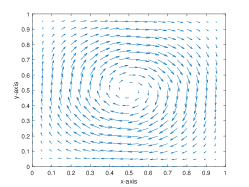
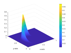
Case 2 FU2019sisc : In this example, the transport of another Gaussian hump in a vortex velocity field is considered. The velocity field is divergence-free, $(c_{1},c_{2})=(\psi_{y},\psi_{x})$ , where $\psi(x,y)=\frac{1}{2}\exp(\sin(\pi x))\exp(\sin(\pi y))$ in the domain. The initial distribution of the Gaussian hump is given as

$\displaystyle u(x,y,t)=\exp\Big{(}-\frac{\left({x}-x_{0}\right)^{2}+\left({y}-y_{0}\right)^{2}}{2\sigma^{2}}\Big{)},$

where the center of the initial Gaussian hump is specified as $x_{0}=0.75$ , $y_{0}=0.5$ and $\sigma^{2}=1.6\times 10^{-3}$ .
•

Case 3 qin2023 : In this case, the initial value is given as

$\displaystyle u_{0}(x,y)=\begin{cases}1,&\text{for }0.1\leq x\leq 0.3,0.1\leq y\leq 0.3,\\ 0,&\text{otherwise. }\end{cases}$

with $\sigma=0.07,x_{0}=y_{0}=0.5$ and the velocity field of $(c_{1},c_{2})=(\sin(\pi y),\sin(\pi x))$ . For simplicity, the periodic boundary condition is employed.

In Case 1, we test the accuracy and property of bound-preserving and mass-preserving of the proposed Strang-ADI-HOC scheme with BP limiter. To illustrate the second-order accuracy in time and the fourth-order accuracy in space at the same time, we set $\tau=h^{2}$ with $\nu=5\times 10^{-3}$ and $T=0.25$ . From Table 5, we can observe that the convergence rate of the Strang-ADI-HOC difference scheme with and without the BP limiter tends to fourth order accuracy. In addition, negative values appear if the BP technique is not applied, and the limiter remedied the negative values in a conservative way. This once again clearly illustrates that the BP technique does not destroy the accuracy when it works, which is consistent with our theoretical result in Remark 3.

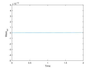
To better observe the effect of the BP technique, we present a series of plots. First, the divergence-free vortex shear and contour plots at the initial time $T=0$ are illustrated in Fig. 11. In Fig. 12, we compare the surface and contour plots without/with the BP limiter and the exact solution with $\nu=5\times 10^{-3},\tau=\frac{h}{6{\max{|f^{\prime}|}}}$ at $T=0.25$ , where $\max{|f^{\prime}|}\approx 4$ . It is clear that the numerical solution calculated without the BP limiter exhibits negative values and oscillations, which pollute the numerical results. In contrast, the numerical solution calculated with the BP limiter shows good consistency with the exact solutions. Finally, the time evolution of the $Mass_{err}$ without/with the BP limiter is plotted in Fig. 13. It is observed that mass conservation is well-preserved numerically in both cases, with or without the BP limiter, which is consistent with our numerical results.

Table 5: Accuracy test with

\nu=5\times 10^{-3},\tau={h}^{2}

	The scheme without the BP limiter					The scheme with the BP limiter
$N$	$L^{2}$ error	Order	$L^{\infty}$ error	Order	$m_{err}$	$L^{2}$ error	Order	$L^{\infty}$ error	Order	$m_{err}$
50	3.9493 E -4	—	3.8901 E -3	—	-8. 9772 E -5	8.0875 E -4	—	6.3116 E -3	—	0
100	1.5794 E -5	4. 64	1.6433 E -4	4. 57	-3.0292 E -12	1.5477 E -5	5. 70	1.5550 E -4	5. 34	0
200	9.4946 E -7	4. 06	9.7788 E -6	4. 07	-3.9502 E -30	9.4946 E -7	4. 03	9.7788 E -6	4. 00	0
300	1.8625 E -7	4. 02	1.9315 E -6	4. 00	-2.1723 E -43	1.8625 E -7	4. 02	1.9315 E -6	4. 00	0

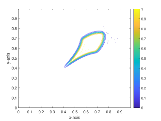
In Case 2, the transport of a Gaussian hump in a vortex velocity field is considered. The velocity field and the initial value distribution are presented in Fig. 14. Fig. 15 and 16 visually compare the contour plots of the moving square wave computed by the HOC-ADI-Splitting scheme without/with the BP limiter at different time. We set $\nu=5\times 10^{-4},N=200$ and $\tau=\frac{h}{4{\max{|f^{\prime}|}}}\leq\frac{h}{6{\max{|f^{\prime}|}}},\max{|f^{\prime}|}=5$ at different time. The distribution solved using a fine mesh of $N=1000$ and $\tau=\frac{h}{6{\max{|f^{\prime}|}}}$ is used as reference for the exact solution. This comparison highlight the growing performance gap: as time progresses, the numerical solution with the BP limiter gets a perfect match with the exact solution, in which the scalar quantity gradually being stretched by the swirling flow over time. In contrast, the solution without the limiter shows significant numerical dissipation of concentration, leading to a less accurate representation of the flow. This example also demonstrates that the condition stated in Theorem 3.2 is sufficient but not necessary for preserving the bound. In practice, the net ratio condition is more lenient and can be effectively applied in actual calculations.

In Case 3, we further test the efficiency of our proposed scheme with different $\nu$ . The space steps are chosen as $N=200$ , and the time steps $\tau=\frac{h}{2{\max{|f^{\prime}|}}}>\frac{h}{6{\max{|f^{\prime}|}}}$ are tested, where ${\max{|f^{\prime}|}}=1$ . The velocity field and the initial value distribution are presented in Fig. 17. In Fig. 18 and 19, we draw the contour plots of the numerical solution calculated by the proposed Strang-ADI-HOC scheme without/with the BP limiter at $T=0.25,0.35$ and 0.5 by setting different $\nu$ . As depicted in Fig. 18, a larger diffusion coefficient of $\nu=10^{-3}$ leads to the rapid dissipation of the square wave over a short time period. In contrast, with a smaller diffusion coefficient of $\nu=10^{-4}$ , the steep gradients at the edges of the square wave persist throughout the dynamic evolution, as illustrated in Fig. 19. Thus, the results with the limiter accurately captures steep fronts without introducing numerical oscillations, even when convection dominates the dynamics.

Example 7

We consider the equation karlsen1997operator

u_{t}+\left(u+(u-0.25)^{3}\right)_{x}-\left(u+u^{2}\right)_{y}=\nu\left(u_{xx}+u_{yy}\right),\\ \quad(x,y,t)\in[-2,5]\times[-2,5]\times[0,1].

with initial data given by

\displaystyle u_{0}(x,y)=\begin{cases}1,&\text{for}(x-0.25)^{2}+(y-2.25)^{2}<0.5\\ 0,&\text{otherwise. }\end{cases}

We set boundary values to zero, which is consistent with the initial data $u_{0}$ . Fig. 20 displays the comparison of three-dimensional views and contour plots between the numerical solution obtained without/with the BP limiter at $T=1$ with $\nu=5\times 10^{-3},N=600,\tau=\frac{h}{{6\max{|f^{\prime}|}}}$ , where $\max{|f^{\prime}|}=2.6875$ . Combining Fig. 20(a) and 20(b), it clearly shows that negative values and non-physical numerical oscillations appear if the BP technique is not applied, while the scheme with the BP limiter leads to accurate positive solutions.

Example 8 We now present an example where we generate approximate solutions to the equation karlsen1997operator ; He2022AFM

u_{t}+f(u)_{x}+g(u)_{y}=\gamma\left(u_{xx}+u_{yy}\right),

with initial data

u_{0}(x,y)=\begin{cases}1,&\text{for }x^{2}+y^{2}<0.5\\ 0,&\text{otherwise}\end{cases}

and $g(u)=\frac{u^{2}}{u^{2}+(1-u)^{2}},$ $f(u)=g(u)\left(1-5(1-u)^{2}\right).$ The flux functions $f$ and $g$ are both "S-shaped" with $f(0)=g(0)=0$ and $f(1)=g(1)=1$ . This problem is motivated from two-phase flow in porous media with a gravitation pull in the $x$ -direction. The computational domain is $[-3,3]\times[-3,3]$ and boundary values are again put equal to zero. We take $N=600,\nu=4\times 10^{-3},\tau=\frac{h}{6\max{|f^{\prime}|}}$ and $T=0.5$ , where $\max{|f^{\prime}|}\approx 3.13$ . We displayed the three-dimensional views and plots of the numerical solution without/with the BP limiter in Fig. 21. No exact solution to this problem is available, but if compared with the numerical solutions reported in karlsen1997operator and He2022AFM , our solutions seem to converge to the correct solution. Thus, our scheme with the limiter provides a highly satisfactory approximation to this model with a nonlinear, degenerate diffusion.

5 Conclusions

In this paper, we have demonstrated that fourth order accurate compact finite difference schemes combined with Strang splitting method for nonlinear convection diffusion problems. A series of theoretical analyses and numerical experiments demonstrate that this improved method effectively optimizes the original algorithm. By decoupling the convection and diffusion terms, the Strang method allows each term to be handled more efficiently, reducing computational constraints and costs. The ADI method’s application to high-dimensional problems ensures that the complexity is manageable, making the method more practical and efficient for real-world applications. Our schemes preserve bound and mass by utilizing the BP limiter proposed by li2018A . To extend the scheme to two-dimensional, we employ ADI method to further reduce the computational cost. Using the properties of the limiter and M-matrix, we give the proof of bound-preserving, mass conservation and stability. Numerical results suggest well performance by the proposed schemes.

References

[1] Acosta C D, Mejia C E. A mollification based operator splitting method for convection diffusion equations. Computers & mathematics with applications, 2010, 59(4): 1397–1408.
[2] Ali A H A, Gardner G A, Gardner L R T. A collocation solution for Burgers equation using cubic B-spline finite elements. Computer Methods in Applied Mechanics and Engineering, 1992, 100:325–337.
[3] Berikelashvili G, Gupta M M, Mirianashvili M. Convergence of fourth order compact difference schemes for three-dimensional convection diffusion equations. SIAM Journal on Numerical Analysis, 2007, 45(1): 443–455.
[4] Bertolazzi E, Manzini G. A second-order maximum principle preserving finite volume method for steady convection diffusion problems. SIAM Journal on Numerical Analysis, 2005, 43(5): 2172–2199.
[5] Chu P C, Fan C. A three-point combined compact difference scheme. Journal of Computational Physics, 1998, 140(2): 370–399.
[6] Douglas J. Alternating direction methods for three space variables. Numerische Mathematik, 1962, 4: 41–63.
[7] Einkemmer L, Ostermann A. Overcoming order reduction in diffusion-reaction splitting. Part 2: Oblique boundary conditions. SIAM Journal on Scientific Computing, 2016, 38(6): A3741–A3757.
[8] Fattah Q N, Hoopes J A. Dispersion in anisotropic, homogeneous, porous media. Journal of Hydraulic Engineering, 1985, 111(5): 810–827.
[9] Genty A, Le Potier C. Maximum and minimum principles for radionuclide transport calculations in geological radioactive waste repository: comparison between a mixed hybrid finite element method and finite volume element discretizations. Transport in porous media, 2011, 88(1): 65–85.
[10] Gottlieb S, Ketcheson D I, Shu C W. High order strong stability preserving time discretizations. Journal of Scientific Computing, 2009, 38(3): 251–289.
[11] He Q, Du W, Shi F, et al. A fast method for solving time-dependent nonlinear convection diffusion problems. Electronic Research Archive, 2022, 30(6): 2165–2182.
[12] Hundsdorfer W H, Verwer J G, Hundsdorfer W H. Numerical solution of time-dependent advection-diffusion-reaction equations. Berlin: Springer, 2003.
[13] Jia H, Li K. A third accurate operator splitting method. Mathematical and computer modelling, 2011, 53(1-2): 387–396.
[14] Kalita J C, Dalal D C, Dass A K. A class of higher order compact schemes for the unsteady two-dimensional convection diffusion equation with variable convection coefficients. International Journal for Numerical Methods in Fluids, 2002, 38(12): 1111–1131.
[15] Karaa S, Zhang J. High order ADI method for solving unsteady convection diffusion problems. Journal of Computational Physics, 2004, 198(1): 1–9.
[16] Karlsen K H, Risebro N H. An operator splitting method for nonlinear convection diffusion equations. Numerische Mathematik, 1997, 77(3): 365–382.
[17] Lee S, Shin J. Energy stable compact scheme for Cahn-Hilliard equation with periodic boundary condition. Computers & Mathematics with Applications, 2019, 77(1): 189–198.
[18] Lele S K. Compact finite difference schemes with spectral-like resolution. Journal of computational physics, 1992, 103(1): 16–42.
[19] Li H, Xie S, Zhang X. A high order accurate bound-preserving compact finite difference scheme for scalar convection diffusion equations. SIAM Journal on Numerical Analysis, 2018, 56(6): 3308–3345.
[20] Mohebbi A, Dehghan M. High-order compact solution of the one-dimensional heat and advection-diffusion equations. Applied mathematical modelling, 2010, 34(10): 3071–3084.
[21] Parlange J Y. Water transport in soils. Annual review of fluid mechanics, 1980, 12(1): 77–102.
[22] Peaceman D W. Fundamentals of Numerical Reservoir Simulation. Elsevier, 2000.
[23] Peaceman D W, Rachford, Jr H H. The numerical solution of parabolic and elliptic differential equations. Journal of the Society for industrial and Applied Mathematics, 1955, 3(1): 28–41.
[24] Plemmons R J. M-matrix characterizations. I-nonsingular M-matrices. Linear Algebra and its applications, 1977, 18(2): 175–188.
[25] Poole G, Boullion T. A survey on M-matrices. SIAM review, 1974, 16(4): 419–427.
[26] Rui H, Tabata M. A mass-conservative characteristic finite element scheme for convection diffusion problems. Journal of Scientific Computing, 2010, 43: 416–432.
[27] Shen J, Zhang X. Discrete maximum principle of a high order finite difference scheme for a generalized Allen-Cahn equation. Communications in Mathematical Sciences, 2022, 20(5): 1409–1436.
[28] Shu C W, Osher S. Efficient implementation of essentially non-oscillatory shock-capturing schemes. Journal of computational physics, 1988, 77(2): 439–471.
[29] Srinivasan S, Poggie J, Zhang X. A positivity-preserving high order discontinuous Galerkin scheme for convection diffusion equations. Journal of Computational Physics, 2018, 366: 120–143.
[30] Strang G. On the construction and comparison of difference schemes. SIAM journal on numerical analysis, 1968, 5(3): 506–517.
[31] Tian Z F. A rational high-order compact ADI method for unsteady convection diffusion equations. Computer Physics Communications, 2011, 182(3): 649–662.
[32] Tian Z F, Ge Y B. A fourth-order compact ADI method for solving two-dimensional unsteady convection diffusion problems. Journal of Computational and Applied Mathematics, 2007, 198(1): 268–286.
[33] van der Vegt J J W, Xia Y, Xu Y. Positivity preserving limiters for time-implicit higher order accurate discontinuous Galerkin discretizations. SIAM journal on scientific computing, 2019, 41(3): A2037–A2063.
[34] Wang H, Shu C W, Zhang Q. Stability and error estimates of local discontinuous Galerkin methods with implicit-explicit time-marching for advection-diffusion problems. SIAM Journal on Numerical Analysis, 2015, 53(1): 206–227.
[35] Wang T. New characteristic difference method with adaptive mesh for one-dimensional unsteady convection-dominated diffusion equations. International Journal of Computer Mathematics, 2005, 82(10): 1247–1260.
[36] Wang Y M. Fourth-order compact finite difference methods and monotone iterative algorithms for quasi-linear elliptic boundary value problems. SIAM Journal on Numerical Analysis, 2015, 53(2): 1032–1057.
[37] Xie S S, Heo S, Kim S, Woo G, Yi S. Numerical solution of one-dimensional Burgers equation using reproducing kernel function. J. Comput. Appl. Math., 2008, 214(2): 417–434.
[38] Xiong T, Qiu J M, Xu Z. High order maximum-principle-preserving discontinuous Galerkin method for convection diffusion equations. SIAM Journal on Scientific Computing, 2015, 37(2): A583–A608.
[39] Zhang L, Ge Y. Numerical solution of nonlinear advection diffusion reaction equation using high-order compact difference method. Applied Numerical Mathematics, 2021, 166: 127–145.
[40] Zhang L, Ge Y, Wang Z. Positivity-preserving high-order compact difference method for the Keller-Segel chemotaxis model. Mathematical Biosciences and Engineering, 2022, 19(7): 6764–6794.
[41] Zhang X, Liu Y, Shu C W. Maximum-principle-satisfying high order finite volume weighted essentially nonoscillatory schemes for convection diffusion equations. SIAM Journal on Scientific Computing, 2012, 34(2): A627–A658.
[42] Zhuang C, Zeng R. A positivity-preserving scheme for the simulation of streamer discharges in non-attaching and attaching gases. Communications in Computational Physics, 2014, 15(1): 153–178.
[43] Zlatev Z, Berkowicz R, Prahm L P. Implementation of a variable stepsize variable formula method in the time-integration part of a code for treatment of long-range transport of air pollutants. Journal of Computational Physics, 1984, 55(2): 278-301.
[44] Kaya D. An explicit solution of coupled Burgers equations by decomposition method. International Journal of Mathematics and Mathematical Sciences, 2001, 27: 675-680.
[45] Fu K, Liang D. The time second order mass conservative characteristic FDM for advection–diffusion equations in high dimensions. Journal of Scientific Computing, 2017, 73: 26-49.
[46] Fu K, Liang D. A mass-conservative temporal second order and spatial fourth order characteristic finite volume method for atmospheric pollution advection diffusion problems. SIAM Journal on Scientific Computing, 2019, 41(6): B1178-B1210.
[47] Liao H L, Sun Z Z. Maximum norm error bounds of ADI and compact ADI methods for solving parabolic equations. Numerical Methods for Partial Differential Equations, 2010,26:37-60.
[48] Shen J, Tang T, Yang J. On the maximum principle preserving schemes for the generalized Allen–Cahn equation. Communications in Mathematical Sciences, 2016, 14(6): 1517-1534.
[49] Hundsdorfer W, Verwer J. Numerical Solution of Time-Dependent Advection-Diffusion-Reaction Equations. Heidelberg: Springer, 2003.
[50] Wang Y, Xie S S, Fu H F. Efficient, linearized high-order compact difference schemes for nonlinear parabolic equations I: One-dimensional problem. Numerical Methods for Partial Differential Equations, 2023, 39(2): 1529-1557.
[51] Zhang J, Sun H, Zhao J J. High order compact scheme with multigrid local mesh refinement procedure for convection diffusion problems. Computer Methods in Applied Mechanics and Engineering, 2002, 191(41-42): 4661-4674.
[52] Ito K, Qiao Z. A high order compact MAC finite difference scheme for the Stokes equations: augmented variable approach. Journal of Computational Physics, 2008, 227(17): 8177-8190.
[53] Cockburn B, Shu C W. Nonlinearly stable compact schemes for shock calculations. SIAM Journal on Numerical Analysis, 1994, 31(3): 607–627.
[54] Li H, Zhang X X. A high order accurate bound-preserving compact finite difference scheme for two-dimensional incompressible flow. Communications on Applied Mathematics and Computation, 2024, 6(1): 113-141.
[55] Qin D, Fu K, Liang D. Positivity preserving temporal second-order spatial fourth-order conservative characteristic methods for convection dominated diffusion equations. Computers & Mathematics with Applications, 2023, 149: 190-202.