Fractional quantum Hall effect at
Abstract
Motivated by two independent experiments revealing a resistance minimum at the Landau level (LL) filling factor , characteristic of the fractional quantum Hall effect (FQHE) and suggesting electron condensation into a yet unknown quantum liquid, we propose that this state likely belongs in a parton sequence, put forth recently to understand the emergence of FQHE at . While the state proposed here directly follows three simpler parton states, all known to occur in the second LL, it is topologically distinct from the Jain composite fermion (CF) state which occurs at the same filling of the lowest LL. We predict experimentally measurable properties of the parton state that can reveal its underlying topological structure and definitively distinguish it from the Jain CF state.
pacs:
73.43-f, 71.10.PmThe fractional quantum Hall effect (FQHE) Tsui et al. (1982); Laughlin (1983) forms a paradigm in our understanding of strongly correlated quantum phases of matter. Of particular interest among the panoply of FQHE phases are the ones observed in the second Landau level (SLL) of ordinary semiconductors such as GaAs. These have attracted widespread attention because of the possibility that the excitations of these phases obey non-Abelian braiding statistics, which could potentially be utilized in carrying out fault-tolerant topological quantum computation Kitaev (2003); Nayak et al. (2008).
FQHE was first observed at filling factor Tsui et al. (1982) in the lowest LL (LLL) and was explained by Laughlin using his eponymous wave function Laughlin (1983). Soon a whole zoo of fractions were observed, primarily along the sequence ( and are positive integers) and its particle-hole conjugate Eisenstein et al. (1990). These FQHE states can be understood as arising from the integer quantum Hall effect (IQHE) of composite fermions (CFs) Jain (1989a, 2007), which are bounds states of electron and an even number () of quantized vortices. The theory of weakly interacting CFs captures almost all of the observed FQHE phenomenology in the LLL.
In comparison to the FQHE in the LLL, the FQH states in the SLL are fewer in number and are more fragile Willett et al. (1987). Moreover, the nature of many FQH states in the SLL is dramatically different from their LLL counterparts. In particular, one of the strongest FQH states in the SLL occurs at Willett et al. (1987), whereas at the corresponding half-filled LLL a compressible state is observed. A key breakthrough in the field of FQHE came about by a proposal of Moore and Read Moore and Read (1991), who posited a “Pfaffian” wave function to describe the state at . Subsequently, it was understood that the Pfaffian wave function can be interpreted as a -wave paired state of composite fermions Read and Green (2000). The excitations of the Pfaffian state are Majorana fermions which, owing to their non-Abelian braiding properties, could form building blocks of a topological quantum computer Kitaev (2003); Nayak et al. (2008).
The nature of the state at state in the SLL, although believed to be Laughlin-like, has been under intense debate d’Ambrumenil and Reynolds (1988); Balram et al. (2013); Johri et al. (2014); Peterson et al. (2015); Kleinbaum et al. (2015); Jeong et al. (2017); Balram et al. (2020). FQHE has been observed at Xia et al. (2004); Choi et al. (2008); Pan et al. (2008); Kumar et al. (2010) but is widely believed to be of a parafermionic nature, unlike the Abelian LLL Jain CF state at Read and Rezayi (1999); Rezayi and Read (2009); Wójs (2009); Bonderson et al. (2012); Sreejith et al. (2013); Zhu et al. (2015); Mong et al. (2017); Pakrouski et al. (2016). Furthermore, as yet there is no conclusive experimental evidence of FQHE at the next three members of the Jain sequence, namely , , and , in the SLL Shingla et al. (2018), though some features of FQHE have been reported in the literature at some of these fillings Pan et al. (2008); Choi et al. (2008); Reichl et al. (2014) (A non-Abelian parton state at was constructed in Ref. Faugno et al. (2020) and shown to be feasible in the SLL.). However, FQHE has been observed at Kumar et al. (2010). These observations collectively point to the fact that the nature of FQHE states in the LLL and SLL are different from each other, and a description of FQHE states in the SLL likely entails going beyond the framework of noninteracting composite fermions.
Recently, candidate “parton” states have been constructed to describe the FQHE at many of the experimentally observed fillings in the SLL Balram et al. (2018a, b, 2019). The parton theory Jain (1989b) produces model incompressible states beyond the Laughlin Laughlin (1983) and the CF theory Jain (1989a). The “” parton states for give a good description of the SLL FQHE states observed at and Balram et al. (2018a, b). In particular, the sequence underscores the unusual stability of in the SLL.
In this work, we consider the next member of the parton sequence, namely and consider its feasibility at . While FQHE at has not been established conclusively, indications for it in the form of a minimum in the longitudinal resistance have already been seen in experiments Choi et al. (2008); Reichl et al. (2014). Future experiments on high-quality samples could likely establish FQHE at this filling by an observation of a well-quantized plateau in the Hall resistance. We show that the parton state gives a good description of the exact SLL Coulomb ground state seen in numerics. Furthermore, the parton state is energetically favorable compared to the Jain CF state at in the thermodynamic limit. Therefore, if FQHE is established at , it is highly likely to be distinct from its LLL counterpart at , which is well described by the Jain CF state. The parton state is topologically distinct from the Jain CF state and we make predictions for experimentally measurable quantities that can unambiguously distinguish the two. In particular, the parton state supports counter-propagating edge modes that do not occur in the Jain CF state.
The parton theory put forth by Jain Jain (1989b) constructs FQHE states as a product of IQH states. The essential idea is to break each electron into fictitious objects called partons, place the partons into incompressible IQH states, and recover the final state by fusing the partons back into the physical electrons. The -electron wave function for the -parton Jain state, denoted as “”, is given by
| (1) |
Here is the two-dimensional coordinate of electron which is parametrized as a complex number, denotes the parton species and implements projection into the LLL. Each parton species is exposed to the external magnetic field and occupies the same area, which fixes the charge of the parton species to , with , where is the charge of the electron. The state is the Slater determinant IQH wave function of electrons filling the lowest LLs. We allow for and negative values are denoted by , with . The parton state of Eq. (1) occurs at a filling factor of and has a shift Wen and Zee (1992) of in the spherical geometry.
The Laughlin state Laughlin (1983) is a “” parton state. The parton state () with wave function () correspond to the Jain CF states Jain (1989a). Recently, it has been shown that parton states of the form “” which are not composite fermion states, could be viable candidates to describe certain FQH states observed in the LLL in wide quantum wells Faugno et al. (2019) and in LLs of graphene Wu et al. (2017); Kim et al. (2019).
The motivation for considering the parton state stems from the recent application of parton theory to capture states in the SLL Balram et al. (2018a, b, 2019). Consider the family of parton states described by the wave function
| (2) |
The sign in Eq. (2) indicates that the states written at both sides of the sign differ slightly in the details of the projection. We expect that such details do not change the topological nature of the states Balram and Jain (2016). Throughout this text, for the parton states we use the form given on the rightmost side of Eq. (2). A nice feature of the parton wave functions stated in Eq. (2) is that they can be evaluated for large system sizes which allow a reliable extrapolation of their thermodynamic energies. One can construct the above parton states for large system sizes because the constituent Jain CF states can be evaluated for hundreds of electrons using the Jain-Kamilla method of projection Jain and Kamilla (1997); Möller and Simon (2005); Jain (2007); Davenport and Simon (2012); Balram et al. (2015a). The Jain CF states in this work are evaluated using the Jain-Kamilla method.
The member, namely , is likely topologically equivalent to the Jain CF state Balram and Jain (2016). The member has a good overlap with the exact SLL Coulomb ground state at Balram et al. (2018a). The state, , gives a good description of the Coulomb ground state at Balram et al. (2018b). In the Supplemental Material (SM) SM we provide further evidence in favor of the feasibility of the parton state to describe the FQHE. We shall consider the member of this sequence which occurs at filling factor .
Although there is no definitive observation of FQHE at in the SLL, signatures of incompressibility have been seen at and its particle-hole conjugate at Choi et al. (2008); Reichl et al. (2014). FQHE at is likely swamped by a bubble phase Shingla et al. (2018); however, it is likely that with improvements in the sample quality or for some interaction parameters close to that of the SLL Coulomb one, FQHE will ultimately be observed at .
For all our calculations, we deploy Haldane’s spherical geometry Haldane (1983), in which electrons reside on the surface of a sphere in the presence of a radial magnetic field generated by a monopole of strength located at the center of the sphere. FQHE ground states occur at flux values , where is a rational number called the shift, which is useful in characterizing the topological nature of the FQHE state Wen and Zee (1992). All FQHE ground states are uniform on the sphere and thus have total orbital angular momentum . The parton states of Eq. (2) satisfy the flux-particle relationship ; i.e., their filling factors are and their shifts are . Of particular interest to us in this work is the parton state which has a shift of . This parton state is topologically distinct from the Jain CF state which also occurs at but has a shift of . We assume a single-component system and neglect the effects of LL mixing and disorder. Under these assumptions, states related by particle-hole conjugation are considered on the same footing.
Throughout this work, we shall write wave functions in the LLL, which is where they are easily evaluated, even though they might apply to states occurring in the SLL. Haldane Haldane (1983) showed that the physics of the SLL can be simulated in the LLL by using an effective interaction that has the same set of Haldane pseudopotentials in the LLL as the Coulomb interaction has in the SLL. In this work, we have used the form of the effective interaction described in Ref. Shi et al. (2008) to simulate the physics of the SLL in the LLL.
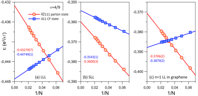
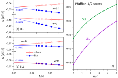
Let us begin by testing the viability of the parton state for FQHE. In Fig. 1 we compare the energies of the parton and the Jain CF states at in the LLL and the SLL. In the LLL, as expected, we find that the Jain CF state has lower energy than the parton state. However, in the SLL we find that the parton state is energetically more favorable compared to the Jain CF state. For the sake of completeness, we have also investigated the competition between the parton and Jain CF states in the LL of monolayer graphene. The effective interaction we use to simulate the physics of the LL of monolayer graphene in the LLL is described in Ref. Balram et al. (2015b). We find the Jain CF state has lower energy here, consistent with the fact that experimentally observed FQHE states in the LL of monolayer graphene are well described by the CF paradigm Amet et al. (2015); Balram et al. (2015b); Zeng et al. (2019). Results for LL of graphene are identical to those in the LLL of GaAs under our working assumptions of neglecting effects of finite width and LL mixing.
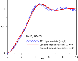
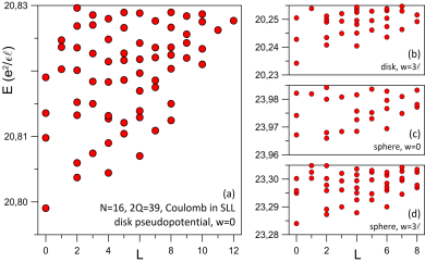
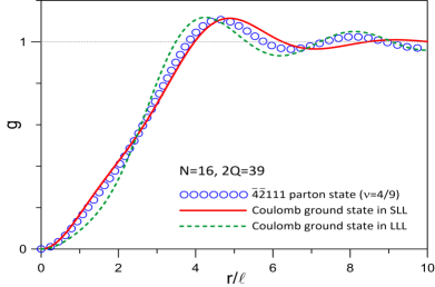
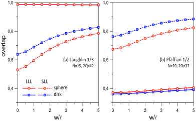
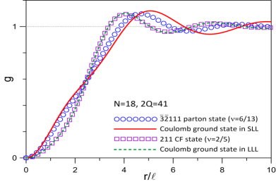
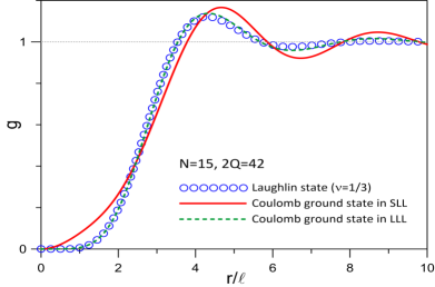
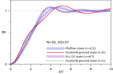
Next, we turn to comparisons of the parton state with the exact SLL Coulomb ground state. The smallest system accessible to exact diagonalization (ED) is that of electrons at a flux of which has a Hilbert space dimension of . We have evaluated the ground state for this system with the truncated pseudopotentials from the disk geometry, which differ slightly from the spherical pseudopotentials but are known to provide a more reliable extrapolation to the thermodynamic limit Peterson et al. (2008a, b). The exact SLL Coulomb ground obtained by using the truncated disk pseudopotentials has . In Fig. 2 we compare the pair-correlation function foo of this exact SLL Coulomb ground state with that of the parton state. Both these pair-correlation functions show oscillations that decay at long distances, which is a typical characteristic of incompressible states Kamilla et al. (1997); Balram et al. (2015c). Moreover, the two pair-correlation functions are in reasonable agreement with each other. For completeness, we have also evaluated the exact LLL Coulomb ground state for the same system. The overlaps of the LLL and SLL Coulomb ground states obtained using the disk pseudopotentials is and their pair-correlation functions are also very different from each other SM which indicate that the nature of the ground state in the two LLs are very different.
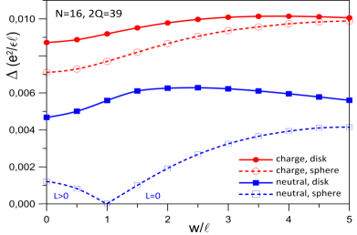
Currently, we do not have a reliable estimate of the thermodynamic values of the gaps predicted by our parton ansatz. However, we can extract the charge and neutral gaps for particles from exact diagonalization of the SLL Coulomb interaction at the parton shift. The charge gap here is defined as , where is the exact ground state energy at flux and the factor of in the denominator accounts for the fact that the addition of a single flux quantum in the parton state produces four fundamental quasiholes. The neutral gap is defined as the difference between the two lowest exact energies at the flux of . The charge and neutral gaps for , evaluated using exact diagonalization with the disk pseudopotentials, are and respectively, where is the magnetic length and is the dielectric constant of the background host material.
We next consider the effect of finite width on the system, which we model by taking the transverse wave function to be the ground state for an infinite square quantum well of width (see SM SM for details). For the disk pseudopotentials, we find that the ground state for electrons has for (at least) SM . Moreover, the pair-correlation function of the exact ground state agrees well with that of the parton state for the entire range of widths considered in this work (see Fig. 2 and Ref. SM ). Furthermore, we find that the system has robust charge and neutral gaps for all the widths considered. We note that the ground state is delicate. In particular, the exact SLL Coulomb ground state obtained using the spherical pseudopotentials has . However, the overlap between the lowest energy state obtained using the spherical pseudopotentials and the ground state obtained using the disk pseudopotentials is , which indicates that these two states are close to each other. Encouragingly, with the spherical pseudopotentials, as the quantum well width is increased the ground state turns uniform in the range and stays uniform for SM . These results indicate that finite thickness enhances the stability of the parton state.
Now that we have made a case for the plausibility of the parton state to occur in the SLL, we shall turn to deduce the experimental consequences of this parton ansatz. An additional particle in the factor has charge , whereas that in the factors and has a charge and respectively. All the quasiparticles of the parton state obey Abelian braid statistics Wen (1991). The Jain CF state is also an Abelian state and hosts quasiparticles of charge and .
Next, to infer other topological consequences of the ansatz, we consider the low-energy effective theory of its edge, which is described by the Lagrangian density WEN (1991); Wen (1992, 1995); Moore and Wen (1998):
| (3) |
Here is the fully anti-symmetric Levi-Civita tensor, is the vector potential corresponding to the external electromagnetic field, is the internal gauge field, and we have used the Einstein’s convention of summing repeated indices. The integer-valued symmetric matrix and the charge vector of Eq. (3) for the parton state are given by (see SM SM for a derivation)
| (4) |
The above matrix has four negative and one positive eigenvalues and thus the state hosts four upstream and one downstream edge modes. A naive counting suggests that there are a total of nine edge states for the ansatz: four from the factor , two from , and one from each factor of . However, these edges states are not all independent since the density variations of the five partons must be identified. This results in four constraints and leads to five edge states consistent with that ascertained from the above matrix.
Assuming full equilibration of the edge modes, the thermal Hall conductance at temperatures much smaller than the gap takes a quantized value proportional to the chiral central charge , which is defined as the difference in the number of downstream and upstream modes: Kane and Fisher (1997). For ansatz, we thus predict a thermal Hall conductance of . The Hall viscosity of the state is also expected to be quantized Read (2009): , where is the electron density and is the shift of the parton state. The ground-state degeneracy of the parton state on a topologically nontrivial manifold with genus is . Besides the parton states Balram et al. (2020), the ansatz provides another example of a fully spin polarized Abelian FQH state at (with coprime), which has a ground state degeneracy on the torus that is greater than .
The Jain CF state is described by the matrix , where is the matrix of all ones and is the identity matrix, and charge vector . In contrast to the state, assuming the absence of edge reconstruction, the Jain CF state has four downstream edge states and no upstream modes. The Jain CF state thus has a thermal Hall conductance of . Moreover, the Hall viscosity of the Jain CF state is given by , corresponding to shift . On a manifold of genus , the Jain CF state has a degeneracy of .
The presence of upstream neutral modes can be detected in shot noise experiments Bid et al. (2010); Dolev et al. (2011); Gross et al. (2012); Inoue et al. (2014). Recently, thermal Hall measurements have been carried out at several filling factors in the lowest as well as the second LL Banerjee et al. (2017, 2018); Srivastav et al. (2019). These experiments can be used to test the predictions of the parton theory and therefore can unambiguously distinguish between the topological nature of the 4/9 states in the SLL and the LLL. In particular, including the contributions of the filled LLLs of spin up and spin down, the thermal Hall conductance of the state in the SLL is which is different from what one would expect from the Jain CF state in the SLL, which has .
In summary, we have considered the viability of the “” parton state for FQHE at where the first signs of incompressibility in the form of minimum in longitudinal resistance have already been observed experimentally Choi et al. (2008); Reichl et al. (2014). Interestingly, if FQHE eventually stabilizes at this filling factor, then it is likely to be topologically different from its LLL counterpart at , which is described by a Jain CF state. We also proposed experimental measurements that can reveal the underlying topological structure of the parton state and decisively distinguish it from the state occurring in the lowest Landau level.
Acknowledgements.
We acknowledge useful discussions with Maissam Barkeshli, Jainendra K. Jain, Mark S. Rudner, Dam T. Son, and Bo Yang. This work was supported by the Polish NCN Grant No. 2014/14/A/ST3/00654 (A. W.). We thank Wrocław Centre for Networking and Supercomputing and Academic Computer Centre CYFRONET, both parts of PL-Grid Infrastructure. Some of the numerical calculations reported in this work were carried out on the Nandadevi supercomputer, which is maintained and supported by the Institute of Mathematical Science’s High-Performance Computing Center. This research was supported in part by the International Centre for Theoretical Sciences (ICTS) during a visit for the program Novel Phases of Quantum Matter (code: ICTS/topmatter2019/12)References
- Tsui et al. (1982) D. C. Tsui, H. L. Stormer, and A. C. Gossard, Phys. Rev. Lett. 48, 1559 (1982).
- Laughlin (1983) R. B. Laughlin, Phys. Rev. Lett. 50, 1395 (1983).
- Kitaev (2003) A. Kitaev, Annals of Physics 303, 2 (2003).
- Nayak et al. (2008) C. Nayak, S. H. Simon, A. Stern, M. Freedman, and S. Das Sarma, Rev. Mod. Phys. 80, 1083 (2008).
- Eisenstein et al. (1990) J. P. Eisenstein, H. L. Stormer, L. N. Pfeiffer, and K. W. West, Phys. Rev. B 41, 7910 (1990).
- Jain (1989a) J. K. Jain, Phys. Rev. Lett. 63, 199 (1989a).
- Jain (2007) J. K. Jain, Composite Fermions (Cambridge University Press, New York, US, 2007).
- Willett et al. (1987) R. Willett, J. P. Eisenstein, H. L. Störmer, D. C. Tsui, A. C. Gossard, and J. H. English, Phys. Rev. Lett. 59, 1776 (1987).
- Moore and Read (1991) G. Moore and N. Read, Nucl. Phys. B 360, 362 (1991).
- Read and Green (2000) N. Read and D. Green, Phys. Rev. B 61, 10267 (2000).
- d’Ambrumenil and Reynolds (1988) N. d’Ambrumenil and A. M. Reynolds, Journal of Physics C: Solid State Physics 21, 119 (1988).
- Balram et al. (2013) A. C. Balram, Y.-H. Wu, G. J. Sreejith, A. Wójs, and J. K. Jain, Phys. Rev. Lett. 110, 186801 (2013).
- Johri et al. (2014) S. Johri, Z. Papić, R. N. Bhatt, and P. Schmitteckert, Phys. Rev. B 89, 115124 (2014).
- Peterson et al. (2015) M. R. Peterson, Y.-L. Wu, M. Cheng, M. Barkeshli, Z. Wang, and S. Das Sarma, Phys. Rev. B 92, 035103 (2015).
- Kleinbaum et al. (2015) E. Kleinbaum, A. Kumar, L. N. Pfeiffer, K. W. West, and G. A. Csáthy, Phys. Rev. Lett. 114, 076801 (2015).
- Jeong et al. (2017) J.-S. Jeong, H. Lu, K. H. Lee, K. Hashimoto, S. B. Chung, and K. Park, Phys. Rev. B 96, 125148 (2017).
- Balram et al. (2020) A. C. Balram, J. K. Jain, and M. Barkeshli, Phys. Rev. Research 2, 013349 (2020).
- Xia et al. (2004) J. S. Xia, W. Pan, C. L. Vicente, E. D. Adams, N. S. Sullivan, H. L. Stormer, D. C. Tsui, L. N. Pfeiffer, K. W. Baldwin, and K. W. West, Phys. Rev. Lett. 93, 176809 (2004).
- Choi et al. (2008) H. C. Choi, W. Kang, S. Das Sarma, L. N. Pfeiffer, and K. W. West, Phys. Rev. B 77, 081301 (2008).
- Pan et al. (2008) W. Pan, J. S. Xia, H. L. Stormer, D. C. Tsui, C. Vicente, E. D. Adams, N. S. Sullivan, L. N. Pfeiffer, K. W. Baldwin, and K. W. West, Phys. Rev. B 77, 075307 (2008).
- Kumar et al. (2010) A. Kumar, G. A. Csáthy, M. J. Manfra, L. N. Pfeiffer, and K. W. West, Phys. Rev. Lett. 105, 246808 (2010).
- Read and Rezayi (1999) N. Read and E. Rezayi, Phys. Rev. B 59, 8084 (1999).
- Rezayi and Read (2009) E. H. Rezayi and N. Read, Phys. Rev. B 79, 075306 (2009).
- Wójs (2009) A. Wójs, Phys. Rev. B 80, 041104 (2009).
- Bonderson et al. (2012) P. Bonderson, A. E. Feiguin, G. Möller, and J. K. Slingerland, Phys. Rev. Lett. 108, 036806 (2012).
- Sreejith et al. (2013) G. J. Sreejith, Y.-H. Wu, A. Wójs, and J. K. Jain, Phys. Rev. B 87, 245125 (2013).
- Zhu et al. (2015) W. Zhu, S. S. Gong, F. D. M. Haldane, and D. N. Sheng, Phys. Rev. Lett. 115, 126805 (2015).
- Mong et al. (2017) R. S. K. Mong, M. P. Zaletel, F. Pollmann, and Z. Papić, Phys. Rev. B 95, 115136 (2017).
- Pakrouski et al. (2016) K. Pakrouski, M. Troyer, Y.-L. Wu, S. Das Sarma, and M. R. Peterson, Phys. Rev. B 94, 075108 (2016).
- Shingla et al. (2018) V. Shingla, E. Kleinbaum, A. Kumar, L. N. Pfeiffer, K. W. West, and G. A. Csáthy, Phys. Rev. B 97, 241105 (2018).
- Reichl et al. (2014) C. Reichl, J. Chen, S. Baer, C. Rössler, T. Ihn, K. Ensslin, W. Dietsche, and W. Wegscheider, New Journal of Physics 16, 023014 (2014).
- Faugno et al. (2020) W. N. Faugno, J. K. Jain, and A. C. Balram, Phys. Rev. Research 2, 033223 (2020).
- Balram et al. (2018a) A. C. Balram, M. Barkeshli, and M. S. Rudner, Phys. Rev. B 98, 035127 (2018a).
- Balram et al. (2018b) A. C. Balram, S. Mukherjee, K. Park, M. Barkeshli, M. S. Rudner, and J. K. Jain, Phys. Rev. Lett. 121, 186601 (2018b).
- Balram et al. (2019) A. C. Balram, M. Barkeshli, and M. S. Rudner, Phys. Rev. B 99, 241108 (2019).
- Jain (1989b) J. K. Jain, Phys. Rev. B 40, 8079 (1989b).
- Wen and Zee (1992) X. G. Wen and A. Zee, Phys. Rev. Lett. 69, 953 (1992).
- Faugno et al. (2019) W. N. Faugno, A. C. Balram, M. Barkeshli, and J. K. Jain, Phys. Rev. Lett. 123, 016802 (2019).
- Wu et al. (2017) Y. Wu, T. Shi, and J. K. Jain, Nano Letters 17, 4643 (2017), pMID: 28649831, eprint http://dx.doi.org/10.1021/acs.nanolett.7b01080.
- Kim et al. (2019) Y. Kim, A. C. Balram, T. Taniguchi, K. Watanabe, J. K. Jain, and J. H. Smet, Nature Physics 15, 154 (2019).
- Balram and Jain (2016) A. C. Balram and J. K. Jain, Phys. Rev. B 93, 235152 (2016).
- Jain and Kamilla (1997) J. K. Jain and R. K. Kamilla, Phys. Rev. B 55, R4895 (1997).
- Möller and Simon (2005) G. Möller and S. H. Simon, Phys. Rev. B 72, 045344 (2005).
- Davenport and Simon (2012) S. C. Davenport and S. H. Simon, Phys. Rev. B 85, 245303 (2012).
- Balram et al. (2015a) A. C. Balram, C. Töke, A. Wójs, and J. K. Jain, Phys. Rev. B 92, 075410 (2015a).
- (46) See Supplemental Material (SM) accompanying this paper for (i) a derivation of the low-energy effective edge theory of the parton state and (ii) a detailed study of the effect of finite width at and (iii) a comparison of candidate states with exact Coulomb ground states at other filling factors, namely and , in the second Landau level. The SM includes Refs. Morf (1998); Wójs (2009); Hutasoit et al. (2017); Zuo et al. (2020).
- Haldane (1983) F. D. M. Haldane, Phys. Rev. Lett. 51, 605 (1983).
- Shi et al. (2008) C. Shi, S. Jolad, N. Regnault, and J. K. Jain, Phys. Rev. B 77, 155127 (2008).
- Balram et al. (2015b) A. C. Balram, C. Tőke, A. Wójs, and J. K. Jain, Phys. Rev. B 92, 205120 (2015b).
- Amet et al. (2015) F. Amet, A. J. Bestwick, J. R. Williams, L. Balicas, K. Watanabe, T. Taniguchi, and D. Goldhaber-Gordon, Nat. Commun. 6, 5838 (2015).
- Zeng et al. (2019) Y. Zeng, J. I. A. Li, S. A. Dietrich, O. M. Ghosh, K. Watanabe, T. Taniguchi, J. Hone, and C. R. Dean, Phys. Rev. Lett. 122, 137701 (2019).
- Morf et al. (1986) R. Morf, N. d’Ambrumenil, and B. I. Halperin, Phys. Rev. B 34, 3037 (1986).
- Balram and Jain (2017) A. C. Balram and J. K. Jain, Phys. Rev. B 96, 235102 (2017).
- Peterson et al. (2008a) M. R. Peterson, T. Jolicoeur, and S. Das Sarma, Phys. Rev. Lett. 101, 016807 (2008a).
- Peterson et al. (2008b) M. R. Peterson, T. Jolicoeur, and S. Das Sarma, Phys. Rev. B 78, 155308 (2008b).
- (56) We compare the pair-correlation functions since, due to technical reasons, it has not yet been possible to calculate the overlap of the parton state with the state obtained from exact diagonalization for the large system size considered in this work.
- Kamilla et al. (1997) R. K. Kamilla, J. K. Jain, and S. M. Girvin, Phys. Rev. B 56, 12411 (1997).
- Balram et al. (2015c) A. C. Balram, C. Tőke, and J. K. Jain, Phys. Rev. Lett. 115, 186805 (2015c).
- Wen (1991) X. G. Wen, Phys. Rev. Lett. 66, 802 (1991).
- WEN (1991) X. WEN, Modern Physics Letters B 05, 39 (1991).
- Wen (1992) X.-G. Wen, International Journal of Modern Physics B 06, 1711 (1992).
- Wen (1995) X.-G. Wen, Advances in Physics 44, 405 (1995).
- Moore and Wen (1998) J. E. Moore and X.-G. Wen, Phys. Rev. B 57, 10138 (1998).
- Kane and Fisher (1997) C. L. Kane and M. P. A. Fisher, Phys. Rev. B 55, 15832 (1997).
- Read (2009) N. Read, Phys. Rev. B 79, 045308 (2009).
- Bid et al. (2010) A. Bid, N. Ofek, H. Inoue, M. Heiblum, C. L. Kane, V. Umansky, and D. Mahalu, Nature 466, 585 (2010).
- Dolev et al. (2011) M. Dolev, Y. Gross, R. Sabo, I. Gurman, M. Heiblum, V. Umansky, and D. Mahalu, Phys. Rev. Lett. 107, 036805 (2011).
- Gross et al. (2012) Y. Gross, M. Dolev, M. Heiblum, V. Umansky, and D. Mahalu, Phys. Rev. Lett. 108, 226801 (2012).
- Inoue et al. (2014) H. Inoue, A. Grivnin, Y. Ronen, M. Heiblum, V. Umansky, and D. Mahalu, Nature Communications 5, 4067 (2014).
- Banerjee et al. (2017) M. Banerjee, M. Heiblum, A. Rosenblatt, Y. Oreg, D. E. Feldman, A. Stern, and V. Umansky, Nature 545, 75+ (2017).
- Banerjee et al. (2018) M. Banerjee, M. Heiblum, V. Umansky, D. E. Feldman, Y. Oreg, and A. Stern, Nature 559, 205 (2018).
- Srivastav et al. (2019) S. K. Srivastav, M. R. Sahu, K. Watanabe, T. Taniguchi, S. Banerjee, and A. Das, Science Advances 5 (2019), eprint https://advances.sciencemag.org/content/5/7/eaaw5798.full.pdf.
- Morf (1998) R. H. Morf, Phys. Rev. Lett. 80, 1505 (1998).
- Hutasoit et al. (2017) J. A. Hutasoit, A. C. Balram, S. Mukherjee, Y.-H. Wu, S. S. Mandal, A. Wójs, V. Cheianov, and J. K. Jain, Phys. Rev. B 95, 125302 (2017).
- Kuśmierz and Wójs (2018) B. Kuśmierz and A. Wójs, Phys. Rev. B 97, 245125 (2018).
- Scarola et al. (2002) V. W. Scarola, S.-Y. Lee, and J. K. Jain, Phys. Rev. B 66, 155320 (2002).
- Pakrouski et al. (2015) K. Pakrouski, M. R. Peterson, T. Jolicoeur, V. W. Scarola, C. Nayak, and M. Troyer, Phys. Rev. X 5, 021004 (2015).
- Zuo et al. (2020) Z.-W. Zuo, A. C. Balram, S. Pu, J. Zhao, A. Wójs, and J. K. Jain, arXiv e-prints arXiv:2002.09356 (2020), eprint 2002.09356.
Supplemental Material for “Fractional Quantum Hall Effect at ”
In this Supplemental Material (SM) we provide
I Derivation of the low-energy effective theory of the parton edge
To derive the low-energy effective theory of the parton edge we closely follow the procedure outlined in the Supplemental Material of Ref. Balram et al. (2018b). We are interested in the member of the parton sequence. We shall first discuss the case of general and then specialize to the case of . The unprojected wave function of the parton state can be re-written as
| (S1) |
where is the Slater determinant state of filled Landau levels and is the Laughlin state Laughlin (1983). This state can be expressed in terms of partons , where the ’s are fermionic partons in the following mean-field states:
-
•
is in a integer quantum Hall (IQH) state
-
•
is in a IQH state
-
•
is in a Laughlin state.
The charges of these partons are Jain (1989b) , and , where is the electron charge. For , the parton state of Eq. (S1) describes a non-Abelian state at Balram et al. (2018a). From here on we restrict to , wherein the parton state of Eq. (S1) describes an Abelian state with a residual gauge symmetry associated with the transformations:
| (S2) |
Therefore, we have two internal emergent gauge fields, denoted by and , associated with the above transformations. The low-energy effective field theory for this parton mean-field state is described by the Lagrangian density (here and henceforth we have set for convenience) Balram et al. (2018b):
| (S3) | |||||
where is the external physical electromagnetic vector potential, and , and are gauge fields describing the current fluctuations of the IQH and Laughlin states. Furthermore, we have used the short-hand notation , where is the fully anti-symmetric Levi-Civita tensor and repeated indices are summed over.
This Chern-Simons theory can be further simplified by integrating out the internal gauge fields and . Doing so we obtain the following two constraints Balram et al. (2018b)
| (S4) |
and
| (S5) |
where and are gauge fields that satisfy and . Note that when substituting Eq. (S4) and (S5) into Eq. (S3), all terms involving the gauge fields and vanish. Thus, we end up with a simplified Chern-Simons theory which can be described by an integer valued symmetric matrix Balram et al. (2018b).
Using the constraints of Eqs. (S4) and (S5) we can eliminate and by noting that
| (S6) |
Substituting these back into the Lagrangian density given in Eq. (S3) and using the fact that all terms involving the gauge fields and vanish, we obtain the following simplified Lagrangian density:
By defining a new set of gauge fields:
| (S8) |
we can write the Lagrangian in the standard form WEN (1991); Wen (1992, 1995); Moore and Wen (1998):
| (S9) |
Here the charge vector is and the matrix is given by
| (S10) |
The -matrix can be specified succinctly as
| (S11) |
The filling factor is given by Wen (1995):
| (S12) |
as anticipated from the microscopic wave function. The ground-state degeneracy of the parton state on a manifold with nontrivial genus is Wen (1995):
| (S13) |
An interesting point to note is that when is even, then the filling factor . For these set of fillings, the ground-state degeneracy is . Therefore, for even we get a single component Abelian state at (with coprime) which has a ground-state degeneracy on the torus () which is greater than (see Ref. Balram et al. (2020) for another example of such a state).
The matrix of Eq. (S10) has one positive and negative eigenvalues which indicates that the state hosts one downstream and upstream edge modes which gives it a chiral central charge of . The particle-hole conjugate of the state, which occurs at filling factor , can be viewed as a fully chiral state with downstream modes which results in a chiral central charge of . The charges and the braiding statistics of the quasiparticles of the state can be ascertained from its matrix following the work of Ref. Wen (1995).
I.1 Coupling to curvature and shift Wen and Zee (1992)
To compute the shift Wen and Zee (1992) of the state on the sphere from its topological field theory, we need to couple it to the curvature. For a state filling the Landau level and described by the gauge field , upon including the coupling to curvature, the effective Lagrangian density is modified by the addition of the following term Wen and Zee (1992):
| (S14) |
where is the spin connection and the spin is . Including the coupling to curvature for the parton state amounts to adding the following additional terms in the Lagrangian density of Eq. (S3):
| (S15) |
Using the constraints of Eqs. (S4) and (S5) we again eliminate and to end up with the following additional term in the Lagrangian density of Eq. (I) which describes coupling of the parton state to the curvature:
| (S16) | |||||
Here we have defined the spin vector . The shift on the sphere is given by Wen (1995):
| (S17) |
which is consistent with the value ascertained from the microscopic wave function.
I.2 Specializing to the case for the state
For the case of the charge vector is and the -matrix following Eq. (S10) is given by
| (S18) |
The filling fraction is:
| (S19) |
as expected. The ground state-degeneracy on a manifold with genus is:
| (S20) |
This matrix has one positive and four negative eigenvalues which indicates that the state hosts one downstream and four upstream edge modes. The charges of the quasiparticles and their braiding statistics can be read off from the matrix Wen (1995).
The examples of the state considered in the present work and the states considered in Ref. Balram et al. (2020) show that in general a single-component Abelian fractional quantum Hall state at filling factor (with coprime) has the following properties:
-
•
Its ground state degeneracy on the torus is , where is a natural number.
-
•
The minimally charged quasiparticle has a charge , where is a natural number, and is the charge of the electron.
In general, . The state, which occurs at , has , and . The states, which occur at for all , have and Balram et al. (2020). Although these examples suggest that is a multiple of , we do not know if there exists a relation between and for a generic single-component Abelian state.
II Effect of finite width at
We model the effect of finite thickness on the system by considering an infinite square well of width . The disk pseudopotentials of the Coulomb interaction, which are modified by the finite width , in the Landau level indexed by are given by
| (S21) |
where is the wave function in the transverse direction and is the th order Laguerre polynomial. Analogously, one can also calculate the spherical pseudopotentials for a system with finite width. We shall present results for electrons at the flux obtained on the spherical geometry using both the disk and spherical pseudopotentials.
The exact second Landau level Coulomb spectra obtained using the disk and spherical pseudopotentials for and for electrons at a flux is shown in Fig. S1. The ground state, as well as the structure of the low-energy spectra obtained using the disk and spherical pseudopotentials, are quite different from each other, which indicates that finite-size effects are quite strong in the second Landau level. However, we find that the overlap between the lowest energy state obtained using the spherical pseudopotentials and the ground state obtained using the disk pseudopotentials is for . This shows that while the choice of pseudopotentials may affect selecting the global ground state in the SLL, the lowest energy state itself is insensitive to the choice.
Using the disk pseudopotentials, we find that the ground state is uniform for . Moreover, the pair-correlation function of the Coulomb ground state in the SLL for different widths have a visible but small difference indicating that they are fairly close to one another. Furthermore, the pair correlation function of the exact ground state obtained using the disk pseudopotentials agrees well with that of the parton state for the entire range of widths considered. With increasing width, the Coulomb looks more similar to the parton indicating that finite thickness enhances the stability of the parton state (see Fig. 2 of the main text). With the spherical pseudopotentials, the ground state has for and . Encouragingly, as the quantum well width is increased, the ground state crosses from to in the range and stays uniform for . These results indicate that finite thickness aids in stabilizing the parton state in the second Landau level. For comparison in Fig. S2) we also show for the exact LLL Coulomb ground state which indicates that the ground state in the lowest two LLs for this system are very different from each other.
We have also evaluated the charge gap as a function of finite width using both the disk and spherical pseudopotentials. To obtain the charge gap, we calculate the average charging energy of the full LL per pair:
| (S22) |
where is the direct matrix element of the interaction , is the shell angular momentum and is the LL index. Using the spherical symmetry of a filled LL, can be simplified to
| (S23) |
where can be chosen to be any of the orbitals, e.g., the one with or . The charging energies associated with a model pseudopotential Hamiltonian with a single nonzero pseudopotential can be expressed analytically as:
| (S24) |
Note that the ’s are normalized, i.e., . The charging energy for an arbitrary interaction specified by the set of pseudopotentials is therefore:
| (S25) |
For the spherical pseudopotentials the average charging energy for the Coulomb interaction is equal to the inverse radius, i.e.,
| (S26) |
In particular, the charging energy for our system of interest at for is and in the LLL and SLL respectively. In particular, the charging energy for our system of interest at for is and in the LLL and SLL respectively. Note that for the Coulomb interaction , Eq. (S26) leads to a sum rule for the Coulomb pseudopotentials ’s, namely . For the planar disk pseudopotentials the average charging energy for the Coulomb interaction in the lowest two LLs, in terms of the shell angular momentum , is given by
| (S27) | |||||
where is the Gamma function.
The value of the charging energy of the finite-width interaction has to be numerically evaluated since no closed-form analytic expression for the finite-width pseudopotentials is known. We find that the since the disk pseudopotentials decrease more quickly with relative angular momentum than the spherical pseudopotentials. Throughout this work we consider only fully spin-polarized electrons, therefore, the electron-electron interaction energies only depend on the odd pseudopotentials. However, the average charging energy, which depends on the direct matrix element of the interaction, is a function of both the even and odd pseudopotentials. Note that it is customary to quote the value of itself as the flux since the numerics on the SLL are simulated using effective pseudopotentials in the LLL (and in the LLL ).
Using the average charging energies we compute the charged gaps as follows:
| (S28) |
where are ground state energies obtained from exact diagonalization of electrons at flux , is the number of quasiholes or quasiparticles produced per flux quantum and is the magnitude charge of the quasihole or quasielectron in units of the electronic charge. The term includes the background contribution, and the term accounts for the fact that the background is different when some charge is accumulated in form of quasiholes or quasielectrons. For the spherical pseudopotentials for and we take the lowest energy state as the ground state to evaluate the charge gap. The neutral gap is defined as the difference between the two lowest energy states at the flux corresponding to the ground state. We multiply the energies by a factor of that corrects for the deviation of the electron density of a finite system from its value before extrapolating them to the thermodynamic limit Morf et al. (1986).
We find that both the charge and neutral gaps evaluated using the disk pseudopotentials first increase as the well-width is increased and then slowly decreases as the well-width is further increased. In the entire range of widths we considered, the charge and neutral gaps obtained from the disk pseudopotentials are of the order of and respectively (see Fig. S3). With the spherical pseudopotentials, the charge gap evaluated using the lowest energy state is negative for and but in Fig. S3 we have shown only its magnitude to follow the conventional way of indicating phase transitions. In the range from to , we find that both the charge and neutral gaps evaluated using the spherical pseudopotentials also monotonically increase as the well-width is increased These results corroborate the fact that the finite thickness of the quantum well enhances the stability of the FQHE.
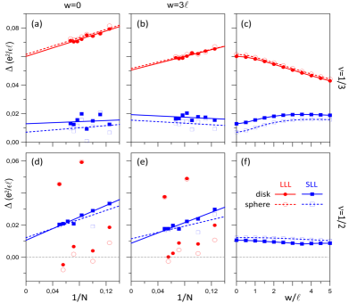
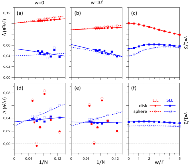
For comparison, in Figs. S4 and S5 we show the neutral and charge gaps obtained using the disk and spherical pseudopotentials for various widths at the Laughlin (extrapolated from ) and Pfaffian (extrapolated from ) fluxes in the SLL (see also Refs. Morf (1998); Wójs (2009)). For completeness, on the same plots, we have also included the corresponding LLL gaps. The ground state at the half-filled LLL is a compressible Fermi liquid state of composite fermions. Therefore, the gap in the LLL at the Pfaffian flux is irregular as a function of (the gap is only large when the flux and number of electrons are aliased with a Jain CF state), so we have not extrapolated it to the thermodynamic limit. We find that the gaps for the largest systems at and are a factor of 2-4 times larger than those for the -particle state. This indicates that the state is more fragile as compared to the experimentally observed and states.
III Comparison between some candidate and exact ground states in the second Landau level
The wave function for the parton state is most easily evaluated in the LLL in the first-quantized coordinate space (as opposed to the Hilbert space of Fock states). Therefore, to evaluate its second LL Coulomb energy, we use the effective interaction of Ref. Shi et al. (2008) to simulate the physics of the second LL in the LLL. This effective interaction has nearly the same Haldane pseudopotentials as that of the Coulomb interaction in the second LL. Including the contribution of the positively charged background, the per-particle density corrected Morf et al. (1986) energy of the parton state for the effective interaction for the system of particles is (the number in the parenthesis is the Monte Carlo uncertainty in the energy estimate) while the exact energy of the lowest-lying state is , both in Coulomb units of . The level of agreement (within ) between these two numbers is comparable with that of other trial states in the second LL Hutasoit et al. (2017); Balram et al. (2018b). The rest of the section is devoted to showing results for other candidate states and their comparison with the exact second LL Coulomb ground states.
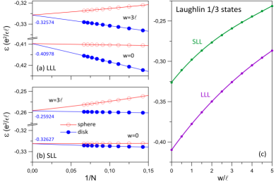
In Tables S1 and S2 we compare the overlap and energies of the Coulomb ground state in the two lowest Landau levels with the Laughlin and Pfaffian state respectively. For the largest system of electrons considered in this work, the energy of the Laughlin state differs from the exact second LL Coulomb energy by about . Similarly, the energy of the Pfaffian state of electrons is within of the exact second LL Coulomb ground state. These numbers are of the same order of magnitude as those of the parton state shown above. For completeness, in Figs. S6 and S7 we show the thermodynamic extrapolation and the extrapolated per-particle Coulomb energies of the Laughlin and Pfaffian states in the lowest and second Landau level obtained using the spherical and disk pseudopotentials at various finite widths.
| 6 | 15 | 0.52848 | -0.33306 | -0.32604 | 0.99645 | -0.41095 | -0.41075 | 0.58814 |
| 7 | 18 | 0.60705 | -0.33017 | -0.32611 | 0.99636 | -0.41082 | -0.41062 | 0.64941 |
| 8 | 21 | 0.57197 | -0.33071 | -0.32615 | 0.99540 | -0.41074 | -0.41052 | 0.62836 |
| 9 | 24 | 0.47941 | -0.33101 | -0.32617 | 0.99405 | -0.41068 | -0.41044 | 0.53871 |
| 10 | 27 | 0.54000 | -0.33043 | -0.32619 | 0.99295 | -0.41063 | -0.41038 | 0.60592 |
| 11 | 30 | 0.70303 | -0.32954 | -0.32620 | 0.99217 | -0.41058 | -0.41032 | 0.77057 |
| 12 | 33 | 0.50296 | -0.33039 | -0.32621 | 0.99092 | -0.41055 | -0.41028 | 0.57650 |
| 13 | 36 | 0.54445 | -0.33001 | -0.32622 | 0.98977 | -0.41052 | -0.41024 | 0.62202 |
| 14 | 39 | 0.57706 | -0.32984 | -0.32623 | 0.98871 | -0.41049 | -0.41020 | 0.66098 |
| 15 | 42 | 0.52978 | -0.32991 | -0.32623 | 0.98763 | -0.41047 | -0.41018 | 0.61475 |
| 6† | 9 | 0.81624 | -0.37528 | -0.37186 | 0.92280 | -0.46734 | -0.46275 | 0.53064 |
| 8† | 13 | 0.86739 | -0.37195 | -0.36966 | 0.92130 | -0.46175 | -0.45921 | 0.61067 |
| 10 | 17 | 0.83764 | -0.36968 | -0.36795 | 0.90537 | -0.46239 | -0.45931 | 0.55247 |
| 12† | 21 | 0.81939 | -0.36900 | -0.36678 | 0.65520 | -0.46651 | -0.45922 | 0.24462 |
| 14 † | 25 | 0.69345 | -0.36850 | -0.36621 | 0.72226 | -0.46367 | -0.45875 | 0.28091 |
| 16 | 29 | 0.77945 | -0.36767 | -0.36574 | 0.74587 | -0.46297 | -0.45854 | 0.33699 |
| 18 | 33 | 0.67656 | -0.36764 | -0.36536 | 0.63554 | -0.46400 | -0.45845 | 0.20746 |
| 20† | 37 | 0.67364 | -0.36723 | -0.36508 | 0.37029 | -0.46621 | -0.45834 | 0.08814 |
III.1 Updating results of Ref. Balram et al. (2018b)
The parton state, which is the predecessor of the parton state in the parton sequence, was posited as a candidate Balram et al. (2018b) to describe the experimentally observed FQHE FQHE Kumar et al. (2010). In Ref. Balram et al. (2018b), the parton state was compared against the exact SLL Coulomb ground state for only a single system of electrons at a flux of . At the time of publication, the next system size, that of electrons at a flux of , which has a Hilbert space dimension of , was not accessible to exact diagonalization. We have now been able to evaluate the exact SLL Coulomb ground state for this system size, which, to the best of our knowledge, is the largest system size for which the ground state of an FQHE Hamiltonian has been obtained. Improvements in the matrix times vector multiplication at each Lanczos iteration, which have made it possible to efficiently diagonalize such large matrices, have been described in Ref. Zuo et al. (2020).
The exact SLL Coulomb ground state for electrons at a flux of has that is consistent with realizing a uniform state. This system has a neutral gap of 0.0096 . In Fig. S9 we compare the pair-correlation function of the exact SLL Coulomb ground state with that of the parton state. The pair-correlation functions of both the parton state as well as the exact SLL Coulomb ground state show oscillations that decay at long distances, which is a typical feature of an incompressible state Kamilla et al. (1997); Balram et al. (2015c). Furthermore, of the exact SLL Coulomb ground state and the parton trial state match reasonably well with each other. Although the agreement is not conclusive, it is on par with that of other candidates in the SLL d’Ambrumenil and Reynolds (1988); Morf (1998); Scarola et al. (2002); Balram et al. (2013); Pakrouski et al. (2015); Hutasoit et al. (2017); Kuśmierz and Wójs (2018). For example, in Figs. S10 and S11 we show a comparison of the ’s of the Laughlin state Laughlin (1983) with that of the ground state and of the Pfaffian state Moore and Read (1991) with that of the ground state for the largest systems considered in this work. Thus, we conclude that the results for the electrons at flux provide further evidence for the feasibility of the parton state to describe the FQHE.
Including the contribution of the positively charged background, the per-particle density corrected Morf et al. (1986) energy of the parton state for the effective interaction that we use to simulate the physics of the SLL in the LLL for the system of particles at flux is while the exact energy of the ground state is , both in Coulomb units of . Again, the level of agreement (within ) between these two numbers is comparable with that of other candidate wave functions in the second LL Hutasoit et al. (2017); Balram et al. (2018b).
For completeness, we have also evaluated the exact LLL Coulomb ground state for the system at the flux of . The overlaps of the LLL and SLL Coulomb ground states is and their ’s are also very different from each other (see Fig. S9) which suggests that the ground state in the two LLs are quite different from each other for this system. We note that the system of electrons at a flux of aliases with the Jain CF state. As expected, we find excellent agreement between the ’s of the LLL Coulomb ground state and the Jain CF state for this system (see Fig. S9). Microscopically, the Jain CF states provide a very accurate representation of the exact LLL Coulomb ground states whereas the candidate states in the SLL provide only an approximate representation of the exact SLL Coulomb ground state. The neutral gap for the system of electrons at the flux in the LLL is 0.0487 (five times larger than the corresponding SLL neutral gap quoted above) indicating that the 2/5 Jain CF state is more robust than the parton state.