Fractional and scaled Brownian motion on the sphere: The effects of long-time correlations on navigation strategies
Abstract
We analyze fractional Brownian motion and scaled Brownian motion on the two-dimensional sphere . We find that the intrinsic long time correlations that characterize fractional Brownian motion collude with the specific dynamics (navigation strategies) carried out on the surface giving rise to rich transport properties. We focus our study on two classes of navigation strategies: one induced by a specific set of coordinates chosen for (we have chosen the spherical ones in the present analysis), for which we find that contrary to what occurs in the absence of such long-time correlations, non-equilibrium stationary distributions are attained. These results resemble those reported in confined flat spaces in one and two dimensions [Guggenberger et al. New J. Phys. 21 022002 (2019), Vojta et al. Phys. Rev. E 102, 032108 (2020)], however in the case analyzed here, there are no boundaries that affects the motion on the sphere. In contrast, when the navigation strategy chosen corresponds to a frame of reference moving with the particle (a Frenet-Serret reference system), then the equilibrium distribution on the sphere is recovered in the long-time limit. For both navigation strategies, the relaxation times towards the stationary distribution depend on the particular value of the Hurst parameter. We also show that on , scaled Brownian motion, distinguished by a time-dependent diffusion coefficient with a power-scaling, is independent of the navigation strategy finding a good agreement between the analytical calculations obtained from the solution of a time-dependent diffusion equation on , and the numerical results obtained from our numerical method to generate ensemble of trajectories.
The motion on non-Euclidean surfaces has gained great interest, particularly on the surface of a two-dimensional sphere , where the collusion between the intrinsic dynamics of the moving objects and the curved surface they are moving on, leads to singular and interesting effects Wisdom (2003); Avron and Kenneth (2006); Saporta Katz and Efrati (2019); Lin et al. (2020); Li et al. (2022). This growing interest is also encouraged by the fact that a variety of stochastic processes are equivalent to the diffusion of a tracer on the surface of a sphere, for instance, the tip of a unit vector that randomly rotates may describe the dynamics of a classical spin or the self-propulsion orientation of an active particle that moves with constant speed. Besides, the diffusive motion on curved surfaces is ubiquitous in different biological processes such as the motion of proteins or phospholipids (PIP2 Fujiwara et al. (2002); Metzler et al. (2016)) on the cell membrane, which is crucial for cell signaling Haastert and Devrotes (2004); Ma et al. (2004); van Meer et al. (2008); Meyers et al. (2006); Hancock (2010); cell migration confined to curved surfaces Werner et al. (2017); Bade et al. (2018); Pieuchot et al. (2018); Lin et al. (2020); or the pattern formation of epithelial tissue Xi et al. (2017); Yu et al. (2021); Happel et al. (2022). Additionally, the motion of active particles diffusing on the sphere has been analyzed at the single particle and collective level Castro-Villarreal and Sevilla (2018); Praetorius et al. (2018); Sknepnek and Henkes (2015); Apaza and Sandoval (2017); Shankar et al. (2017); Ai et al. (2020); Henkes et al. (2018); Gnidovec and Čopar (2020); Hsu et al. (2022); Piro et al. (2022).
An experimental analysis of the effects on particle diffusion due to the curvature of the underlying surface, has been carried out on polystyrene nanoparticles diffusing on the interface of a silicone-oil droplet immersed in water Zhong et al. (2017), while theoretical analysis of different effects—curvature gradient, external forces, many-body interactions—on the diffusion of particles confined to surfaces have been analyzed lately Ramírez-Garza et al. (2021); Valdés-Gómez and Sevilla (2021); Montañez-Rodríguez et al. (2021); Ledesma-Durán et al. (2021).
Despite of the important advances just mentioned, to our knowledge, the effects of long-time correlations on the motion of a particle moving on the surface of a compact manifold has not been studied, yet being of relevance since such processes model diverse mechanisms that lead to persistent (and antipersistent as well) motion on curved surfaces. In this article we address these aspects and fill this gap by analyzing the effects of long-time correlated diffusion on the one hand, and the effects of a time-dependent diffusion coefficient on the other, of a tracer particle moving on the surface of the two-dimensional sphere, . These two processes may arise from the complex interactions between the diffusing particle and the variety of components that lie on the sphere surface, such as in the cell membrane. A relevant aspect of our study is the elucidation of the nontrivial concomitant effects caused by the long-time correlations of the diffusive process of a tracer particle on a compact manifold, in this case, and distinct navigation strategies.
The observation of long-time correlated Brownian processes, i.e., those for which the autocorrelation function of the particles position decays slowly with time in the form of a power law time-dependence, has been recognized to be ubiquitous in nature. This kind of correlations generally occurs in Brownian-like motion of particles in crowded environments, where the complex coupling of the Brownian particle with the environment leads to long-lasting correlations. This has been pointed out since the classical work of Alder and Wainwright Alder and Wainwright (1967, 1970) and of Widom Widom (1971), where it is shown that the coupling of a hard-core Brownian particle moving in an incompressible viscous fluid, leads to a velocity autocorrelation function that decays asymptotically as , instead of the exponentially fast relaxation, thus pointing out the role of the environment through hydrodynamic interactions Pomeau and Résibois (1975). Following this rationale, a modification of the Langevin equation is carried out to take into consideration the fluid inertia Hinch (1975) and recovering the algebraic decay of the velocity correlation function. Algebraic decay was subsequently observed in the experiments of Paul and Pusey Paul and Pusey (1981) and Clercx and Schram Clercx and Schram (1992).
The overdamped motion of a particle moving in complex crowded environments, can exhibit a variety of behaviors. The most interesting being perhaps, anomalous diffusion, which is characterized by the power-law time scaling found for the time dependence of the mean squared displacement, , with , but . It is widely accepted that such scaling is ubiquitous and originates from the long-time correlations of motion, which in turn, depend on the particular coupling between the environment and the particle Höfling and Franosch (2013). For instance, subdiffusion () of submicron tracers was observed experimentally in the the motion of proteins embedded in the membranes of living cells Weiss et al. (2003); Weigel et al. (2011); Manzo et al. (2015); He et al. (2016); also in the cytoplasm of biological cells Weiss et al. (2004); Caspi et al. (2000); Seisenberger et al. (2001); Golding and Cox (2006); Jeon et al. (2011); Tabei et al. (2013); and in crowded liquids Banks and Fradin (2005); Szymanski and Weiss (2009); Jeon et al. (2013).
Different mathematical frameworks (models) have been ingeniously devised to describe anomalous diffusion Metzler et al. (2014), and two of them stand out as they take into consideration the memory effects that arise, in most of the cases, from a reduced description focusing on the dynamics of the tracer particle dynamics from the rest of the elements that influence its motion. One corresponds to the generalized master equation *[Hola][ThereadershouldfocusonsectIV.]KenkreChapter1977 (or Continuous-Time Random Walks Kenkre et al. (1973)), which for power-law time memories leads to the fractional diffusion equations of Metzler and Klafter and other authors Wyss (1986); Metzler and Klafter (2000), that incorporate the fractional derivative, where the order of integrals and derivatives are generalized to fractional order Podlubny and (Eds.); TARASOV (2013); West (2014); Sandev and Tomovski (2019). The other model that considers memory effects goes back to the seminal work of Kubo, and nowadays is referred as the generalized Langevin equation Kubo (1966). This takes into account the retarded effect of the dissipative force and becomes the fractional Langevin equation when the memory is chosen in the class of memory function with power-law time dependence Kobelev and Romanov (2000); Lutz (2001); Burov and Barkai (2008). This theoretical framework has found diverse applications, particularly in the analysis of the diffusion of Brownian motion in viscoelastic fluids Rodriguez and Salinas-Rodriguez (1988), where the hydrodynamic interaction, as noticed by Boussinesq (see Ref. Makris (2021) for a historical recount) plays an important role in the dynamics.
In this work we resort to fractional Brownian motion (fBm) as a simple model of long-time correlated motion which was introduced by Mandelbrot and van Ness (and based in the previous work by Kolgomorov, Hurst, Hunt, Lamperti and Yaglom), to model natural time series that exhibits extremely long interdependence Mandelbrot and Van Ness (1968). This stochastic process has gained interest in different contexts, particularly regarding anomalous diffusion, due to its simple, but non-trivial, intrinsic characteristics: being Gaussian, self-similar and with stationary increments Metzler et al. (2014); Sokolov (2012); Biagini et al. (2008). Although the “fractional” character in this case is different from the one of fractional derivatives, a connection with the overdamped limit of a fractional Langevin equation has been conveyed in Ref. Sokolov (2012).
In addition, we also consider the case of scaled Brownian motion (sBm), which defines a Gaussian process characterized by the time-dependent diffusion coefficient . In unbounded Euclidean space, sBm is defined by the solution of the diffusion equation with time-dependent diffusion coefficient and leads to the power-law scaling of the mean squared displacement Jeon et al. (2014); Thiel and Sokolov (2014), although no long-time correlated motion is involved. In here we use the same symbols and as in fBm since they have the same physical units, however, they have different physical meaning as they characterize two different stochastic processes; in Ref. Jeon et al. (2014), it is shown that under confinement, the stochastic process given by sBm is fundamentally distinct from fBm. We show in this paper that this is also the case when the motion occurs freely on .
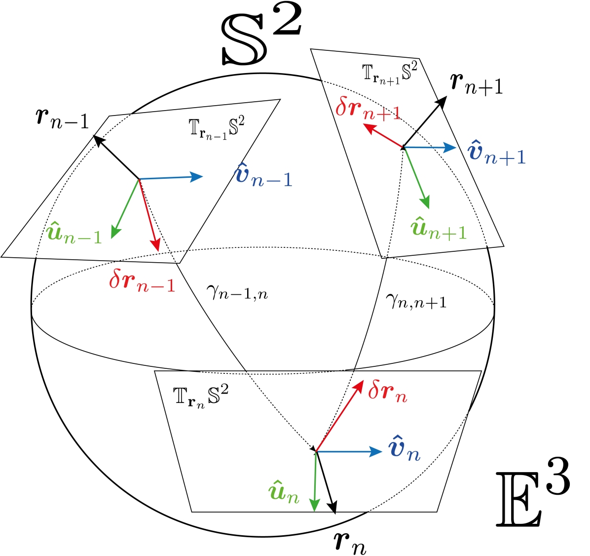
We analyze a statistical ensemble of discretized trajectories generated by extending the method presented in Ref. Valdés-Gómez and Sevilla (2021). Such an extension takes into account either the long-time correlations of the motion, or the time-dependence of the diffusion coefficient of a non-stationary diffusion process. Briefly, an element of the ensemble is generated by recursively updating the particle position, initiating at on at time , such that in a time interval , the particle position at the -th step is obtained from the previous one as
| (1) |
where lies on the tangent plane centered at on the sphere; is an orthonormal basis of (see left panel in Fig. 1); and , are two statistically independent increments obtained from the underlying stochastic process considered. The updating rule (1) considers the factor
| (2) |
which rescales such that is projected along the corresponding geodesic with the correct arc length. The operator being , with the sphere radius (unit vectors are defined as ). The tangent plane and the four referred vectors are displayed in the left panel of Fig. 1, for three consecutive iterations. The positions , orthogonal to , are depicted in black, the displacements on the plane are depicted in red, while the basis vectors and are depicted in green and blue, respectively.
The long-time correlated motion considered for our analysis is carried out by mapping to the sphere surface (through the use of Eq. ), two statistically independent fBm processes. In the case when the stochastic motion is characterized by a time-dependent diffusion coefficient, we use the so-called scaled Brownian motion (sBm) for which the diffusion coefficient scales with time as with .
Fractional Brownian motion on .-
To generate long-time correlated trajectories we consider two statistically independent fBm processes, and , characterized by Hurst exponents , respectively. These are Gaussian stochastic processes with and autocorrelation function
| (3) |
where (with units of [length][time]-2H) measures its amplitude. Eq. (3) reduces to the auto-correlation of the Wiener process when and gives at equal times for all in . The fBm process is also defined as the integral of fractional Gaussian noise , as , is a stationary stochastic process with autocorrelation function Qian (2003), from which is recognized a time-dependent diffusion coefficient .
We are interested in the case for which , however an extension to the anisotropic case is straightforward. The increments of the fBms during the time interval , , and (corresponding to the increments and respectively), are stationary, long-time correlated, and not independent if . In the case they are negatively correlated, while they are positively correlated if Biagini et al. (2008). In this case the increment is given by , with an orthonormal vector basis for .
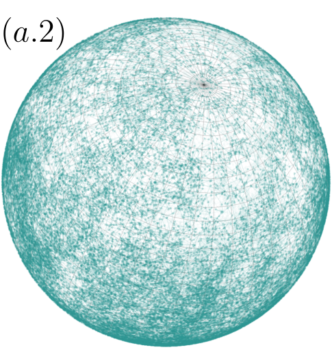
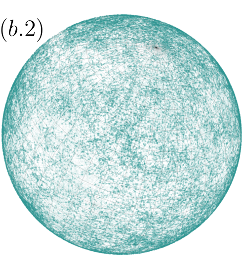
We found that the long-time correlations of fBm () collude with the specific implementation of the updating rule (1) through the choice of the orthonormal basis , which defines a kind of navigation strategy that drives the particle motion to give rise to a rich variety of statistical patterns of motion on the sphere. On the contrary, uncorrelated motion (as is the standard Brownian motion, ) is insensitive to the choice of such strategies [see (a.2) and (b.2) for a qualitative comparison in the right panel in Fig. 1].
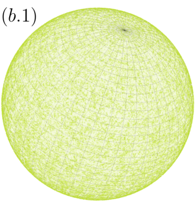
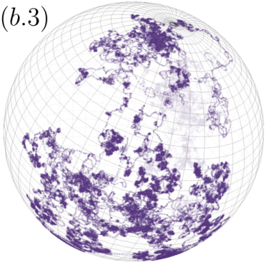
We consider for our analysis two contrasting physically-motivated navigation strategies, one is observed in many biological organisms which may have a distinct body axis (head-tail axis) defining a preferred direction of motion sometimes referred as heading. In such a case the particle heading , together with the normal vector , form the orthonormal basis for the updating rule (1) that carry the long-term correlated motion. Notice that with (the binormal vector), these three vectors form the well-known Frenet-Serret system. Three sample trajectories are shown: (b.1), (b.2) and (b.3), in the second column of the right panel of Fig. 1, for highly anticorrelated motion, (b.1), uncorrelated motion, (b.2), and highly correlated motion, (b.3).
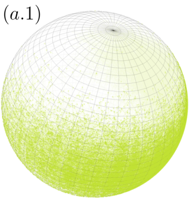
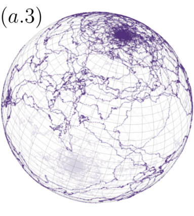
The other navigation strategy corresponds to the case for which the orthonormal basis for the updating rule, , forms a kind of “laboratory reference frame”, which for our analysis is chosen to be the one induced by the spherical coordinates of , and consequently attached to each point of the sphere surface, namely, , oriented along the sphere meridians, and orthogonally oriented along the parallels (see left panel in Fig. 1). As a consequence, the long-time correlated trajectories describe a distinct pattern as is shown by the trajectories shown in the right panel of Fig. 1 for (a.1) and (a.3). Self-confinement is observed for , each particle excursion is limited to a sector of the sphere around well-defined time-average values , that depend on . For , particles concentrate forming an island around (equator) with randomly chosen; while for distinctively, the particles concentrate their excursions around the poles, i.e. , wandering between them as is shown in Fig. 1(a.3). For this navigation strategy, ensemble averages strikingly differs from time averages giving rise to weak ergodicity breaking Thiel and Sokolov (2014), especially for , for which single trajectories get trapped diffusing around a randomly chosen sector of the sphere, thus, the time average using a single long trajectory will differ from the ensemble average which samples uniformly those sectors; the equivalence between ensemble averages and time averages is recovered for [see a trajectory generated in Fig. 1(a.2)].
Scaled Brownian motion on .-
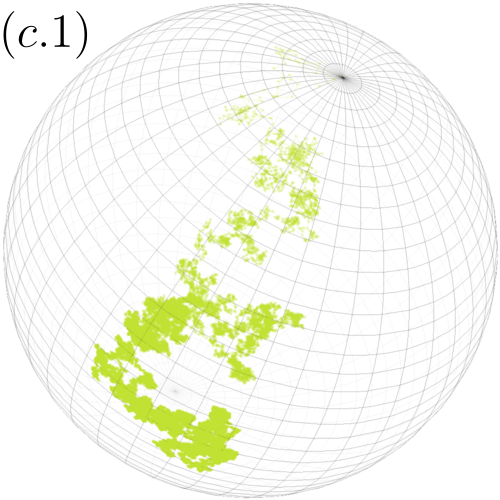
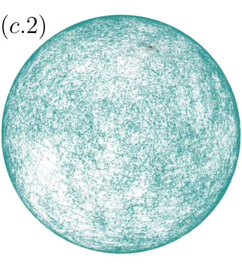
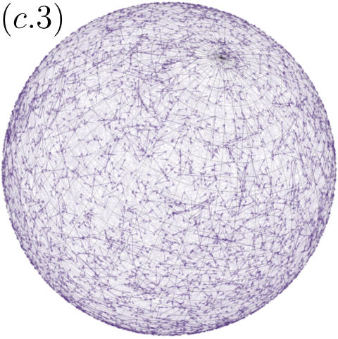
The other pattern of stochastic motion we address in this paper refers to sBm. The updating rule (1) in this case considers two independent Gaussian processes and , with statistically independent increments , and , for the time increment , ; , are two independent Wiener processes of vanishing mean and unitary variance; and being the total time elapsed up to step . Scaled Brownian motion is highly non-stationary due to the time-dependence of the diffusion coefficient, a feature that is implemented by considering , where we have assumed homogeneous time increments , and the pair of orthonormal vectors is an arbitrary vector basis for . It is the statistical independence among the increments what guaranties that the updating rule is independent of the basis choice, as occurs for uncorrelated standard Brownian motion (or fBm with ). Three sBm trajectories are shown in the third column of the right panel of Fig. 1 for (c.1), (c.2) and (c.3), which are contrasted with those for the two navigation strategies considered for the fractional Brownian motion case (trajectories in the first and second columns in the same figure).
The corresponding modification of the Euclidean Fokker-Planck equation that considers that sBm occurs on is
| (4) |
where denotes the particle’s position in spherical coordinates, being the radius of . The solution of (4) is given by
| (5) |
the coefficients are determined from the initial distribution, and are the standard spherical harmonics. If the initial condition corresponds to a localized distribution at the north pole we get
| (6) |
with the Legendre polynomials. The absence of in (6) implies the azimuthal symmetry of the process, which leads to the moments of the polar angle , given by
| (7) |
where . It is clear from (6) that for each , the marginal stationary distribution of the polar angle, , is attained in the long-time regime, indicating the uniform distribution of the particle positions on .
In addition the auto-correlation function of the particle positions can be computed straightforwardly and is given by
| (8) |
Notice that the time dependence of the quantities computed from Eq. (4), namely and , become -invariant under the time-scaling transformation . Such transformation makes Eq. (4) -invariant leading to dynamical scaling as can be checked straightforwardly.
Frequency distribution of the polar angle for fBm: The role of the navigation strategy.-
We present an statistical analysis of a set of ensembles of trajectories generated with the method described in the previous paragraphs: Two subsets corresponding to fBm, one for each of the navigation strategies considered; and one subset corresponding to sBm. In the case of fBm each ensemble consisted of 5 trajectories for each of the nine values of the considered, namely for which we have set in arbitrary units. For sBm the absence of long-time correlations allow to consider ensembles of 1.2 trajectories.
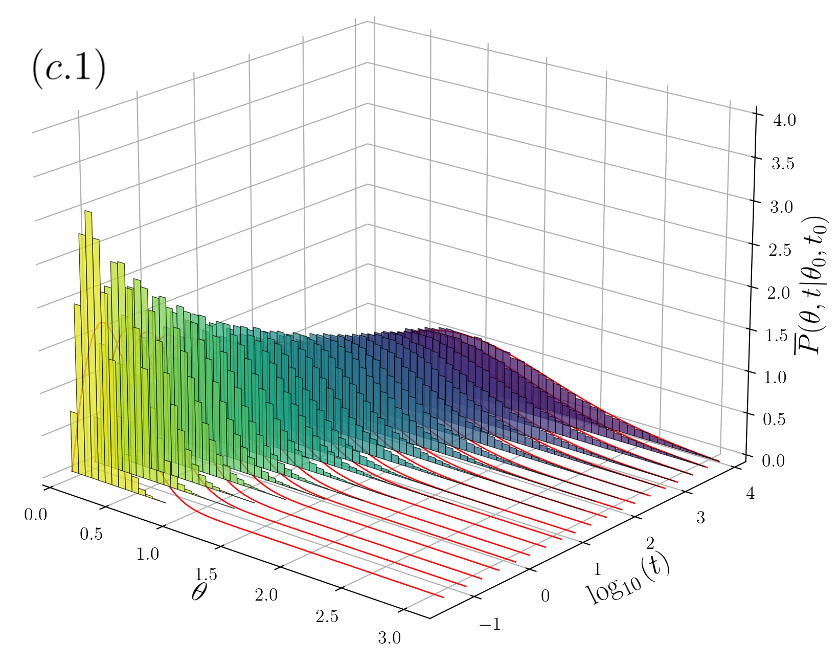
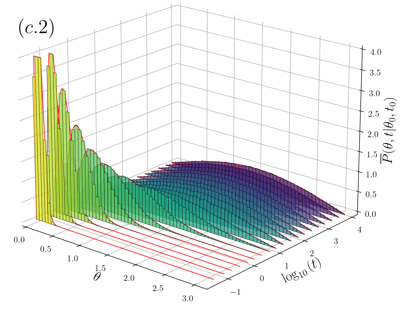
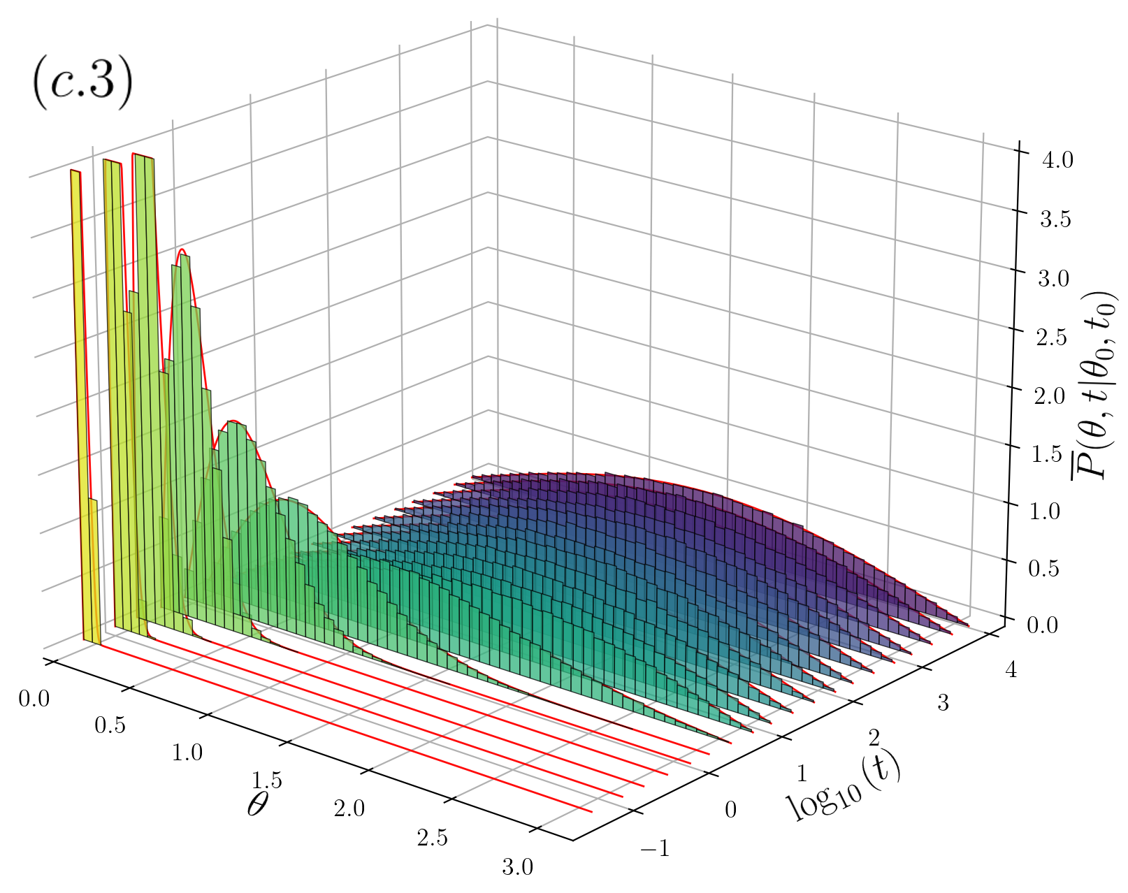
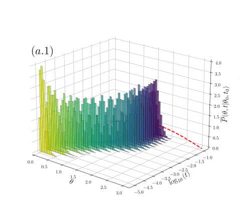
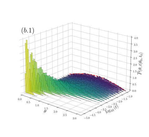
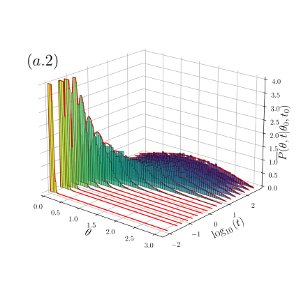
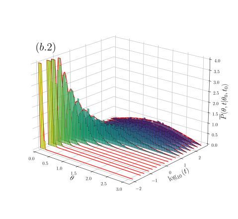
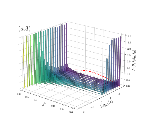
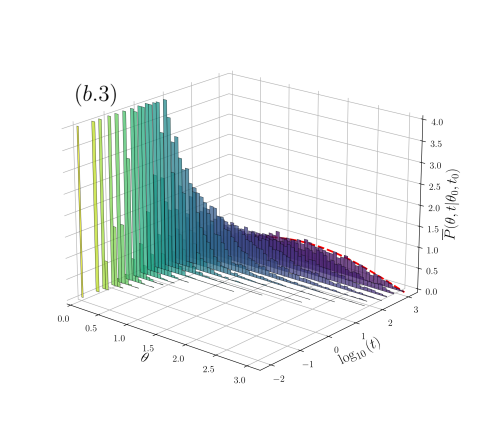
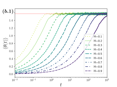
Each ensemble of trajectories was generated with fixed initial position at the sphere’s north pole , this choice allows us to assume an azimuthal symmetry in the ensemble average and therefore to focus on the frequency distribution of the polar angle only. From each ensemble, the frequency histograms of the polar angle , with at , is computed at each time step giving rise to the time evolution shown in Figs. 2 and 3; in Fig. 2 we show the case for fractional Brownian motion, for which long-time correlations make manifest the role of the navigation strategy through the basis system chosen at each . In Fig. 3 we show the corresponding histograms for the case of sBm.
For the Frenet-Serret navigation strategy (second column of Fig. 2), the system attains the stationary distribution for each , this is shown in the evolution of the frequency histograms in the plots of the second column of Fig. 2 for (b.1), 0.5 (b.2) and 0.9 (b.3) respectively ( is depicted by the dashed-red line). Notice that the relaxation times towards depend on , being shorter the smaller is [compare the time scales considered from (b.1) to (b.3) histograms in the second column of Fig. 2]. In contrast, for the navigation strategy , the system attains a non-equilibrium stationary state (except for the uncorrelated case , for which the attained stationary state is independent of the navigation strategy and coincides with shown in the histograms of (a.2) of Fig. 2). For anti-correlated motion () the frequency histograms settle into a unimodal distribution, highly peaked around the equator line () the smaller the value of [see histograms in (a.1) of Fig. 2 for ], the distribution transforms continuously into as (a.2). For correlated motion () the stationary distribution settles into a bimodal distribution with modes at the sphere poles [see histograms in (a.3) of Fig. 2 for ], such stationary distribution is determined by the specific basis chosen only, and does not depend on the initial distribution. Thus, the poles can be interpreted as being repulsive if , and being attractive if . These non-equilibrium stationary distributions, when , are attained independently of the initial distribution.
Analogous effects to the ones observed with the basis induced by the spherical coordinates have been observed in confined fBm, specifically as result of the interplay of long-time correlations and hard-walls boundaries Wada and Vojta (2018); Guggenberger et al. (2019); Vojta et al. (2020), where depleted regions for the probability distribution of the particle positions are observed near the boundaries for anticorrelated motion (), while accreted regions near the boundaries are observed for .
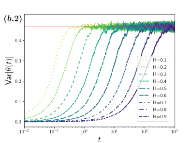
In Fig. 3 shows for sBm. is attained for all and the cases (c.1), (c.2) and (c.3) are shown. Excellent agreement is observed except for the short-time regime of and 0.2, where there is some discrepancy due to numerical stability.
I Comparative analysis of the cases considered.-
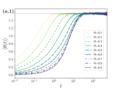
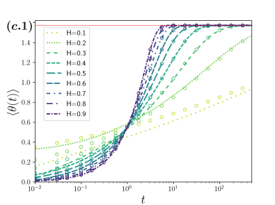
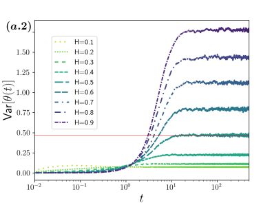
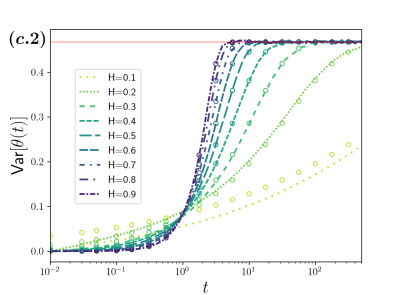
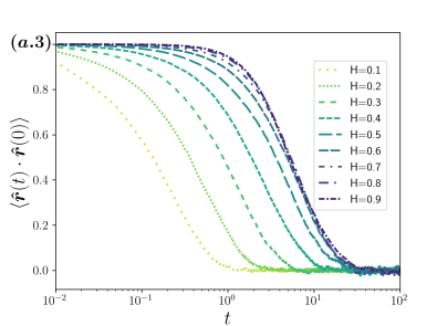
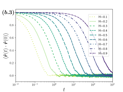
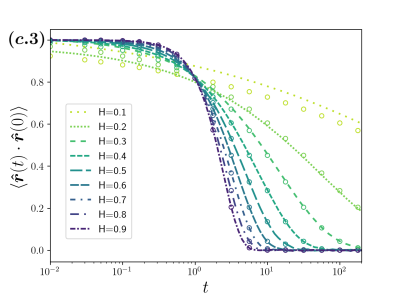
The qualitatively different behavior among the three cases considered is apparent from the analysis of the time dependence of three relevant statistical quantities of the distribution of the polar angle, namely: The mean , the variance , and the position autocorrelation function , all of them shown in Fig. 4 and identified with the numerals 1, 2 and 3 correspondingly; the column (a) corresponds to the case of fBm with navigation strategy , the (b) one for fBm with and the column (c) for sBm, which is independent of the navigation strategy. For each case considered we have , with xBm either fBm or sBm as appropriate.
Notorious differences caused by the navigation strategy in the time evolution of the quantities considered can be observed for fBm. On the one hand, in the case of the basis , separates two qualitatively distinct behaviors. For the position autocorrelation decays faster than for the case the smaller is (see (a.3) in Fig. 4), as consequence, the mean approaches the value , also faster the smaller is (see (a.1) in Fig. 4)]. For the correlations decay slower than for , however, the time dependence in this case is similar. In each case the distributions are symmetric around the equator thus saturates at . The departure from the uniform distribution on is evidenced by the time dependence of the variance [(a.2) in Fig. 4], which clearly indicates a smaller dispersion around the mean for (the distributions are more peaked around the mean with kurtosis for , for , for and for , with respect to the uniform distribution, , whose kurtosis has the exact value ). Larger dispersion is observed for due to the bimodality of the distribution of (the variance of the distribution highly peaked at the poles, notice that the distribution has variance which serves as an upper bound for the values presented in (a.2) of Fig. 4).
When the basis used is the position autocorrelation decays with a relaxation time that increases monotonically with as is shown in (b.3) of Fig. 4. Similarly, the mean (b.1) and variance (b.2) saturate to the values of at a pace that depends monotonically on , the smaller the the faster reaches the values corresponding to .
It is clear from these results that for a basis pinned on the manifold induced by a set of local coordinates, as for the spherical coordinates analyzed here, anti-correlated motion () makes the sphere poles to be seldom visited (the regions around the poles are diluted in the ensemble) in contrast, for correlated motion (), the region around the sphere poles are frequently visited. It is only for (non-correlated motion) from which the uniform stationary distribution is attained, for which each location on the sphere should be visited as frequently as any other independently of the initial distribution. We thus conclude that long-correlated motion breaks the spherical symmetry of the stationary state for locally-coordinates induced basis . In constrast, fully spherical symmetry of the stationary state is attained for all values of for a basis unpinned from the sphere local coordinates, as shown here for the Frenet-Serret system that serves as a body-reference system.
Finally, we contrast the results obtained for sBm (column (c) in Fig. 4) with those presented for fBm. Since long-time correlations do not collude with navigation strategy in the sBm case, is attained in the long-time regime for all . The position autocorrelations decay faster the larger is, which is a consequence of the fact that the distribution of the polar angle relaxes faster with in contrast with fBm case. The time dependence of the mean [4 (c.1)], variance [4 (c.2)] and position autocorrelation function [4 (c.3)] are shown in the column (c) in Fig. 4, where calculations from the ensemble (lines) are compared with the analytical expression given by the the stretched exponential in Eq. (8) (open dots). The discrepancy observed for the smaller values of is mainly due to the combined effects of the large fluctuations induced by the time dependence of the diffusion coefficient in the short-time regime and size of our ensemble of trajectories. We want to comment in passing that due to the -invariance of sBm under the scaling transformation , the curves presented in Fig. 4 will overlap on top of each other if plotted as function of instead of .
Concluding remarks.-
We studied fractional Brownian motion as a model of long-time correlated motion of a particle that randomly swims on the surface of a sphere. We elucidated the deep connection of this process with different navigation strategies defined by a particular basis for the tangent planes to that specifies the updating rule of the algorithm used to analyze random motion on the sphere. In the case of uncorrelated motion (for which fBm with is a particular case), the dynamics is independent of the navigation strategy coinciding with standard Brownian motion on the sphere. Furthermore, we formulated the updating rules in the algorithm used (Eqs. (1)-(2)) to analyze the diffusion processes characterized by a time-dependent diffusion coefficient , and focused in scaled Brownian motion for which .
We found that for the navigation strategy induced by the spherical coordinates, two qualitatively distinct trajectory patterns are observed depending on whether or which lead to non-equilibrium stationary states. The equilibrium stationary distribution is recovered for the navigation strategy induced by the Frenet-Serret system which unpins the long-time correlated motion from a basis that depends on the local coordinates. These observations allow to conclude that long-time correlated motion collude with the class of navigation strategies that locally depend on the coordinates chosen, leading to “nonequilibrium steady states” breaking down equilibrium dynamics, this last one is restored for the class of coordinates-independent navigation strategies (Brownian motion and sBm).
The similarity of the effects reported here for the coordinates-dependent navigation strategy in fBm (the sphere poles are seldom visited for while frequently visited for ), with those occurring in confined fBm in Euclidean space (depletion of the position distribution around reflecting walls for and accumulation for ) reported in Ref. Vojta et al. (2020) are remarkable, and compels to conjecture that such similarity finds its origin in the coordinates-dependent navigation strategy chosen. It is plausible that if the body-reference system is employed in the dynamics in Euclidean space, instead of a fixed local space basis, it will restore a dynamics that leads to the uniform distribution in the long-time regime. Research in this direction has been started and the corresponding results will be published elsewhere.
To conclude we can classify the navigation strategies into two main classes: Those that are pinned to the manifold by a particular choice of coordinates basis for each tangent plane ; and those that are fixed at the body-reference system. Both situations are plausible to occur in real systems. For instance, the lateral movement of organic molecules on the cell membrane, are subject to a variety of effects induced by the surface (many lipids distributed on the membrane serve as obstacles) on which the molecules move (this would lead to a navigation strategy pinned to the manifold). This is the case for the lateral movement of signaling phosphatidylinositol lipids (PIP2, PIP3, PIP McLaughlin et al. (2002); Beard and Oian (2008); Hancock (2010)) on the cell membrane. Diffusion of these molecules is affected by the interaction with the cell membrane lipids and other of its components Philip L. (2005); Brogh et al. (2005); Fujiwara et al. (2002); Blind et al. (2014); Buckles et al. (2017), thus any mobility correlations arise from the distribution of obstacles in the cell membrane surface, and therefore can be modeled by use of a reference frame fixed in the cell membrane. These same effects make water molecules to subdiffuse on the cell membrane Yamamoto et al. (2014). With the recent advances designing cell membranes coated particles Spanjers and Städler (2020), the diffusion of proteins on such surfaces can be modified either by the shape of the coated particle or by the properties of the coating membrane. In the same trend and with the aim to overcome the obstacles faced by traditional synthetic micromotors, active (or self-propelling) micromotors have been cell membrane-functionalized to enhance mobility due to motility induced persistence Esteban-Fernández de Ávila et al. (2018); Wu et al. (2020); Zhang et al. (2022) these are able to navigate tissue, subject to an “internal” navigation scheme (navigation strategy that depends on the body-reference) that arise from the self-propulsion mechanisms.The effects of fBm on the self-propulsion dynamics of active particles moving in two-dimensional space have been analyzed in Ref. Gomez-Solano and Sevilla (2020).
Finally, single-tracking methods have provided evidence that motion in crowded environments, particularly molecular motion in the cell membrane (transmembrane motion), is not as simple as Brownian motion Ritchie et al. (2005); Höfling and Franosch (2013); Metzler et al. (2016). This has led to the formulation of a variety of diffusion models to capture the anomalous diffusion behavior of these elements. Those based on fractional Brownian motion have shed light in the understanding of anomalous diffusion in numerous biophysical systems Benelli and Weiss (2021); Ernst et al. (2012); Sadoon and Wang (2018); Sabri et al. (2020); Speckner and Weiss (2021).
In this paper we have highlighted the non-trivial effects of the interplay between the reference frame, that describe the motion of particles moving on the surface of the sphere, and the long correlations of the motion. The analysis presented has potential applications to biophysical systems, particularly in the analysis of the diffusion of molecules in biological membranes, where the motion, besides being stochastic, is in many cases long-time correlated.
Acknowledgements.
This work was supported by UNAM-PAPIIT IN112623.References
- Wisdom (2003) J. Wisdom, Science 299, 1865 (2003),
- Avron and Kenneth (2006) J. E. Avron and O. Kenneth, New Journal of Physics 8, 68 (2006),
- Saporta Katz and Efrati (2019) O. Saporta Katz and E. Efrati, Phys. Rev. Lett. 122, 024102 (2019),
- Lin et al. (2020) S.-Z. Lin, Y. Li, J. Ji, B. Li, and X.-Q. Feng, Soft Matter 16, 2941 (2020),
- Li et al. (2022) S. Li, T. Wang, V. H. Kojouharov, J. McInerney, E. Aydin, Y. Ozkan-Aydin, D. I. Goldman, and D. Z. Rocklin, Proceedings of the National Academy of Sciences 119, e2200924119 (2022),
- Fujiwara et al. (2002) T. Fujiwara, K. Ritchie, H. Murakoshi, K. Jacobson, and A. Kusumi, Journal of Cell Biology 157, 1071 (2002), ISSN 0021-9525,
- Metzler et al. (2016) R. Metzler, J.-H. Jeon, and A. Cherstvy, Biochimica et Biophysica Acta (BBA) - Biomembranes 1858, 2451 (2016), ISSN 0005-2736, biosimulations of lipid membranes coupled to experiments,
- Haastert and Devrotes (2004) P. J. M. Van Haastert and P. N. Devrotes, Nat. Rev. Mol. Cell. Biol. 5, 626 (2004).
- Ma et al. (2004) L. Ma, C. Janetopoulos, L. Yang, P. N. Devrotes, and P. A. Iglesias, Biophysical Journal 87, 3764 (2004).
- van Meer et al. (2008) G. van Meer, D. R. Voelker, and G. W. Feigenson, Nat. Rev. Mol. Cell. Biol. 9, 112 (2008).
- Meyers et al. (2006) J. Meyers, J. Craig, and D. J. Odde, Current Biology 16, 1685 (2006).
- Hancock (2010) J. T. Hancock, Cell Signalling (Oxford University Press Inc., New York, 2010).
- Werner et al. (2017) M. Werner, S. B. G. Blanquer, S. P. Haimi, G. Korus, J. W. C. Dunlop, G. N. Duda, D. W. Grijpma, and A. Petersen, Advanced Science 4, 1600347 (2017),
- Bade et al. (2018) N. D. Bade, T. Xu, R. D. Kamien, R. K. Assoian, and K. J. Stebe, Biophysical Journal 114, 1467 (2018), ISSN 0006-3495,
- Pieuchot et al. (2018) L. Pieuchot, J. Marteau, A. Guignandon, T. Dos Santos, I. Brigaud, P.-F. Chauvy, T. Cloatre, A. Ponche, T. Petithory, P. Rougerie, et al., Nature Communications 9, 3995 (2018), ISSN 2041-1723,
- Xi et al. (2017) W. Xi, S. Sonam, T. Beng Saw, B. Ladoux, and C. Teck Lim, Nature Communications 8, 1517 (2017), ISSN 2041-1723,
- Yu et al. (2021) S.-M. Yu, B. Li, F. Amblard, S. Granick, and Y.-K. Cho, Biomaterials 265, 120420 (2021), ISSN 0142-9612,
- Happel et al. (2022) L. Happel, D. Wenzel, and A. Voigt, Effects of local curvature on epithelia tissue – coordinated rotational movement and other spatiotemporal arrangements (2022),
- Castro-Villarreal and Sevilla (2018) P. Castro-Villarreal and F. J. Sevilla, Phys. Rev. E 97, 052605 (2018),
- Praetorius et al. (2018) S. Praetorius, A. Voigt, R. Wittkowski, and H. Löwen, Phys. Rev. E 97, 052615 (2018),
- Sknepnek and Henkes (2015) R. Sknepnek and S. Henkes, Phys. Rev. E 91, 022306 (2015),
- Apaza and Sandoval (2017) L. Apaza and M. Sandoval, Phys. Rev. E 96, 022606 (2017),
- Shankar et al. (2017) S. Shankar, M. J. Bowick, and M. C. Marchetti, Phys. Rev. X 7, 031039 (2017),
- Ai et al. (2020) B.-q. Ai, B.-y. Zhou, and X.-m. Zhang, Soft Matter 16, 4710 (2020),
- Henkes et al. (2018) S. Henkes, M. C. Marchetti, and R. Sknepnek, Phys. Rev. E 97, 042605 (2018),
- Gnidovec and Čopar (2020) A. c. v. Gnidovec and S. Čopar, Phys. Rev. B 102, 075416 (2020),
- Hsu et al. (2022) C.-P. Hsu, A. Sciortino, Y. A. de la Trobe, and A. R. Bausch, Nature Communications 13, 2579 (2022), ISSN 2041-1723,
- Piro et al. (2022) L. Piro, B. Mahault, and R. Golestanian, New Journal of Physics 24, 093037 (2022),
- Zhong et al. (2017) Y. Zhong, L. Zhao, P. M. Tyrlik, and G. Wang, The Journal of Physical Chemistry C 121, 8023 (2017),
- Ramírez-Garza et al. (2021) O. A. Ramírez-Garza, J. M. Méndez-Alcaraz, and P. González-Mozuelos, Phys. Chem. Chem. Phys. 23, 8661 (2021),
- Valdés-Gómez and Sevilla (2021) A. Valdés-Gómez and F. J. Sevilla, Journal of Statistical Mechanics: Theory and Experiment 2021, 083210 (2021),
- Montañez-Rodríguez et al. (2021) A. Montañez-Rodríguez, C. Quintana, and P. González-Mozuelos, Physica A: Statistical Mechanics and its Applications 574, 126012 (2021), ISSN 0378-4371,
- Ledesma-Durán et al. (2021) A. Ledesma-Durán, J. Munguía-Valadez, J. A. Moreno-Razo, S. I. Hernández, and I. Santamaría-Holek, Front. Phys. 9, 634792 (2021), ISSN 2296-424X,
- Alder and Wainwright (1967) B. J. Alder and T. E. Wainwright, Phys. Rev. Lett. 18, 988 (1967),
- Alder and Wainwright (1970) B. J. Alder and T. E. Wainwright, Phys. Rev. A 1, 18 (1970),
- Widom (1971) A. Widom, Phys. Rev. A 3, 1394 (1971),
- Pomeau and Résibois (1975) Y. Pomeau and P. Résibois, Physics Reports 19, 63 (1975), ISSN 0370-1573,
- Hinch (1975) E. J. Hinch, Journal of Fluid Mechanics 72, 499–511 (1975).
- Paul and Pusey (1981) G. L. Paul and P. N. Pusey, Journal of Physics A: Mathematical and General 14, 3301 (1981),
- Clercx and Schram (1992) H. J. H. Clercx and P. P. J. M. Schram, Phys. Rev. A 46, 1942 (1992),
- Höfling and Franosch (2013) F. Höfling and T. Franosch, Reports on Progress in Physics 76, 046602 (2013),
- Weiss et al. (2003) M. Weiss, H. Hashimoto, and T. Nilsson, Biophysical Journal 84, 4043 (2003), ISSN 0006-3495,
- Weigel et al. (2011) A. V. Weigel, B. Simon, M. M. Tamkun, and D. Krapf, Proceedings of the National Academy of Sciences 108, 6438 (2011),
- Manzo et al. (2015) C. Manzo, J. A. Torreno-Pina, P. Massignan, G. J. Lapeyre, M. Lewenstein, and M. F. Garcia Parajo, Phys. Rev. X 5, 011021 (2015),
- He et al. (2016) W. He, H. Song, Y. Su, L. Geng, B. J. Ackerson, H. B. Peng, and P. Tong, Nature Communications 7, 11701 (2016), ISSN 2041-1723,
- Weiss et al. (2004) M. Weiss, M. Elsner, F. Kartberg, and T. Nilsson, Biophysical Journal 87, 3518 (2004), ISSN 0006-3495,
- Caspi et al. (2000) A. Caspi, R. Granek, and M. Elbaum, Phys. Rev. Lett. 85, 5655 (2000),
- Seisenberger et al. (2001) G. Seisenberger, M. U. Ried, T. Endreß, H. Büning, M. Hallek, and C. Bräuchle, Science 294, 1929 (2001),
- Golding and Cox (2006) I. Golding and E. C. Cox, Phys. Rev. Lett. 96, 098102 (2006),
- Jeon et al. (2011) J.-H. Jeon, V. Tejedor, S. Burov, E. Barkai, C. Selhuber-Unkel, K. Berg-Sørensen, L. Oddershede, and R. Metzler, Phys. Rev. Lett. 106, 048103 (2011),
- Tabei et al. (2013) S. M. A. Tabei, S. Burov, H. Y. Kim, A. Kuznetsov, T. Huynh, J. Jureller, L. H. Philipson, A. R. Dinner, and N. F. Scherer, Proceedings of the National Academy of Sciences 110, 4911 (2013),
- Banks and Fradin (2005) D. S. Banks and C. Fradin, Biophysical Journal 89, 2960 (2005), ISSN 0006-3495,
- Szymanski and Weiss (2009) J. Szymanski and M. Weiss, Phys. Rev. Lett. 103, 038102 (2009),
- Jeon et al. (2013) J.-H. Jeon, N. Leijnse, L. B. Oddershede, and R. Metzler, New Journal of Physics 15, 045011 (2013),
- Metzler et al. (2014) R. Metzler, J.-H. Jeon, A. G. Cherstvy, and E. Barkai, Phys. Chem. Chem. Phys. 16, 24128 (2014),
- Kenkre (1977) V. M. Kenkre, The Generalized Master Equation and its Applications (Springer US, Boston, MA, 1977), pp. 441–461, ISBN 978-1-4613-4166-6,
- Kenkre et al. (1973) V. M. Kenkre, E. W. Montroll, and M. F. Shlesinger, Journal of Statistical Physics 9, 45 (1973), ISSN 1572-9613,
- Wyss (1986) W. Wyss, Journal of Mathematical Physics 27, 2782 (1986), ISSN 0022-2488,
- Metzler and Klafter (2000) R. Metzler and J. Klafter, Physics Reports 339, 1 (2000), ISSN 0370-1573,
- Podlubny and (Eds.) I. Podlubny, Fractional Differential Equations: An Introduction to Fractional Derivatives, Fractional Differential Equations, to Methods of Their Solution and Some of Their Applications, Mathematics in Science and Engineering 198 (Academic Press, 1998), 1st ed., ISBN 9780080531984; 0080531989; 9780125588409; 0125588402.
- TARASOV (2013) V. E. Tarsov, International Journal of Modern Physics B 27, 1330005 (2013),
- West (2014) B. J. West, Rev. Mod. Phys. 86, 1169 (2014),
- Sandev and Tomovski (2019) T. Sandev and Ž. Tomovski, Fractional Equations and Models: Theory and Applications (Springer International Publishing, Cham, 2019), ISBN 978-3-030-29614-8,
- Kubo (1966) R. Kubo, Reports on Progress in Physics 29, 255 (1966),
- Kobelev and Romanov (2000) V. Kobelev and E. Romanov, Progress of Theoretical Physics Supplement 139, 470 (2000), ISSN 0375-9687,
- Lutz (2001) E. Lutz, Phys. Rev. E 64, 051106 (2001),
- Burov and Barkai (2008) S. Burov and E. Barkai, Phys. Rev. Lett. 100, 070601 (2008),
- Rodriguez and Salinas-Rodriguez (1988) R. F. Rodriguez and E. Salinas-Rodriguez, Journal of Physics A: Mathematical and General 21, 2121 (1988),
- Makris (2021) N. Makris, Physics of Fluids 33 (2021), ISSN 1070-6631, 072014,
- Mandelbrot and Van Ness (1968) B. B. Mandelbrot and J. W. Van Ness, SIAM Review 10, 422 (1968),
- Sokolov (2012) I. M. Sokolov, Soft Matter 8, 9043 (2012),
- Biagini et al. (2008) F. Biagini, Y. Hu, B. Øksendal, and T. Zhang, Stochastic Calculus for Fractional Brownian Motion and Applications, Probability and Its Applications (Springer, 2008), 1st ed., ISBN 1846287979; 1852339969; 9781852339968; 9781846287978.
- Thiel and Sokolov (2014) F. Thiel and I. M. Sokolov, Phys. Rev. E 89, 012136 (2014),
- Jeon et al. (2014) J.-H. Jeon, A. V. Chechkin, and R. Metzler, Phys. Chem. Chem. Phys. 16, 15811 (2014),
- Qian (2003) H. Qian, Fractional Brownian motion and fractional Gaussian noise, Processes with Long-Range Correlations (Springer-Verlag Berlin Heidelberg, 2003), Lecture Notes in Physics, 621, pp. 22–33.
- Wada and Vojta (2018) A. H. O. Wada and T. Vojta, Phys. Rev. E 97, 020102 (2018),
- Guggenberger et al. (2019) T. Guggenberger, G. Pagnini, T. Vojta, and R. Metzler, New Journal of Physics 21, 022002 (2019),
- Vojta et al. (2020) T. Vojta, S. Halladay, S. Skinner, S. Janušonis, T. Guggenberger, and R. Metzler, Phys. Rev. E 102, 032108 (2020),
- Beard and Oian (2008) D. A. Beard and H. Oian, Chemical Biophysics: Quantitative Analysis of Cellular Systems (Cambridge University Press, 2008).
- McLaughlin et al. (2002) S. McLaughlin, J. Wang, A. Gambhir, and D. Murray, Annual Review of Biophysics and Biomolecular Structure 273, 151 (2002).
- Philip L. (2005) Philip L. Yeagle, ed., The Structure of Biological Membranes (CRC Press, 2005), 2nd ed.
- Brogh et al. (2005) D. Brogh, F. Bhatti, and R. F. Irvine, Journal of Cell Science 118, 3019 (2005).
- Blind et al. (2014) R. D. Blind, E. P. Sablin, K. M. Kuchenbecker, H.-J. Chiu, A. M. Deacon, D. Das, R. J. Fletterick, and H. A. Ingraham, Proceedings of the National Academy of Sciences 111, 15054 (2014),
- Buckles et al. (2017) T. C. Buckles, B. P. Ziemba, G. R. Masson, R. L. Williams, and J. J. Falke, Biophysical Journal 113, 2396 (2017), ISSN 0006-3495,
- Yamamoto et al. (2014) E. Yamamoto, T. Akimoto, M. Yasui, and K. Yasuoka, Scientific Reports 4, 4720 (2014), ISSN 2045-2322,
- Spanjers and Städler (2020) J. M. Spanjers and B. Städler, Advanced Biosystems 4, 2000174 (2020),
- Esteban-Fernández de Ávila et al. (2018) B. Esteban-Fernández de Ávila, W. Gao, E. Karshalev, L. Zhang, and J. Wang, Accounts of Chemical Research 51, 1901 (2018), pMID: 30074758,
- Zhang et al. (2022) F. Zhang, R. Mundaca-Uribe, N. Askarinam, Z. Li, W. Gao, L. Zhang, and J. Wang, Advanced Materials 34, 2107177 (2022),
- Wu et al. (2020) Y. Wu, A. Fu, and G. Yossifon, Science Advances 6, eaay4412 (2020),
- Gomez-Solano and Sevilla (2020) J. R. Gomez-Solano and F. J. Sevilla, Journal of Statistical Mechanics: Theory and Experiment 2020, 063213 (2020),
- Ritchie et al. (2005) K. Ritchie, X.-Y. Shan, J. Kondo, K. Iwasawa, T. Fujiwara, and A. Kusumi, Biophysical Journal 88, 2266 (2005), ISSN 0006-3495,
- Benelli and Weiss (2021) R. Benelli and M. Weiss, New Journal of Physics 23, 063072 (2021),
- Ernst et al. (2012) D. Ernst, M. Hellmann, J. Köhler, and M. Weiss, Soft Matter 8, 4886 (2012),
- Sadoon and Wang (2018) A. A. Sadoon and Y. Wang, Phys. Rev. E 98, 042411 (2018),
- Sabri et al. (2020) A. Sabri, X. Xu, D. Krapf, and M. Weiss, Phys. Rev. Lett. 125, 058101 (2020),
- Speckner and Weiss (2021) K. Speckner and M. Weiss, Entropy 23 (2021), ISSN 1099-4300,