Grotunits=360
FRACTAL BASINS OF ATTRACTION IN A BINARY QUASAR MODEL
Abstract
The present paper investigates the binary system of quasars in the framework of the Circular Restricted Three-Body Problem. The parametric evolution of libration points, the geometry of zero-velocity curves are one of the crucial aspects of our study. The multivariate form of NR method is applied to study the basin of attraction connected with libration points. The algorithm for using the Newton-Raphson method is slightly modified in order to avoid the unnecessary delay in the convergence of initial conditions. The impact of parameters on the shape of the basin of attraction and the number of iterations needed for the convergence of initial conditions are explored. We carry out an exhaustive (numerical) study to show the influence of these parameters on converging regions in basins of convergence. We unveil the existence of fractal structure in the basin of attraction using the method of basin entropy. In almost all cases, the existence of fractal structure is found throughout the basins of attraction.
keywords:
Basins of convergence(BoC), Basin Entropy, Newton-Raphson Method(NR-method), Binary System of Interacting Galaxies, fractal region1 Introduction
The study of the complexity of the phase space of nonlinear models in the field of space dynamics and celestial mechanics have gained considerable attention nowadays. Mathematicians who have been working in this field for decades are trying to explore several nonlinear models. They have introduced many tools to study the phase space structure of these models. The basins of attraction (BoA)(or basin of convergence (BoC)) are one of the essential tools. Our observations took place while following many recent contributions in this field such as Zotos [2017], Suraj [2019] and Zotos [2018]. The study of BoA reveals the regions of initial conditions which converges smoothly towards libration points of the system under consideration. However, there are regions of initial conditions which creates an obstacle for smooth convergence. It is because of the non-linearity that existed in the equations of motion for a particular system under consideration.
The galactic model that has been considered in our work is the system of binary quasars. We have studied this model under the assumption of Circular Restricted Three-Body Problem (CRTBP). In Zotos [2012] and Kumar [2016], one can observe the applications of the Poincaré section, the method of Lyapunov exponents and wavelet transform method to understand the phase space of this model. The first time, through this work, we have investigated the BoA in the model of spaces of galaxies. In the recent past few researchers are working in these models and trying to explore the dynamics of this model. In continuation of that, we have also deliberated the parametric evolution of libration points in the value of parameters as well as the zero-velocity curves.
However, it is not easy to establish the existence of fractal structure in general. Recently, Alvar Daza Alvar [2016] has introduced the concept of basin entropy to show the existence of fractals in BoA. Some applications of this method can also be seen in the work of Alvar [2017], Alvar [2018]. The method of basin entropy is the quantification of uncertainty involved in BoA. We compute the basin entropy and entropy along the boundaries of the BoA. If the value of or is greater than , then BoA or boundaries along the BoA is fractal. We choose this method to reveal the existence of fractals connected with libration points of the binary system of interacting galaxies.
Further, we have noticed several numerical methods while studying the BoA. Some notable works have been observed in the work of Zotos [2017], Suraj [2019] and Zotos [2018]. From results established in these papers, we notice that the NR-method is efficient to study in such a phenomenon. Therefore, we have considered the multivariate NR-method to study the convergence of BoA.
The present paper aims to study the BoA in the system of binary quasars. Also, we have tried to investigate the existence of fractal. We have applied the multivariate NR-method and the method of basin entropy. The algorithm for finding BoA is written in such a way that it excludes unnecessary iteration time consumed by CPU.
The organisation of the present work is as follows: In Section 2, the configuration of a binary quasar model is described. The parametric evolution of the libration points and the geometry of zero-velocity curves under the effect of parameters are included in its subsections. The NewtonRaphson Method and the recently developed tool basin entropy are explained in Section 3. Section 4 comprises the results and discussion and finally, we have made concluding remarks related to the observations based on numerical simulations in Section 5.
2 Configuration of binary quasar model
The binary quasars is the system of interacting galaxies, which are bound together by gravitational forces. It is believed to be the product of the merger of galaxies. At present, it is known that many interacting quasars are hold in massive spiral galaxies with prominent disks Latewe [2007]. To date (to the best of our knowledge) OJ287 Sillianpaa et al. [1988] is the famous close binary pair of supermassive black holes (SMBH). Our model contains a pair of disk galaxies equipped with a dense, massive and spherically symmetric nucleus. Notably, the potential which governs the motion of a star due to the first galaxy is expressed as:
| (1) |
where
. The galaxy has mass on the disk and the mass on the nucleus is . and are the scale length and scale height of the disk respectively. is The core radius of the disk halo is and is the scale length of the nucleus.
Similarly, the potential accountable for the motion of the star due to G2 is expressed as
| (2) |
The galaxy has mass on the disk and the mass on the nucleus is . and are the scale length and scale height of the disk respectively. is The core radius of the disk halo is and is the scale length of the nucleus.
Expressions for the disk of host galaxies are taken from the work of Miyamoto-Nagai Miyamoto and Nagai [1975] and Zotos [2012]. We have considered the Plummer sphere to express the nuclei of both galaxies Hasan et al. [1993]. In this model, we study the motion of a star under the influence of the binary quasars in the framework of the CRTBP. The two galaxies rotate in circular orbits in an inertial frame OXYZ, with the origin at the centre of mass of the system with a constant angular velocity
| (3) |
where . Here, the total mass of the system is and the distance between the centers of two galaxies is . Also, the frame which is rotating with angular velocity has fixed positions at and , respectively. The distance between two interacting galaxies is such that the tidal forces are very small and can be neglected. Therefore, the net potential accountable for the motion of a star in the Binary Quasar System is
| (4) |
where
| (5) |
| (6) |
| (7) |
In synodic frame the equations of motions (two dimension)are,
| (8) |
The Jacobi integral for the system of equations of motion (8) is given by the equation
| (9) |
where , and are the momenta corresponding to coordinates respectively. We use the following galactic units: {itemlist}
Unit of length is 20 kiloparsec (one parsec 3.26 light years).
Unit of mass is M (M denotes the solar mass which is equal to ).
Unit of time is year.
Unit of velocity is 197 km/sec.
G=1.
In these units, we use and , which remain constant throughout the computations. The values of and are parameters. Zotos [2012]
2.1 Influence on libration points due to variation in parameters


In Fig.1(a) and Fig.1(b), we have presented the effect of parameter and effect of parameters , on the positions of libration points, respectively. In Fig.1(a), we notice that the libration points are moving away from the origin as the value of increases in the interval [1, 3.5]. We find that L1 has less movement compared to L4, L5. The displacement of L2, L3 is larger than L1, L3 and L4. In Fig. 1(b), we are decreasing the mass of galaxy G1 and increasing the mass of galaxy G2. We observe shifts in all libration points towards the negative direction of the -axis. The shift of L1 is comparatively more than the shift of L2, L3, L4 and L5. Thus the parameters have a considerable impact on the position of libration points.
2.2 Zero-velocity curves
 |
 |
 |
| (a) C=7.15 | (b) C=6.75 | (c) C=6.35 |
 |
 |
 |
| (d) C=5.95 | (e) C=5.55 | (f) C=5.15 |
In the equation (9), if we take and then the expression represents the zero-velocity curves. If we consider the expression then it will represent the permissible region of motion where the movement of the charged particle take place.
In Fig. 4(a-f), the values of the fixed parameters are given. At these values, we find the position of all libration points. Five libration points (Li, i=1….5) are located. There are four different values of Ci’s corresponding to Li’s (Jacobi integral) as C4 and C5 are equal. The values of Ci’s are and . We can divide the whole configuration space into three parts: interior regions, outlying regions and forbidden regions of motion. There are five different cases:
-
•
If then all necks are closed and therefore orbit can move around primaries or in outlying regions.
-
•
When , no necks are open but interior regions around and get connected. Therefore motion is possible around both primaries, i.e., around interior regions or in exterior regions. However, the orbit can not escape from inner region to outer region or vice versa.
-
•
When , one neck is open around allowing orbits to move close to and escape to exterior region.
-
•
When , both necks are open; therefore, the movement of orbit can take place close to both primaries and escape to the outer region.
-
•
When , the orbit can move through the whole configuration space.
We have shown five different ((d) and (e) are of same cases) cases of zero velocity curves in Fig 2(a-f). In Fig. 2(a), we notice interior regions around and and also the exterior regions. The orbit can move near primaries and not around any libration points. In Fig. 2(b), we see that the interior regions around and get connected. So the orbit can move in the locality of primaries and . The orbit can also move around . In Fig. 2(c), there is one exit channel around and L2. Therefore the orbit can move close to and , and through exit channel, it can escape to outlying exterior regions. The movement of orbit is possible around L1 and L2. Now, we decrease the value of C (Jacobi’s integral) gradually. In Fig. 2(d), at the value of , there are two exit channels and also there are no forbidden regions around , , L1, L2 and L3. Thus we notice the increase in the region of motion, but still, the motion is not possible around the triangular liberation points. The same situation can be further observed in Fig. 2 (e). At the value , the forbidden region of motion vanishes completely. Therefore the orbit can move anywhere in the configuration space (see Fig. 2 (f)). Thus, we observe a significant impact on the geometry of zero-velocity curves due to variation of Jacobi’s constant.
3 Newton-Raphson(NR)-BoA and Basin Entropy
3.1 NR-BoA
We can determine different aspects of the dynamical system with the help of the NR-BoA. In the recent past, just a few researchers have applied this method in various dynamical system including different disturbing terms in the effective potential (for e.g. Zotos [2018], Suraj [2019], Zotos [2017], Kalvouridis et al. [2012], Sprott et al. [2015] and their references). We use NR method (multivariate form) to study the BoA related to libration points. To reveal the domain of convergence for a particular libration point, we examine a set of initial conditions. To solve the systems of bivariate function , we apply the iterative scheme
where is the Jacobian matrix of .
In this work, the system of differential equations are given by
With elementary calculations, we get the iterative formula for each coordinate as:
where , and are -th step of the NR method. Partial derivatives of are given in the form of subscripts. The algorithm for computing BoA, we have applied the following steps: {itemlist}
Initial conditions are taken on the configuration plane and apply NR method. In present calculations, we have adopted a grid of initial conditions in an uniform way. These initial conditions are called nodes. The Min. and Max. values of and are chosen to view the complete picture of the BoA generated by the libration points.
The method is applied continuously till an accuracy of order or the maximum number of iterations (500) is reached for each initial condition. The stopping condition or is used.
For each initial condition, we record the number of iterations N to achieve the desired accuracy. For non-converging initial conditions, we further iterate for 10000 iterations using this method.
We fix different colours for each libration point, and a particular colour is assigned to the initial conditions according to its convergence towards a specific libration point.
After assigning all initial conditions one colour, we plot the colour coded graph, which is known as BoA. For all computations and simulations, we have used Mathematica 11.0 Wolfram [2017].
3.2 Basin Entropy
In 2016, A. Daza Alvar [2016] introduced a new tool to measure unpredictability of the basin of attraction. This new tool can quantify the uncertainty of BoA, known as basin entropy. We shall briefly discuss the algorithm for the computation of basin entropy: {itemlist}
First of all, we complete the process of plotting BoA. In the configuration plane , 10241024 initial conditions are taken, each having some colour as per its convergence towards libration points.
In this step, we divide the whole region into different non-overlapping boxes to completely cover up the entire area. Each box contains precisely 25 trajectories. We have considered approximately 42000 non-overlapping boxes for this computation.
We compute the probability of colour inside each box denoted as . The gibbs entropy for each box is computed as
| (10) |
where is the number of colours inside the box and represents the number of libration points. The probabilities are calculated as
Eventually, due to selection of non overlapping boxes N, the entropy of the whole grid is equal to the summation of entropy of each box of the grid.
Now, we define the basin entropy as
In similar way, we define boundary basin entropy as
where denotes the number of boxes having more than one colour. If the values of and are greater than , the BoA or boundaries along BoA is fractal in nature. Now, we study the effect of the parameters on the BoA. We have considered two cases: In first case, the effect of parameter and in the second case, effect of parameters .
4 Effect of parameters on the BoA
4.1 Influence of (distance between center of two galaxies)
 |
 |
| (a) =1 | (b) =1.5 |
 |
 |
| (c) =2 | (d) =2.5 |
 |
 |
| (e) =3 | (f) =3.5 |
 |
 |
| (a) =1, MINo.=8 | (b) =1.5, MINo.=9 |
 |
 |
| (c) =2, MINo.=9 | (d) =2.5, MINo.=9 |
 |
 |
| (e) =3, MINo.=10 | (f) =3.5, MINo.=10 |
 |
 |
| (a) =1 | (b) =1.5 |
 |
 |
| (c) =2 | (d) =2.5 |
 |
 |
| (e) =3 | (f) =3.5 |
Number of initial conditions converging towards different libration points and the values of entropy and due to variation in parameter . Total Points L1 L2 L3 L4 L5 Execution time 1.0 1003072 453456 10797 69495 234662 234662 2029.3 0.923136 1.07934 1.5 1047741 465262 107185 17873 228770 228651 2809.01 0.884452 1.10743 2.0 1051051 499101 97712 20272 216922 217044 3539.67 0.806377 0.930766 2.5 1046999 522472 104492 18384 200762 200889 3161.13 0.881633 0.991321 3.0 1024382 486481 98751 20294 209429 209427 2149.5 0.919124 1.0552 3.5 1012300 476105 104206 19413 206381 206195 3410.12 0.940689 1.07509
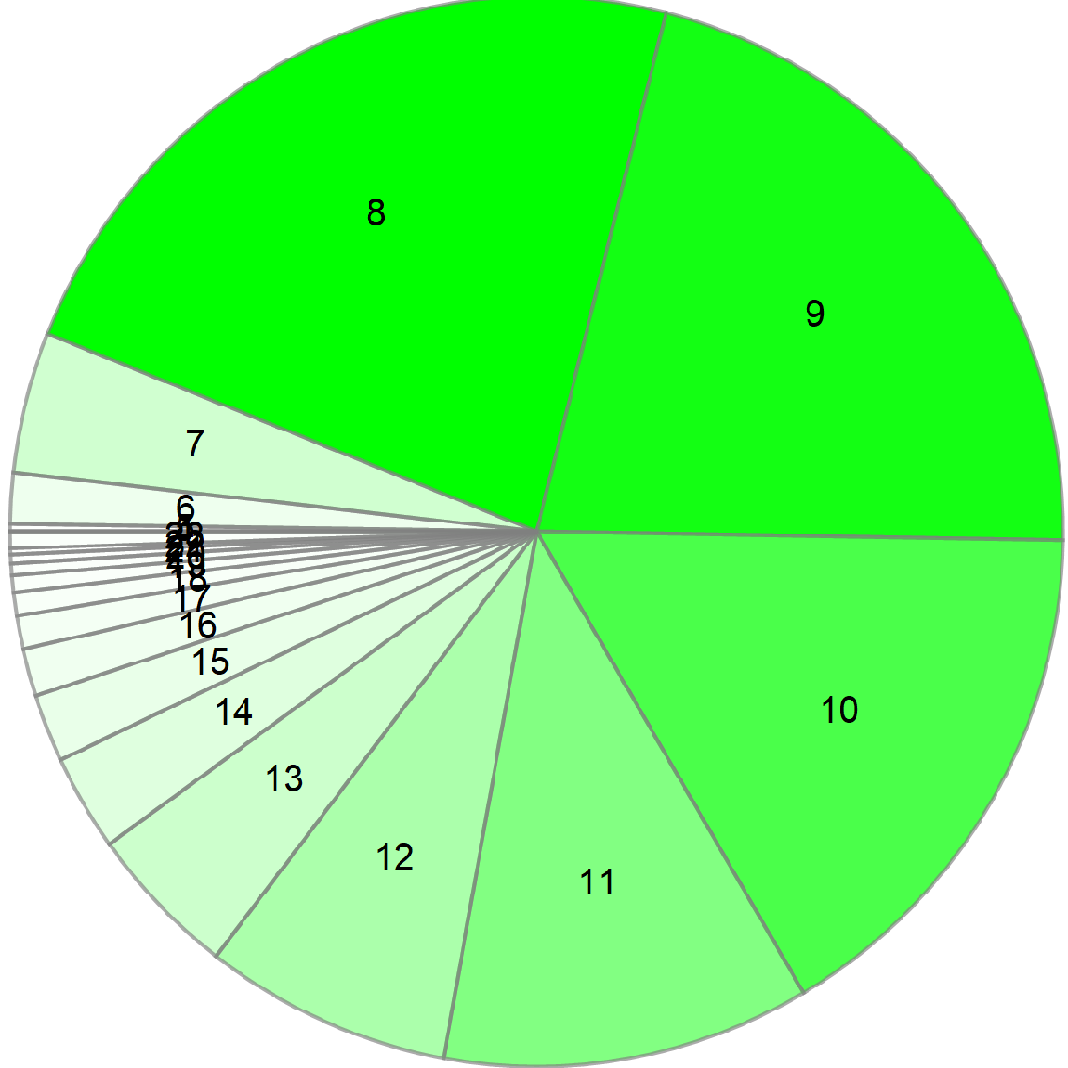
We begin our investigations with the case, where varies in the interval and we take and . In Fig. 3, the BoA for libration points are depicted by five different colours. Also, the BoA cover all of the configuration plane . Most importantly, we notice that a slight change in the value of the parameter , the geometry of the basins changes significantly. In particular, the change in Fig. 3 (a) to Fig. 3(b) can be seen. Here the region of liberation point L5 (green) in the upper part of Fig. 3 (a) shrunk significantly in Fig. 3 (b) due to little change in the value of . A similar observation can be seen for the basin corresponding to liberation point L4 (pink) in the bottom of the figures. When the value of is changing from to till , a major change is observed in Fig. 3(a) to Fig. 3 (f). Despite having the same number of initial conditions converging towards L4 and L5, there is a regular change in the shape of BoA for different values of . The domain of convergence of libration point L1 extends towards infinity whereas the domain of convergence due to libration points L2, L3, L4 and L5 is finite for such values of . Further, we observe that basins for libration points L2 and L3 have the shape like insect with legs and antennas. Also, the shape of BoA corresponding to libration points L4 and L5 appears as many wings of a butterfly. In Fig. 4 (a-f), we have shown Pie-Chart for the number of iterations needed for all initial conditions taken in the configuration plane . In Fig. 4 (a), it is clear that the maximum number of iterations needed are 8, 9 and 10 . Likewise, we have recorded the number of iterations taken by initial conditions to converge for different values of . We notice that approximately 95 % of the initial conditions converge after 25 iterations. A maximum number of initial conditions converge after 8 to10 number of iterations.
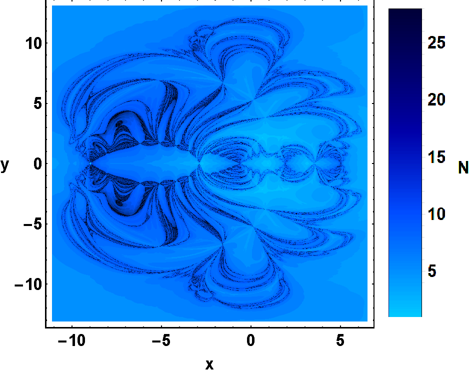
In Fig. 5 (a-f) the relationship between numbers of iterations needed and the initial conditions considered in the configuration plane has been established. The blue tone is used to represent the iterations needed for each initial condition. We notice that the initial conditions along the boundaries of the basins require more iterations than other initial conditions. In Table 1, we have mentioned the details of convergence of initial conditions towards the libration points L1, L2, L3, L4 and L5. The value of basin entropy and boundary basin entropy is also given in Table 1 for different values of . Based on Table 1, Fig. 3, Fig. 4 and Fig. 5, we sum up the following things:
-
•
Due to changes in the value of , if we move from Fig. 3(a) to Fig. 3(f), we observe a significant change in the geometry of BoA.
-
•
The region occupied by the initial conditions converging towards L4 and L5 are approximately equal for each case, although their geometry is changing in every case (see Table 1).
-
•
In all cases, the maximum number of iterations required for the convergence of of the initial conditions are below 25. To achieve the desired accuracy, i.e. of order , the maximum probable number of iterations lies between 8 to 10 (See Fig. 4(a-f)).
-
•
From Table 1, we see that the value of basin entropy and boundary basin entropy is greater than and therefore the existence of fractal is verified. The value of boundary basin entropy is higher than the entropy of other regions indicates the existence of higher fractal regions along the boundaries. From Table 1 and Fig. 5, we conclude that the initial conditions which lie within the fractal regions require more iterations to converge.
4.2 Influence of and
Number of initial conditions converging towards different libration points and the values of entropy and due to variation in parameters and . =2 is fixed. , , , Total Points L1 L2 L3 L4 L5 Execution Time 0.08, 2.0, 0.04, 0.6 1012300 476105 104226 19413 206381 206195 2368.86 0.806377 0.930766 0.06, 1.8, 0.06, 0.8 1043359 477939 93673 28561 221538 221648 2628.81 0.941639 1.06536 0.04, 1.6, 0.08, 1.0 1073073 595431 63702 30089 191832 192019 1812.15 0.861113 0.985576 0.02, 1.4, 0.1, 1.2 1037341 532105 46465 42676 208134 207961 2552.17 0.661595 0.882299 0.01, 1.2, 0.12, 1.4 1011026 482757 37538 60105 215528 215098 3539.01 0.970159 1.05315 0.008, 1.0, 0.14, 1.6 1020700 527815 27792 72293 196344 196456 2429.71 0.948648 1.06536
|
 |
| (a) | (b) |
 |
 |
| (c) | (d) |
 |
 |
| (e) | (f) |
 |
 |
| (a) MINo.=9 | (b) MINo.=9 |
 |
|
| (c) MINo.=7 | (d)MINo.=7 |
 |
 |
| (e) MINo.=7 | (f) MINo.=8 |
|
 |
| (a) | (b) |
 |
 |
| (c) | (d) |
 |
 |
| (e) | (f) |
We continue our investigations with another case where the masses of a nucleus and the disk of a galaxy (G1) is decreasing and the masses of nucleus and the disk of galaxy G2 is increasing. We have displayed BoA for six values in Fig. 6(a-f). In all cases, the value of is fixed. In Fig. 7(a-f), the Pie-chart related to different parameters is displayed. Fig.8(a-f) comprises of the different graphs representing the iterations needed for each initial conditions.
Further, in Fig. 6(a-f), we notice that the BoA for L2 is decreasing, and for L3, it is increasing due to variation in parameters. We observe in Fig. 6(a) few small regions in the left part which disappeared in the next Fig. 6(b) due to change in parameters. We notice such changes or other when we move from Fig. 6(a) to Fig. 6(f). Similar to the previous case, the BoA corresponding to L1 extends to infinity. The BoA of L4 and L5 remain more or less the same in all cases. The shape of BoA of libration points L4 and L5 looks like many butterfly wings. We also observe that the BoA of libration points L2 and L3 have the shape like insects with legs and antennas.
Similar to Table 1, Table 2 comprises the number of initial conditions converging towards different libration points. The value of basin entropy and boundary basin entropy is also given in Table 2. By Table 2, it is evident that the almost entire region in the BoA (except one case) is fractal. The value of is more than the value of indicates the presence of more fractal regions along the boundaries.
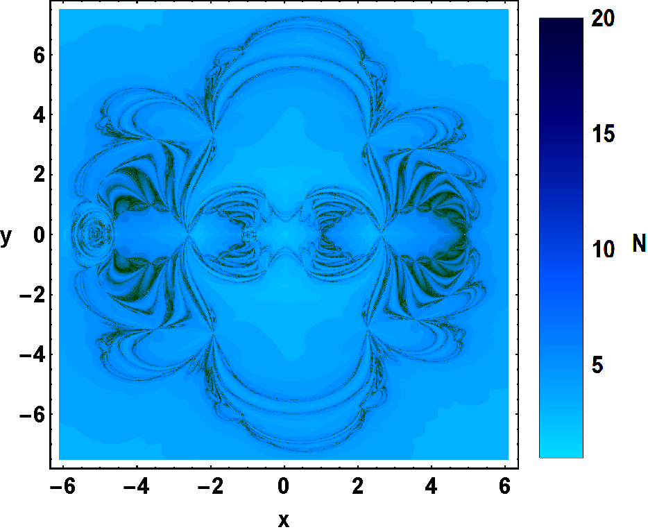
The number of iterations needed for convergence towards libration points for all initial conditions varies from 5 to 30. The distribution of iterations is shown using Pie-chart in Fig. 7 (a-f). The maximum probable iterations are 7 or 8 or 9 in almost all cases. Similar to the case I, 95% initial conditions converge in 25 iterations. The number of iteration needed to convergence for each initial condition is displayed in Fig. 8(a-f). The number of required iterations is presented using a blue tone, i.e., deep blue tone represents more iteration than faded blue tone. This figure gives us a clear idea of the regions where there is a need for more number of required iterations. We summaries followings from Table 2, Fig. 6, Fig. 7 and Fig. 8.
The total area covered by BoA corresponding to L2, L3, L4 and L5 are finite whereas the area covered by a BoA of libration point L1 extends to infinity. The configuration plane is filled by BoA completely.
All initial conditions are converging towards one of the five libration points with the accuracy . We do not find any non-converging points.
Except for one value of a parameter, the existence of fractal is verified by the values of basin entropy given in Table 2. However, in this particular case, the boundaries of BoA are fractal. In all other cases, there is a presence of highly fractal regions along the boundaries (See Table 2 and Fig. 8(a-f)).
In all cases, the maximum number of iterations needed for the convergence of of the initial conditions are below 15. The maximum probable number of iterations needed to achieve the desired accuracy lies between 7 to10.
5 Concluding Remarks
The novelty and importance of this work are clear from the fact that we have chosen this model for the first time to study the BoA and the measure of uncertainty involved in it. Besides this, we have investigated the existence of fractal regions in BoA. The binary system of interacting galaxies has been explored in the framework of the Circular Restricted Three-Body Problem. The parametric evolution of libration points is shown in Fig. 1. The impact of Jacobi’s constant on the geometry of zero-velocity curves is shown in Fig. 2. The multivariate form of the NR method is used to find the convergence of initial conditions towards libration points (act as attractors in the present case). With the help of shape of basins, the influence of parameters and , is analysed (Fig. 3 and 5). The data obtained from numerical simulations is given in Table 1 and Table 2, which reflects the originality of this work. Table 1 and Table 2 comprises of the details convergence of initial conditions towards libration points; time consumed by CPU; the value of basin entropy and boundary basin entropy. The number of iterations needed for the convergence of the initial conditions is shown using Pie-chart (in the tone of green colour) in Fig. 4 and Fig. 7, which is useful, informative and different from earlier works. Further, we have established the relationship between the number of iterations required for convergence and the set of initial conditions on configuration plane (Fig. 5 and 8).
For all numerical simulations, we have used a machine configured with Intel(R) Core(TM) i7-8550U CPU 1.80 GHz. In all cases, the computational time of the CPU is less than or equal to one hour for the simulation a uniform grid of 10241024 initial conditions (nearly ten lakhs). The time taken by the CPU to classify all initial conditions is less than one minute. We have considered six different values of all the parameters. The results of simulations can be summarized as follows: {itemlist}
The programming for the computation of BoA; basin entropy and plotting of all graphs is done on Mathematica. The execution time taken by CPU for BoA and the classification of initial conditions in this model is explicitly mentioned in Table 1 and Table 2. As per data available from earlier works, the time mentioned in Table 1 and Table 2 is comparatively less.
In almost all cases, we find that configuration plane contains the combinations of fractal regions and distinct BoA. If we choose an initial condition in these regions, it is challenging to predict the convergence towards a specific libration point. The unpredictability of basin of attraction is due to the non-linearity of the expressions of the potential responsible for the motion of a star in the presence of the two interacting galaxies (G1 and G2) (See equation (4)) ). These regions are mainly located along with the neighbourhood of boundaries of BoA.
The area enclosed by BoA corresponding to libration points L2, L3, L4 and L5 are finite whereas, the area associated with central libration point L1 extends to infinity. Also, the area of basins corresponding to L4 and L5 are approximately the same for all cases. The area of basins corresponding to L2 and L3 changes due to variation in the parameters.
Based on simulations, we observe that all the initial conditions (10 lakhs approx.) on a uniform grid of 10241024 converge to any one of the five libration points of the dynamical system with an accuracy of order . We do not find any non-converging initial condition. (See Table 1 and Table 2)
Fig. 5 (a-f) and Fig. 8 (a-f) reveal that all initial conditions which require more iterations lie along the boundaries of BoA, i.e., along with the fractal regions as compare to Initial conditions lying away from boundaries.
Due to a decrease in the mass of the galaxy (G1) and the increase of the mass of the galaxy (G2), the area of a BoA due to L2 decreases and the area of a BoA due to L3 increases. However, the region occupied by BoA due to L4 and L5 is roughly the same for all cases. (See Fig. 6 (a-f))
By Table 1 and Table 2, we find that the values of entropy and is greater than except for one value of in Table 2. Thus all BoA are fractal and there is an existence of highly fractal regions along the boundaries.
The maximum number of iteration that an initial condition needs to converge towards libration points lie between 7-10 for all cases. (See Fig. 4 (a-f)and Fig. 7 (a-f)).
The parameters have a significant impact on the evolution of libration points as well as the geometry of zero-velocity curves.
We observe very few research works in the area of space dynamics. That is why we have considered a galactic model for our work. These results will be useful for many researchers to work in these models. On the other hand, these observations give us an intuitive idea for the existence of some properties (like a different type of basins, the existence of Wada basin ). In future, we will try to investigate these properties in other complex nonlinear models in the field of space dynamics and celestial mechanics.
References
- Alvar [2016] Daza, Alvar et al. [2016], Basin entropy: a new tool to analyze uncertainty in dynamical systems. Scientific Reports, 6, 31416.
- Alvar [2017] Daza, Alvar et al. [2017], Chaotic dynamics and fractal structures in experiments with cold atoms, Phys. Rev. A 95, 013629.
- Alvar [2018] Daza, Alvar et al. [2018], Basin Entropy, a Measure of Final State Unpredictability and Its Application to the Chaotic Scattering of Cold Atoms, Chaotic, Fractional, and Complex Dynamics: New Insights and Perspectives. Understanding Complex Systems, 9-34.
- Hasan et al. [1993] Hasan, H., Pfenniger, D. and Norman, A. C. [1993], Galactic bars with central mass concentrations three-dimensional dynamics, APJ, 409, 91.
- Kalvouridis et al. [2012] Kalvouridis, T. and Gousidou-Koutita, M. [2012], Basins of Attraction in the Copenhagen Problem Where the Primaries Are Magnetic Dipoles, Applied Mathematics,3, 6, 541-548.
- Kumar [2016] Kumar, Vinay, Gupta, Beena R & Aggarwal, R. [2016], Numerical Investigation of a Star’s Trajectory in Binary Quasar System, Advanced Studies in Contemporary Mathematics, 26, 3.
- Latewe [2007] Latewe, G., Magain, P., and Courbin, F. et al. [2007], On-axis spectroscopy of the host galaxies of 20 optically luminous quasars at , MNRAS, 378, 1, 83-108.
- Miyamoto and Nagai [1975] Miyamoto, W. and Nagai, R. [1975],Three-dimensional models for the distribution of mass in galaxies, PASJ, 27, 533.
- Sillianpaa et al. [1988] Sillanpaa, A., Haarala, S. and Valtonen, M. J. [1988], OJ 287- Binary pair of supermassive black holes, APJ, 325, 628.
- Sprott et al. [2015] Sprott, J. C. and Xiong, A. [2015], Classifying and quantifying basin of attraction, Chaos: An Interdisciplinary Journal of Nonlinear Science, 25, 8.
- Wolfram [2017] Wolfram Research, Inc. [2014], Mathematica, Version 11.0.1, Champaign, IL.
- Suraj [2019] Sanam Suraj, Md., Sachan, Prachi., Zotos E. E., Mittal, A., Aggarwal, R.,[2019], On the Newton–Raphson basins of convergence associated with the libration points in the axisymmetric restricted five-body problem: Int. J. Non-Linear Mech., 112, 25-47.
- Zotos [2012] Zotos., E. E. [2012], Order and chaos in three dimensional binary system of interacting galaxies, APJ, 750, 56.
- Zotos [2017] Zotos, E. E. [2017a], Revealing the basins of convergence in the planar equilateral restricted four-body problem. Astrophys. Space Sci. 362, 2.
- Zotos [2018] Zotos E. E., Kumar Satya S., Aggarwal, R. and Sanam Suraj, M. [2018], Basins of Convergence in the Circular Sitnikov Four-Body Problem with Nonspherical Primaries, Int. J. of Bifurcation and Chaos, 28, 05, 1830016.