FracGM: A Fast Fractional Programming Technique for Geman-McClure Robust Estimator

Robust estimation problems are usually reformulated as iterative weighted least squares problems [15, 28]. In Geman-McClure robust estimations, most approaches rely on Black-Rangarajan duality [29], which is a weighted least squares with an additional regularization term [30, 17, 31]. For example, Graduated Non-Convexity (GNC) [17] proposes a general-purpose robust solver for both truncated least squares (TLS) and Geman-McClure (GM) robust cost in conjunction with such duality technique, and introduces an approximation optimization process from convexity to non-convexity. With recent advances of semidefinite relaxation [32], there are also approaches to recast Geman-McClure robust functions to semidefinite programming (SDP) [21].

Unlike the robust estimators based on the Black-Rangarajan duality and semidefinite relaxation Geman-McClure, FracGM leverages Dinkelbach’s transform [23] and the Lagrangian to reformulate the problem as an underlying convex program with additional auxiliary variables. It was originally introduced in the field of fractional programming optimization [23, 24, 25, 26], while to the best of our knowledge, FracGM is the first approach to apply such technique for Geman-McClure robust estimation.

Point cloud registration is the process of aligning two point clouds by finding a spatial rigid transformation. Horn [33] first proposes a closed-form solution by decoupling the problem to scale, rotation and translation sub-problems. With advances of relaxation techniques in recent decades, Olsson and Eriksson [34] apply Lagrangian duality with semidefinite relaxation. In addition, Briales and Gonzalez-Jimenez [35] introduce orthonormality and determinant constraints such that the relaxation is empirically tight. Those methods are said to be outlier-free approaches, since they assume that all measurement noises are modeled under ordinary Gaussian distributions.

In real-world applications, however, there are outlier measurements which may interfere with estimation accuracy. For the purpose of mitigating the impact of outliers, robust estimation becomes a promising strategy in point cloud registration to identify and isolate bad measurements. Zhou et al. [31] propose the idea to solve robust registration by gradually adjusting the Geman-McClure robust function. Yang et al. [9] develop Truncated least squares Estimation And SEmidefinite Relaxation (TEASER), where they reformulate the problem to large-scale SDP. They also develop a fast implementation TEASER++ by leveraging GNC rotation solver to prevent large computational cost in SDP.

We write an equivalent problem for Problem (4) by introducing upper bound variable $\boldsymbol{\beta}\in\mathbb{R}^{N}$:

With Dinkelbach’s transform [23] and Lagrangian, the following \threflemma_1 derives an underlying convex problem of the equivalent Problem (5). It also claims the relationship between the minimizer of Problem (4) and newly introduced auxiliary variables $\boldsymbol{\beta}$ and $\boldsymbol{\mu}$.

In this way, the primal problem (5) turns out to be finding a feasible solution $\bar{\boldsymbol{x}}$ of the dual problem (6) as well as auxiliary variables $(\bar{\boldsymbol{\beta}},\bar{\boldsymbol{\mu}})$. We resort to alternating minimization that iteratively and separately updates $\boldsymbol{x}$ and $(\boldsymbol{\beta},\boldsymbol{\mu})$. Specifically, in the $k$-th iteration, given a fixed $(\boldsymbol{\beta}^{k},\boldsymbol{\mu}^{k})$ that satisfies the auxiliary variable constraints $\boldsymbol{\mu}^{k}_{i}>0$ and $c^{2}>\boldsymbol{\beta}^{k}_{i}$, solving $\boldsymbol{x}^{k}$ with Problem (6) becomes a convex programming with fixed variable dimension $\mathbb{R}^{d}$. As for finding $(\boldsymbol{\beta}^{k+1},\boldsymbol{\mu}^{k+1})$ with given $\boldsymbol{x}^{k}$, a root finding problem is introduced in the next section. It is same as Jong’s approach [24], whereas we will additionally claim that the auxiliary variable constraints is theoretically preserved during the optimization.

Let $\boldsymbol{\alpha}=(\boldsymbol{\beta}^{\top},\boldsymbol{\mu}^{\top})^{\top}\in\mathbb{R}^{2N}$ denote the auxiliary variables, let $\boldsymbol{x}_{\boldsymbol{\alpha}}$ be the solution of problem (6) given an $\boldsymbol{\alpha}$, and $r_{i}(\boldsymbol{x}_{\boldsymbol{\alpha}}),\ i=1,\dots,N$ are the corresponding residuals. Define a function $\psi:\mathbb{R}^{2N}\times\mathbb{R}^{d}\to\mathbb{R}^{2N}$ as follows:

This function is specifically defined by the constraints (7) and (8) such that $\psi(\bar{\boldsymbol{\alpha}},\bar{\boldsymbol{x}})=\mathbf{0}$, where $\bar{\boldsymbol{\alpha}}=(\bar{\boldsymbol{\beta}}^{\top},\bar{\boldsymbol{\mu}}^{\top})^{\top}$ and $(\bar{\boldsymbol{x}},\bar{\boldsymbol{\beta}},\bar{\boldsymbol{\mu}})$ is the solution of Problem (6). By [24, Corollary 2.1], if $\bar{\boldsymbol{x}}$ is a solution of Problem (4), then there exists $\boldsymbol{\alpha}\in\mathbb{R}^{2N}$ such that $\bar{\boldsymbol{x}}=\boldsymbol{x}_{\boldsymbol{\alpha}}$ and

This shows that a solution of the auxiliary variables $\boldsymbol{\alpha}$ can be obtained by solving $\psi(\boldsymbol{\alpha},\boldsymbol{x}_{\boldsymbol{\alpha}})=\mathbf{0}$. \threfthm next states that such solution satisfies the KKT conditions in \threflemma_1.

thm provides an assurance that all $\boldsymbol{x}_{\bar{\boldsymbol{\alpha}}}$ such that $\psi(\bar{\boldsymbol{\alpha}},\boldsymbol{x}_{\bar{\boldsymbol{\alpha}}})=\mathbf{0}$ is a solution candidate for Problem (4) that satisfies necessary optimality conditions, and also guarantees that we can indeed use Jong’s approach [24] to obtain a solution in our case where numerators and denominators of the fractional program are all convex. To this end, given a fixed $\boldsymbol{\alpha}^{k}=((\boldsymbol{\beta}^{k})^{\top},(\boldsymbol{\mu}^{k})^{\top})^{\top}$ that satisfies the auxiliary variable constraints, we solve the convex program (6) and obtain $\boldsymbol{x}^{k}=\boldsymbol{x}_{\boldsymbol{\alpha}^{k}}$. If $\psi(\boldsymbol{\alpha}^{k},\boldsymbol{x}^{k})=\mathbf{0}$, by \threfthm, FracGM converges to a local solution of Problem (4). Otherwise, we update $\boldsymbol{\alpha}$ by solving $\psi(\boldsymbol{\alpha},\boldsymbol{x}^{k})=\mathbf{0}$, where $\boldsymbol{x}^{k}=\boldsymbol{x}_{\boldsymbol{\alpha}^{k}}$ is the fixed solution of Problem (6) from the previous iteration in the sense of alternating minimization. Clearly, Problem (9) is a linear system with fixed $\boldsymbol{x}^{k}$, we write the closed-form solution $\boldsymbol{\alpha}^{k+1}$ component-wise as follows:

In summary, we iteratively update $\boldsymbol{\alpha}^{k}$ by Equation (10) and solve $\boldsymbol{x}^{k}$ by Problem (6) until the stopping criteria: $\psi(\boldsymbol{\alpha}^{k},\boldsymbol{x}^{k})=\mathbf{0}$. Note that during the $k^{\prime}$-th iteration that hasn’t converge yet, $\boldsymbol{\alpha}^{k^{\prime}}$ is the solution of $\psi(\boldsymbol{\alpha},\boldsymbol{x}^{k^{\prime}-1})=\mathbf{0}$ from the previous iteration, however, not the solution of $\psi(\boldsymbol{\alpha}^{k^{\prime}},\boldsymbol{x}^{k^{\prime}})=\mathbf{0}$ in the current iteration. This stopping criteria can also be interpreted as finding an $\boldsymbol{\alpha}^{k}$ such that both Problem (6) and Problem (9) are solved. The complete procedure is depicted in Algorithm 1.

In Section III-A and III-B, we have shown that the solution of FracGM is a KKT point of Problem 6 by \threfthm, which is a local solution of Problem (5) by \threflemma_1. It follows from [24, Corollary 2.1] that if Problem (9) has only one solution, then such unique solution is the optimal solution of Problem (5). Consequently, we derive the following statement from the uniqueness of Problem (9) [24, Theorem 3.1]:

An example of FracGM satisfying \threfprop, i.e., having theoretically global optimal guarantees, is given in the supplementary material.

We first discuss about the Wahba’s rotation Problem [27], which is basically a registration of two point clouds that only differ by a 3-D rotation. Let $\{\boldsymbol{a}_{i}\},\{\boldsymbol{b}_{i}\}$ be two sets of point clouds with $N$ points, source set and target set, where $\boldsymbol{a}_{i},\boldsymbol{b}_{i}\in\mathbb{R}^{3}$ are 3-D points. The goal is to find a rotation matrix $\mathbf{R}$ between the two point clouds, i.e., $\boldsymbol{b}_{i}=\mathbf{R}\boldsymbol{a}_{i}+\boldsymbol{\varepsilon}_{i}$, with error terms $\boldsymbol{\varepsilon}_{i}\sim\mathcal{N}(0,\sigma_{i}^{2}\mathbf{I}_{3})$ following the isotropic Gaussian distribution. The maximum likelihood estimation is equivalent to the following least squares problem:

We first rewrite it as a quadratic program:

where $\mathbf{M}_{i}=[\boldsymbol{a}_{i}^{\top}\otimes\mathbf{I}_{3},-\boldsymbol{b}]^{\top}[\boldsymbol{a}_{i}^{\top}\otimes\mathbf{I}_{3},-\boldsymbol{b}]\in\mathbb{R}^{10\times 10}$, $\boldsymbol{x}=[\text{vec}(\mathbf{R})^{\top},1]^{\top}\in\mathbb{R}^{10}$, $\text{vec}(\mathbf{R})\in\mathbb{R}^{9}$ is the column-wise vectorization of the rotation matrix $\mathbf{R}$, and $\boldsymbol{e}_{10}=(0,\dots,0,1)^{\top}\in\mathbb{R}^{10}$. This vectorization and homogenization technique is commonly used [35, 34]. We also remark that all square of residual functions $r_{i}^{2}(\boldsymbol{x})=\boldsymbol{x}^{\top}(\frac{1}{\sigma_{i}^{2}}\mathbf{M}_{i})\boldsymbol{x}$ defined in Problem (12) are twice continuously differentiable and quadratic convex. Next, we apply the GM robust function (2) and form the following optimization problem:

In order to apply FracGM, we relax the $\text{SO}(3)$ constraints to align with the form of Problem (4). Since the numerators and denominators in the relaxed Problem (13) are quadratic, the derived Problem (6) is a quadratic program with only one equality constraint. Such problem has a closed-form solution by Shur complement and the KKT matrix [37]:

After finding a solution $\boldsymbol{x}^{*}$ by FracGM, we dehomogenize $\bar{\boldsymbol{x}}\in\mathbb{R}^{10}$ to $\bar{\boldsymbol{x}}^{\prime}\in\mathbb{R}^{9}$, then reshape it to a matrix $\mathbf{R}^{\prime}\in\mathbb{R}^{3\times 3}$. Since the solution is on the relaxed convex space and we are agnostic on theoretical conditions of tightness, we forcibly project it back to the special orthogonal space by SVD [38]. This technique is also commonly used after linear relaxation in rotation estimation [35, 34]. In light of an initial guess is needed for FracGM, we simply use the fast closed-form solution [33] for Problem (11). Despite that this closed-form solution does not tolerate outliers, we will show that it is proficient even when there are numerous outliers in Section V. We summarize the FracGM-based rotation solver in Algorithm 2.

We extend the FracGM-based rotation solver to a registration solver, which is to find the spatial transformation between the two point clouds, i.e., $\boldsymbol{b}_{i}=\mathbf{R}\boldsymbol{a}_{i}+\boldsymbol{t}+\boldsymbol{\varepsilon}_{i}$, where $\mathbf{R}$ is the rotation matrix, $\boldsymbol{t}$ is the translation vector, and error terms $\boldsymbol{\varepsilon}_{i}\sim\mathcal{N}(0,\sigma_{i}^{2}\mathbf{I}_{3})$ follow the isotropic Gaussian distribution. In this way, we get the following problem:

We extend Problem (13) to solving spatial transformation and the problem formulation of GM robust point cloud registration becomes:

where $\mathbf{M}_{i}=[\boldsymbol{a}_{i}^{\top}\otimes\mathbf{I}_{3},\mathbf{I}_{3},-\boldsymbol{b}]^{\top}[\boldsymbol{a}_{i}^{\top}\otimes\mathbf{I}_{3},\mathbf{I}_{3},-\boldsymbol{b}]\in\mathbb{R}^{13\times 13}$, $\boldsymbol{x}=[\text{vec}(\mathbf{R})^{\top},\boldsymbol{t}^{\top},1]^{\top}\in\mathbb{R}^{13}$. The structural consistency between Equation (13) and Equation (16) permits a similar algorithm to solve the registration problem. In particular, the algorithm of FracGM for point cloud registration can be extended from Algorithm 2 by adding an initial guess $(\mathbf{R}^{0},\boldsymbol{t}^{0})$ and solving $\boldsymbol{x}^{*}\in\mathbb{R}^{13}$ in Problem (16).

It is worth noting that the introduced FracGM-based registration solver directly estimates the relative transformation between two point clouds, whereas TEASER [9] decouples rotation and translation estimation. This strategy is more computationally efficient, as it avoids the increase in measurement number complexity up to $O(N^{2})$ when introducing translation-invariant measurements for rotation solvers. In addition, this computational cost-friendly strategy also improves the accuracy of estimation results.

We acknowledge that the theoretical guarantee of global optimality for FracGM-based rotation and registration solvers remains an open issue. Specifically, the global optimality is subjected to variable space relaxation tightness and \threfprop for the relaxed program, which could be challenging to verify as it depends on the input data. It requires further investigation to address the issue¹¹1Empirical studies on global optimality including relaxation tightness and sensitivity to initial guesses are available at the supplementary material..

We evaluate the resistance to outliers in different outlier rates of the proposed FracGM rotation solver. In practice, we down sample the Stanford Bunny point cloud to $50$ points for outlier rates between 20% and 80%, and to $500$ points for outlier rates higher than 80%. We construct the corresponding point cloud by adding a Gaussian noise with standard deviation of 0.01, and applying random rotation $\mathbf{R}\in\text{SO}(3)$. We generate outliers by replacing a fraction (outlier rate) of points by random sampled 3-D points inside the sphere of radius 2. The threshold $c$ in robust functions (TLS and GM) are all set to 1.

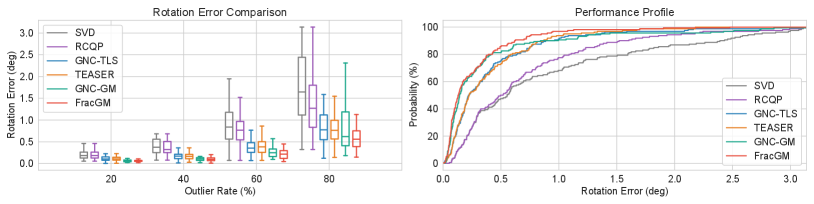
Figure 2 shows the box plot of error comparison and performance profile to evaluate rotation solvers. For outlier rates between 20% and 80%, FracGM has the lowest mean rotation error of $0.26^{\circ}$ and the highest probability of being the optimal solver than both outlier-free solvers and outlier-awareness solvers. FracGM stands out in extreme cases where the outlier rate is greater than 90%. In contrast to other solvers that can only limit up to 60% of rotation errors within 1 degree, FracGM confines approximately 80% of rotation errors within this range.

We also compare the error curve with TLS- and GM-based GNC [17] in Figure 3. It reveals that FracGM not only has a better convergence speed than GNC approaches, but also a lower error. We believe that GNC approximates the non-convex objective by some surrogate functions, in which such approximation might be far from the non-convex objective in the early iterations. On the other hand, our solver reformulates the non-convex objective to an equivalent convex problem, thus we are solving the exact same objective in every iteration. Thus, FracGM has a better ability to deal with outliers and can obtain a higher-quality estimation.

We evaluate the proposed FracGM registration solver under two different scenarios. In the first scenario, we down sample the Stanford Bunny point cloud to 500 points and manipulate different rates of outlier point correspondences from 20% to 80%, which is the same configuration of Section V-A with additional random translation $\boldsymbol{t}\in\mathbb{R}^{3},\|\boldsymbol{t}\|\leq 1$. We set the noise bound [9] of TEASER++ and FracGM ($\sigma_{i}$ in Equation (16)) to 0.1, while RANSAC and FGR does not consider $\sigma_{i}$ in their problem formulation. In the second scenario, we solve the problem given different noise bound guess to evaluate the impact of it. We believe that specifying the above two configurations are important in the registration task, since the error modeling of outlier in real-world applications is usually unknown and diverse.

We notice that FGR first filters bad correspondence by Fast Point Feature Histogram (FPFH) and nearest neighbors search, while TEASER++ has a Maximum Clique Inlier Selection (MCIS) step to prune outliers before estimating. Both techniques serve as correspondence preprocessing, and since the main idea of robust estimator is to deal with outliers by the solver itself, we exclude both steps in order to demonstrate the robustness of each solver.

Figure 1 demonstrates an example of this experiment. We run RANSAC for 100 times, which is a multi-times non-robust solver, while others are one-time robust solvers. Figure 4 reports that FracGM is the only one that is truly robust to outliers and can really work well with larger outlier rate without any correspondence preprocessing or outlier pruning. As the outlier rate increased from 20% to 80%, the rotation and translation error of TEASER++ escalated by 186% and 900%, while FracGM increased only by 87% and 106%, representing an improvement of 53% and 88%, respectively. As stated in Section IV-B, we also extended a FracGM translation solver to adapt the decoupled structure of TEASER++. Figure 4 shows that the results of rotation estimation in FracGM (decouple) is similar to FracGM, while the accuracy of translation estimation in FracGM (decouple) falls. This is because the measurements for the decoupled translation solver are affected by the prior rotation estimation, and fixing a rotation matrix may cause the translation solver converge to some local solution. Table I reports that the computation time of FracGM (decouple) increases exponentially due to the fact that the measurements for the decoupled rotation solver also increases exponentially, while FracGM can deal with thousands of measurements with milliseconds.

In the above experiments, we choose a noise bound (the upper bound of $\sigma_{i}$ in Equation (16)) of 0.1 that is larger than the noise standard deviation of the data set at $0.01$. However, we may not know the actual noise of the measurements in reality, and thus we tend to set a larger noise bound guess. Figure 5 reports the result of setting different noise bounds on a fixed dataset with 50% of outliers, while the other settings are the same as before. It could be expected that the estimation will be more accurate if the noise bound is closer to the actual noise standard deviation. Despite this, the estimation error of TEASER++ increases dramatically. For example, given a noise bound of 1 that is 100 times the noise standard deviation, FracGM has a 66% and 62% improvement over TEASER++ in terms of rotation and translation error.

We test our proposed FracGM registration solver on the realistic 3DMatch dataset [39] to examine the real-world application capability. We downsample point clouds with a voxel size of 5 cm, obtain the correspondence by FPFH, perform a nearest-neighbor search to generate sets of point correspondences and filter them with MCIS [9].

Table II exhibits the registration accuracy and computational time between our solver and other state-of-the-art methods (RANSAC [42], FGR [31] and TEASER++ [9]). FracGM has the lowest average rotation error within $1.22^{\circ}$ and an average translation error less than 1.7 m. Since our solver converges fast and we only solve a fixed low-dimensional quadratic program and a linear equation system during each iteration, FracGM can be executed in real-time with an average of 25 milliseconds each registration. In terms of rotation and translation errors across 9 tested scenes, FracGM achieves the best results in 13 out of 18 outcomes, while having a 19.43% improvement of computation time compared to TEASER++.

References

- [1] A. Chatterjee and V. M. Govindu, “Efficient and robust large-scale rotation averaging,” in ICCV. IEEE Computer Society, 2013, pp. 521–528.
- [2] ——, “Robust relative rotation averaging,” IEEE Trans. Pattern Anal. Mach. Intell., vol. 40, no. 4, pp. 958–972, 2018.
- [3] R. I. Hartley, K. Aftab, and J. Trumpf, “L1 rotation averaging using the weiszfeld algorithm,” in CVPR. IEEE Computer Society, 2011, pp. 3041–3048.
- [4] L. Wang and A. Singer, “Exact and stable recovery of rotations for robust synchronization,” Information and Inference: A Journal of the IMA, vol. 2, no. 2, pp. 145–193, 2013.
- [5] Z. Deng, Y. Yao, B. Deng, and J. Zhang, “A robust loss for point cloud registration,” in ICCV. IEEE, 2021, pp. 6118–6127.
- [6] A. W. Fitzgibbon, “Robust registration of 2d and 3d point sets,” Image Vis. Comput., vol. 21, no. 13-14, pp. 1145–1153, 2003.
- [7] H. M. Le, T. Do, T. Hoang, and N. Cheung, “SDRSAC: semidefinite-based randomized approach for robust point cloud registration without correspondences,” in CVPR. Computer Vision Foundation / IEEE, 2019, pp. 124–133.
- [8] J. Ma, J. Zhao, J. Tian, Z. Tu, and A. L. Yuille, “Robust estimation of nonrigid transformation for point set registration,” in CVPR. IEEE Computer Society, 2013, pp. 2147–2154.
- [9] H. Yang, J. Shi, and L. Carlone, “TEASER: fast and certifiable point cloud registration,” IEEE Trans. Robotics, vol. 37, no. 2, pp. 314–333, 2021.
- [10] L. Carlone and G. C. Calafiore, “Convex relaxations for pose graph optimization with outliers,” IEEE Robotics Autom. Lett., vol. 3, no. 2, pp. 1160–1167, 2018.
- [11] G. H. Lee, F. Fraundorfer, and M. Pollefeys, “Robust pose-graph loop-closures with expectation-maximization,” in IROS. IEEE, 2013, pp. 556–563.
- [12] N. Sünderhauf and P. Protzel, “Towards a robust back-end for pose graph SLAM,” in ICRA. IEEE, 2012, pp. 1254–1261.
- [13] J. Beuchert, M. Camurri, and M. F. Fallon, “Factor graph fusion of raw GNSS sensing with IMU and lidar for precise robot localization without a base station,” in ICRA. IEEE, 2023, pp. 8415–8421.
- [14] T. Suzuki, “Attitude-estimation-free GNSS and IMU integration,” IEEE Robotics Autom. Lett., vol. 9, no. 2, pp. 1090–1097, 2024.
- [15] M. Bosse, G. Agamennoni, and I. Gilitschenski, “Robust estimation and applications in robotics,” Found. Trends Robotics, vol. 4, no. 4, pp. 225–269, 2016.
- [16] L. Lu, W. Wang, X. Yang, W. Wu, and G. Zhu, “Recursive geman-mcclure estimator for implementing second-order volterra filter,” IEEE Trans. Circuits Syst. II Express Briefs, vol. 66-II, no. 7, pp. 1272–1276, 2019.
- [17] H. Yang, P. Antonante, V. Tzoumas, and L. Carlone, “Graduated non-convexity for robust spatial perception: From non-minimal solvers to global outlier rejection,” IEEE Robotics Autom. Lett., vol. 5, no. 2, pp. 1127–1134, 2020.
- [18] C. Zach, “Robust bundle adjustment revisited,” in ECCV. Springer, 2014, pp. 772–787.
- [19] F. Dellaert and M. Kaess, “Factor graphs for robot perception,” Found. Trends Robotics, vol. 6, no. 1-2, pp. 1–139, 2017.
- [20] D. M. Rosen, M. Kaess, and J. J. Leonard, “RISE: an incremental trust-region method for robust online sparse least-squares estimation,” IEEE Trans. Robotics, vol. 30, no. 5, pp. 1091–1108, 2014.
- [21] M. Castella and J. Pesquet, “Optimization of a geman-mcclure like criterion for sparse signal deconvolution,” in CAMSAP. IEEE, 2015, pp. 309–312.
- [22] H. Yang and L. Carlone, “A quaternion-based certifiably optimal solution to the wahba problem with outliers,” in ICCV. IEEE, 2019, pp. 1665–1674.
- [23] W. Dinkelbach, “On nonlinear fractional programming,” Management Science, vol. 13, no. 7, pp. 492–498, 1967.
- [24] Y. Jong, “An efficient global optimization algorithm for nonlinear sum-of-ratios problem,” Optimization Online, vol. 32, pp. 38–39, 2012.
- [25] I. M. Stancu-Minasian, Fractional programming: theory, methods and applications, 1997, vol. 409.
- [26] S. Schaible and J. Shi, “Fractional programming: The sum-of-ratios case,” Optim. Methods Softw., vol. 18, no. 2, pp. 219–229, 2003.
- [27] G. Wahba, “A least squares estimate of satellite attitude,” SIAM review, vol. 7, no. 3, pp. 409–409, 1965.
- [28] K. MacTavish and T. D. Barfoot, “At all costs: A comparison of robust cost functions for camera correspondence outliers,” in CRV. IEEE Computer Society, 2015, pp. 62–69.
- [29] M. J. Black and A. Rangarajan, “On the unification of line processes, outlier rejection, and robust statistics with applications in early vision,” Int. J. Comput. Vis., vol. 19, no. 1, pp. 57–91, 1996.
- [30] J. T. Barron, “A general and adaptive robust loss function,” in CVPR. Computer Vision Foundation / IEEE, 2019, pp. 4331–4339.
- [31] Q. Zhou, J. Park, and V. Koltun, “Fast global registration,” in ECCV. Springer, 2016, pp. 766–782.
- [32] F. Bugarin, D. Henrion, and J. Lasserre, “Minimizing the sum of many rational functions,” Math. Program. Comput., vol. 8, no. 1, pp. 83–111, 2016.
- [33] B. K. P. Horn, “Closed-form solution of absolute orientation using unit quaternions,” Journal of the Optical Society A, vol. 4, pp. 629–642, 04 1987.
- [34] C. Olsson and A. P. Eriksson, “Solving quadratically constrained geometrical problems using lagrangian duality,” in ICPR. IEEE Computer Society, 2008, pp. 1–5.
- [35] J. Briales and J. G. Jiménez, “Convex global 3d registration with lagrangian duality,” in CVPR. IEEE Computer Society, 2017, pp. 5612–5621.
- [36] R. W. Freund and F. Jarre, “Solving the sum-of-ratios problem by an interior-point method,” J. Glob. Optim., vol. 19, no. 1, pp. 83–102, 2001.
- [37] S. Boyd and L. Vandenberghe, Convex optimization. Cambridge university press, 2004.
- [38] P. H. Schönemann, “A generalized solution of the orthogonal procrustes problem,” Psychometrika, vol. 31, no. 1, pp. 1–10, 1966.
- [39] A. Zeng, S. Song, M. Nießner, M. Fisher, J. Xiao, and T. A. Funkhouser, “3dmatch: Learning local geometric descriptors from RGB-D reconstructions,” in CVPR. IEEE Computer Society, 2017, pp. 199–208.
- [40] G. Turk and M. Levoy, “Zippered polygon meshes from range images,” in SIGGRAPH. ACM, 1994, pp. 311–318.
- [41] R. B. Rusu, N. Blodow, and M. Beetz, “Fast point feature histograms (FPFH) for 3d registration,” in ICRA. IEEE, 2009, pp. 3212–3217.
- [42] M. A. Fischler and R. C. Bolles, “Random sample consensus: A paradigm for model fitting with applications to image analysis and automated cartography,” Commun. ACM, vol. 24, no. 6, pp. 381–395, 1981.