This paper was converted on www.awesomepapers.org from LaTeX by an anonymous user.
Want to know more? Visit the Converter page.

Foundations of Multivariate Distributional Reinforcement Learning

Harley Wiltzer Correspondence to [email protected] Mila — Québec AI Institute McGill University Jesse Farebrother Mila — Québec AI Institute McGill University Arthur Gretton Google DeepMind Gatsby Unit, University College London Mark Rowland Google DeepMind
Abstract

In reinforcement learning (RL), the consideration of multivariate reward signals has led to fundamental advancements in multi-objective decision-making, transfer learning, and representation learning. This work introduces the first oracle-free and computationally-tractable algorithms for provably convergent multivariate distributional dynamic programming and temporal difference learning. Our convergence rates match the familiar rates in the scalar reward setting, and additionally provide new insights into the fidelity of approximate return distribution representations as a function of the reward dimension. Surprisingly, when the reward dimension is larger than 11, we show that standard analysis of categorical TD learning fails, which we resolve with a novel projection onto the space of mass-11 signed measures. Finally, with the aid of our technical results and simulations, we identify tradeoffs between distribution representations that influence the performance of multivariate distributional RL in practice.

1 Introduction

Distributional reinforcement learning [MSK+10, BDM17b, BDR23, DRL] focuses on the idea of learning probability distributions of an agent’s random return, rather than the classical approach of learning only its mean. This has been highly effective in combination with deep reinforcement learning [YZL+19, BCC+20, WBK+22], and DRL has found applications in risk-sensitive decision making [LM22, KEF23], neuroscience [DKNU+20], and multi-agent settings [ROH+21, SLL21].

In general, research in distributional reinforcement learning has focused on the classical setting of a scalar reward function. However, prior non-distributional approaches to multi-objective RL [RVWD13, HRB+22] and transfer learning [BDM+17a, BHB+20] model value functions of multivariate cumulants,111Cumulants refer to accumulated quantities in RL (e.g., rewards or multivariate rewards)—not to be confused with statistical cumulants. rather than a scalar reward. Having learnt such a multivariate value function, it is then possible to perform zero-shot evaluation and policy improvement for any scalar reward signal contained in the span of the coordinates of the multivariate cumulants, opening up a variety of applications in transfer learning, and multi-objective and constrained RL.

Multivariate distributional RL combines these two ideas, and aims to learn the full probability distribution of returns given a multivariate cumulant function. Successfully learning the multivariate reward distribution opens up a variety of unique possibilities, such as zero-shot return distribution estimation [WFG+24] and risk-sensitive policy improvement [CZZ+24].

Pioneering works have already proposed algorithms for multivariate distributional RL. While these works all demonstrate benefits from the proposed algorithmic approaches, each suffers from separate drawbacks, such as not modelling the full joint distribution [GBSL21], lacking theoretical guarantees [FSMT19, ZCZ+21], or requiring a maximum-likelihood optimisation oracle for implementation [WUS23]. Concurrently, the work of [LK24] analyzed algorithms for DRL with Banach-space-valued rewards, and provided convergence guarantees for dynamic programming with non-parametric (intractable) distribution models.

Our central contribution in this paper is to propose algorithms for dynamic programming and temporal-difference learning in multivariate DRL which are computationally tractable and theoretically justified, with convergence guarantees. We show that reward dimensions strictly larger than 11 introduce new computational and statistical challenges. To resolve these challenges, we introduce multiple novel algorithmic techniques, including a randomized dynamic programming operator for efficiently approximating projected updates with high probability, and a novel TD-learning algorithm operating on mass-11 signed measures. These new techniques recover existing bounds even in the scalar reward case, and provide new insights into the behavior of distributional RL algorithms as a function of the reward dimension.

2 Background

We consider a Markov decision process with Polish state space 𝒳\mathcal{X}, action space 𝒜\mathcal{A}, transition kernel P:𝒳×𝒜𝒫(𝒳)P:\mathcal{X}\times\mathcal{A}\to\mathscr{P}(\mathcal{X}), and discount factor γ[0,1)\gamma\in[0,1). Unlike the standard RL setting, we consider a vector-valued reward function r:𝒳[0,Rmax]dr:\mathcal{X}\to[0,R_{\max}]^{d}, as in the literature on successor features [BDM+18]. Given a policy π:𝒳𝒫(𝒜)\pi:\mathcal{X}\to\mathcal{P}(\mathcal{A}), we write the policy-conditioned transition kernel Pπ(x)=P(x,a)π(dax)P^{\pi}(\cdot\mid x)=\int P(\cdot\mid x,a)\pi(\mathrm{d}a\mid x).

Multi-variate return distributions. We write (Xt)t0(X_{t})_{t\geq 0} for a trajectory generated by setting X0=xX_{0}=x, and for each t0t\geq 0, Xt+1Pπ(|Xt)X_{t+1}\sim P^{\pi}(\cdot|X_{t}). The return obtained along this trajectory is then defined by Gπ(x)=t=0γtr(Xt)G^{\pi}(x)=\sum_{t=0}^{\infty}\gamma^{t}r(X_{t}), and the (multi-)return distribution function is ηπ(x)=Law(Gπ(x))\eta^{\pi}(x)=\text{Law}\left(G^{\pi}(x)\right).

Zero-shot evaluation. An intriguing prospect of estimating multivariate return distributions is the ability to predict (scalar) return distributions for any reward function in the span of the cumulants. Indeed, [ZCZ+21, CZZ+24] show that for any reward function r~:xr(x),w\tilde{r}:x\mapsto\langle r(x),w\rangle for some w𝐑dw\in\operatorname{\mathbf{R}}^{d}, Gπ(x),w=lawt0γtr~(Xt)\langle G^{\pi}(x),w\rangle\operatorname{=_{\rm law}}\sum_{t\geq 0}\gamma^{t}\tilde{r}(X_{t}) for X0=xX_{0}=x. Likewise, one might consider r(x)=δxr(x)=\delta_{x}, in which case Gπ(x)G^{\pi}(x) corresponds to the per-trajectory discounted state visitation measure, and [WFG+24] demonstrated methods for learning the distribution of GπG^{\pi} to infer the return distribution for any bounded deterministic reward function.

Multivariate distributional Bellman equation. It was shown in [ZCZ+21] that multi-return distributions obey a distributional Bellman equation, similar to the scalar case [MSK+10, BDM17b], and defines the multivariate distributional Bellman operator 𝒯π:𝒫(𝐑d)𝒳𝒫(𝐑d)𝒳\mathcal{T}^{\pi}:\mathcal{P}(\operatorname{\mathbf{R}}^{d})^{\mathcal{X}}\to\mathcal{P}(\operatorname{\mathbf{R}}^{d})^{\mathcal{X}} by

(𝒯πη)(x)=𝐄XPπ(x)[(br(x),γ)η(X)],(\mathcal{T}^{\pi}\eta)(x)=\underset{X^{\prime}\sim P^{\pi}(\cdot\mid x)}{\mathbf{E}}\left[(\mathrm{b}_{r(x),\gamma})_{\sharp}\eta(X^{\prime})\right], (1)

where by,γ(z)=y+γz\mathrm{b}_{y,\gamma}(z)=y+\gamma z and fμ=μf1f_{\sharp}\mu=\mu\circ f^{-1} is the pushforward of a measure μ\mu through a measurable function ff. In particular, [ZCZ+21] showed that ηπ\eta^{\pi} satisfies the multi-variate distributional Bellman equation 𝒯πηπ=ηπ\mathcal{T}^{\pi}\eta^{\pi}=\eta^{\pi}, and that 𝒯π\mathcal{T}^{\pi} is a γ\gamma-contraction in W¯p\overline{W}_{p}, where W¯p(η1,η2)=supx𝒳Wp(η1(x),η2(x))\overline{W}_{p}(\eta_{1},\eta_{2})=\sup_{x\in\mathcal{X}}W_{p}(\eta_{1}(x),\eta_{2}(x)) and WpW_{p} is the pp-Wasserstein metric [Vil09]. This suggests a convergent scheme for approximating ηπ\eta^{\pi} in W¯p\overline{W}_{p} by distributional dynamic programming, that is, computing the iterates ηk+1=𝒯πηk\eta_{k+1}=\mathcal{T}^{\pi}\eta_{k}, following Banach’s fixed point theorem.

Approximating multivariate return distributions. In practice, however, the iterates ηk+1=𝒯πηk\eta_{k+1}=\mathcal{T}^{\pi}\eta_{k} cannot be computed efficiently, because the size of the support of ηk\eta_{k} may increase exponentially with kk. A variety of alternative approaches that aim to circumvent this computational difficulty have been considered [FSMT19, ZCZ+21, WUS23]. Many of these approaches have proven effective in combination with deep reinforcement learning, though as tabular algorithms, either lack theoretical guarantees, or rely on oracles for solving possibly intractable optimisation problems. A more complete account of multivariate DRL is given in Appendix A. A central motivation of our work is the development of computationally-tractable algorithms for multivariate distributional RL with theoretically guarantees.

Maximum mean discrepancies. A core tool in the development of our proposed algorithms, as well as some prior work [NGV20, ZCZ+21], is the notion of distance over probability distributions given by maximum mean discrepancies [GBR+12, MMD]. A maximum mean discrepancy MMDκ:𝒫(𝒴)×𝒫(𝒴)𝐑+\mathrm{MMD}_{\kappa}:\mathscr{P}(\mathcal{Y})\times\mathscr{P}(\mathcal{Y})\to\operatorname{\mathbf{R}}_{+} assigns a notion of distance to pairs of probability distributions, and is parametrised via a choice of kernel κ:𝒴×𝒴𝐑\kappa:\mathcal{Y}\times\mathcal{Y}\rightarrow\operatorname{\mathbf{R}}, defined by

MMDκ(p,q)=𝔼(Y1,Y2)pp[κ(Y1,Y2)]2𝔼(Y,Z)pq[κ(Y,Z)]+𝔼(Z1,Z2)qq[κ(Z1,Z2)].\displaystyle\mathrm{MMD}_{\kappa}(p,q)=\mathbb{E}_{(Y_{1},Y_{2})\sim p\otimes p}[\kappa(Y_{1},Y_{2})]-2\mathbb{E}_{(Y,Z)\sim p\otimes q}[\kappa(Y,Z)]+\mathbb{E}_{(Z_{1},Z_{2})\sim q\otimes q}[\kappa(Z_{1},Z_{2})]\,.

A useful alternative perspective on MMD is that the choice of kernel κ\kappa induces a reproducing kernel Hilbert space (RKHS) of functions \mathcal{H}, namely the closure of the span of functions of the form zκ(y,z)z\mapsto\kappa(y,z) for each y𝒴y\in\mathcal{Y}, with respect to the norm \|\cdot\|_{\mathcal{H}} induced by the inner product κ(y1,),κ(y2,)=κ(y1,y2)\langle\kappa(y_{1},\cdot),\kappa(y_{2},\cdot)\rangle=\kappa(y_{1},y_{2}). With this interpretation, MMDκ(p,q)\mathrm{MMD}_{\kappa}(p,q) is equal to μpμq\|\mu_{p}-\mu_{q}\|_{\mathcal{H}}, where μp=𝒴κ(,y)p(dy)\mu_{p}=\int_{\mathcal{Y}}\kappa(\cdot,y)p(\mathrm{d}y)\in\mathcal{H} is the mean embedding of pp (similarly for μq\mu_{q}). When pμpp\mapsto\mu_{p} is injective, the kernel κ\kappa is called characteristic, and MMDκ\mathrm{MMD}_{\kappa} is then a proper metric on 𝒫(𝒴)\mathcal{P}(\mathcal{Y}) [GBR+12]. In the remainder of this work, we will assume that all spaces of measures will be over compact sets 𝒴\mathcal{Y}; thus with continuous kernels, we are ensured that distances between probability measures are bounded. When comparing return distributions, this is achieved by asserting that rewards are bounded.

We conclude this section by recalling a particular family of kernels, introduced in [SSGF13], that will be particularly useful for our analysis. These are the kernels induced by semimetrics.

Definition 1.

Let 𝒴\mathcal{Y} be a nonempty set, and consider a function ρ:𝒴×𝒴𝐑+\rho:\mathcal{Y}\times\mathcal{Y}\to\operatorname{\mathbf{R}}_{+}. Then ρ\rho is called a semimetric if it is symmetric and ρ(y1,y2)=0y1=y2\rho(y_{1},y_{2})=0\iff y_{1}=y_{2}. Additionally, ρ\rho is said to have strong negative type if ρd([pq]×[pq])<0\int\rho\;\mathrm{d}([p-q]\times[p-q])<0 whenever p,q𝒫(𝒴)p,q\in\mathcal{P}(\mathcal{Y}) with pqp\neq q.

Notably, certain semimetrics naturally induce characteristic kernels and probability metrics.

Theorem 1 ([SSGF13, Proposition 29]).

Let ρ\rho be a semimetric on a space 𝒴\mathcal{Y} have strong negative type, in the sense that ρd([pq]×[pq])<0\int\rho\mathrm{d}([p-q]\times[p-q])<0 whenever pqp\neq q are probability measures on a compact set 𝒴\mathcal{Y}. Moreover, let κ:𝒴×𝒴𝐑\kappa:\mathcal{Y}\times\mathcal{Y}\to\operatorname{\mathbf{R}} denote the kernel induced by ρ\rho, that is

κ(y1,y2)=12(ρ(y1,y0)+ρ(y2,y0)ρ(y1,y2))\kappa(y_{1},y_{2})=\frac{1}{2}(\rho(y_{1},y_{0})+\rho(y_{2},y_{0})-\rho(y_{1},y_{2}))

for some y0𝒴y_{0}\in\mathcal{Y}. Then κ\kappa is characteristic, so MMDκ\mathrm{MMD}_{\kappa} is a metric.

Remark 1.

An important class of semimetrics are the functions ρα:𝐑d×𝐑d𝐑+\rho_{\alpha}:\operatorname{\mathbf{R}}^{d}\times\operatorname{\mathbf{R}}^{d}\to\operatorname{\mathbf{R}}_{+} given by ρα(y1,y2)=y1y22α\rho_{\alpha}(y_{1},y_{2})=\|y_{1}-y_{2}\|_{2}^{\alpha} for α(0,2)\alpha\in(0,2). It is known that these semimetrics have strong negative type, and thus the kernels κα\kappa_{\alpha} induced by ρα\rho_{\alpha} are characteristic [SR13, SSGF13]. The resulting metric MMDκα\mathrm{MMD}_{\kappa_{\alpha}} is known as the energy distance.

3 Multivariate Distributional Dynamic Programming

To warm up, we begin by demonstrating that indeed the (multivariate) distributional Bellman operator is contractive in a supremal form MMDκ¯\overline{\mathrm{MMD}_{\kappa}} of MMD, given by MMDκ¯(η1,η2)=supx𝒳MMDκ(η1(x),η2(x))\overline{\mathrm{MMD}_{\kappa}}(\eta_{1},\eta_{2})=\sup_{x\in\mathcal{X}}\mathrm{MMD}_{\kappa}(\eta_{1}(x),\eta_{2}(x)), for a particular class of kernels κ\kappa. Our first theorem generalizes the analogous results of [NGV20] in the scalar case to multivariate cumulants. The proof of Theorem 3, as well as proofs of all remaining results, are deferred to Appendix B.

{restatable}

[Convergent MMD dynamic programming for the multi-return distribution function]theoremdpmmd Let κ\kappa be a kernel induced by a semimetric ρ\rho on [0,(1γ)1Rmax]d[0,(1-\gamma)^{-1}R_{\max}]^{d} with strong negative type, satisfying

  1. 1.

    Shift-invariance. For any z𝐑dz\in\operatorname{\mathbf{R}}^{d}, ρ(z+y1,z+y2)=ρ(y1,y2)\rho(z+y_{1},z+y_{2})=\rho(y_{1},y_{2}).

  2. 2.

    Homogeneity. For any γ[0,1)\gamma\in[0,1), there exists c>0c>0 for which ρ(γy1,γy2)=γcρ(y1,y2)\rho(\gamma y_{1},\gamma y_{2})=\gamma^{c}\rho(y_{1},y_{2}).

Consider the sequence {ηk}k=1\left\{{\eta}_{k}\right\}_{k=1}^{\infty} given by ηk+1=𝒯πηk\eta_{k+1}=\mathcal{T}^{\pi}\eta_{k}. Then ηkηπ\eta_{k}\to\eta^{\pi} at a geometric rate of γc/2\gamma^{c/2} in MMDκ¯\overline{\mathrm{MMD}_{\kappa}}, as long as MMDκ¯(η0,ηπ)C<\overline{\mathrm{MMD}_{\kappa}}(\eta_{0},\eta^{\pi})\leq C<\infty.

Notably, the energy distance kernels κα\kappa_{\alpha} satisfy the conditions of Theorem 3, and ρα(γy1,γy2)γαρ(y1,y2)\rho_{\alpha}(\gamma y_{1},\gamma y_{2})\leq\gamma^{\alpha}\rho(y_{1},y_{2}) by the homogeneity of the Euclidean norm, so 𝒯π\mathcal{T}^{\pi} is a γα/2\gamma^{\alpha/2}-contraction in the energy distances. This generalizes the analogous result of [NGV20] in the one-dimensional case.

While Theorem 3 illustrates a method for approximating ηπ\eta^{\pi} in MMD, it leaves a lot to be desired. Firstly, even in tabular MDPs, just as in the case of scalar distributional RL, return distribution functions have infinitely many degrees of freedom, precluding a tractable exact representation. As such, it will be necessary to study approximate, finite parameterizations of the return distribution functions, requiring more careful convergence analysis. Moreover, in RL it is generally assumed that the transition kernel and reward function are not known analytically—we only have access to sampled state transitions and cumulants. Thus, 𝒯π\mathcal{T}^{\pi} cannot be represented or computed exactly, and instead we must study algorithms for approximating ηπ\eta^{\pi} from samples. We provide algorithms for resolving both of these concerns—the former in Section 5 and the latter in Section 6—where we illustrate the difficulties that arise once the cumulant dimension exceeds unity.

4 Particle-Based Multivariate Distributional Dynamic Programming

Our first algorithmic contribution is inspired by the empirically successful equally-weighted particle (EWP) representations of multivariate return distributions employed by [ZCZ+21].

Temporal-difference learning with EWP representations. EWP representations, expressed by the class 𝒞EWP,m\mathscr{C}_{\mathrm{EWP},m}, are defined by

𝒞EWP,m=(𝒞EWP,m)𝒳,𝒞EWP,m={1mi=1mδθi:θi𝐑d}.\displaystyle\mathscr{C}_{\mathrm{EWP},m}=(\mathscr{C}_{\mathrm{EWP},m}^{\circ})^{\mathcal{X}},\qquad\mathscr{C}_{\mathrm{EWP},m}^{\circ}=\left\{\frac{1}{m}\sum_{i=1}^{m}\delta_{\theta_{i}}\,:\,\theta_{i}\in\operatorname{\mathbf{R}}^{d}\right\}. (2)

For simplicity, we consider the case here where at each state xx, the multi-return distribution is approximated by N(x)=mN(x)=m atoms. We can represent η𝒞EWP,m\eta\in\mathscr{C}_{\mathrm{EWP},m} by η(x)=1mi=1mδθi(x)\eta(x)=\frac{1}{m}\sum_{i=1}^{m}\delta_{\theta_{i}(x)} for θi:𝒳𝐑d\theta_{i}:\mathcal{X}\to\operatorname{\mathbf{R}}^{d}. The work of [ZCZ+21] introduced a TD-learning algorithm for learning a 𝒞EWP,m\mathscr{C}_{\mathrm{EWP},m} representation of ηπ\eta^{\pi}, computing iterates of the particles (θi(k))i=1m(\theta^{(k)}_{i})_{i=1}^{m} according to

θi(k+1)(x)=θi(k)(x)λkθi(x)MMDκ2(1mi=jmδθj(k)(x),1mj=1mδr(x)+γθ¯j(k)(X))\theta^{(k+1)}_{i}(x)=\theta^{(k)}_{i}(x)-\lambda_{k}\nabla_{\theta_{i}(x)}\mathrm{MMD}_{\kappa}^{2}\left(\frac{1}{m}\sum_{i=j}^{m}\delta_{\theta^{(k)}_{j}(x)},\frac{1}{m}\sum_{j=1}^{m}\delta_{r(x)+\gamma\overline{\theta}^{(k)}_{j}(X^{\prime})}\right) (3)

for step sizes (λk)k0(\lambda_{k})_{k\geq 0} and sampled next states XPπ(x)X^{\prime}\sim P^{\pi}(\cdot\mid x), where θ¯=stop-gradient(θ(k))\overline{\theta}=\texttt{stop-gradient}(\theta^{(k)}) is a copy of θ(k)\theta^{(k)} that does not propagate gradients. Despite the empirical success of this method in combination with deep learning, no convergence analysis has been established, owing to the nonconvexity of the MMD objective with respect to the particle locations. In this section we aim to understand to what extent analysis is possible for dynamic programming and temporal-difference learning algorithms based on the EWP representations in Equation (2).

Dynamic programming with EWP representations. As is often the case in approximate distributional dynamic programming [RBD+18, RMA+23], we have 𝒯π𝒞EWP,m𝒞EWP,m\mathcal{T}^{\pi}\mathscr{C}_{\mathrm{EWP},m}\not\subset\mathscr{C}_{\mathrm{EWP},m}; in words, the distributional Bellman operator does not map EWP representations to themselves. Concretely, as long as there exists a state xx at which the support of Pπ(x)P^{\pi}(\cdot\mid x) is not a singleton, (𝒯πη)(x)(\mathcal{T}^{\pi}\eta)(x) will consist of more than mm atoms even when η𝒞EWP,m\eta\in\mathscr{C}_{\mathrm{EWP},m}; and secondly, if P(x)P(\cdot\mid x) is not uniform, (𝒯πη)(x)(\mathcal{T}^{\pi}\eta)(x) will not consist of equally-weighted particles.

Consequently, to obtain a DP algorithm over EWP representations, we must consider a projected operator of the form ΠEWP𝒯π\Pi_{\mathrm{EWP}}\mathcal{T}^{\pi}, for a projection ΠEWP:𝒫(𝐑d)𝒳𝒞EWP,m\Pi_{\mathrm{EWP}}:\mathcal{P}(\operatorname{\mathbf{R}}^{d})^{\mathcal{X}}\to\mathscr{C}_{\mathrm{EWP},m}. A natural choice for this projection is the operator that minimizes the MMD of each multi-return distribution in 𝒞EWP,m\mathscr{C}_{\mathrm{EWP},m},

(ΠEWP,κmη)(x)argminp𝒞EWP,mMMDκ(p,η(x)).(\Pi_{\mathrm{EWP},\kappa}^{m}\eta)(x)\in\operatorname*{argmin}_{p\in\mathscr{C}_{\mathrm{EWP},m}^{\circ}}\mathrm{MMD}_{\kappa}(p,\eta(x)). (4)

Unfortunately, even in the scalar-reward (d=1d=1) case, the operator ΠEWP,κm\Pi_{\mathrm{EWP},\kappa}^{m} is problematic; (ΠEWP,κmη)(x)(\Pi_{\mathrm{EWP},\kappa}^{m}\eta)(x) is not uniquely defined, and ΠEWP,κm\Pi_{\mathrm{EWP},\kappa}^{m} is not a non-expansion in MMDκ¯\overline{\mathrm{MMD}_{\kappa}} [LB22, RMA+23]. These pathologies present significant complications when analyzing even the convergence of dynamic programming routines for learning an EWP representation of the multi-return distribution — in particular, it is not even clear that ΠEWP,κm𝒯π\Pi_{\mathrm{EWP},\kappa}^{m}\mathcal{T}^{\pi} has a fixed point (let alone a unique one). Another complication arises due to the computational difficulty of computing the projection (4): even in the case where η(x)\eta(x) has finite support for each state xx, the projection (ΠEWP,κmη)(x)(\Pi_{\mathrm{EWP},\kappa}^{m}\eta)(x) is very similar to clustering, which can be intractable to compute exactly for large mm [She21]. Thus, the argmin projection in Equation (4) cannot be used directly to obtain a tractable DP algorithm.

Randomised dynamic programming. Towards this end, we introduce a tractable randomized dynamic programming algorithm for the EWP representation, by using a randomized proxy 𝖡𝗈𝗈𝗍𝖯𝗋𝗈𝗃κ,mπ\mathsf{BootProj}^{\pi}_{\kappa,m} for Πκ,m𝒯π\Pi_{\kappa,m}\mathcal{T}^{\pi}, that produces accurate return distribution estimates with high probability. The method produces the following iterates,

ηk+1(x)=𝖡𝗈𝗈𝗍𝖯𝗋𝗈𝗃κ,mπηk(x):=1mi=1mδr(x)+γZi,Ziηk(Xi),XiiidPπ(x)\eta_{k+1}(x)=\mathsf{BootProj}^{\pi}_{\kappa,m}\eta_{k}(x):=\frac{1}{m}\sum_{i=1}^{m}\delta_{r(x)+\gamma Z_{i}},\qquad Z_{i}\sim\eta_{k}(X_{i}),\ X_{i}\overset{\rm iid}{\sim}\;P^{\pi}(\cdot\mid x) (5)

A similar algorithm for categorical representations was discussed in concurrent work [LK24] without convergence analysis.

The intuition is that, particularly for large mm, the Monte Carlo error associated with the sample-based approximation to (𝒯πη)(x)(\mathcal{T}^{\pi}\eta)(x) is small, and we can therefore expect the DP process, though randomised, to be accurate with high probability. This is summarised by a key theoretical result of this section; our proof of this result in the appendix provides a general approach to proving convergence for algorithms using arbitrary accurate approximations to (4) that we expect to be useful in future work.

{restatable}

theoremewpmmddpconvergence Consider a kernel κ\kappa induced by the semimetric ρ(x,y)=xy2α\rho(x,y)=\|x-y\|_{2}^{\alpha} with α(0,2)\alpha\in(0,2), and suppose rewards are bounded in each dimension within [0,Rmax][0,R_{\max}]. For any η0\eta_{0} such that MMDκ¯(η0,ηπ)D<\overline{\mathrm{MMD}_{\kappa}}(\eta_{0},\eta^{\pi})\leq D<\infty, and any δ>0\delta>0, for the sequence (ηk)k0(\eta_{k})_{k\geq 0} defined in Equation (5), with probability at least 1δ1-\delta we have

MMDκ¯(ηK,ηπ)O~(dα/2Rmaxα(1γα/2)(1γ)αmlog(|𝒳|δ1logγα)).\displaystyle\overline{\mathrm{MMD}_{\kappa}}(\eta_{K},\eta^{\pi})\in\widetilde{O}\left(\frac{d^{\alpha/2}R_{\max}^{\alpha}}{(1-\gamma^{\alpha/2})(1-\gamma)^{\alpha}\sqrt{m}}\log\left(\frac{|\mathcal{X}|\delta^{-1}}{\log\gamma^{-\alpha}}\right)\right).

where ηk+1=𝖡𝗈𝗈𝗍𝖯𝗋𝗈𝗃κ,mπηk\eta_{k+1}=\mathsf{BootProj}^{\pi}_{\kappa,m}\eta_{k} and K=logmlogγαK=\lceil\frac{\log m}{\log\gamma^{-\alpha}}\rceil, and where O~\widetilde{O} omits logarithmic factors in mm.

This shows that our novel randomised DP algorithm with EWP representations can tractably compute accurate approximations to the true multivariate return distributions, with only polynomial dependence on the dimension dd. Appendix C illustrates explicitly how this procedure is more memory efficient than unprojected EWP dynamic programming. However, the guarantees associated with this algorithm hold only in high probability, and are weaker than the pointwise convergence guarantees of one-dimensional distributional DP algorithms [RBD+18, RMA+23, BDR23]. Consequently, these guarantees do not provide a clear understanding of the EWP-TD method described at the beginning of this section. However, in the sequel, we introduce DP and TD algorithms based on categorical representations, for which we derive dynamic programming and TD-learning convergence bounds.

The proof of Theorem 4 is hinges on the following proposition, which demonstrates that convergence of projected EWP dynamic programming is controlled by how far return distributions are transported under the projection map.

{restatable}

[Convergence of EWP Dynamic Programming]propositiondpewp Consider a kernel satisfying the hypotheses of Theorem 3, suppose rewards are globally bounded in each dimension in [0,Rmax][0,R_{\max}], and let {Πκ,m(k)}k0\{\Pi^{(k)}_{\kappa,m}\}_{k\geq 0} be a sequence of maps Π:𝒫([0,(1γ)1Rmax]d)𝒳𝒞EWP,m\Pi:\mathcal{P}([0,(1-\gamma)^{-1}R_{\max}]^{d})^{\mathcal{X}}\to\mathscr{C}_{\mathrm{EWP},m} satisfying

MMDκ((Πκ,m(k)η)(x),η(x))f(d,m)<k0.\mathrm{MMD}_{\kappa}((\Pi^{(k)}_{\kappa,m}\eta)(x),\eta(x))\leq f(d,m)<\infty\qquad\forall k\geq 0. (6)

Then the iterates (ηk)k0(\eta_{k})_{k\geq 0} given by ηk+1=Πκ,m(k)𝒯πηk\eta_{k+1}=\Pi^{(k)}_{\kappa,m}\mathcal{T}^{\pi}\eta_{k} with MMDκ¯(η0,ηπ)=D<\overline{\mathrm{MMD}_{\kappa}}(\eta_{0},\eta^{\pi})=D<\infty converge to a set 𝜼EWP,κmB¯(ηπ,(1γc/2)1f(d,m))\boldsymbol{\eta}_{\mathrm{EWP},\kappa}^{m}\subset\overline{B}(\eta^{\pi},(1-\gamma^{c/2})^{-1}f(d,m)) in MMDκ¯\overline{\mathrm{MMD}_{\kappa}}, where B¯\overline{B} denotes the closed ball in MMDκ¯\overline{\mathrm{MMD}_{\kappa}},

B¯(η,R){η𝒫(𝐑d)𝒳:MMDκ¯(η,η)R}.\displaystyle\overline{B}(\eta,R)\triangleq\left\{\eta^{\prime}\in\mathcal{P}(\operatorname{\mathbf{R}}^{d})^{\mathcal{X}}\,:\,\overline{\mathrm{MMD}_{\kappa}}(\eta,\eta^{\prime})\leq R\right\}.

As an immediate corollary of Proposition 4 and Theorem 4, we can derive an error rate for projected dynamic programming with ΠEWP,κm\Pi_{\mathrm{EWP},\kappa}^{m} as well.

{restatable}

corollarydpewporacle For any kernel κ\kappa satisfying the hypotheses of Theorem 4, and for any η0𝒞EWP,m\eta_{0}\in\mathscr{C}_{\mathrm{EWP},m} for which MMDκ¯(η0,ηπ)D<\overline{\mathrm{MMD}_{\kappa}}(\eta_{0},\eta^{\pi})\leq D<\infty, the iterates ηk+1=ΠEWP,κm𝒯πηk\eta_{k+1}=\Pi_{\mathrm{EWP},\kappa}^{m}\mathcal{T}^{\pi}\eta_{k} converge to a set 𝜼EWP,κm𝒞EWP,m\boldsymbol{\eta}_{\mathrm{EWP},\kappa}^{m}\subset\mathscr{C}_{\mathrm{EWP},m}, where

𝜼EWP,κmB¯(ηπ,6dα/2Rmaxα(1γα/2)(1γ)αm).\displaystyle\boldsymbol{\eta}_{\mathrm{EWP},\kappa}^{m}\subset\overline{B}\left(\eta^{\pi},\frac{6d^{\alpha/2}R^{\alpha}_{\max}}{(1-\gamma^{\alpha/2})(1-\gamma)^{\alpha}\sqrt{m}}\right).

5 Categorical Multivariate Distributional Dynamic
Programming

Our next contribution is the introduction of a convergent multivariate distributional dynamic programming algorithm based on a categorical representation of return distribution functions, generalizing the algorithms and analysis of [RBD+18] to the multivariate setting.

Categorical representations. As outlined above, to model the multi-return distribution function in practice, it is necessary to restrict each multi-return distribution to a finitely-parameterized class. In this work, we take inspiration from successful distributional RL algorithms [BDM17b, RBD+18] and employ a categorical representation. The work of [WUS23] proposed a categorical representation for multivariate DRL, but their categorical projection was not justified theoretically, and it required a particular choice of fixed support. We propose a novel categorical representation with a finite (possibly state-dependent) support (x)={ξ(x)i}i=1N(x)𝐑d\mathcal{R}(x)=\left\{{\xi(x)}_{i}\right\}_{i=1}^{N(x)}\subset\operatorname{\mathbf{R}}^{d}, that models the multi-return distribution function η\eta such that η(x)Δ(x)\eta(x)\in\Delta_{\mathcal{R}(x)} for each x𝒳x\in\mathcal{X}. The notation ξ(x)i\xi(x)_{i} simply refers to the iith support point at state xx specified by \mathcal{R}, and ΔA\Delta_{A} denotes the probability simplex on the finite set AA. We refer to the mapping \mathcal{R} as the support map222In many applications, the most natural support map is constant across the state space. and we denote the class of multi-return distribution functions under the corresponding categorical representation as 𝒞x𝒳Δ(x)\mathscr{C}_{\mathcal{R}}\triangleq\prod_{x\in\mathcal{X}}\Delta_{\mathcal{R}(x)}.

Categorical projection. Once again, the distributional Bellman operator is not generally closed over 𝒞\mathscr{C}_{\mathcal{R}}, that is, 𝒯π𝒞𝒞\mathcal{T}^{\pi}\mathscr{C}_{\mathcal{R}}\not\subset\mathscr{C}_{\mathcal{R}}. As such, we cannot actually employ the procedure described in Theorem 3 – rather, we need to project applications of 𝒯π\mathcal{T}^{\pi} back onto 𝒞\mathscr{C}_{\mathcal{R}}. Roughly, we need an operator Π:𝒫(𝐑d)𝒳𝒞\Pi:\mathcal{P}(\operatorname{\mathbf{R}}^{d})^{\mathcal{X}}\to\mathscr{C}_{\mathcal{R}} for which Π|𝒞=𝗂𝖽\Pi\rvert_{\mathscr{C}_{\mathcal{R}}}=\operatorname{\mathsf{id}}. Given such an operator, as in the literature on categorical distributional RL [BDM17b, RBD+18], we will study the convergence of iterates ηk+1=Π𝒯πηk\eta_{k+1}=\Pi\mathcal{T}^{\pi}\eta_{k}.

Projection operators used in the scalar categorical distributional RL literature are specific to distributions over 𝐑\operatorname{\mathbf{R}}, so we must introduce a new projection. We propose a projection similar to (4),

(ΠC,κη)(x)=arginfpΔ(x)MMDκ(p,η(x)).(\Pi_{\mathrm{C},\kappa}^{\mathcal{R}}\eta)(x)=\operatorname*{arginf}_{p\in\Delta_{\mathcal{R}(x)}}\mathrm{MMD}_{\kappa}(p,\eta(x)). (7)

We will now verify that ΠC,κ\Pi_{\mathrm{C},\kappa}^{\mathcal{R}} is well-defined, and that it satisfies the aforementioned properties. {restatable}lemmacatprojwelldefined Let κ\kappa be a kernel induced by a semimetric ρ\rho on [0,(1γ)1Rmax]d[0,(1-\gamma)^{-1}R_{\max}]^{d} with strong negative type (cf. Theorem 1). Then ΠC,κ\Pi_{\mathrm{C},\kappa}^{\mathcal{R}} is well-defined, 𝖱𝖺𝗇(ΠC,κ)𝒞\operatorname{\mathsf{Ran}}(\Pi_{\mathrm{C},\kappa}^{\mathcal{R}})\subset\mathscr{C}_{\mathcal{R}}, and ΠC,κ|𝒞=𝗂𝖽\Pi_{\mathrm{C},\kappa}^{\mathcal{R}}\rvert_{\mathscr{C}_{\mathcal{R}}}=\operatorname{\mathsf{id}}. It is worth noting that beyond simply ensuring the well-posedness of the projection ΠC,κ\Pi_{\mathrm{C},\kappa}^{\mathcal{R}}, Lemma 7 also certifies an efficient algorithm for computing the projection — namely, by solving the appropriate quadratic program (QP), as observed by [SZS+08]. We demonstrate pseudocode for computing the projected Bellman operator ΠC,κ𝒯π\Pi_{\mathrm{C},\kappa}^{\mathcal{R}}\mathcal{T}^{\pi} with a QP solver 𝖰𝖯𝖲𝗈𝗅𝗏𝖾\mathsf{QPSolve} in Algorithm 1.

Algorithm 1 Projected Categorical Dynamic Programming
Support map \mathcal{R}, kernel κ\kappa, transition kernel PπP^{\pi}, reward function rr, discount γ\gamma
Return distribution function η𝒞\eta\in\mathscr{C}_{\mathcal{R}}
for x𝒳x\in\mathcal{X} do
     (𝒯πη)xx𝒳ξ(x)Pπ(xx)ηx(ξ)δr(x)+γξ(\mathcal{T}^{\pi}\eta)_{x}\leftarrow\sum_{x^{\prime}\in\mathcal{X}}\sum_{\xi\in\mathcal{R}(x^{\prime})}P^{\pi}(x^{\prime}\mid x)\eta_{x^{\prime}}(\xi)\delta_{r(x)+\gamma\xi}
     Ki,jxκ(ξi,ξj)K_{i,j}^{x}\leftarrow\kappa(\xi_{i},\xi_{j}) for each (ξi,ξj)(x)2(\xi_{i},\xi_{j})\in\mathcal{R}(x)^{2}
     qjxξsupp(𝒯πη)x(𝒯πη)x(ξ)κ(ξj,ξ)q^{x}_{j}\leftarrow\sum_{\xi\in\operatorname{supp}{(\mathcal{T}^{\pi}\eta)_{x}}}(\mathcal{T}^{\pi}\eta)_{x}(\xi)\kappa(\xi_{j},\xi) for each ξj(x)\xi_{j}\in\mathcal{R}(x)
     p𝖰𝖯𝖲𝗈𝗅𝗏𝖾(minp𝐑|(x)|[pKxp2pq]subject top0,ipi=1)p\leftarrow\mathsf{QPSolve}\left(\min_{p\in\operatorname{\mathbf{R}}^{|\mathcal{R}(x)|}}\left[p^{\top}K^{x}p-2p^{\top}q\right]\ \text{subject to}\ p\succeq 0,\ \sum_{i}p_{i}=1\right)
     (ΠC,κ𝒯πη)xξi(x)piδξi(\Pi_{\mathrm{C},\kappa}^{\mathcal{R}}\mathcal{T}^{\pi}\eta)_{x}\leftarrow\sum_{\xi_{i}\in\mathcal{R}(x)}p_{i}\delta_{\xi_{i}}
end for
return ΠC,κ𝒯πη\Pi_{\mathrm{C},\kappa}^{\mathcal{R}}\mathcal{T}^{\pi}\eta
{restatable}

lemmaprojorthogonal Under the conditions of Lemma  7, ΠC,κ\Pi_{\mathrm{C},\kappa}^{\mathcal{R}} is a nonexpansion in MMDκ¯\overline{\mathrm{MMD}_{\kappa}}. That is, for any η1,η2𝒫([0,(1γ)1Rmax]d)𝒳\eta_{1},\eta_{2}\in\mathcal{P}([0,(1-\gamma)^{-1}R_{\max}]^{d})^{\mathcal{X}}, we have MMDκ¯(ΠC,κη1,ΠC,κη2)MMDκ¯(η1,η2).\overline{\mathrm{MMD}_{\kappa}}(\Pi_{\mathrm{C},\kappa}^{\mathcal{R}}\eta_{1},\Pi_{\mathrm{C},\kappa}^{\mathcal{R}}\eta_{2})\leq\overline{\mathrm{MMD}_{\kappa}}(\eta_{1},\eta_{2}).

Categorical multivariate distributional dynamic programming. As an immediate consequence of Lemma 1, it follows that projected dynamic programming under the projection ΠC,κ\Pi_{\mathrm{C},\kappa}^{\mathcal{R}} is convergent; this is because 𝒯π\mathcal{T}^{\pi} is a contraction in MMDκ¯\overline{\mathrm{MMD}_{\kappa}} and ΠC,κ\Pi_{\mathrm{C},\kappa}^{\mathcal{R}} is a nonexpansion in MMDκ¯\overline{\mathrm{MMD}_{\kappa}}, so the projected operator ΠC,κ𝒯π\Pi_{\mathrm{C},\kappa}^{\mathcal{R}}\mathcal{T}^{\pi} is a contraction in MMDκ¯\overline{\mathrm{MMD}_{\kappa}}; a standard invokation of the Banach fixed point theorem appealing to the completenes of MMDκ¯\overline{\mathrm{MMD}_{\kappa}} certifies that repeated application of ΠC,κ𝒯π\Pi_{\mathrm{C},\kappa}^{\mathcal{R}}\mathcal{T}^{\pi} will result in convergence to a unique fixed point.

{restatable}

corollarydpprojfixedpoint Let κ\kappa be a kernel satisfying the conditions of Theorem 3. Then for any η0𝒞\eta_{0}\in\mathscr{C}_{\mathcal{R}}, the iterates {ηk}k=1\left\{{\eta}_{k}\right\}_{k=1}^{\infty} given by ηk+1=ΠC,κ𝒯πηk\eta_{k+1}=\Pi_{\mathrm{C},\kappa}^{\mathcal{R}}\mathcal{T}^{\pi}\eta_{k} converge geometrically to a unique fixed point.

Beyond the result of Theorem 3, Corollary 1 illustrates an algorithm for estimating ηπ\eta^{\pi} in MMDκ¯\overline{\mathrm{MMD}_{\kappa}} provided knowledge of the transition kernel and the reward function, which is computationally tractable in tabular MDPs. Indeed, the iterates (ηk)k0(\eta_{k})_{k\geq 0} all lie in 𝒞\mathscr{C}_{\mathcal{R}}, having finitely-many degrees of freedom. Algorithm 1 outlines a computationally tractable procedure for learning ηC,κπ\eta_{\mathrm{C},\kappa}^{\pi} in this setting.

We note that the work of [WUS23] provided an alternative multivariate categorical algorithm, which was not analyzed theoretically. Moreover, our method provides the additional ability to support state-dependent arbitrary support maps, while theirs requires support maps to be uniform grids.

Accurate approximations. We now provide bounds showing that the fixed point ηC,κπ\eta_{\mathrm{C},\kappa}^{\pi} from Corollary 1 can be made arbitrarily accurate by increasing the number of atoms.

To derive a bound on the quality of the fixed point, we provide a reduction via partitioning the space of returns to the covering number of this space. Proceeding, we define a class of partitions 𝒫(x)\mathscr{P}_{\mathcal{R}(x)}, where each P𝒫(x)P\in\mathscr{P}_{\mathcal{R}(x)} satisfies

  1. 1.

    |P|=N(x)|P|=N(x);

  2. 2.

    For any θ1,θ2P\theta_{1},\theta_{2}\in P, either θ1θ2=\theta_{1}\cap\theta_{2}=\emptyset or θ1=θ2\theta_{1}=\theta_{2};

  3. 3.

    θPθ=𝒫([0,(1γ)1Rmax]d)\cup_{\theta\in P}\theta=\mathcal{P}([0,(1-\gamma)^{-1}R_{\max}]^{d});

  4. 4.

    Each element θiP\theta_{i}\in P contains exactly one element zi(x)z_{i}\in\mathcal{R}(x).

For any partition PP, we define a notion of mesh size relative to a kernel κ\kappa induced by a semimetric ρ\rho,

𝗆𝖾𝗌𝗁(P;κ)=maxθPsupy1,y2θρ(y1,y2).\mathsf{mesh}(P;\kappa)=\max_{\theta\in P}\sup_{y_{1},y_{2}\in\theta}\rho(y_{1},y_{2}). (8)

The following result confirms that ηC,κπ\eta_{\mathrm{C},\kappa}^{\pi} recovers ηπ\eta^{\pi} as the mesh decreases.

{restatable}

theoremdpconsistent Let κ\kappa be a kernel induced by a cc-homogeneous and shift-invariant semimetric ρ\rho conforming to the conditions of Theorem 3. Then the fixed point ηC,κπ\eta_{\mathrm{C},\kappa}^{\pi} of ΠC,κ𝒯π\Pi_{\mathrm{C},\kappa}^{\mathcal{R}}\mathcal{T}^{\pi} satisfies

MMDκ¯(ηC,κπ,ηπ)11γc/2supx𝒳infP𝒫(x)𝗆𝖾𝗌𝗁(P;κ).\overline{\mathrm{MMD}_{\kappa}}(\eta_{\mathrm{C},\kappa}^{\pi},\eta^{\pi})\leq\frac{1}{1-\gamma^{c/2}}\sup_{x\in\mathcal{X}}\inf_{P\in\mathscr{P}_{\mathcal{R}(x)}}\sqrt{\mathsf{mesh}(P;\kappa)}. (9)

Thus, for any sequence of supports {(x)m}m1\{\mathcal{R}(x)_{m}\}_{m\geq 1} for which the maximal space (in ρ\rho) between any two points in (x)m\mathcal{R}(x)_{m} tends to 0 as mm\to\infty, the fixed point ηC,κπ\eta_{\mathrm{C},\kappa}^{\pi} approximates ηπ\eta^{\pi} to arbitrary precision for large enough mm. The next corollary illustrates this in a familiar setting.

{restatable}

corollarymeshcovering Let (x)=Um\mathcal{R}(x)=U_{m}, where UmU_{m} is a set of mm uniformly-spaced support points on [0,(1γ)1Rmax][0,(1-\gamma)^{-1}R_{\max}]. For κ\kappa induced by the semimetric ρ(x,y)=xy2α\rho(x,y)=\|x-y\|_{2}^{\alpha} for α(0,2)\alpha\in(0,2),

MMDκ¯(ηC,κπ,ηπ)1(1γα/2)(1γ)α/2dα/4Rmaxα/2(m1/d2)α/2.\displaystyle\overline{\mathrm{MMD}_{\kappa}}(\eta_{\mathrm{C},\kappa}^{\pi},\eta^{\pi})\leq\frac{1}{(1-\gamma^{\alpha/2})(1-\gamma)^{\alpha/2}}\frac{d^{\alpha/4}R^{\alpha/2}_{\max}}{(m^{1/d}-2)^{\alpha/2}}.

With α=1\alpha=1 and d=1d=1, the MMD in Corollary 1 is equivalent to the Cramér metric [SR13], the setting in which categorical (scalar) distributional dynamic programming is well understood. Our rate matches the known Θ(m1/2)\Theta(m^{-1/2}) rate shown by [RBD+18] in this setting. Thus, our results offer a new perspective on categorical DRL, and naturally generalizes the theory to the multivariate setting.

Theorem 1 relies on the following lemma about the approximation quality of the categorical MMD projection, which may be of independent interest.

{restatable}

lemmammdprojapprox Let κ\kappa be kernel satisfying the conditions of Lemma 7, and for any finite 𝐑d\mathcal{R}\subset\operatorname{\mathbf{R}}^{d}, define Π:𝒫(𝐑d)Δ\Pi:\mathcal{P}(\operatorname{\mathbf{R}}^{d})\to\Delta_{\mathcal{R}} via Πp=arginfqΔMMDκ(p,q)\Pi p=\operatorname*{arginf}_{q\in\Delta_{\mathcal{R}}}\mathrm{MMD}_{\kappa}(p,q). Then MMDκ2(Πp,p)infP𝒫𝗆𝖾𝗌𝗁(P;κ)\mathrm{MMD}_{\kappa}^{2}(\Pi p,p)\leq\inf_{P\in\mathscr{P}_{\mathcal{R}}}\mathsf{mesh}(P;\kappa).

At this stage, we have shown definitively that categorical dynamic programming converges in the multivariate case. In the sequel, we build on these results to provide a convergent multivariate categorical TD-learning algorithm.

5.1 Simulation: The Distributional Successor Measure

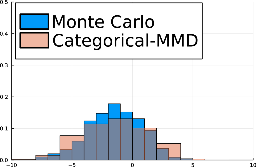
As a preliminary example, we consider 3-state MDPs with the cumulants r(i)=(1γ)ei,i[3]r(i)=(1-\gamma)e_{i},i\in[3] for eie_{i} the iith basis vector. In this setting, ηπ\eta^{\pi} encodes the distribution over trajectory-wise discounted state occupancies, which was discussed in the recent work of [WFG+24] and called the distributional successor measure (DSM). Particularly, [WFG+24] showed that xLaw(Gxr~)x\mapsto\text{Law}\left(G_{x}^{\top}\tilde{r}\right) for Gxηπ(x)G_{x}\sim\eta^{\pi}(x) is the return distribution function for any scalar reward function r~\tilde{r}. Figure 1 shows that the projected categorical dynamic programming algorithm accurately approximates the distribution over discounted state occupancies as well as distributions over returns on held-out reward functions.

Refer to caption
Refer to captionRefer to caption
Refer to caption
Refer to captionRefer to caption
Figure 1: Distributional SMs and associated predicted return distributions with the categorical (left) and EWP (right) representations. Simplex plots denote the distributional SM. Histograms denote the associated return distributions, predicted from a pair of held-out reward functions.

6 Multivariate Distributional TD-Learning

Next, we devise an algorithm for approximating the multi-return distribution function when the transition kernel and reward function are not known, and are observed only through samples. Indeed, this is a strong motivation for TD-learning algorithms [Sut88], wherein state transition data alone is used to solve the Bellman equation. In this section, we devise a TD-learning algorithm for multivariate DRL, leveraging our results on categorical dynamic programming in MMDκ¯\overline{\mathrm{MMD}_{\kappa}}.

Relaxation to signed measures. In the d=1d=1 setting, the categorical projection presented above is known to be affine [RBD+18], making scalar categorical TD-learning amenable to common techniques in stochastic approximation theory. However, the projection is not affine when d2d\geq 2; we give an explicit example in Appendix D. Thus, we relax the categorical representation to include signed measures, which will provide us with an affine projection [BRCM19]—this is crucial for proving our main result, Theorem 6. We denote by 1(𝒴)\mathcal{M}^{1}(\mathcal{Y}) the set of all signed measures μ\mu over 𝒴\mathcal{Y} with μ(𝒴)=1\mu(\mathcal{Y})=1. We begin by noting that the MMD endows 1(𝒴)\mathcal{M}^{1}(\mathcal{Y}) with a metric structure.

{restatable}

lemmammdsigned Let κ:𝒴×𝒴𝐑\kappa:\mathcal{Y}\times\mathcal{Y}\to\operatorname{\mathbf{R}} be a characteristic kernel over some space 𝒴\mathcal{Y}. Then MMDκ:1(𝒴)×1(𝒴)𝐑+\mathrm{MMD}_{\kappa}:\mathcal{M}^{1}(\mathcal{Y})\times\mathcal{M}^{1}(\mathcal{Y})\to\operatorname{\mathbf{R}}_{+} given by (p,q)μpμq(p,q)\mapsto\|\mu_{p}-\mu_{q}\|_{\mathcal{H}} defines a metric on 1(𝒴)\mathcal{M}^{1}(\mathcal{Y}), where μp\mu_{p} denotes the usual mean embedding of pp and \mathcal{H} is the RKHS with kernel κ\kappa.

We define the relaxed projection ΠSC,κ:1([0,(1γ)1Rmax]d)𝒳x𝒳1((x))=:𝒮\Pi_{\mathrm{SC},\kappa}^{\mathcal{R}}:\mathcal{M}^{1}([0,(1-\gamma)^{-1}R_{\max}]^{d})^{\mathcal{X}}\to\prod_{x\in\mathcal{X}}\mathcal{M}^{1}(\mathcal{R}(x))=:\mathscr{S}_{\mathcal{R}},

(ΠSC,κη)(x)arginfp1((x))MMDκ(p,η(x)).\left(\Pi_{\mathrm{SC},\kappa}^{\mathcal{R}}\eta\right)(x)\in\operatorname*{arginf}_{p\in\mathcal{M}^{1}(\mathcal{R}(x))}\mathrm{MMD}_{\kappa}(p,\eta(x)). (10)

Note that (10)\eqref{eq:catproj:sm} is very similar to the definition of the categorical MMD projection in (7)—the only difference is that the optimization occurs over the larger class of signed mass-1 measures. It is also worth noting that the distributional Bellman operator can be applied directly to signed measures, which yields the following convenient result.

{restatable}

lemmasmprojlikecatproj Under the conditions of Corollary 1, the projected operator ΠSC,κ𝒯π:𝒮𝒮\Pi_{\mathrm{SC},\kappa}^{\mathcal{R}}\mathcal{T}^{\pi}:\mathscr{S}_{\mathcal{R}}\to\mathscr{S}_{\mathcal{R}} is affine, is contractive with contraction factor γc/2\gamma^{c/2}, and has a unique fixed point ηSC,κπ\eta_{\mathrm{SC},\kappa}^{\pi}.

While we have “relaxed” the projection, the fixed point ηSC,κπ\eta_{\mathrm{SC},\kappa}^{\pi} is a good approximation of ηπ\eta^{\pi}.

{restatable}

theoremsmqualityfixedpoint Under the conditions of Lemma 6, we have that

  1. 1.

    MMDκ¯(ηSC,κπ,ηπ)11γc/2supx𝒳infP𝒫(x)𝗆𝖾𝗌𝗁(P;κ)\overline{\mathrm{MMD}_{\kappa}}(\eta_{\mathrm{SC},\kappa}^{\pi},\eta^{\pi})\leq\frac{1}{1-\gamma^{c/2}}\sup_{x\in\mathcal{X}}\inf_{P\in\mathscr{P}_{\mathcal{R}(x)}}\sqrt{\mathsf{mesh}(P;\kappa)}; and

  2. 2.

    MMDκ¯(ΠC,κηSC,κπ,ηπ)(1+11γc/2)supx𝒳infP𝒫(x)𝗆𝖾𝗌𝗁(P;κ)\overline{\mathrm{MMD}_{\kappa}}(\Pi_{\mathrm{C},\kappa}^{\mathcal{R}}\eta_{\mathrm{SC},\kappa}^{\pi},\eta^{\pi})\leq(1+\frac{1}{1-\gamma^{c/2}})\sup_{x\in\mathcal{X}}\inf_{P\in\mathscr{P}_{\mathcal{R}(x)}}\sqrt{\mathsf{mesh}(P;\kappa)}.

Notably, the second statement of Theorem 6 states that projecting ηSC,κπ\eta_{\mathrm{SC},\kappa}^{\pi} back onto the space of multi-return distribution functions yields approximately the same error as ηC,κπ\eta_{\mathrm{C},\kappa}^{\pi} when γ\gamma is near 11.

In the remainder of the section, we assume access to a stream of MDP transitions {Tt}t=1𝒳×𝒜×𝐑d×𝒳\left\{{T}_{t}\right\}_{t=1}^{\infty}\subset\mathcal{X}\times\mathcal{A}\times\operatorname{\mathbf{R}}^{d}\times\mathcal{X} consisting of elements Tt=(Xt,At,Rt,Xt)T_{t}=(X_{t},A_{t},R_{t},X^{\prime}_{t}) with the following structure,

Xt𝐏(t1)Atπ(Xt)Rt=r(Xt)XtP(Xt,At)X_{t}\sim\mathbf{P}(\cdot\mid\mathcal{F}_{t-1})\qquad A_{t}\sim\pi(\cdot\mid X_{t})\qquad R_{t}=r(X_{t})\qquad X^{\prime}_{t}\sim P(\cdot\mid X_{t},A_{t}) (11)

where 𝐏\mathbf{P} is some probability measure and {t}t=1\left\{{\mathcal{F}}_{t}\right\}_{t=1}^{\infty} is the canonical filtration t=σ(t=1tTt)\mathcal{F}_{t}=\sigma(\cup_{t=1}^{t}T_{t}). Based on these transitions, we can define stochastic distributional Bellman backups by

𝒯^tπη(x)={(bRt,γ)η(Xt)x=Xtη(x)otherwise,\widehat{\mathcal{T}}^{\pi}_{t}\eta(x)=\begin{cases}(\mathrm{b}_{R_{t},\gamma})_{\sharp}\eta(X_{t}^{\prime})&x=X_{t}\\ \eta(x)&\text{otherwise}\end{cases}, (12)

which notably can be computed exactly without knowledge of P,rP,r. Due to the stronger convergence guarantees shown for projected multivariate distributional dynamic programming, we introduce an asynchronous incremental algorithm leveraging the categorical representation, which produces iterates {η^t}t=1\left\{{\widehat{\eta}}_{t}\right\}_{t=1}^{\infty} according to

η^t+1=(1αt)η^t+αtΠSC,κ𝒯^tπη^t\widehat{\eta}_{t+1}=(1-\alpha_{t})\widehat{\eta}_{t}+\alpha_{t}\Pi_{\mathrm{SC},\kappa}^{\mathcal{R}}\widehat{\mathcal{T}}^{\pi}_{t}\widehat{\eta}_{t} (13)

for η^0𝒞\widehat{\eta}_{0}\in\mathscr{C}_{\mathcal{R}}, where {αt}t=1\left\{{\alpha}_{t}\right\}_{t=1}^{\infty} is any sequence of (possibly) random step sizes adapted to the filtration {t}t=1\left\{{\mathcal{F}}_{t}\right\}_{t=1}^{\infty}. The iterates of (13) closely resemble those of classic stochastic approximation algorithms [RM51] and particularly asynchronous TD learning algorithms [JJS93, Tsi94, BT96], but with iterates taking values in the space of state-indexed signed measures. Indeed, our next result draws on the techniques from these works to establish convergence of TD-learning on 𝒮\mathscr{S}_{\mathcal{R}} representations.

{restatable}

theoremcattdconvergence For a kernel κ\kappa induced by a semimetric ρ\rho of strong negative type, the sequence {η^t}t=1\left\{{\widehat{\eta}}_{t}\right\}_{t=1}^{\infty} given by (11)-(13) converges to ηSC,κπ\eta_{\mathrm{SC},\kappa}^{\pi} with probability 1.

6.1 Simulations: Distributional Successor Features

Refer to caption
Figure 2: Accuracy of zero-shot return distributions over random MDPs, d=2d=2, 95% CI.

To illustrate the behavior of our categorical TD algorithm, we employ it to learn the multi-return distributions for several tabular MDPs with random cumulants. We focus on the case of 22- and 33-dimensional cumulants, which is the setting studied in recent works regarding multivariate distributional RL [ZCZ+21, WUS23]. Interpreting the multi-return distributions as joint distributions over successor features [BDM+18, SFs], we additionally evaluate the return distributions for random reward functions in the span of the cumulants. We compare our categorical TD approach with a tabular implementation of the EWP TD algorithm of [ZCZ+21], for which no convergence bounds are known.

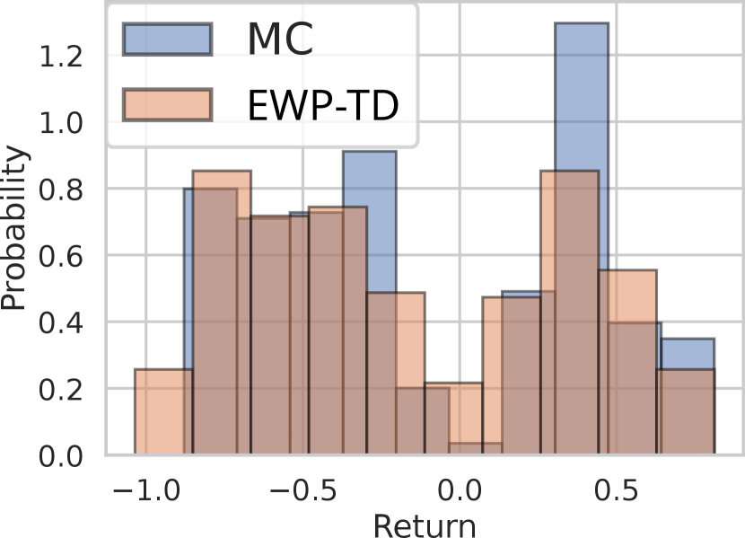
Figure 2 compares TD learning approaches based on their ability to accurately infer (scalar) return distributions on held out reward functions, averaged over 100 random MDPs, with transitions drawn from Dirichlet priors and 22-dimensional cumulants drawn from uniform priors. The performance of the categorical algorithms sharply increases as the number of atoms increases. On the other hand, the EWP TD algorithm performs well with few atoms, but does not improve very much with higher-resolution representations. We posit this is due to the algorithm getting stuck in local minima, given the non-convexity of the EWP MMD objective. This hypothesis is supported as well by Figure 4, which depicts the learned distributional SFs and return distribution predictions.

Refer to caption
Figure 3: Accuracy of zero-shot return distributions over random MDPs, d=3d=3, 95% CI.

Particularly, we observe that the learned particle locations in the EWP TD approach tend to cluster in some areas or get stuck in low-density regimes, which suggests the presence of a local optimum. On the other hand, our provably-convergent categorical TD method learns a high fidelity quantization of the true multi-return distributions.

Naturally, however, the benefits of the 𝗉𝗈𝗅𝗒(d)\mathsf{poly}(d) bounds for EWP suggested by Theorem 4 become more present as we increase the cumulant dimension. Figure 3 repeats the experiment of Figure 2 with d=3d=3, using randomized support points for the categorical algorithm to avoid a cubic growth in the cardinality of the supports. Notably, our method is the first capable of supporting such unstructured supports. While the categorical TD approach can still outperform EWP, a much larger number of atoms is required. This is unsurprising in light of our theoretical results.

Refer to caption
Refer to captionRefer to caption
Refer to caption
Refer to captionRefer to caption
Figure 4: Distributional SFs and predicted return distributions with m=400m=400 atoms, in a random MDP with known rectangular bound on cumulants. Left: Categorical TD. Right: EWP TD.

7 Conclusion

We have provided the first provably convergent and computationally tractable algorithms for learning multivariate return distributions in tabular MDPs. Our theoretical results include convergence guarantees that indicate how accuracy scales with the number of particles mm used in distribution representations, and interestingly motivate the use of signed measures to develop provably convergent TD algorithms.

While it is difficult to scale categorical representations to high-dimensional cumulants, our algorithm is highly performant in the low dd setting, which has been the focus of recent work in multivariate distributional RL. Notably, even the d=2d=2 setting has important applications—indeed, efforts in safe RL depend on distinguishing a cost signal from a reward signal (see, e.g., [YSTS23]), which can be modeled by bivariate distributional RL. In this setting, our method can easily be scaled to large state spaces by approximating the categorical signed measures with neural networks; an illustrated example is given in Appendix F.

On the other hand, the prospect of learning multi-return distributions for high-dimensional cumulants also has many important applications, such as modeling close approximations to distributional successor measures [WFG+24] for zero-shot risk-sensitive policy evaluation. In this setting, we believe EWP-based multivariate DRL will be highly impactful. Our results concerning EWP dynamic programming provide promising evidence that the accuracy of EWP representations scales gracefully with dd for a fixed number of atoms. Thus, we believe that understanding convergence of EWP TD-learning algorithms is a very interesting and important open problem for future investigation.

Acknowledgements

The authors would like to thank Yunhao Tang, Tyler Kastner, Arnav Jain, Yash Jhaveri, Will Dabney, David Meger, and Marc Bellemare for their helpful feedback, as well as insightful suggestions from anonymous reviewers. This work was supported by the Fonds de Recherche du Québec, the National Sciences and Engineering Research Council of Canada, and the compute resources provided by Mila (mila.quebec).

References

  • [BB96] Steven J. Bradtke and Andrew G. Barto. Linear least-squares algorithms for temporal difference learning. Machine Learning, 22(1):33–57, 1996.
  • [BBC+21] Mathieu Blondel, Quentin Berthet, Marco Cuturi, Roy Frostig, Stephan Hoyer, Felipe Llinares-López, Fabian Pedregosa, and Jean-Philippe Vert. Efficient and modular implicit differentiation. In Advances in Neural Information Processing Systems, 2021.
  • [BCC+20] Marc G. Bellemare, Salvatore Candido, Pablo Samuel Castro, Jun Gong, Marlos C. Machado, Subhodeep Moitra, Sameera S. Ponda, and Ziyu Wang. Autonomous navigation of stratospheric balloons using reinforcement learning. Nature, 588(7836):77–82, December 2020.
  • [BDM+17a] André Barreto, Will Dabney, Rémi Munos, Jonathan J. Hunt, Tom Schaul, Hado P. van Hasselt, and David Silver. Successor features for transfer in reinforcement learning. In Advances in Neural Information Processing Systems, 2017.
  • [BDM17b] Marc G. Bellemare, Will Dabney, and Rémi Munos. A Distributional Perspective on Reinforcement Learning. In Proceedings of the International Conference on Machine Learning, 2017.
  • [BDM+18] André Barreto, Will Dabney, Rémi Munos, Jonathan J. Hunt, Tom Schaul, Hado van Hasselt, and David Silver. Successor Features for Transfer in Reinforcement Learning, April 2018.
  • [BDR23] Marc G. Bellemare, Will Dabney, and Mark Rowland. Distributional Reinforcement Learning. The MIT Press, 2023.
  • [BEKS17] Jeff Bezanson, Alan Edelman, Stefan Karpinski, and Viral B. Shah. Julia: A fresh approach to numerical computing. SIAM Review, 59(1):65–98, 2017.
  • [BFH+18] James Bradbury, Roy Frostig, Peter Hawkins, Matthew James Johnson, Chris Leary, Dougal Maclaurin, George Necula, Adam Paszke, Jake VanderPlas, Skye Wanderman-Milne, and Qiao Zhang. JAX: composable transformations of Python+NumPy programs, 2018.
  • [BHB+20] André Barreto, Shaobo Hou, Diana Borsa, David Silver, and Doina Precup. Fast reinforcement learning with generalized policy updates. Proceedings of the National Academy of Sciences (PNAS), 117(48):30079–30087, 2020.
  • [BRCM19] Marc G Bellemare, Nicolas Le Roux, Pablo Samuel Castro, and Subhodeep Moitra. Distributional reinforcement learning with linear function approximation. In Proceedings of the International Conference on Artificial Intelligence and Statistics, 2019.
  • [BT96] Dimitri P. Bertsekas and John N. Tsitsiklis. Neuro-dynamic programming. Athena Scientific, 1996.
  • [CGH+96] Robert M. Corless, Gaston H. Gonnet, David E.G. Hare, David J. Jeffrey, and Donald E. Knuth. On the Lambert W function. Advances in Computational Mathematics, 5:329–359, 1996.
  • [CZZ+24] Xin-Qiang Cai, Pushi Zhang, Li Zhao, Jiang Bian, Masashi Sugiyama, and Ashley Llorens. Distributional Pareto-optimal multi-objective reinforcement learning. In Advances in Neural Information Processing Systems, 2024.
  • [DKNU+20] Will Dabney, Zeb Kurth-Nelson, Naoshige Uchida, Clara Kwon Starkweather, Demis Hassabis, Rémi Munos, and Matthew Botvinick. A distributional code for value in dopamine-based reinforcement learning. Nature, 577(7792):671–675, 2020.
  • [DRBM18] Will Dabney, Mark Rowland, Marc G. Bellemare, and Rémi Munos. Distributional Reinforcement Learning with Quantile Regression. In Proceedings of the AAAI Conference on Artificial Intelligence, 2018.
  • [FSMT19] Dror Freirich, Tzahi Shimkin, Ron Meir, and Aviv Tamar. Distributional Multivariate Policy Evaluation and Exploration with the Bellman GAN. In Proceedings of the International Conference on Machine Learning, 2019.
  • [GBR+12] Arthur Gretton, Karsten M. Borgwardt, Malte J. Rasch, Bernhard Schölkopf, and Alexander Smola. A Kernel Two-Sample Test. Journal of Machine Learning Research, 13(25):723–773, 2012.
  • [GBSL21] Michael Gimelfarb, André Barreto, Scott Sanner, and Chi-Guhn Lee. Risk-Aware Transfer in Reinforcement Learning using Successor Features. In Advances in Neural Information Processing Systems, 2021.
  • [HRB+22] Conor F. Hayes, Roxana Radulescu, Eugenio Bargiacchi, Johan Källström, Matthew Macfarlane, Mathieu Reymond, Timothy Verstraeten, Luisa M. Zintgraf, Richard Dazeley, Fredrik Heintz, Enda Howley, Athirai A. Irissappane, Patrick Mannion, Ann Nowé, Gabriel de Oliveira Ramos, Marcello Restelli, Peter Vamplew, and Diederik M. Roijers. A practical guide to multi-objective reinforcement learning and planning. In Proceedings of the International Conference on Autonomous Agents and Multiagent Systems (AAMAS), 2022.
  • [JJS93] Tommi Jaakkola, Michael I. Jordan, and Satinder P. Singh. On the Convergence of Stochastic Iterative Dynamic Programming Algorithms. In Advances in Neural Information Processing Systems, 1993.
  • [KEF23] Tyler Kastner, Murat A. Erdogdu, and Amir-massoud Farahmand. Distributional Model Equivalence for Risk-Sensitive Reinforcement Learning. In Advances in Neural Information Processing Systems, 2023.
  • [Lax02] Peter D. Lax. Functional analysis. John Wiley & Sons, 2002.
  • [LB22] Alix Lhéritier and Nicolas Bondoux. A Cramér Distance perspective on Quantile Regression based Distributional Reinforcement Learning. In Proceedings of the International Conference on Artificial Intelligence and Statistics, 2022.
  • [LK24] Dong Neuck Lee and Michael R. Kosorok. Off-policy reinforcement learning with high dimensional reward. arXiv preprint arXiv:2408.07660, 2024.
  • [LM22] Shiau Hong Lim and Ilyas Malik. Distributional Reinforcement Learning for Risk-Sensitive Policies. In Advances in Neural Information Processing Systems, 2022.
  • [MSK+10] Tetsuro Morimura, Masashi Sugiyama, Hisashi Kashima, Hirotaka Hachiya, and Toshiyuki Tanaka. Nonparametric return distribution approximation for reinforcement learning. In Proceedings of the International Conference on Machine Learning, 2010.
  • [NGV20] Thanh Tang Nguyen, Sunil Gupta, and Svetha Venkatesh. Distributional Reinforcement Learning via Moment Matching. In AAAI, 2020.
  • [RBD+18] Mark Rowland, Marc G. Bellemare, Will Dabney, Remi Munos, and Yee Whye Teh. An Analysis of Categorical Distributional Reinforcement Learning. In Proceedings of the International Conference on Artificial Intelligence and Statistics, 2018.
  • [RM51] Herbert Robbins and Sutton Monro. A Stochastic Approximation Method. The Annals of Mathematical Statistics, 22(3):400–407, September 1951.
  • [RMA+23] Mark Rowland, Rémi Munos, Mohammad Gheshlaghi Azar, Yunhao Tang, Georg Ostrovski, Anna Harutyunyan, Karl Tuyls, Marc G. Bellemare, and Will Dabney. An Analysis of Quantile Temporal-Difference Learning. arXiv, 2023.
  • [ROH+21] Mark Rowland, Shayegan Omidshafiei, Daniel Hennes, Will Dabney, Andrew Jaegle, Paul Muller, Julien Pérolat, and Karl Tuyls. Temporal difference and return optimism in cooperative multi-agent reinforcement learning. In AAMAS ALA Workshop, 2021.
  • [RVWD13] Diederik M. Roijers, Peter Vamplew, Shimon Whiteson, and Richard Dazeley. A survey of multi-objective sequential decision-making. Journal of Artificial Intelligence Research (JAIR), 48:67–113, 2013.
  • [Sch00] Bernhard Schölkopf. The Kernel Trick for Distances. In Advances in Neural Information Processing Systems, 2000.
  • [SFS24] Eiki Shimizu, Kenji Fukumizu, and Dino Sejdinovic. Neural-kernel conditional mean embeddings. arXiv, 2024.
  • [She21] Vladimir Shenmaier. On the Complexity of the Geometric Median Problem with Outliers. arXiv, 2021.
  • [SLL21] Wei-Fang Sun, Cheng-Kuang Lee, and Chun-Yi Lee. DFAC framework: Factorizing the value function via quantile mixture for multi-agent distributional Q-learning. In Proceedings of the International Conference on Machine Learning, 2021.
  • [SR13] Gábor J. Székely and Maria L. Rizzo. Energy statistics: A class of statistics based on distances. Journal of Statistical Planning and Inference, 143(8):1249–1272, August 2013.
  • [SSGF13] Dino Sejdinovic, Bharath Sriperumbudur, Arthur Gretton, and Kenji Fukumizu. Equivalence of distance-based and RKHS-based statistics in hypothesis testing. The Annals of Statistics, 41(5), October 2013.
  • [Sut88] Richard S. Sutton. Learning to predict by the methods of temporal differences. Machine Learning, 3:9–44, 1988.
  • [SZS+08] Le Song, Xinhua Zhang, Alex Smola, Arthur Gretton, and Bernhard Schölkopf. Tailoring density estimation via reproducing kernel moment matching. In Proceedings of the 25th international conference on Machine learning, pages 992–999, 2008.
  • [Tsi94] John N. Tsitsiklis. Asynchronous stochastic approximation and Q-learning. Machine learning, 16:185–202, 1994.
  • [TSM17] Ilya Tolstikhin, Bharath K. Sriperumbudur, and Krikamol Mu. Minimax estimation of kernel mean embeddings. Journal of Machine Learning Research, 18(86):1–47, 2017.
  • [TVR97] J.N. Tsitsiklis and B. Van Roy. An analysis of temporal-difference learning with function approximation. IEEE Transactions on Automatic Control, 42(5):674–690, 1997.
  • [Vil09] Cédric Villani. Optimal transport: Old and new, volume 338. Springer, 2009.
  • [VN02] Jan Van Neerven. Approximating Bochner integrals by Riemann sums. Indagationes Mathematicae, 13(2):197–208, June 2002.
  • [WBK+22] Peter R Wurman, Samuel Barrett, Kenta Kawamoto, James MacGlashan, Kaushik Subramanian, Thomas J Walsh, Roberto Capobianco, Alisa Devlic, Franziska Eckert, Florian Fuchs, et al. Outracing champion gran turismo drivers with deep reinforcement learning. Nature, 602(7896):223–228, 2022.
  • [WFG+24] Harley Wiltzer, Jesse Farebrother, Arthur Gretton, Yunhao Tang, André Barreto, Will Dabney, Marc G. Bellemare, and Mark Rowland. A distributional analogue to the successor representation. In Proceedings of the International Conference on Machine Learning, 2024.
  • [WUS23] Runzhe Wu, Masatoshi Uehara, and Wen Sun. Distributional Offline Policy Evaluation with Predictive Error Guarantees. In Proceedings of the International Conference on Machine Learning, 2023.
  • [YSTS23] Qisong Yang, Thiago D. Simão, Simon H. Tindemans, and Matthijs T. J. Spaan. Safety-constrained reinforcement learning with a distributional safety critic. Machine Learning, 112(3):859–887, 2023.
  • [YZL+19] Derek Yang, Li Zhao, Zichuan Lin, Tao Qin, Jiang Bian, and Tie-Yan Liu. Fully parameterized quantile function for distributional reinforcement learning. Advances in neural information processing systems, 32, 2019.
  • [ZCZ+21] Pushi Zhang, Xiaoyu Chen, Li Zhao, Wei Xiong, Tao Qin, and Tie-Yan Liu. Distributional Reinforcement Learning for Multi-Dimensional Reward Functions. In Advances in Neural Information Processing Systems, 2021.
\startcontents

[sections] \printcontents[sections]l1

Appendix A In-Depth Summary of Related Work

In Sections 1 and 2, we provided a high-level synopsis of the state of existing work in multivariate distributional RL. In this section, we elaborate further.

Analysis techniques. Our results in this paper mostly drawn on the analysis of one-dimensional distributional RL algorithms such as categorical and quantile dynamic programming, as well as their temporal-difference learning counterparts [RBD+18, DRBM18, RMA+23, BDR23]. The proof techniques in these works themselves are related to contraction-based arguments for reinforcement learning with function approximation [Tsi94, BT96, TVR97].

Multivariate distributional RL algorithms. Several prior works have contributed algorithms for multivariate distributional reinforcement learning, along with empirical demonstrations and theoretical analysis, though as we note in the main paper, the approaches proposed in this paper are the first algorithms with strong theoretical guarantees and efficient tabular implementations. [FSMT19] propose a deep-learning-based approach in which generative adversarial networks are used to model multivariate return distributions, and use these predictions to inform exploration strategies. [ZCZ+21] propose the TD algorithm combing equally-weighted particle representations and an MMD loss that we recall in Equation (3). They demonstrate the effectiveness of this algorithm in combination with deep learning function approximators, though do not analyze it. [WUS23] propose a family of algorithms for multivariate distributional RL termed fitted likelihood evaluation. These methods mirror LSTD algorithms [BB96], iteratively minimising a batch objective function (in this case, a negative log-likelihood, NLL) over a growing dataset. [WUS23] demonstrate that these algorithms are performant in low-dimensional settings empirically, and provide theoretical analysis for FLE algorithms, assuming an oracle which can approximately optimise the NLL objective at each algorithm step. [SFS24] also propose a TD learning algorithm for one-dimensional distributional RL using categorical support and an MMD-based loss. They demonstrate strong performance of this algorithm in classic RL domains such as CartPole and Mountain Car, but do not analyze the algorithm. Our analysis in this paper suggests our novel relaxation to mass-1 signed measures may be crucial to obtaining a straightforwardly analyzable TD algorithm.

Finally, the concurrent work of [LK24] studied distributional Bellman operators for Banach-space-valued reward functions. Their work focuses on analyzing how well the fixed point of a distributional finite-dimensional multivariate Bellman equation can approximate the fixed point of a distributional Banach-space-valued Bellman equation. In contrast, our work only studies finite-dimensional reward functions, but provides explicit convergence rates and approximation bounds when the distribution representations are finite dimensional, unlike [LK24]. Moreover, [LK24] considers a similar algorithm to that discussed in Theorem 4 but for categorical representations, though its convergence is not proved. Furthermore, [LK24] did not prove convergence of any TD-learning algorithms, although they did propose some TD-learning algorithms which achieved interesting results in simulation.

Appendix B Proofs

B.1 Multivariate Distributional Dynamic Programming: Section 3

In this section, we will state some lemmas building up to the proof of Theorem 3. These lemmas generalize corresponding results of [NGV20] that were specific to the scalar reward setting. We begin with a lemma that demonstrates a notion of convexity for the MMD induced by a conditional positive definite kernel.

Lemma 1.

Let (pa)a𝒫(𝒴)(p_{a})_{a\in\mathcal{I}}\subset\mathcal{P}(\mathcal{Y}) and (qa)a𝒫(𝒴)(q_{a})_{a\in\mathcal{I}}\subset\mathcal{P}(\mathcal{Y}) be collections of probability measures indexed by an index set \mathcal{I}. Suppose T𝒫()T\in\mathcal{P}(\mathcal{I}). Then for any characteristic kernel κ\kappa, the following holds,

MMDκ(𝐄aT[pa],𝐄aT[qa])supaMMDκ(pa,qa)\displaystyle\mathrm{MMD}_{\kappa}(\mathbf{E}_{a\sim T}\left[p_{a}\right],\mathbf{E}_{a^{\prime}\sim T}\left[q_{a^{\prime}}\right])\leq\sup_{a\in\mathcal{I}}\mathrm{MMD}_{\kappa}(p_{a},q_{a})
Proof.

It is known from [Sch00] that characteristic kernels generate RKHSs \mathcal{H} into which probability measures can be embedded. As such, it holds that

MMDκ(p,q)=μpμq\displaystyle\mathrm{MMD}_{\kappa}(p,q)=\|\mu_{p}-\mu_{q}\|

where \|\cdot\| is the norm in the Hilbert space \mathcal{H} and μp\mu_{p} is the mean embedding of pp – that is, the unique element of \mathcal{H} such that 𝐄yp[f(y)]=f,μp\mathbf{E}_{y\sim p}\left[f(y)\right]=\langle f,\mu_{p}\rangle for every ff\in\mathcal{H}, and where ,\langle\cdot,\cdot\rangle is the inner product in \mathcal{H}.

Let Tp𝐄aT[pa]T_{p}\triangleq\mathbf{E}_{a\sim T}\left[p_{a}\right] and define TqT_{q} analogously. We claim that μTp=𝐄aT[μpa]Tμp\mu_{Tp}=\mathbf{E}_{a\sim T}\left[\mu_{p_{a}}\right]\triangleq T\mu_{p}. To see this, let ff\in\mathcal{H}, and observe that

𝐄yTp[f](y)\displaystyle\underset{y\sim Tp}{\mathbf{E}}\left[f\right](y) =f(y)Tp(dy)\displaystyle=\int f(y)Tp(\mathrm{d}y)
=f(y)T(da)pa(dy)\displaystyle=\iint f(y)T(\mathrm{d}a)p_{a}(\mathrm{d}y)
=f(y)pa(dy)T(da)\displaystyle=\iint f(y)p_{a}(\mathrm{d}y)T(\mathrm{d}a)
=f,μpaT(da)\displaystyle=\int\langle f,\mu_{p_{a}}\rangle T(\mathrm{d}a)
=f,μpaT(da)\displaystyle=\left\langle f,\int\mu_{p_{a}}T(\mathrm{d}a)\right\rangle
=f,Tμp,\displaystyle=\langle f,T\mu_{p}\rangle,

where the third step invokes Fubini’s theorem, and the penultimate steps leverages the linearity of the inner product. Notably, TT acts as a linear operator on mean embeddings. As a result, we see that

MMDκ(Tp,Tq)\displaystyle\mathrm{MMD}_{\kappa}(Tp,Tq) =μTpμTq\displaystyle=\|\mu_{Tp}-\mu_{Tq}\|
=TμpTμq\displaystyle=\|T\mu_{p}-T\mu_{q}\|
=(μpaμqa)T(da)\displaystyle=\left\|\int_{\mathcal{I}}(\mu_{p_{a}}-\mu_{q_{a}})T(\mathrm{d}a)\right\|
μpaμqaT(da)\displaystyle\leq\int\|\mu_{p_{a}}-\mu_{q_{a}}\|T(\mathrm{d}a)
supaμpaμqa\displaystyle\leq\sup_{a\in\mathcal{I}}\|\mu_{p_{a}}-\mu_{q_{a}}\|
=supaMMDκ(μpa,μqa).\displaystyle=\sup_{a\in\mathcal{I}}\mathrm{MMD}_{\kappa}(\mu_{p_{a}},\mu_{q_{a}}).

where the penultimate inequality is due to Jensen’s inequality, and the final inequality holds since supaμpaμqa\sup_{a\in\mathcal{I}}\|\mu_{p_{a}}-\mu_{q_{a}}\| upper bounds the integrand, and the integral is a monotone operator. ∎

Next, we show how the MMDκ\mathrm{MMD}_{\kappa} under the kernels hypothesized in Theorem 3 behave under affine transformations to random variables.

Lemma 2.

Let κ\kappa be a kernel induced by a semimetric ρ\rho of strong negative type defined over a compact subset 𝒴𝐑d\mathcal{Y}\subset\operatorname{\mathbf{R}}^{d} that is both shift invariant and cc-homogeneous (cf. Theorem 3). Then for any a𝒴a\in\mathcal{Y} and p,q𝒫(𝒴)p,q\in\mathcal{P}(\mathcal{Y}),

MMDκ((ba,γ)p,(ba,γ)q)γc/2MMDκ(p,q).\displaystyle\mathrm{MMD}_{\kappa}((\mathrm{b}_{a,\gamma})_{\sharp}p,(\mathrm{b}_{a,\gamma})_{\sharp}q)\leq\gamma^{c/2}\mathrm{MMD}_{\kappa}(p,q).
Proof.

It is known [GBR+12] that the MMD can be expressed in terms of expected kernel evaluations, according to

MMDκ2(p,q)\displaystyle\mathrm{MMD}_{\kappa}^{2}(p,q) =𝐄[κ(Y,Y)]+𝐄[κ(Z,Z)]2𝐄[κ(Y,Z)]\displaystyle=\underset{}{\mathbf{E}}\left[\kappa(Y,Y^{\prime})\right]+\underset{}{\mathbf{E}}\left[\kappa(Z,Z^{\prime})\right]-2\underset{}{\mathbf{E}}\left[\kappa(Y,Z)\right] (Y,Y,Z,Z)ppqq\displaystyle(Y,Y^{\prime},Z,Z^{\prime})\sim p\otimes p\otimes q\otimes q
=𝐄[12(ρ(Y,y0)+ρ(Y,y0)ρ(Y,Y))]\displaystyle=\underset{}{\mathbf{E}}\left[\frac{1}{2}(\rho(Y,y_{0})+\rho(Y^{\prime},y_{0})-\rho(Y,Y^{\prime}))\right]
+𝐄[12(ρ(Z,y0)+ρ(Z,y0)ρ(Z,Z))]\displaystyle\qquad+\underset{}{\mathbf{E}}\left[\frac{1}{2}(\rho(Z,y_{0})+\rho(Z^{\prime},y_{0})-\rho(Z,Z^{\prime}))\right]
𝐄[ρ(Y,y0)+ρ(Z,y0)ρ(Y,Z)]\displaystyle\qquad-\underset{}{\mathbf{E}}\left[\rho(Y,y_{0})+\rho(Z,y_{0})-\rho(Y,Z)\right]
=𝐄[ρ(Y,Z)]12(𝐄[ρ(Y,Y)]+𝐄[ρ(Z,Z)]),\displaystyle=\underset{}{\mathbf{E}}\left[\rho(Y,Z)\right]-\frac{1}{2}\left(\underset{}{\mathbf{E}}\left[\rho(Y,Y^{\prime})\right]+\underset{}{\mathbf{E}}\left[\rho(Z,Z^{\prime})\right]\right),

where the last step invokes the definition of a kernel induced by a semimetric, and the linearity of expectation. Then, defining Y~,Y~\tilde{Y},\tilde{Y}^{\prime} as independent samples from (ba,γ)p(\mathrm{b}_{a,\gamma})_{\sharp}p and Z~,Z~\tilde{Z},\tilde{Z}^{\prime} as independent samples from (ba,γ)q(\mathrm{b}_{a,\gamma})_{\sharp}q, we have

MMDκ2((ba,γ)p,(ba,γ)q)\displaystyle\mathrm{MMD}_{\kappa}^{2}((\mathrm{b}_{a,\gamma})_{\sharp}p,(\mathrm{b}_{a,\gamma})_{\sharp}q) =𝐄[ρ(Y~,Z~)]12(𝐄[ρ(Y~,Y~)]+𝐄[ρ(Z~,Z~)])\displaystyle=\underset{}{\mathbf{E}}\left[\rho(\tilde{Y},\tilde{Z})\right]-\frac{1}{2}\left(\underset{}{\mathbf{E}}\left[\rho(\tilde{Y},\tilde{Y}^{\prime})\right]+\underset{}{\mathbf{E}}\left[\rho(\tilde{Z},\tilde{Z}^{\prime})\right]\right)
=𝐄[ρ(a+γY,a+γZ)]12(𝐄[ρ(a+γY,a+γY)]+𝐄[ρ(a+γZ,a+γZ)])\displaystyle=\underset{}{\mathbf{E}}\left[\rho(a+\gamma Y,a+\gamma Z)\right]-\frac{1}{2}\left(\underset{}{\mathbf{E}}\left[\rho(a+\gamma Y,a+\gamma Y^{\prime})\right]+\underset{}{\mathbf{E}}\left[\rho(a+\gamma Z,a+\gamma Z^{\prime})\right]\right)
=𝐄[ρ(γY,γZ)]12(𝐄[ρ(γY,γY)]+𝐄[ρ(γZ,γZ)])\displaystyle=\underset{}{\mathbf{E}}\left[\rho(\gamma Y,\gamma Z)\right]-\frac{1}{2}\left(\underset{}{\mathbf{E}}\left[\rho(\gamma Y,\gamma Y^{\prime})\right]+\underset{}{\mathbf{E}}\left[\rho(\gamma Z,\gamma Z^{\prime})\right]\right)
=γc𝐄[ρ(Y,Z)]γc2(𝐄[ρ(Y,Y)]+𝐄[ρ(Z,Z)])\displaystyle=\gamma^{c}\underset{}{\mathbf{E}}\left[\rho(Y,Z)\right]-\frac{\gamma^{c}}{2}\left(\underset{}{\mathbf{E}}\left[\rho(Y,Y^{\prime})\right]+\underset{}{\mathbf{E}}\left[\rho(Z,Z^{\prime})\right]\right)
=γcMMDκ2(p,q),\displaystyle=\gamma^{c}\mathrm{MMD}_{\kappa}^{2}(p,q),

where the second step is a change of variables, the third step invokes the shift invariance of ρ\rho, and the fourth step invokes the homogeneity of ρ\rho.

Thus, it follows that MMDκ((ba,γ)p,(ba,γ)q)γc/2MMDκ(p,q)\mathrm{MMD}_{\kappa}((\mathrm{b}_{a,\gamma})_{\sharp}p,(\mathrm{b}_{a,\gamma})_{\sharp}q)\leq\gamma^{c/2}\mathrm{MMD}_{\kappa}(p,q). ∎

We are now ready to prove the main result of this section.

\dpmmd

*

Proof.

We begin by showing that the distributional Bellman operator 𝒯π\mathcal{T}^{\pi} is contractive in MMDκ¯\overline{\mathrm{MMD}_{\kappa}}. We have

MMDκ¯(𝒯πη1,𝒯πη2)\displaystyle\overline{\mathrm{MMD}_{\kappa}}(\mathcal{T}^{\pi}\eta_{1},\mathcal{T}^{\pi}\eta_{2}) =supx𝒳MMDκ(𝒯πη1(x),𝒯πη2(x))\displaystyle=\sup_{x\in\mathcal{X}}\mathrm{MMD}_{\kappa}(\mathcal{T}^{\pi}\eta_{1}(x),\mathcal{T}^{\pi}\eta_{2}(x))
=supx𝒳MMDκ(𝐄xPπ(x)[(br(x),γ)η1(x)],𝐄x′′Pπ(x)[(br(x),γ)η2(x′′)]).\displaystyle=\sup_{x\in\mathcal{X}}\mathrm{MMD}_{\kappa}\left(\underset{x^{\prime}\sim P^{\pi}(\cdot\mid x)}{\mathbf{E}}\left[(\mathrm{b}_{r(x),\gamma})_{\sharp}\eta_{1}(x^{\prime})\right],\underset{x^{\prime\prime}\sim P^{\pi}(\cdot\mid x)}{\mathbf{E}}\left[(\mathrm{b}_{r(x),\gamma})_{\sharp}\eta_{2}(x^{\prime\prime})\right]\right).

We apply Lemma 1 with =𝒳\mathcal{I}=\mathcal{X} and T=Pπ(x)T=P^{\pi}(\cdot\mid x), yielding

MMDκ¯(𝒯πη1,𝒯πη2)\displaystyle\overline{\mathrm{MMD}_{\kappa}}(\mathcal{T}^{\pi}\eta_{1},\mathcal{T}^{\pi}\eta_{2}) supx𝒳supx𝒳MMDκ((br(x),γ)η1(x),(br(x),γ)η2(x)).\displaystyle\leq\sup_{x\in\mathcal{X}}\sup_{x^{\prime}\in\mathcal{X}}\mathrm{MMD}_{\kappa}\left((\mathrm{b}_{r(x),\gamma})_{\sharp}\eta_{1}(x^{\prime}),(\mathrm{b}_{r(x),\gamma})_{\sharp}\eta_{2}(x^{\prime})\right).

Next, invoking Lemma 2 with the shift-invariance and cc-homogeneity of κ\kappa, we have

MMDκ¯(𝒯πη1,𝒯πη2)\displaystyle\overline{\mathrm{MMD}_{\kappa}}(\mathcal{T}^{\pi}\eta_{1},\mathcal{T}^{\pi}\eta_{2}) γc/2supx𝒳supx𝒳MMDκ(η1(x),η2(x))\displaystyle\leq\gamma^{c/2}\sup_{x\in\mathcal{X}}\sup_{x^{\prime}\in\mathcal{X}}\mathrm{MMD}_{\kappa}\left(\eta_{1}(x^{\prime}),\eta_{2}(x^{\prime})\right)
=γc/2supx𝒳MMDκ(η1(x),η2(x))\displaystyle=\gamma^{c/2}\sup_{x\in\mathcal{X}}\mathrm{MMD}_{\kappa}\left(\eta_{1}(x),\eta_{2}(x)\right)
=γc/2MMDκ¯(η1,η2).\displaystyle=\gamma^{c/2}\overline{\mathrm{MMD}_{\kappa}}(\eta_{1},\eta_{2}).

It follows that MMDκ¯(ηk+1,ηπ)γc/2MMDκ¯(𝒯πηk,𝒯πηπ)=γc/2MMDκ¯(𝒯πηk,ηπ)\overline{\mathrm{MMD}_{\kappa}}(\eta_{k+1},\eta^{\pi})\leq\gamma^{c/2}\overline{\mathrm{MMD}_{\kappa}}(\mathcal{T}^{\pi}\eta_{k},\mathcal{T}^{\pi}\eta^{\pi})=\gamma^{c/2}\overline{\mathrm{MMD}_{\kappa}}(\mathcal{T}^{\pi}\eta_{k},\eta^{\pi}), since ηπ\eta^{\pi} is a fixed point of 𝒯π\mathcal{T}^{\pi}. Continuing, we see that MMDκ¯(ηk,ηπ)γkc/2MMDκ¯(η0,ηπ)γkc/2CO(γkc/2)o(1)\overline{\mathrm{MMD}_{\kappa}}(\eta_{k},\eta^{\pi})\leq\gamma^{kc/2}\overline{\mathrm{MMD}_{\kappa}}(\eta_{0},\eta^{\pi})\leq\gamma^{kc/2}C\in O(\gamma^{kc/2})\subset o(1). Since MMDκ¯\overline{\mathrm{MMD}_{\kappa}} is a metric on 𝒫([0,(1γ)1Rmax]d)𝒳\mathcal{P}([0,(1-\gamma)^{-1}R_{\max}]^{d})^{\mathcal{X}} for any characteristic kernel κ\kappa, it follows that ηk\eta_{k} approaches ηπ\eta^{\pi} at a geometric rate. ∎

B.2 EWP Dynamic Programming: Section 4

In this section, we provide the proof of Theorem 4. To do so, we prove an abstract, general result, regarding any projection mapping that approximates the argmin MMD projection given in Equation (4).

\dpewp

*

Proof.

Let Δk=MMDκ¯(ηk,ηπ)\Delta_{k}=\overline{\mathrm{MMD}_{\kappa}}(\eta_{k},\eta^{\pi}). Then we have

Δk\displaystyle\Delta_{k} =MMDκ¯(Πκ,m(k)𝒯πηk1,𝒯πηπ)\displaystyle=\overline{\mathrm{MMD}_{\kappa}}(\Pi^{(k)}_{\kappa,m}\mathcal{T}^{\pi}\eta_{k-1},\mathcal{T}^{\pi}\eta^{\pi})
MMDκ¯(Πκ,m(k)𝒯πηk1,𝒯πηk1)+MMDκ¯(𝒯πηk1,𝒯πηπ)\displaystyle\leq\overline{\mathrm{MMD}_{\kappa}}(\Pi^{(k)}_{\kappa,m}\mathcal{T}^{\pi}\eta_{k-1},\mathcal{T}^{\pi}\eta_{k-1})+\overline{\mathrm{MMD}_{\kappa}}(\mathcal{T}^{\pi}\eta_{k-1},\mathcal{T}^{\pi}\eta^{\pi})
f(d,m)+γc/2MMDκ¯(ηk1,ηπ)\displaystyle\leq f(d,m)+\gamma^{c/2}\overline{\mathrm{MMD}_{\kappa}}(\eta_{k-1},\eta^{\pi})
Δk\displaystyle\therefore\Delta_{k} f(d,m)+γc/2Δk1,\displaystyle\leq f(d,m)+\gamma^{c/2}\Delta_{k-1},

where the first step invokes the identity that ηπ\eta^{\pi} is the fixed point of 𝒯π\mathcal{T}^{\pi} (which is well-defined by Theorem 3), the second step leverages the triangle inequality, and the third step follows by the definition of f(d,m)f(d,m) and the contractivity of 𝒯π\mathcal{T}^{\pi} established in Theorem 3. Unrolling the recurrence above, we have

MMDκ¯(ηk,ηπ)=Δk\displaystyle\overline{\mathrm{MMD}_{\kappa}}(\eta_{k},\eta^{\pi})=\Delta_{k} γck/2Δ0+f(d,m)i=0γci/2\displaystyle\leq\gamma^{ck/2}\Delta_{0}+f(d,m)\sum_{i=0}^{\infty}\gamma^{ci/2}
γck/2D+f(d,m)1γc/2.\displaystyle\leq\gamma^{ck/2}D+\frac{f(d,m)}{1-\gamma^{c/2}}.

As such, as kk\to\infty, we have that

limkMMDκ¯(ηk,B¯(ηπ,f(d,m)1γc/2))=0,\displaystyle\lim_{k\to\infty}\overline{\mathrm{MMD}_{\kappa}}\left(\eta_{k},\overline{B}\left(\eta^{\pi},\frac{f(d,m)}{1-\gamma^{c/2}}\right)\right)=0,

proving our claim. ∎

Proposition 4, despite its simplicity, reveals an interesting fact: given a good enough approximate MMD projection Πκ,m\Pi_{\kappa,m} in the sense that f(d,m)f(d,m) decays quickly with mm, the dynamic programming iterates (ηk)k0(\eta_{k})_{k\geq 0} will eventually be contained in a (arbitrarily) small neighborhood of ηπ\eta^{\pi}. The next result provides an example consequence of this abstract result, and establishes that m𝗉𝗈𝗅𝗒(d)m\in\mathsf{poly}(d) is enough for convergence to an arbitrarily small set with projected distributional dynamic programming under the EWP representation.

Finally, we can now prove Theorem 4, which we restate below for convenience. \ewpmmddpconvergence*

Proof.

For each x𝒳x\in\mathcal{X} and k[K]k\in[K], denote by x,k\mathcal{E}_{x,k} the event given by

x,k={MMDκ(𝖡𝗈𝗈𝗍𝖯𝗋𝗈𝗃κ,mπηk(x),𝒯πηk(x))2dα/2Rmaxα(1γ)αm+4dα/2Rmaxαlogδ1(1γ)αm=:f(d,m;δ)},\displaystyle\mathcal{E}_{x,k}=\bigg{\{}\mathrm{MMD}_{\kappa}(\mathsf{BootProj}^{\pi}_{\kappa,m}\eta_{k}(x),\mathcal{T}^{\pi}\eta_{k}(x))\leq\frac{2d^{\alpha/2}R_{\max}^{\alpha}}{(1-\gamma)^{\alpha}\sqrt{m}}+\frac{4d^{\alpha/2}R_{\max}^{\alpha}\log\delta^{\prime-1}}{(1-\gamma)^{\alpha}\sqrt{m}}=:f(d,m;\delta^{\prime})\bigg{\}},

for δ>0\delta^{\prime}>0 a constant to be chosen shortly. Moreover, with =(x,k)𝒳×[K]x,k\mathcal{E}=\cap_{(x,k)\in\mathcal{X}\times[K]}\mathcal{E}_{x,k}, it holds that under \mathcal{E}, MMDκ¯(𝖡𝗈𝗈𝗍𝖯𝗋𝗈𝗃κ,mπηk,𝒯πηk)f(d,m;δ)\overline{\mathrm{MMD}_{\kappa}}(\mathsf{BootProj}^{\pi}_{\kappa,m}\eta_{k},\mathcal{T}^{\pi}\eta_{k})\leq f(d,m;\delta^{\prime}) for all k[K]k\in[K]. Following the proof of Proposition 4, we have that, conditioned on \mathcal{E},

MMDκ¯(ηk,ηπ)\displaystyle\overline{\mathrm{MMD}_{\kappa}}(\eta_{k},\eta^{\pi}) γαk/2D+f(d,m;δ)1γα/2\displaystyle\leq\gamma^{\alpha k/2}D+\frac{f(d,m;\delta^{\prime})}{1-\gamma^{\alpha/2}}
2dα/2Rmaxα(1γ)αm+f(d,m;δ)1γα/2.\displaystyle\leq\frac{2d^{\alpha/2}R_{\max}^{\alpha}}{(1-\gamma)^{\alpha}\sqrt{m}}+\frac{f(d,m;\delta^{\prime})}{1-\gamma^{\alpha/2}}.

Now, by [TSM17, Proposition A.1], event x,k\mathcal{E}_{x,k} holds with probability at least 1δ1-\delta^{\prime}, since each (𝖡𝗈𝗈𝗍𝖯𝗋𝗈𝗃κ,mπηk)(x)(\mathsf{BootProj}^{\pi}_{\kappa,m}\eta_{k})(x) is generated independently by sampling mm independent draws from the distribution 𝒯πηk\mathcal{T}^{\pi}\eta_{k}. Therefore, event \mathcal{E} holds with probability at least 1|𝒳|Kδ1-|\mathcal{X}|K\delta^{\prime}. Choosing δ=δ/(|𝒳|K)\delta^{\prime}=\delta/(|\mathcal{X}|K), we have that, with probability at least 1δ1-\delta,

MMDκ¯(ηK,ηπ)\displaystyle\overline{\mathrm{MMD}_{\kappa}}(\eta_{K},\eta^{\pi}) 2dα/2Rmaxα(1γ)αm+11γα/22dα/2Rmaxα(1γ)αm(1+2log(|𝒳|Kδ1))\displaystyle\leq\frac{2d^{\alpha/2}R_{\max}^{\alpha}}{(1-\gamma)^{\alpha}\sqrt{m}}+\frac{1}{1-\gamma^{\alpha/2}}\frac{2d^{\alpha/2}R_{\max}^{\alpha}}{(1-\gamma)^{\alpha}\sqrt{m}}\left(1+2\log(|\mathcal{X}|K\delta^{-1})\right)
2dα/2Rmaxα(1γ)αm+2dα/2Rmaxα(1γα/2)(1γ)αm(1+2log(|𝒳|(1+logmlogγα)δ1)).\displaystyle\leq\frac{2d^{\alpha/2}R_{\max}^{\alpha}}{(1-\gamma)^{\alpha}\sqrt{m}}+\frac{2d^{\alpha/2}R_{\max}^{\alpha}}{(1-\gamma^{\alpha/2})(1-\gamma)^{\alpha}\sqrt{m}}\left(1+2\log\left(|\mathcal{X}|\left(1+\frac{\log m}{\log\gamma^{-\alpha}}\right)\delta^{-1}\right)\right).

As such, there exist universal constants C0,C1𝐑+C_{0},C_{1}\in\operatorname{\mathbf{R}}_{+} such that

MMDκ¯(ηK,ηπ)\displaystyle\overline{\mathrm{MMD}_{\kappa}}(\eta_{K},\eta^{\pi}) C1dα/2Rmaxα(1γα/2)(1γ)αm(1+2log(|𝒳|(1+logmlogγα)δ1))\displaystyle\leq C_{1}\frac{d^{\alpha/2}R_{\max}^{\alpha}}{(1-\gamma^{\alpha/2})(1-\gamma)^{\alpha}\sqrt{m}}\left(1+2\log\left(|\mathcal{X}|\left(1+\frac{\log m}{\log\gamma^{-\alpha}}\right)\delta^{-1}\right)\right) (14)
C0dα/2Rmaxα(1γα/2)(1γ)αm(log|𝒳|+loglogmlogγα+logδ1)\displaystyle\leq C_{0}\frac{d^{\alpha/2}R_{\max}^{\alpha}}{(1-\gamma^{\alpha/2})(1-\gamma)^{\alpha}\sqrt{m}}\left(\log|\mathcal{X}|+\log\frac{\log m}{\log\gamma^{-\alpha}}+\log\delta^{-1}\right)
=C0dα/2Rmaxα(1γα/2)(1γ)αm(log(|𝒳|δ1logγα)+logm).\displaystyle=C_{0}\frac{d^{\alpha/2}R_{\max}^{\alpha}}{(1-\gamma^{\alpha/2})(1-\gamma)^{\alpha}\sqrt{m}}\left(\log\left(\frac{|\mathcal{X}|\delta^{-1}}{\log\gamma^{-\alpha}}\right)+\log m\right).

\dpewporacle

*

Proof.

Proposition 4 shows that projected EWP dynamic programming converges to a set with radius controlled by the quantity f(d,m)f(d,m) that upper bounds the distance f(d,m)f(d,m) between ηk(x)\eta_{k}(x) and Πκ,m(k)ηk(x)\Pi_{\kappa,m}^{(k)}\eta_{k}(x) at the worst state xx. In the proof of Theorem 4, we saw that with nonzero probability, the randomized projections satisfy f(d,m)6dα/2Rmaxα(1γ)αmf(d,m)\leq\frac{6d^{\alpha/2}R^{\alpha}_{\max}}{(1-\gamma)^{\alpha}\sqrt{m}}. Thus, there exists a projection satisfying this bound. Since the projection ΠEWP,κm\Pi_{\mathrm{EWP},\kappa}^{m} is, by definition, the projection with the smallest possible f(d,m)f(d,m), the claim follows directly by Proposition 4. ∎

B.3 Categorical Dynamic Programming: Section 5

\catprojwelldefined

*

Proof.

Firstly, note that Δ(x)\Delta_{\mathcal{R}(x)} is a bounded, finite-dimensional subspace for each x𝒳x\in\mathcal{X}. Thus, Δ(x)\Delta_{\mathcal{R}(x)} is compact, and by the continuity of the MMD, the infimum in (7) is attained.

Following the technique of [SZS+08], we establish that ΠC,κ\Pi_{\mathrm{C},\kappa}^{\mathcal{R}} can be computed as the solution to a particular quadratic program with convex constraints.

Let K𝐑N(x)×N(x)K\in\operatorname{\mathbf{R}}^{N(x)\times N(x)} denote a matrix where Ki,j=κ(ξ(x)i,ξ(x)j)K_{i,j}=\kappa(\xi(x)_{i},\xi(x)_{j}). Since κ\kappa is a positive definite kernel when κ\kappa is characteristic [GBR+12], it follows that KK is a positive definite matrix. Then, for any ϱ𝒫([0,(1γ)1Rmax]d)\varrho\in\mathcal{P}([0,(1-\gamma)^{-1}R_{\max}]^{d}), we have

arginfpΔ(x)MMDκ(p,ϱ)\displaystyle\operatorname*{arginf}_{p\in\Delta_{\mathcal{R}(x)}}\mathrm{MMD}_{\kappa}(p,\varrho)
=arginfpΔ(x)MMDκ2(p,ϱ)\displaystyle=\operatorname*{arginf}_{p\in\Delta_{\mathcal{R}(x)}}\mathrm{MMD}_{\kappa}^{2}(p,\varrho)
=arginfpΔ(x){i=1N(x)j=1N(x)pipjκ(ξ(x)i,ξ(x)j)2i=1N(x)piκ(ξ(x)i,y)ϱ(dy)b𝐑N(x)+M(κ,,ϱ)}\displaystyle=\operatorname*{arginf}_{p\in\Delta_{\mathcal{R}(x)}}\left\{\sum_{i=1}^{N(x)}\sum_{j=1}^{N(x)}p_{i}p_{j}\kappa(\xi(x)_{i},\xi(x)_{j})-2\sum_{i=1}^{N(x)}p_{i}\overbrace{\int\kappa(\xi(x)_{i},y)\varrho(\mathrm{d}y)}^{b\in\operatorname{\mathbf{R}}^{N(x)}}+M(\kappa,\mathcal{R},\varrho)\right\}
=arginfpΔ(x){pKp2pb},\displaystyle=\operatorname*{arginf}_{p\in\Delta_{\mathcal{R}(x)}}\left\{p^{\top}Kp-2p^{\top}b\right\},

where M(κ,,ϱ)M(\kappa,\mathcal{R},\varrho) is independent of pp, so it does not influence the minimization. Now, since KK is positive definite (by virtue of κ\kappa being characteristic) and Δ(x)\Delta_{\mathcal{R}(x)} is a closed convex subset of 𝐑N(x)\operatorname{\mathbf{R}}^{N(x)}, it is well-known that there is unique optimum, and the infimum above is attained for some pΔ(x)p^{\star}\in\Delta_{\mathcal{R}(x)}. Therefore, ΠC,κ\Pi_{\mathrm{C},\kappa}^{\mathcal{R}} is indeed well-defined, and its range is contained in ΠC,κ\Pi_{\mathrm{C},\kappa}^{\mathcal{R}}, confirming the first two claims. Finally, since ΠC,κ\Pi_{\mathrm{C},\kappa}^{\mathcal{R}} is well-defined and since MMDκ\mathrm{MMD}_{\kappa} is nonnegative and separates points, ΠC,κ\Pi_{\mathrm{C},\kappa}^{\mathcal{R}} must map elements of Δ(x)\Delta_{\mathcal{R}(x)} to themselves – this is because MMDκ(p,p)=0\mathrm{MMD}_{\kappa}(p,p)=0 for the kernels we consider. ∎

\projorthogonal

*

Proof.

Fix any x𝒳x\in\mathcal{X} and denote M(x)={μp:pΔ(x)}M(x)=\{\mu_{p}\in\mathcal{H}:p\in\Delta_{\mathcal{R}(x)}\}, where \mathcal{H} is the RKHS induced by the kernel κ\kappa and μp\mu_{p} denotes the mean embedding of pp in this RKHS. It is simple to verify that pμpp\mapsto\mu_{p} is linear: for any p,q𝒫(𝐑d)p,q\in\mathcal{P}(\operatorname{\mathbf{R}}^{d}) and α,β𝐑\alpha,\beta\in\operatorname{\mathbf{R}}, for all ff\in\mathcal{H} with f=1\|f\|=1 we have

f,μαp+βq=f(y)[αp+βq](dy)\displaystyle\langle f,\mu_{\alpha p+\beta q}\rangle=\int f(y)[\alpha p+\beta q](\mathrm{d}y) =αf(y)p(dy)+βf(y)q(dy)\displaystyle=\alpha\int f(y)p(\mathrm{d}y)+\beta\int f(y)q(\mathrm{d}y)
=a,αμp+βμq,\displaystyle=\langle a,\alpha\mu_{p}+\beta\mu_{q}\rangle,

which implies that μαp+βq=αμp+βμq\mu_{\alpha p+\beta q}=\alpha\mu_{p}+\beta\mu_{q}. As a consequence, M(x)M(x) inherits convexity from Δ(x)\Delta_{\mathcal{R}(x)}.

We claim that M(x)M(x) is closed as a subset of \mathcal{H}. Since pμpp\mapsto\mu_{p} is an injection [GBR+12], by Lemma 7, since there is a unique qΔ(x)q\in\Delta_{\mathcal{R}(x)} minimizing MMDκ(p,q)\mathrm{MMD}_{\kappa}(p,q), there is a unique μqM(x)\mu_{q}\in M(x) attaining the infimum μpμq\|\mu_{p}-\mu_{q}\| over M(x)M(x). Let μM(x)\mu\in\mathcal{H}\setminus M(x). Then there exists μqM(x)\mu_{q}\in M(x) such that μqμ=infνM(x)μν\|\mu_{q}-\mu\|=\inf_{\nu\in M(x)}\|\mu-\nu\|, and since μqμ\mu_{q}\neq\mu, it follows that infνM(x)νμ=ϵ>0\inf_{\nu\in M(x)}\|\nu-\mu\|=\epsilon>0. Since this is true for any μM(x)\mu\not\in M(x), it follows that M(x)\mathcal{H}\setminus M(x) is open, so M(x)M(x) is closed.

We will now show that η(x)ΠC,κη(x)\eta(x)\mapsto\Pi_{\mathrm{C},\kappa}^{\mathcal{R}}\eta(x) is a nonexpansion in \mathcal{H}. Let η1,η2𝒞\eta_{1},\eta_{2}\in\mathscr{C}_{\mathcal{R}}, and denote by μ1(x),μ2(x)\mu_{1}(x),\mu_{2}(x) the mean embeddings of η1(x),η2(x)\eta_{1}(x),\eta_{2}(x). We slightly abuse notation and write ΠC,κμi(x)\Pi_{\mathrm{C},\kappa}^{\mathcal{R}}\mu_{i}(x) to denote the mean embedding of ΠC,κηi(x)\Pi_{\mathrm{C},\kappa}^{\mathcal{R}}\eta_{i}(x). Since M(x)M(x) is convex, for any ι(x)M(x)\iota(x)\in M(x) and λ[0,1]\lambda\in[0,1] we have

MMDκ(η1(x),ΠC,κη1(x))2\displaystyle\mathrm{MMD}_{\kappa}(\eta_{1}(x),\Pi_{\mathrm{C},\kappa}^{\mathcal{R}}\eta_{1}(x))^{2} =μ1(x)ΠC,κμ1(x)2\displaystyle=\|\mu_{1}(x)-\Pi_{\mathrm{C},\kappa}^{\mathcal{R}}\mu_{1}(x)\|^{2}
μ1(x)(λι(x)+(1λ)ΠC,κμ1(x))2\displaystyle\leq\|\mu_{1}(x)-(\lambda\iota(x)+(1-\lambda)\Pi_{\mathrm{C},\kappa}^{\mathcal{R}}\mu_{1}(x))\|^{2}
=μ1(x)ΠC,κμ1(x)λ(ι(x)ΠC,κμ1(x))2.\displaystyle=\|\mu_{1}(x)-\Pi_{\mathrm{C},\kappa}^{\mathcal{R}}\mu_{1}(x)-\lambda(\iota(x)-\Pi_{\mathrm{C},\kappa}^{\mathcal{R}}\mu_{1}(x))\|^{2}.

Now, by expanding the squared norms and taking λ0\lambda\downarrow 0, since M(x)M(x) is closed we have

μ1(x)ΠC,κμ1(x),ι1(x)ΠC,κμ1(x)\displaystyle\langle\mu_{1}(x)-\Pi_{\mathrm{C},\kappa}^{\mathcal{R}}\mu_{1}(x),\iota_{1}(x)-\Pi_{\mathrm{C},\kappa}^{\mathcal{R}}\mu_{1}(x)\rangle 0ι1(x),ι2(x)M(x)\displaystyle\leq 0\qquad\forall\iota_{1}(x),\iota_{2}(x)\in M(x)
ΠC,κμ2(x)μ2(x),ΠC,κμ2(x)ι2(x)\displaystyle\therefore\langle\Pi_{\mathrm{C},\kappa}^{\mathcal{R}}\mu_{2}(x)-\mu_{2}(x),\Pi_{\mathrm{C},\kappa}^{\mathcal{R}}\mu_{2}(x)-\iota_{2}(x)\rangle 0,\displaystyle\leq 0,

where the second inequality follows by applying the same logic to μ2(x)\mu_{2}(x). Choosing ι1(x)=ΠC,κμ2(x),ι2(x)=ΠC,κμ1(x)M(x)\iota_{1}(x)=\Pi_{\mathrm{C},\kappa}^{\mathcal{R}}\mu_{2}(x),\iota_{2}(x)=\Pi_{\mathrm{C},\kappa}^{\mathcal{R}}\mu_{1}(x)\in M(x) and adding these inequalities yields

μ1(x)μ2(x)+(ΠC,κμ2(x)ΠC,κμ1(x)),ΠC,κμ2(x)ΠC,κμ1(x)\displaystyle\langle\mu_{1}(x)-\mu_{2}(x)+(\Pi_{\mathrm{C},\kappa}^{\mathcal{R}}\mu_{2}(x)-\Pi_{\mathrm{C},\kappa}^{\mathcal{R}}\mu_{1}(x)),\Pi_{\mathrm{C},\kappa}^{\mathcal{R}}\mu_{2}(x)-\Pi_{\mathrm{C},\kappa}^{\mathcal{R}}\mu_{1}(x)\rangle 0.\displaystyle\leq 0.

Expanding, we see that

MMDκ(ΠC,κη1(x),ΠC,κη2(x))2\displaystyle\mathrm{MMD}_{\kappa}(\Pi_{\mathrm{C},\kappa}^{\mathcal{R}}\eta_{1}(x),\Pi_{\mathrm{C},\kappa}^{\mathcal{R}}\eta_{2}(x))^{2} =ΠC,κμ2(x)ΠC,κμ1(x)2\displaystyle=\|\Pi_{\mathrm{C},\kappa}^{\mathcal{R}}\mu_{2}(x)-\Pi_{\mathrm{C},\kappa}^{\mathcal{R}}\mu_{1}(x)\|^{2}
μ2(x)μ1(x),ΠC,κμ2(x)ΠC,κμ1(x)\displaystyle\leq\langle\mu_{2}(x)-\mu_{1}(x),\Pi_{\mathrm{C},\kappa}^{\mathcal{R}}\mu_{2}(x)-\Pi_{\mathrm{C},\kappa}^{\mathcal{R}}\mu_{1}(x)\rangle
μ2(x)μ1(x)ΠC,κμ2(x)ΠC,κμ1(x)\displaystyle\leq\|\mu_{2}(x)-\mu_{1}(x)\|\|\Pi_{\mathrm{C},\kappa}^{\mathcal{R}}\mu_{2}(x)-\Pi_{\mathrm{C},\kappa}^{\mathcal{R}}\mu_{1}(x)\|
=MMDκ(η1(x),η2(x))MMDκ(ΠC,κη1(x),ΠC,κη2(x))\displaystyle=\mathrm{MMD}_{\kappa}(\eta_{1}(x),\eta_{2}(x))\mathrm{MMD}_{\kappa}(\Pi_{\mathrm{C},\kappa}^{\mathcal{R}}\eta_{1}(x),\Pi_{\mathrm{C},\kappa}^{\mathcal{R}}\eta_{2}(x))
MMDκ(ΠC,κη1(x),ΠC,κη2(x))\displaystyle\therefore\mathrm{MMD}_{\kappa}(\Pi_{\mathrm{C},\kappa}^{\mathcal{R}}\eta_{1}(x),\Pi_{\mathrm{C},\kappa}^{\mathcal{R}}\eta_{2}(x)) MMDκ(η1(x),η2(x)),\displaystyle\leq\mathrm{MMD}_{\kappa}(\eta_{1}(x),\eta_{2}(x)),

confirming that η(x)ΠC,κη(x)\eta(x)\mapsto\Pi_{\mathrm{C},\kappa}^{\mathcal{R}}\eta(x) is a non-expansion. It follows that

MMDκ¯(ΠC,κη1,ΠC,κη2)\displaystyle\overline{\mathrm{MMD}_{\kappa}}(\Pi_{\mathrm{C},\kappa}^{\mathcal{R}}\eta_{1},\Pi_{\mathrm{C},\kappa}^{\mathcal{R}}\eta_{2}) =supx𝒳MMDκ(η1(x),η2(x))\displaystyle=\sup_{x\in\mathcal{X}}\mathrm{MMD}_{\kappa}(\eta_{1}(x),\eta_{2}(x))
supx𝒳MMDκ(η1(x),η2(x))\displaystyle\leq\sup_{x\in\mathcal{X}}\mathrm{MMD}_{\kappa}(\eta_{1}(x),\eta_{2}(x))
=MMDκ¯(η1,η2).\displaystyle=\overline{\mathrm{MMD}_{\kappa}}(\eta_{1},\eta_{2}).

\dpprojfixedpoint

*

Proof.

Combining Theorem 3 and Lemma 1, we see that

MMDκ¯(ΠC,κ𝒯πη1,ΠC,κ𝒯πη2)MMDκ¯(𝒯πη1,η2)γc/2MMDκ¯(η1,η2)\displaystyle\overline{\mathrm{MMD}_{\kappa}}(\Pi_{\mathrm{C},\kappa}^{\mathcal{R}}\mathcal{T}^{\pi}\eta_{1},\Pi_{\mathrm{C},\kappa}^{\mathcal{R}}\mathcal{T}^{\pi}\eta_{2})\leq\overline{\mathrm{MMD}_{\kappa}}(\mathcal{T}^{\pi}\eta_{1},\eta_{2})\leq\gamma^{c/2}\overline{\mathrm{MMD}_{\kappa}}(\eta_{1},\eta_{2})

for some c>0c>0. Thus, ΠC,κ𝒯π\Pi_{\mathrm{C},\kappa}^{\mathcal{R}}\mathcal{T}^{\pi} is a contraction on (𝒞,MMDκ¯)(\mathscr{C}_{\mathcal{R}},\overline{\mathrm{MMD}_{\kappa}}). If \mathcal{H} is the RKHS induced by κ\kappa, we showed in Lemma 1 that 𝒞\mathscr{C}_{\mathcal{R}} is isometric to a product of closed, convex subsets of \mathcal{H}. Therefore, by the completeness of \mathcal{H}, 𝒞\mathscr{C}_{\mathcal{R}} is isometric to a complete subspace, and consequently 𝒞\mathscr{C}_{\mathcal{R}} is a complete subspace under the metric MMDκ¯\overline{\mathrm{MMD}_{\kappa}}. Invoking the Banach fixed-point theorem, it follows that ΠC,κ𝒯π\Pi_{\mathrm{C},\kappa}^{\mathcal{R}}\mathcal{T}^{\pi} has a unique fixed point ηC,κπ\eta_{\mathrm{C},\kappa}^{\pi}, and ηkηC,κπ\eta_{k}\to\eta_{\mathrm{C},\kappa}^{\pi} geometrically. ∎

B.3.1 Quality of the Categorical Fixed Point

As we saw in our analysis of multivariate DRL with EWP representations, the distance between a distribution and its projection (as a function of m,dm,d) plays a major role in controlling the approximation error in projected distributional dynamic programming. Before proving the main results of this section, we begin by analyzing this quantity by reducing it to the largest distance between points among certain partitions of the space of returns.

\mmdprojapprox

*

Proof.

Our proof proceeds by establishing approximation bounds of Riemann sums to the Bochner integral μp\mu_{p}, similar to [VN02]. Let P𝒫P\in\mathscr{P}_{\mathcal{R}}. Abusing notation to denote by Πpi\Pi p_{i} the probability of the iith atom of the discrete support under Πp\Pi p, we have

MMDκ2(p,Πp)\displaystyle\mathrm{MMD}_{\kappa}^{2}(p,\Pi p) =μΠpμp2\displaystyle=\|\mu_{\Pi p}-\mu_{p}\|^{2}
=κ(,y)Πp(dy)κ(,y)p(dy)2\displaystyle=\left\|\int\kappa(\cdot,y)\Pi p(\mathrm{d}y)-\int\kappa(\cdot,y)p(\mathrm{d}y)\right\|^{2}
=iκ(,zi)Πpiκ(,y)p(dy)2,\displaystyle=\left\|\sum_{i}\kappa(\cdot,z_{i})\Pi p_{i}-\int\kappa(\cdot,y)p(\mathrm{d}y)\right\|^{2},

where ={zi}i=1n\mathcal{R}=\{z_{i}\}_{i=1}^{n} for some n𝐍n\in\mathbf{N}. Since Πp\Pi p optimizes the MMD over all probability vectors in Δ\Delta_{\mathcal{R}}, for qΔq\in\Delta_{\mathcal{R}} with qi=p(θi)q_{i}=p(\theta_{i}) for the iith element of PP, we have

MMDκ2(p,Πp)\displaystyle\mathrm{MMD}_{\kappa}^{2}(p,\Pi p) iκ(,zi)p(θi)κ(,y)p(dy)2\displaystyle\leq\left\|\sum_{i}\kappa(\cdot,z_{i})p(\theta_{i})-\int\kappa(\cdot,y)p(\mathrm{d}y)\right\|^{2}
=iθi(κ(,zi)κ(,y))p(dy)2\displaystyle=\left\|\sum_{i}\int_{\theta_{i}}(\kappa(\cdot,z_{i})-\kappa(\cdot,y))p(\mathrm{d}y)\right\|^{2}
isupy1,y2θiκ(,y1)κ(,y2)p(θi)2\displaystyle\leq\left\|\sum_{i}\sup_{y_{1},y_{2}\in\theta_{i}}\|\kappa(\cdot,y_{1})-\kappa(\cdot,y_{2})\|p(\theta_{i})\right\|^{2}
supθPsupy1,y2θκ(,y1)κ(,y2)2.\displaystyle\leq\sup_{\theta\in P}\sup_{y_{1},y_{2}\in\theta}\|\kappa(\cdot,y_{1})-\kappa(\cdot,y_{2})\|^{2}.

It was shown by [SSGF13] that zκ(,z)z\mapsto\kappa(\cdot,z) is an isometry from (𝐑d,ρ1/2)(\operatorname{\mathbf{R}}^{d},\rho^{1/2}) to \mathcal{H}, where \mathcal{H} is the RKHS induced by κ\kappa. Thus, we have

MMDκ2(p,Πp)\displaystyle\mathrm{MMD}_{\kappa}^{2}(p,\Pi p) supθPsupy1,y2θρ(y1,y2)=𝗆𝖾𝗌𝗁(P;κ).\displaystyle\leq\sup_{\theta\in P}\sup_{y_{1},y_{2}\in\theta}\rho(y_{1},y_{2})=\mathsf{mesh}(P;\kappa).

Since this is true for any partition P𝒫P\in\mathscr{P}_{\mathcal{R}}, the claim follows by taking the infimum over 𝒫\mathscr{P}_{\mathcal{R}}. ∎

We now move on to the main results.

\dpconsistent

*

Proof.

The proof begins in a similar manner to [RBD+18, Proposition 3]. Given that ΠC,κ\Pi_{\mathrm{C},\kappa}^{\mathcal{R}} is a nonexpansion as shown in Lemma 1, we have

MMDκ¯(ηC,κπ,ηπ)\displaystyle\overline{\mathrm{MMD}_{\kappa}}(\eta_{\mathrm{C},\kappa}^{\pi},\eta^{\pi}) =supx𝒳MMDκ(ηC,κπ(x),ηπ(x))\displaystyle=\sup_{x\in\mathcal{X}}\mathrm{MMD}_{\kappa}(\eta_{\mathrm{C},\kappa}^{\pi}(x),\eta^{\pi}(x))
supx𝒳[MMDκ(ηC,κπ(x),ΠC,κηπ(x))+MMDκ(ΠC,κηπ(x),ηπ(x))]\displaystyle\leq\sup_{x\in\mathcal{X}}\left[\mathrm{MMD}_{\kappa}(\eta_{\mathrm{C},\kappa}^{\pi}(x),\Pi_{\mathrm{C},\kappa}^{\mathcal{R}}\eta^{\pi}(x))+\mathrm{MMD}_{\kappa}(\Pi_{\mathrm{C},\kappa}^{\mathcal{R}}\eta^{\pi}(x),\eta^{\pi}(x))\right]
MMDκ¯(ηC,κπ,ΠC,κηπ)+MMDκ¯(ΠC,κηπ,ηπ)\displaystyle\leq\overline{\mathrm{MMD}_{\kappa}}(\eta_{\mathrm{C},\kappa}^{\pi},\Pi_{\mathrm{C},\kappa}^{\mathcal{R}}\eta^{\pi})+\overline{\mathrm{MMD}_{\kappa}}(\Pi_{\mathrm{C},\kappa}^{\mathcal{R}}\eta^{\pi},\eta^{\pi})
=(a)MMDκ¯(ΠC,κ𝒯πηC,κπ,ΠC,κ𝒯πηπ)+MMDκ¯(ΠC,κηπ,ηπ)\displaystyle\overset{(a)}{=}\overline{\mathrm{MMD}_{\kappa}}(\Pi_{\mathrm{C},\kappa}^{\mathcal{R}}\mathcal{T}^{\pi}\eta_{\mathrm{C},\kappa}^{\pi},\Pi_{\mathrm{C},\kappa}^{\mathcal{R}}\mathcal{T}^{\pi}\eta^{\pi})+\overline{\mathrm{MMD}_{\kappa}}(\Pi_{\mathrm{C},\kappa}^{\mathcal{R}}\eta^{\pi},\eta^{\pi})
(b)MMDκ¯(𝒯πηC,κπ,𝒯πηπ)+MMDκ¯(ΠC,κηπ,ηπ)\displaystyle\overset{(b)}{\leq}\overline{\mathrm{MMD}_{\kappa}}(\mathcal{T}^{\pi}\eta_{\mathrm{C},\kappa}^{\pi},\mathcal{T}^{\pi}\eta^{\pi})+\overline{\mathrm{MMD}_{\kappa}}(\Pi_{\mathrm{C},\kappa}^{\mathcal{R}}\eta^{\pi},\eta^{\pi})
(c)γc/2MMDκ¯(ηC,κπ,ηπ)+MMDκ¯(ΠC,κηπ,ηπ)\displaystyle\overset{(c)}{\leq}\gamma^{c/2}\overline{\mathrm{MMD}_{\kappa}}(\eta_{\mathrm{C},\kappa}^{\pi},\eta^{\pi})+\overline{\mathrm{MMD}_{\kappa}}(\Pi_{\mathrm{C},\kappa}^{\mathcal{R}}\eta^{\pi},\eta^{\pi})
MMDκ¯(ηC,κπ,ηπ)\displaystyle\therefore\overline{\mathrm{MMD}_{\kappa}}(\eta_{\mathrm{C},\kappa}^{\pi},\eta^{\pi}) 11γc/2MMDκ¯(ΠC,κηπ,ηπ),\displaystyle\leq\frac{1}{1-\gamma^{c/2}}\overline{\mathrm{MMD}_{\kappa}}(\Pi_{\mathrm{C},\kappa}^{\mathcal{R}}\eta^{\pi},\eta^{\pi}),

where (a)(a) leverages the fact that ηC,κπ\eta_{\mathrm{C},\kappa}^{\pi} is the fixed point of ΠC,κ𝒯π\Pi_{\mathrm{C},\kappa}^{\mathcal{R}}\mathcal{T}^{\pi} and that ηπ\eta^{\pi} is the fixed point of 𝒯π\mathcal{T}^{\pi}, (b)(b) follows since ΠC,κ\Pi_{\mathrm{C},\kappa}^{\mathcal{R}} is a nonexpansion by Lemma 1, and (c)(c) follows by the contractivity of 𝒯π\mathcal{T}^{\pi} established in Theorem 3. Finally, by Lemma 1, we have

MMDκ¯(ηC,κπ,ηπ)11γc/2supx𝒳MMDκ(ΠC,κηπ(x),ηπ(x))11γc/2supx𝒳infP𝒫(x)𝗆𝖾𝗌𝗁(P;κ).\displaystyle\overline{\mathrm{MMD}_{\kappa}}(\eta_{\mathrm{C},\kappa}^{\pi},\eta^{\pi})\leq\frac{1}{1-\gamma^{c/2}}\sup_{x\in\mathcal{X}}\mathrm{MMD}_{\kappa}(\Pi_{\mathrm{C},\kappa}^{\mathcal{R}}\eta^{\pi}(x),\eta^{\pi}(x))\leq\frac{1}{1-\gamma^{c/2}}\sup_{x\in\mathcal{X}}\inf_{P\in\mathscr{P}_{\mathcal{R}(x)}}\sqrt{\mathsf{mesh}(P;\kappa)}.

Finally, we explicitly derive a convergence rate for a particular support map under the energy distance kernels.

\meshcovering

*

Proof.

We begin bounding 𝗆𝖾𝗌𝗁(P;κ)\mathsf{mesh}(P;\kappa). Assume m=ndm=n^{d} for some n𝐍n\in\operatorname{\mathbf{N}}. We consider a partition P¯𝒫Um\overline{P}\subset\mathscr{P}_{U_{m}} consisting of dd-dimensional hypercubes with side length (1γ)1Rmax/(n1)(1-\gamma)^{-1}R_{\max}/(n-1). By definition of UmU_{m}, it is clear that these hypercubes cover [0,(1γ)1Rmax]d[0,(1-\gamma)^{-1}R_{\max}]^{d} and each contain exactly one support point. Now, for each θP¯\theta\in\overline{P}, we have

supy1,y2θρ(y1,y2)\displaystyle\sup_{y_{1},y_{2}\in\theta}\rho(y_{1},y_{2}) y(y+(1γ)1Rmax/(n1)12α\displaystyle\leq\|y-(y+(1-\gamma)^{-1}R_{\max}/(n-1)\vec{1}\|_{2}^{\alpha}

where 1\vec{1} is the vector of all ones, and yy is any element in θ\theta. Expanding, we have

supy1,y2θρ(y1,y2)\displaystyle\sup_{y_{1},y_{2}\in\theta}\rho(y_{1},y_{2}) (1γ)α(i=1d(Rmaxn1)2)α/2\displaystyle\leq(1-\gamma)^{-\alpha}\left(\sum_{i=1}^{d}\left(\frac{R_{\max}}{n-1}\right)^{2}\right)^{\alpha/2}
dα/2Rmaxα(1γ)α(n1)α.\displaystyle\leq\frac{d^{\alpha/2}R_{\max}^{\alpha}}{(1-\gamma)^{\alpha}(n-1)^{\alpha}}.

Since this bound holds for any θP¯\theta\in\overline{P}, invoking Theorem 1 yields

MMDκ¯(ηC,κπ,ηπ)\displaystyle\overline{\mathrm{MMD}_{\kappa}}(\eta_{\mathrm{C},\kappa}^{\pi},\eta^{\pi}) 11γα/2supx𝒳infP𝒫Um𝗆𝖾𝗌𝗁(P;κ)\displaystyle\leq\frac{1}{1-\gamma^{\alpha/2}}\sup_{x\in\mathcal{X}}\inf_{P\in\mathscr{P}_{U_{m}}}\sqrt{\mathsf{mesh}(P;\kappa)}
11γα/2supx𝒳𝗆𝖾𝗌𝗁(P¯;κ)\displaystyle\leq\frac{1}{1-\gamma^{\alpha/2}}\sup_{x\in\mathcal{X}}\sqrt{\mathsf{mesh}(\overline{P};\kappa)}
11γα/2supx𝒳dα/2Rmaxα(1γ)α(n2)α\displaystyle\leq\frac{1}{1-\gamma^{\alpha/2}}\sup_{x\in\mathcal{X}}\sqrt{\frac{d^{\alpha/2}R_{\max}^{\alpha}}{(1-\gamma)^{\alpha}(n-2)^{\alpha}}}
=1(1γα/2)(1γ)α/2dα/4Rmaxα/2(n1)α/2\displaystyle=\frac{1}{(1-\gamma^{\alpha/2})(1-\gamma)^{\alpha/2}}\frac{d^{\alpha/4}R_{\max}^{\alpha/2}}{(n-1)^{\alpha/2}}
=1(1γα/2)(1γ)α/2dα/4Rmaxα/2(m1/d1)α/2.\displaystyle=\frac{1}{(1-\gamma^{\alpha/2})(1-\gamma)^{\alpha/2}}\frac{d^{\alpha/4}R_{\max}^{\alpha/2}}{(m^{1/d}-1)^{\alpha/2}}.

If instead m((n1)d,nd)m\in((n-1)^{d},n^{d}), we omit all but (n1)d(n-1)^{d} of the support points, and achieve

MMDκ¯(ηC,κπ,ηπ)\displaystyle\overline{\mathrm{MMD}_{\kappa}}(\eta_{\mathrm{C},\kappa}^{\pi},\eta^{\pi}) 1(1γα/2)(1γ)α/2dα/4Rmaxα/2(m1/d1)α/2.\displaystyle\leq\frac{1}{(1-\gamma^{\alpha/2})(1-\gamma)^{\alpha/2}}\frac{d^{\alpha/4}R_{\max}^{\alpha/2}}{(\lfloor m^{1/d}\rfloor-1)^{\alpha/2}}.

Alternatively, we may write

MMDκ¯(ηC,κπ,ηπ)\displaystyle\overline{\mathrm{MMD}_{\kappa}}(\eta_{\mathrm{C},\kappa}^{\pi},\eta^{\pi}) 1(1γα/2)(1γ)α/2dα/4Rmaxα/2(m1/d2)α/2.\displaystyle\leq\frac{1}{(1-\gamma^{\alpha/2})(1-\gamma)^{\alpha/2}}\frac{d^{\alpha/4}R_{\max}^{\alpha/2}}{(m^{1/d}-2)^{\alpha/2}}.

B.4 Categorical TD Learning: Section 6

In this section, we prove results leading up to and including the convergence of the categorical TD-learning algorithm over mass-1 signed measures. First, in Section B.4.1, we show that MMDκ\mathrm{MMD}_{\kappa} is in fact a metric on the space of mass-1 signed measures, and establish that the multivariate distributional Bellman operator is contractive under these distribution representations. Subsequently, in Section B.4.2, we analyze the temporal difference learning algorithm leveraging the results from Section B.4.1.

B.4.1 The Signed Measure Relaxation

We begin by establishing that MMDκ\mathrm{MMD}_{\kappa} is a metric on 1(𝒴)\mathcal{M}^{1}(\mathcal{Y}) for spaces 𝒴\mathcal{Y} under which MMDκ\mathrm{MMD}_{\kappa} is a metric on 𝒫(𝒴)\mathcal{P}(\mathcal{Y}). \mmdsigned*

Proof.

Naturally, since MMDκ\mathrm{MMD}_{\kappa} is given by a norm, it is non-negative, symmetric, and satisfies the triangle inequality. We must show that MMDκ(p,q)=0p=q\mathrm{MMD}_{\kappa}(p,q)=0\iff p=q. Firstly, it is clear that MMDκ(p,p)=0\mathrm{MMD}_{\kappa}(p,p)=0 by the positive homogeneity of the norm. It remains to show that MMDκ(p,q)=0p=q\mathrm{MMD}_{\kappa}(p,q)=0\implies p=q.

Let pq1(𝒴)p\neq q\in\mathcal{M}^{1}(\mathcal{Y}). For the sake of contradiction, assume that MMDκ(p,q)=0\mathrm{MMD}_{\kappa}(p,q)=0. We will show that this implies that MMDκ(P,Q)=0\mathrm{MMD}_{\kappa}(P,Q)=0 for a pair of distinct probability measures, which is a contradiction since MMDκ\mathrm{MMD}_{\kappa} with characteristic κ\kappa is known to be a metric on 𝒫(𝒴)\mathcal{P}(\mathcal{Y}).

By the Hahn decomposition theorem, we may write p=p~+p~p=\tilde{p}^{+}-\tilde{p}^{-} for non-negative measures p~+,p~\tilde{p}^{+},\tilde{p}^{-}. Therefore, for some a𝐑+a\in\operatorname{\mathbf{R}}_{+}, we may express

p=(a+1)p+ap\displaystyle p=(a+1)p^{+}-ap^{-}

where p+,p𝒫(𝒴)p^{+},p^{-}\in\mathcal{P}(\mathcal{Y}). Likewise, there exist b𝐑+b\in\operatorname{\mathbf{R}}_{+} and probability measure q+,qq^{+},q^{-} for which q=(b+1)q+bqq=(b+1)q^{+}-bq^{-}. Since MMDκ(p,q)=0\mathrm{MMD}_{\kappa}(p,q)=0 by hypothesis, and by linearity of pμpp\mapsto\mu_{p}, we have

0\displaystyle 0 =μpμq\displaystyle=\|\mu_{p}-\mu_{q}\|_{\mathcal{H}}
=(a+1)μp+aμp+bμq(b+1)μq+\displaystyle=\|(a+1)\mu_{p^{+}}-a\mu_{p^{-}}+b\mu_{q^{-}}-(b+1)\mu_{q^{+}}\|_{\mathcal{H}}
=(a+1)μp++bμq(aμp+(b+1)μq+)\displaystyle=\|(a+1)\mu_{p^{+}}+b\mu_{q^{-}}-(a\mu_{p^{-}}+(b+1)\mu_{q^{+}})\|_{\mathcal{H}}
=(a+b+1)(λμp++(1λ)μq)(λμp+(1λ)μq+),λ=a+1a+b+1,λ=aa+b+1\displaystyle=(a+b+1)\left\|\bigg{(}\lambda\mu_{p^{+}}+(1-\lambda)\mu_{q^{-}}\bigg{)}-\bigg{(}\lambda^{\prime}\mu_{p^{-}}+(1-\lambda^{\prime})\mu_{q^{+}}\bigg{)}\right\|,\ \lambda=\frac{a+1}{a+b+1},\ \lambda^{\prime}=\frac{a}{a+b+1}
:=(a+b+1)μPμQ,\displaystyle:=(a+b+1)\|\mu_{P}-\mu_{Q}\|_{\mathcal{H}},

where P=λp++(1λ)qP=\lambda p^{+}+(1-\lambda)q^{-} and Q=λp+(1λ)q+Q=\lambda^{\prime}p^{-}+(1-\lambda^{\prime})q^{+} are convex combinations of probability measures, and are therefore probability measures themselves. So, we have that

λp+λp\displaystyle\lambda p^{+}-\lambda^{\prime}p^{-} =(1λ)q+(1λ)q\displaystyle=(1-\lambda^{\prime})q^{+}-(1-\lambda)q^{-}
(a+1)λp+ap\displaystyle(a+1)\lambda p^{+}-ap^{-} =(b+1)q+bq\displaystyle=(b+1)q^{+}-bq^{-}
p\displaystyle\therefore p =q,\displaystyle=q,

which contradicts our hypothesis. Therefore, MMDκ(p,q)=0p=q\mathrm{MMD}_{\kappa}(p,q)=0\iff p=q for any p,q1(𝒴)p,q\in\mathcal{M}^{1}(\mathcal{Y}), and it follows that MMDκ\mathrm{MMD}_{\kappa} is a metric. ∎

Next, we show that the distributional Bellman operator is contractive on the space of mass-1 signed measure return distribution representations.

\smprojlikecatproj

*

Proof.

Indeed, ΠSC,κ\Pi_{\mathrm{SC},\kappa}^{\mathcal{R}} is, in a sense, a simpler operator than ΠC,κ\Pi_{\mathrm{C},\kappa}^{\mathcal{R}}. Since 1((x))\mathcal{M}^{1}(\mathcal{R}(x)) is an affine subspace of 1(𝐑d)\mathcal{M}^{1}(\operatorname{\mathbf{R}}^{d}), it holds that ΠSC,κ\Pi_{\mathrm{SC},\kappa}^{\mathcal{R}} is simply a Hilbertian projection, which is known to be affine and a nonexpansion [Lax02]. Moreover, since 𝒯π\mathcal{T}^{\pi} acts identically on 1(𝐑d)\mathcal{M}^{1}(\operatorname{\mathbf{R}}^{d}) as it does on 𝒫(𝐑d)\mathcal{P}(\operatorname{\mathbf{R}}^{d}), it immediately follows that 𝒯π\mathcal{T}^{\pi} is a γc/2\gamma^{c/2}-contraction on 1(𝐑d)\mathcal{M}^{1}(\operatorname{\mathbf{R}}^{d}), inheriting the result from Theorem 3. Thus, we have that for any η1,η2𝒮\eta_{1},\eta_{2}\in\mathscr{S}_{\mathcal{R}},

MMDκ(ΠSC,κ𝒯πη1,ΠSC,κ𝒯πη2)\displaystyle\mathrm{MMD}_{\kappa}(\Pi_{\mathrm{SC},\kappa}^{\mathcal{R}}\mathcal{T}^{\pi}\eta_{1},\Pi_{\mathrm{SC},\kappa}^{\mathcal{R}}\mathcal{T}^{\pi}\eta_{2}) MMDκ(𝒯πη1,𝒯πη2)\displaystyle\leq\mathrm{MMD}_{\kappa}(\mathcal{T}^{\pi}\eta_{1},\mathcal{T}^{\pi}\eta_{2})
γc/2MMDκ(η1,η2)\displaystyle\leq\gamma^{c/2}\mathrm{MMD}_{\kappa}(\eta_{1},\eta_{2})

confirming that the projected operator is a contraction. Since MMDκ\mathrm{MMD}_{\kappa} is a metric on 1((x))\mathcal{M}^{1}(\mathcal{R}(x)) for each x𝒳x\in\mathcal{X}, it follows that MMDκ¯\overline{\mathrm{MMD}_{\kappa}} is a metric on 𝒮\mathscr{S}_{\mathcal{R}}. The existence and uniqueness of the fixed point ηSC,κπ\eta_{\mathrm{SC},\kappa}^{\pi} follows by the Banach fixed point theorem. ∎

Finally, we show that the fixed point of distributional dynamic programming with signed measure representations is roughly as accurate as ηC,κπ\eta_{\mathrm{C},\kappa}^{\pi}.

\smqualityfixedpoint

*

Proof.

Since ΠSC,κ\Pi_{\mathrm{SC},\kappa}^{\mathcal{R}} is a nonexpansion in MMDκ¯\overline{\mathrm{MMD}_{\kappa}} by Lemma 6, following the procedure of Theorem 1, we have

MMDκ¯(ηSC,κπ,ηπ)11γc/2MMDκ¯(ΠSC,κηπ,ηπ).\displaystyle\overline{\mathrm{MMD}_{\kappa}}(\eta_{\mathrm{SC},\kappa}^{\pi},\eta^{\pi})\leq\frac{1}{1-\gamma^{c/2}}\overline{\mathrm{MMD}_{\kappa}}(\Pi_{\mathrm{SC},\kappa}^{\mathcal{R}}\eta^{\pi},\eta^{\pi}).

Note that ΠSC,κηπ\Pi_{\mathrm{SC},\kappa}^{\mathcal{R}}\eta^{\pi} identifies the closest point (in MMDκ¯\overline{\mathrm{MMD}_{\kappa}}) to ηπ\eta^{\pi} in 𝒮:=x𝒳1((x))\mathscr{S}_{\mathcal{R}}:=\prod_{x\in\mathcal{X}}\mathcal{M}^{1}(\mathcal{R}(x)) and ΠC,κηπ\Pi_{\mathrm{C},\kappa}^{\mathcal{R}}\eta^{\pi} identifies the closest point to ηπ\eta^{\pi} in 𝒞:=x𝒳Δ(x)\mathscr{C}_{\mathcal{R}}:=\prod_{x\in\mathcal{X}}\Delta_{\mathcal{R}(x)}. Since it is clear that 𝒞𝒮\mathscr{C}_{\mathcal{R}}\subset\mathscr{S}_{\mathcal{R}}, it follows that

MMDκ¯(ηSC,κπ,ηπ)11γc/2MMDκ¯(ΠC,κηπ,ηπ).\displaystyle\overline{\mathrm{MMD}_{\kappa}}(\eta_{\mathrm{SC},\kappa}^{\pi},\eta^{\pi})\leq\frac{1}{1-\gamma^{c/2}}\overline{\mathrm{MMD}_{\kappa}}(\Pi_{\mathrm{C},\kappa}^{\mathcal{R}}\eta^{\pi},\eta^{\pi}).

The first statement then directly follows since it was shown in Lemma 1 that MMDκ¯(ΠC,κηπ,ηπ)supx𝒳infP𝒫(x)𝗆𝖾𝗌𝗁(P;κ)\overline{\mathrm{MMD}_{\kappa}}(\Pi_{\mathrm{C},\kappa}^{\mathcal{R}}\eta^{\pi},\eta^{\pi})\leq\sup_{x\in\mathcal{X}}\inf_{P\in\mathscr{P}_{\mathcal{R}(x)}}\sqrt{\mathsf{mesh}(P;\kappa)}.

To prove the second statement, we apply the triangle inequality to yield

MMDκ¯(ΠC,κηSC,κπ,ηπ)\displaystyle\overline{\mathrm{MMD}_{\kappa}}(\Pi_{\mathrm{C},\kappa}^{\mathcal{R}}\eta_{\mathrm{SC},\kappa}^{\pi},\eta^{\pi}) MMDκ¯(ΠC,κηSC,κπ,ΠC,κηπ)+MMDκ¯(ΠC,κηπ,ηπ)\displaystyle\leq\overline{\mathrm{MMD}_{\kappa}}(\Pi_{\mathrm{C},\kappa}^{\mathcal{R}}\eta_{\mathrm{SC},\kappa}^{\pi},\Pi_{\mathrm{C},\kappa}^{\mathcal{R}}\eta^{\pi})+\overline{\mathrm{MMD}_{\kappa}}(\Pi_{\mathrm{C},\kappa}^{\mathcal{R}}\eta^{\pi},\eta^{\pi})
MMDκ¯(ηSC,κπ,ηπ)+MMDκ¯(ΠC,κηπ,ηπ),\displaystyle\leq\overline{\mathrm{MMD}_{\kappa}}(\eta_{\mathrm{SC},\kappa}^{\pi},\eta^{\pi})+\overline{\mathrm{MMD}_{\kappa}}(\Pi_{\mathrm{C},\kappa}^{\mathcal{R}}\eta^{\pi},\eta^{\pi}),

where the second step leverages the fact that ΠC,κ\Pi_{\mathrm{C},\kappa}^{\mathcal{R}} is a nonexpansion in MMDκ¯\overline{\mathrm{MMD}_{\kappa}} by Lemma 1. Applying the conclusion of the first statement as well as the bound on MMDκ¯(ΠC,κηπ,ηπ)\overline{\mathrm{MMD}_{\kappa}}(\Pi_{\mathrm{C},\kappa}^{\mathcal{R}}\eta^{\pi},\eta^{\pi}), we have

MMDκ¯(ΠC,κηSC,κπ,ηπ)\displaystyle\overline{\mathrm{MMD}_{\kappa}}(\Pi_{\mathrm{C},\kappa}^{\mathcal{R}}\eta_{\mathrm{SC},\kappa}^{\pi},\eta^{\pi}) 11γc/2supx𝒳infP𝒫(x)𝗆𝖾𝗌𝗁(P;κ)+supx𝒳infP𝒫(x)𝗆𝖾𝗌𝗁(P;κ)\displaystyle\leq\frac{1}{1-\gamma^{c/2}}\sup_{x\in\mathcal{X}}\inf_{P\in\mathscr{P}_{\mathcal{R}(x)}}\sqrt{\mathsf{mesh}(P;\kappa)}+\sup_{x\in\mathcal{X}}\inf_{P\in\mathscr{P}_{\mathcal{R}(x)}}\sqrt{\mathsf{mesh}(P;\kappa)}
=(1+11γc/2)supx𝒳infP𝒫(x)𝗆𝖾𝗌𝗁(P;κ).\displaystyle=\left(1+\frac{1}{1-\gamma^{c/2}}\right)\sup_{x\in\mathcal{X}}\inf_{P\in\mathscr{P}_{\mathcal{R}(x)}}\sqrt{\mathsf{mesh}(P;\kappa)}.

B.4.2 Convergence of Categorical TD Learning

Convergence of the proposed categorical TD-learning algorithm will rely on studying the iterates through an isometry to an affine subspace of x𝒳𝐑N(x)\prod_{x\in\mathcal{X}}\operatorname{\mathbf{R}}^{N(x)}. This affine subspace is that consisting of the set of state-conditioned “signed probability vectors”. We define 𝐑1n\operatorname{\mathbf{R}}^{n}_{1} as an affine subspace of 𝐑n\operatorname{\mathbf{R}}^{n} for any n𝐍n\in\operatorname{\mathbf{N}} according to

𝐑1n={v𝐑n:i=1nvi=1}.\operatorname{\mathbf{R}}^{n}_{1}=\left\{v\in\operatorname{\mathbf{R}}^{n}:\sum_{i=1}^{n}v_{i}=1\right\}. (15)

We note that any element η\eta of 𝒮\mathscr{S}_{\mathcal{R}} can be encoded in x𝒳𝐑1N(x)\prod_{x\in\mathcal{X}}\operatorname{\mathbf{R}}^{N(x)}_{1} by expresing η(x)\eta(x) as the sequence of signed masses associated to each atom of (x)\mathcal{R}(x). In Lemma B.4.2, we exhibit an isometry \mathcal{I} between 𝒮\mathscr{S}_{\mathcal{R}} and x𝒳𝐑1N(x)\prod_{x\in\mathcal{X}}\operatorname{\mathbf{R}}^{N(x)}_{1}.

{restatable}

lemmacatisometry Let κ\kappa be a characteristic kernel. There exists an affine isometric isomorphism \mathcal{I} between 𝒮\mathscr{S}_{\mathcal{R}} and an affine subspace x𝒳𝐑1N(x)\prod_{x\in\mathcal{X}}\operatorname{\mathbf{R}}^{N(x)}_{1} (cf. (15)).

Proof.

Since κ\kappa is characteristic, it is positive definite [GBR+12]. Thus, for each x𝒳x\in\mathcal{X}, define Kx𝐑N(x)×N(x)K_{x}\in\operatorname{\mathbf{R}}^{N(x)\times N(x)} according to

(Kx)i,j=κ(zi,zj)(x)={zk}k=1N(x).\displaystyle(K_{x})_{i,j}=\kappa(z_{i},z_{j})\qquad\mathcal{R}(x)=\left\{{z}_{k}\right\}_{k=1}^{N(x)}.

Then each KxK_{x} is positive definite since κ\kappa is a positive definite kernel. Let p,qΔ(x)p,q\in\Delta_{\mathcal{R}(x)}, and define P𝐑N(x)P\in\operatorname{\mathbf{R}}^{N(x)} and Q𝐑N(x)Q\in\operatorname{\mathbf{R}}^{N(x)} such that Pi=p(zi)P_{i}=p(z_{i}) and Qi=q(zi)Q_{i}=q(z_{i}). Then, we have

MMDκ2(p,q)\displaystyle\mathrm{MMD}_{\kappa}^{2}(p,q) =μpμq2\displaystyle=\|\mu_{p}-\mu_{q}\|^{2}_{\mathcal{H}}
=i=1N(x)κ(,zi)p(zi)i=1N(x)κ(,zi)q(zi)2\displaystyle=\left\|\sum_{i=1}^{N(x)}\kappa(\cdot,z_{i})p(z_{i})-\sum_{i=1}^{N(x)}\kappa(\cdot,z_{i})q(z_{i})\right\|^{2}_{\mathcal{H}}
=i=1N(x)κ(,zi)(p(zi)q(zi)),j=1N(x)κ(,zj)(p(zj)q(zj))\displaystyle=\left\langle\sum_{i=1}^{N(x)}\kappa(\cdot,z_{i})(p(z_{i})-q(z_{i})),\sum_{j=1}^{N(x)}\kappa(\cdot,z_{j})(p(z_{j})-q(z_{j}))\right\rangle_{\mathcal{H}}
=i=1N(x)j=1N(x)(p(zi)q(zi))(p(zj)q(zj))κ(zi,zj)\displaystyle=\sum_{i=1}^{N(x)}\sum_{j=1}^{N(x)}(p(z_{i})-q(z_{i}))(p(z_{j})-q(z_{j}))\kappa(z_{i},z_{j})
=(PQ)Kx(PQ)\displaystyle=(P-Q)^{\top}K_{x}(P-Q)
=PQKx2.\displaystyle=\|P-Q\|_{K_{x}}^{2}.

Since KxK_{x} is positive definite, Kx\|\cdot\|_{K_{x}} is a norm on 𝐑N(x)\operatorname{\mathbf{R}}^{N(x)}. Therefore, the map x1:(Δ(x),MMDκ)(𝐑N(x),Kx)\mathcal{I}^{1}_{x}:(\Delta_{\mathcal{R}(x)},\mathrm{MMD}_{\kappa})\to(\operatorname{\mathbf{R}}^{N(x)},\|\cdot\|_{K_{x}}) given by x1(p)=P¯\mathcal{I}^{1}_{x}(p)=\overline{P} is a linear isometric isomorphism onto the affine subspace of 𝐑N(x)\operatorname{\mathbf{R}}^{N(x)} with entries summing to 11, which we denote 𝐑1N(x)\operatorname{\mathbf{R}}^{N(x)}_{1}. Moreover, since (𝐑1N(x),Kx)(\operatorname{\mathbf{R}}^{N(x)}_{1},\|\cdot\|_{K_{x}}) is a finite dimensional Hilbert space, it is well known that there exists a linear isometric isomorphism x2:(𝐑1N(x),Kx)𝐑1N(x)\mathcal{I}^{2}_{x}:(\mathbf{R}^{N(x)}_{1},\|\cdot\|_{K_{x}})\to\operatorname{\mathbf{R}}^{N(x)}_{1} with the usual L2L^{2} norm. Thus, x=x2x1:(Δ(x),MMDκ)𝐑1N(x)\mathcal{I}_{x}=\mathcal{I}^{2}_{x}\mathcal{I}^{1}_{x}:(\Delta_{\mathcal{R}(x)},\mathrm{MMD}_{\kappa})\to\operatorname{\mathbf{R}}^{N(x)}_{1} is a linear isometric isomorphism. Consequently, it follows that :(𝒞,MMDκ¯)x𝒳𝐑1N(x)\mathcal{I}:(\mathscr{C}_{\mathcal{R}},\overline{\mathrm{MMD}_{\kappa}})\to\prod_{x\in\mathcal{X}}\operatorname{\mathbf{R}}^{N(x)}_{1} given by =(x𝒳𝐑N(x),2,)\mathcal{I}=(\prod_{x\in\mathcal{X}}\operatorname{\mathbf{R}}^{N(x)},\|\cdot\|_{2,\infty}) is a linear isometric isomorphism, where v2,=supx𝒳v(x)2\|v\|_{2,\infty}=\sup_{x\in\mathcal{X}}\|v(x)\|_{2}. ∎

{restatable}

lemmadpisometry Define the operator 𝒰π:x𝒳𝐑1N(x)x𝒳𝐑1N(x)\mathcal{U}^{\pi}:\prod_{x\in\mathcal{X}}\operatorname{\mathbf{R}}^{N(x)}_{1}\to\prod_{x\in\mathcal{X}}\operatorname{\mathbf{R}}^{N(x)}_{1} by 𝒰π=ΠSC,κ𝒯π1\mathcal{U}^{\pi}=\mathcal{I}\Pi_{\mathrm{SC},\kappa}^{\mathcal{R}}\mathcal{T}^{\pi}\mathcal{I}^{-1}, where \mathcal{I} is the isometry of Lemma B.4.2. Let {Ut}t=1\left\{{U}_{t}\right\}_{t=1}^{\infty} be given by Ut=ηtU_{t}=\mathcal{I}\eta_{t}, where {ηt}t=1\left\{{\eta}_{t}\right\}_{t=1}^{\infty} are the dynamic programming iterates ηt+1=ΠSC,κ𝒯πηt\eta_{t+1}=\Pi_{\mathrm{SC},\kappa}^{\mathcal{R}}\mathcal{T}^{\pi}\eta_{t}. Then Ut+1=𝒰πUtU_{t+1}=\mathcal{U}^{\pi}U_{t}. Moreover, 𝒰π\mathcal{U}^{\pi} is contractive whenever ΠSC,κ𝒯π\Pi_{\mathrm{SC},\kappa}^{\mathcal{R}}\mathcal{T}^{\pi} is, and in this case, UtUU_{t}\to U^{\star}, where UU^{\star} is the unique fixed point of 𝒰π\mathcal{U}^{\pi}.

Proof.

By definition, we have

Ut+1\displaystyle U_{t+1} =ηt+1\displaystyle=\mathcal{I}\eta_{t+1}
=(ΠC,κ𝒯πηt)\displaystyle=\mathcal{I}(\Pi_{\mathrm{C},\kappa}^{\mathcal{R}}\mathcal{T}^{\pi}\eta_{t})
=ΠC,κ𝒯π(1Ut)\displaystyle=\mathcal{I}\Pi_{\mathrm{C},\kappa}^{\mathcal{R}}\mathcal{T}^{\pi}(\mathcal{I}^{-1}U_{t})
=𝒰πUt,\displaystyle=\mathcal{U}^{\pi}U_{t},

which proves the first claim. Moreover, for U1=η1U_{1}=\mathcal{I}\eta_{1} and U2=η2U_{2}=\mathcal{I}\eta_{2}, we have

𝒰πU1𝒰πU22,\displaystyle\left\|\mathcal{U}^{\pi}U_{1}-\mathcal{U}^{\pi}U_{2}\right\|_{2,\infty} =ΠC,κ𝒯πη1ΠC,κ𝒯πη22,\displaystyle=\left\|\mathcal{I}\Pi_{\mathrm{C},\kappa}^{\mathcal{R}}\mathcal{T}^{\pi}\eta_{1}-\mathcal{I}\Pi_{\mathrm{C},\kappa}^{\mathcal{R}}\mathcal{T}^{\pi}\eta_{2}\right\|_{2,\infty}
=MMDκ¯(ΠC,κ𝒯πη1,ΠC,κ𝒯πη2),\displaystyle=\overline{\mathrm{MMD}_{\kappa}}(\Pi_{\mathrm{C},\kappa}^{\mathcal{R}}\mathcal{T}^{\pi}\eta_{1},\Pi_{\mathrm{C},\kappa}^{\mathcal{R}}\mathcal{T}^{\pi}\eta_{2}),

where the second step transforms the 2,\|\cdot\|_{2,\infty} to MMDκ¯\overline{\mathrm{MMD}_{\kappa}} since \mathcal{I} is an isometry between those metric spaces. Therefore, if ΠC,κ𝒯π\Pi_{\mathrm{C},\kappa}^{\mathcal{R}}\mathcal{T}^{\pi} is contractive with contraction factor β(0,1)\beta\in(0,1), we have

𝒰πU1𝒰πU22,\displaystyle\left\|\mathcal{U}^{\pi}U_{1}-\mathcal{U}^{\pi}U_{2}\right\|_{2,\infty} βMMDκ¯(η1,η2)\displaystyle\leq\beta\overline{\mathrm{MMD}_{\kappa}}(\eta_{1},\eta_{2})
=βη1η22,\displaystyle=\beta\left\|\mathcal{I}\eta_{1}-\mathcal{I}\eta_{2}\right\|_{2,\infty}
=βU1U22,,\displaystyle=\beta\left\|U_{1}-U_{2}\right\|_{2,\infty},

so that 𝒰π\mathcal{U}^{\pi} has the same contraction factor as ΠC,κ𝒯π\Pi_{\mathrm{C},\kappa}^{\mathcal{R}}\mathcal{T}^{\pi}. Consequently, by the Banach fixed point theorem, 𝒰π\mathcal{U}^{\pi} has a unique fixed point UU^{\star} whenever ΠC,κ𝒯π\Pi_{\mathrm{C},\kappa}^{\mathcal{R}}\mathcal{T}^{\pi} is contractive, and UtUU_{t}\to U^{\star} at the same rate as ηtηπ\eta_{t}\to\eta^{\pi}. ∎

The main theorem in this section is that temporal difference learning on the finite dimensional representations (ηt)\mathcal{I}(\eta_{t}) converges.

{restatable}

[Convergence of categorical temporal difference learning]propositioncattdisomconvergence Let {Ut}t=1x𝒳𝐑1N(x)\left\{{U}_{t}\right\}_{t=1}^{\infty}\subset\prod_{x\in\mathcal{X}}\operatorname{\mathbf{R}}^{N(x)}_{1} be given by Ut=η^tU_{t}=\mathcal{I}\widehat{\eta}_{t}, and let κ\kappa be a kernel satisfying the conditions of Theorem 3. Suppose that, for each x𝒳x\in\mathcal{X}, the states {Xt}t=1\left\{{X}_{t}\right\}_{t=1}^{\infty} and step sizes {αt}t=1\left\{{\alpha}_{t}\right\}_{t=1}^{\infty} satisfy the Robbins-Munro conditions

t=0αt𝟏[Xt=x]=t=0αt2𝟏[Xt=x]<.\displaystyle\sum_{t=0}^{\infty}\alpha_{t}\mathbf{1}_{\left[X_{t}=x\right]}=\infty\qquad\sum_{t=0}^{\infty}\alpha_{t}^{2}\mathbf{1}_{\left[X_{t}=x\right]}<\infty.

Then, with probability 1, UkUU_{k}\to U^{\star}, where UU^{\star} is the fixed point of 𝒰π\mathcal{U}^{\pi}.

The proof of this result as a natural extension of the convergence analysis of Categorical TD Learning given in [BDR23] to the multivariate return setting under the supremal MMD metric. The analysis hinges on the following general lemma.

Lemma 3 ([BDR23, Theorem 6.9]).

Let 𝒪:(𝐑n)𝒳(𝐑n)𝒳\mathcal{O}:(\operatorname{\mathbf{R}}^{n})^{\mathcal{X}}\to(\operatorname{\mathbf{R}}^{n})^{\mathcal{X}} be a contractive operator with respect to 2,\|\cdot\|_{2,\infty} with fixed point ZZ^{\star}, and let (Ω,,{Fk}k=1,𝐏)(\Omega,\mathcal{F},\left\{{F}_{k}\right\}_{k=1}^{\infty},\mathbf{P}) be a filtered probability space. Define a map 𝒪^:(𝐑n)𝒳×𝒳×Ω(𝐑n)𝒳\widehat{\mathcal{O}}:(\operatorname{\mathbf{R}}^{n})^{\mathcal{X}}\times\mathcal{X}\times\Omega\to(\operatorname{\mathbf{R}}^{n})^{\mathcal{X}} such that

𝐄𝐏[𝒪^(Z,X,ω)|X=x]=(𝒪Z)(x).\mathbf{E}_{\mathbf{P}}\left[\left.\widehat{\mathcal{O}}(Z,X,\omega)\ \right\rvert\ X=x\right]=(\mathcal{O}Z)(x). (16)

For a stochastic process {ξk}k=1\left\{{\xi}_{k}\right\}_{k=1}^{\infty} adapted to {k}k=1\left\{{\mathcal{F}}_{k}\right\}_{k=1}^{\infty} with ξk=Xkωk\xi_{k}=X_{k}\oplus\omega_{k}, consider a sequence {Zk}k=1(𝐑n)𝒳\left\{{Z}_{k}\right\}_{k=1}^{\infty}\subset(\operatorname{\mathbf{R}}^{n})^{\mathcal{X}} given by

Zk+1(x)={(1αk)Zk(x)+αk𝒪^(Zk,Xk,ωk)(x)Xk=xZk(x)otherwiseZ_{k+1}(x)=\begin{cases}(1-\alpha_{k})Z_{k}(x)+\alpha_{k}\widehat{\mathcal{O}}(Z_{k},X_{k},\omega_{k})(x)&X_{k}=x\\ Z_{k}(x)&\text{otherwise}\end{cases} (17)

where {αk}k=1\left\{{\alpha}_{k}\right\}_{k=1}^{\infty} is adapted to {k}k=1\left\{{\mathcal{F}}_{k}\right\}_{k=1}^{\infty} and satisfies the Robbins-Munro conditions for each x𝒳x\in\mathcal{X},

k=1αk𝟏[Xt=x]=,k=1αk2𝟏[Xt=x]<.\displaystyle\sum_{k=1}^{\infty}\alpha_{k}\mathbf{1}_{\left[X_{t}=x\right]}=\infty,\qquad\sum_{k=1}^{\infty}\alpha_{k}^{2}\mathbf{1}_{\left[X_{t}=x\right]}<\infty.

Finally, for the processes {w(x)k}k=1\left\{{w(x)}_{k}\right\}_{k=1}^{\infty} where w(x)k=(𝒪^(Zk,Xk,ωk)(𝒪Zk)(Xk))𝟏[Xk=x]w(x)_{k}=(\widehat{\mathcal{O}}(Z_{k},X_{k},\omega_{k})-(\mathcal{O}Z_{k})(X_{k}))\mathbf{1}_{\left[X_{k}=x\right]}, assume the following moment condition holds,

𝐄𝐏[w(x)k2|k]C1+C2Zk2,2\mathbf{E}_{\mathbf{P}}\left[\left.\|w(x)_{k}\|^{2}\ \right\rvert\ \mathcal{F}_{k}\right]\leq C_{1}+C_{2}\|Z_{k}\|_{2,\infty}^{2} (18)

for finite universal constants C1,C2C_{1},C_{2}. Then, with probability 1, ZkZZ_{k}\to Z^{\star}.

The operator 𝒪\mathcal{O} of Lemma 3 will be substituted with 𝒰π\mathcal{U}^{\pi}, governing the dynamics of the encoded iterates of the multi-return distribution. The stochastic operator 𝒪^\widehat{\mathcal{O}} will be substituted with the corresponding stochastic TD operator for 𝒰π\mathcal{U}^{\pi}, given by

𝒰^π(U,x1,(R,x2))(x)={(ΠSC,κ(bR,γ)1U(x2))(x1)x1=xU(x)otherwise.\widehat{\mathcal{U}}^{\pi}(U,x_{1},(R,x_{2}))(x)=\begin{cases}\mathcal{I}\left(\Pi_{\mathrm{SC},\kappa}^{\mathcal{R}}(\mathrm{b}_{R,\gamma})_{\sharp}\mathcal{I}^{-1}U(x_{2})\right)(x_{1})&x_{1}=x\\ U(x)&\text{otherwise}.\end{cases} (19)

This corresponds to applying a Bellman backup from a stochastic reward RR and next state x2x_{2}, followed by projecting back onto 𝒮\mathscr{S}_{\mathcal{R}}, and applying the isometry back to x𝒳𝐑1N(x)\prod_{x\in\mathcal{X}}\operatorname{\mathbf{R}}^{N(x)}_{1}.

Proof of Proposition B.4.2.

Let n=maxx𝒳N(x)n=\max_{x\in\mathcal{X}}N(x). Note that for any mnm\leq n, 𝐑m\operatorname{\mathbf{R}}^{m} can be isometrically embedded into 𝐑n\operatorname{\mathbf{R}}^{n} by zero-padding. Thus, x𝒳𝐑1N(x)\prod_{x\in\mathcal{X}}\operatorname{\mathbf{R}}^{N(x)}_{1} can be isometrically embedded into (𝐑1n)𝒳(\operatorname{\mathbf{R}}^{n}_{1})^{\mathcal{X}}, so without loss of generality, we will assume that N(x)nN(x)\equiv n.

Define the map 𝒰^π:(𝐑1n)𝒳×𝒳×(𝐑d×𝒳)(𝐑1n)𝒳\widehat{\mathcal{U}}^{\pi}:(\operatorname{\mathbf{R}}^{n}_{1})^{\mathcal{X}}\times\mathcal{X}\times(\operatorname{\mathbf{R}}^{d}\times\mathcal{X})\to(\operatorname{\mathbf{R}}^{n}_{1})^{\mathcal{X}} according to

(𝒰^π(U,x1,(R,x2)))(x)={(ΠSC,κ(bR,γ)1U(x2))(x1)x1=xU(x)otherwise(\widehat{\mathcal{U}}^{\pi}(U,x_{1},(R,x_{2})))(x)=\begin{cases}\mathcal{I}(\Pi_{\mathrm{SC},\kappa}^{\mathcal{R}}(\mathrm{b}_{R,\gamma})_{\sharp}\mathcal{I}^{-1}U(x_{2}))(x_{1})&x_{1}=x\\ U(x)&\text{otherwise}\end{cases} (20)

Then, defining 𝒰^kπU=𝒰^π(U,Xk,(Rk,Xk))\widehat{\mathcal{U}}^{\pi}_{k}U=\widehat{\mathcal{U}}^{\pi}(U,X_{k},(R_{k},X^{\prime}_{k})) with (Xk,Ak,Rk,Xk)=Tk𝐏(X_{k},A_{k},R_{k},X^{\prime}_{k})=T_{k}\sim\mathbf{P} as in (11), we have

Uk+1(x)\displaystyle U_{k+1}(x) =(𝒯^πη^k+1)(x)\displaystyle=(\mathcal{I}\widehat{\mathcal{T}}^{\pi}\widehat{\eta}_{k+1})(x)
=(𝟏[Xk=x]ΠSC,κ(bRk,γ)η^k(Xk)+𝟏[Xkx]η^k(x))\displaystyle=\mathcal{I}\left(\mathbf{1}_{\left[X_{k}=x\right]}\Pi_{\mathrm{SC},\kappa}^{\mathcal{R}}(\mathrm{b}_{R_{k},\gamma})_{\sharp}\widehat{\eta}_{k}(X^{\prime}_{k})+\mathbf{1}_{\left[X_{k}\neq x\right]}\widehat{\eta}_{k}(x)\right)
=𝟏[Xk=x]ΠSC,κ(bRk,γ)η^k(Xk)+𝟏[Xkx]Uk(x)\displaystyle=\mathbf{1}_{\left[X_{k}=x\right]}\mathcal{I}\Pi_{\mathrm{SC},\kappa}^{\mathcal{R}}(\mathrm{b}_{R_{k},\gamma})_{\sharp}\widehat{\eta}_{k}(X^{\prime}_{k})+\mathbf{1}_{\left[X_{k}\neq x\right]}U_{k}(x)
=(𝒰^kπUk)(x).\displaystyle=(\widehat{\mathcal{U}}^{\pi}_{k}U_{k})(x).

Note that, since ΠSC,κ\Pi_{\mathrm{SC},\kappa}^{\mathcal{R}} is a Hilbert projection onto an affine subspace, it is affine [Lax02]. Consequently, 𝒰^π\widehat{\mathcal{U}}^{\pi} is an unbiased estimator of the operator 𝒰π\mathcal{U}^{\pi} in the following sense,

𝐄𝐏[𝒰^π(U,Xk,(Rk,Xk))|Xk=x]\displaystyle\mathbf{E}_{\mathbf{P}}\left[\left.\widehat{\mathcal{U}}^{\pi}(U,X_{k},(R_{k},X^{\prime}_{k}))\ \right\rvert\ X_{k}=x\right] =𝐄𝐏[ΠSC,κ(bRk,γ)1U(Xk)]\displaystyle=\mathbf{E}_{\mathbf{P}}\left[\mathcal{I}\Pi_{\mathrm{SC},\kappa}^{\mathcal{R}}(\mathrm{b}_{R_{k},\gamma})_{\sharp}\mathcal{I}^{-1}U(X^{\prime}_{k})\right]
=ΠSC,κ𝐄XkPπ(x)[(br(x),γ)1U(Xk)]\displaystyle=\mathcal{I}\Pi_{\mathrm{SC},\kappa}^{\mathcal{R}}\mathbf{E}_{X^{\prime}_{k}\sim P^{\pi}(\cdot\mid x)}\left[(\mathrm{b}_{r(x),\gamma})_{\sharp}\mathcal{I}^{-1}U(X^{\prime}_{k})\right]
=ΠSC,κ𝒯π1U(x)=(𝒰πU)(x),\displaystyle=\mathcal{I}\Pi_{\mathrm{SC},\kappa}^{\mathcal{R}}\mathcal{T}^{\pi}\mathcal{I}^{-1}U(x)=(\mathcal{U}^{\pi}U)(x),

where the first step invokes the linearity of ΠSC,κ\Pi_{\mathrm{SC},\kappa}^{\mathcal{R}}, the second step invokes the linearity of the isometry \mathcal{I} established in Lemma B.4.2 and the third step is due to the definition of 𝒯π\mathcal{T}^{\pi}. As a result, we see that the conditions (16) and (17) of Lemma 3 are satisfied by 𝒰^π\widehat{\mathcal{U}}^{\pi}, the iterates {Uk}k=1\left\{{U}_{k}\right\}_{k=1}^{\infty}, and the step sizes {αk}k=1\left\{{\alpha}_{k}\right\}_{k=1}^{\infty}. Moreover, for wk(x)w_{k}(x) defined by

wk(x)\displaystyle w_{k}(x) =(𝒰^π(Uk,Xk,(Rk,Xk))(𝒰πUk)(Xk))𝟏[Xk=x]\displaystyle=\left(\widehat{\mathcal{U}}^{\pi}(U_{k},X_{k},(R_{k},X^{\prime}_{k}))-(\mathcal{U}^{\pi}U_{k})(X_{k})\right)\mathbf{1}_{\left[X_{k}=x\right]}

we have wk(x)2C1+C2U(x)2\|w_{k}(x)\|^{2}\leq C_{1}+C_{2}\|U(x)\|^{2} for universal constants C1,C2C_{1},C_{2}—this is shown in Lemma 4. As such, the condition of (18) is satisfied.

Finally, since 𝒰π\mathcal{U}^{\pi} inherits contractivity from ΠSC,κ𝒯π\Pi_{\mathrm{SC},\kappa}^{\mathcal{R}}\mathcal{T}^{\pi} as shown in Lemma 6, we may invoke Lemma 3, which ensures that UkUU_{k}\to U with probability 1, where U=𝒰πUU=\mathcal{U}^{\pi}U is a unique fixed point. ∎

\cattdconvergence

*

Proof.

By Proposition B.4.2, the sequence {Ut}t=1\left\{{U}_{t}\right\}_{t=1}^{\infty} with Ut=ηtU_{t}=\mathcal{I}\eta_{t} converges to a unique fixed point UU with probability 1. Note that

U\displaystyle U^{\star} =𝒰πU\displaystyle=\mathcal{U}^{\pi}U^{\star}
1U\displaystyle\mathcal{I}^{-1}U^{\star} =1𝒰πU\displaystyle=\mathcal{I}^{-1}\mathcal{U}^{\pi}U^{\star}
=ΠSC,κ𝒯π(1U).\displaystyle=\Pi_{\mathrm{SC},\kappa}^{\mathcal{R}}\mathcal{T}^{\pi}(\mathcal{I}^{-1}U^{\star}).

Therefore, 1U\mathcal{I}^{-1}U^{\star} is a fixed point of ΠSC,κ𝒯π\Pi_{\mathrm{SC},\kappa}^{\mathcal{R}}\mathcal{T}^{\pi}. Since it was shown in Lemma 6 that ΠSC,κ𝒯π\Pi_{\mathrm{SC},\kappa}^{\mathcal{R}}\mathcal{T}^{\pi} has a unique fixed point, it follows that 1U=ηSC,κπ\mathcal{I}^{-1}U^{\star}=\eta_{\mathrm{SC},\kappa}^{\pi}. Since \mathcal{I} is an isometry, η^t=1Ut1U\widehat{\eta}_{t}=\mathcal{I}^{-1}U_{t}\to\mathcal{I}^{-1}U^{\star} with probability 1, so indeed η^tηSC,κπ\widehat{\eta}_{t}\to\eta_{\mathrm{SC},\kappa}^{\pi} with probability 1. ∎

To conclude, we prove Lemma 4, which was invoked in the proof of Proposition B.4.2.

Lemma 4.

Under the conditions of Proposition B.4.2, it holds that for any x𝒳x\in\mathcal{X} and Ux𝒳𝐑N(x)1U\in\prod_{x\in\mathcal{X}}\operatorname{\mathbf{R}}^{N(x)-1},

𝐄XPπ(x)[𝒰πU(x)𝒰^π(U,x,(R(x),X))(x)2]C1+C2U(x)2\displaystyle\underset{X\sim P^{\pi}(\cdot\mid x)}{\mathbf{E}}\left[\left\|\mathcal{U}^{\pi}U(x)-\widehat{\mathcal{U}}^{\pi}(U,x,(R(x),X))(x)\right\|^{2}\right]\leq C_{1}+C_{2}\|U(x)\|^{2}

for finite constants C1,C2𝐑+C_{1},C_{2}\in\operatorname{\mathbf{R}}_{+}.

Proof.

Since \mathcal{I} is an isometry, we have that

𝒰πU(x)𝒰^π(U,x,(r,x))2=ΠSC,κ𝒯π1U(x)ΠSC,κ((br,γ)1(x))(x)2,\left\|\mathcal{U}^{\pi}U(x)-\widehat{\mathcal{U}}^{\pi}(U,x,(r,x^{\prime}))\right\|^{2}=\left\|\Pi_{\mathrm{SC},\kappa}^{\mathcal{R}}\mathcal{T}^{\pi}\mathcal{I}^{-1}U(x)-\Pi_{\mathrm{SC},\kappa}^{\mathcal{R}}\left((\mathrm{b}_{r,\gamma})_{\sharp}\mathcal{I}^{-1}(x^{\prime})\right)(x)\right\|^{2}_{\mathcal{H}},

where \mathcal{H} is the RKHS induced by the kernel κ\kappa. Moreover, since ΠSC,κ\Pi_{\mathrm{SC},\kappa}^{\mathcal{R}} is a nonexpansion in \|\cdot\|_{\mathcal{H}} as argued in Lemma 6, we have that

𝐄XPπ(x)[𝒰πU(x)𝒰^π(U,x,(R(x),X))(x)2]\displaystyle\underset{X\sim P^{\pi}(\cdot\mid x)}{\mathbf{E}}\left[\left\|\mathcal{U}^{\pi}U(x)-\widehat{\mathcal{U}}^{\pi}(U,x,(R(x),X))(x)\right\|^{2}\right]
𝐄XPπ(x)[𝒯π1U(x)((bR,γ)1U(X))(x)2]\displaystyle\leq\underset{X\sim P^{\pi}(\cdot\mid x)}{\mathbf{E}}\left[\left\|\mathcal{T}^{\pi}\mathcal{I}^{-1}U(x)-\left((\mathrm{b}_{R,\gamma})_{\sharp}\mathcal{I}^{-1}U(X)\right)(x)\right\|^{2}_{\mathcal{H}}\right]
2𝒯π1U(x)2A+2𝐄XPπ(x)[((bR,γ)1U(X))(x)2]B.\displaystyle\leq 2\underbrace{\|\mathcal{T}^{\pi}\mathcal{I}^{-1}U(x)\|_{\mathcal{H}}^{2}}_{A}+2\underbrace{\underset{X\sim P^{\pi}(\cdot\mid x)}{\mathbf{E}}\left[\left\|\left((\mathrm{b}_{R,\gamma})_{\sharp}\mathcal{I}^{-1}U(X)\right)(x)\right\|^{2}_{\mathcal{H}}\right]}_{B}.

Proceeding, we will bound the terms A,BA,B. To bound AA, we simply have

A\displaystyle A 𝒯π1U(x)ηπ(x)2+ηπ(x)2\displaystyle\leq\|\mathcal{T}^{\pi}\mathcal{I}^{-1}U(x)-\eta^{\pi}(x)\|^{2}_{\mathcal{H}}+\|\eta^{\pi}(x)\|^{2}_{\mathcal{H}}
γc/21U(x)ηπ(x)2+ηπ(x)2,\displaystyle\leq\gamma^{c/2}\|\mathcal{I}^{-1}U(x)-\eta^{\pi}(x)\|^{2}_{\mathcal{H}}+\|\eta^{\pi}(x)\|^{2}_{\mathcal{H}},

where we invoke the contraction of 𝒰π\mathcal{U}^{\pi} in MMDκ\mathrm{MMD}_{\kappa} from Theorem 3. Note that ηπ(x)𝒫([0,(1γ)1Rmax]d)\eta^{\pi}(x)\in\mathcal{P}([0,(1-\gamma)^{-1}R_{\max}]^{d}), so it follows that ηπ2D1,1\|\eta^{\pi}\|^{2}_{\mathcal{H}}\leq D_{1,1} for some constant D1,1D_{1,1} since the kernel κ\kappa is bounded in compact domains. Expanding the norm of the difference above yields

A(1+γc/2)D1,1+D1,21U(x)2=(1+γc/2)D1,1+D1,2U(x)2A\leq(1+\gamma^{c/2})D_{1,1}+D_{1,2}\|\mathcal{I}^{-1}U(x)\|^{2}_{\mathcal{H}}=(1+\gamma^{c/2})D_{1,1}+D_{1,2}\|U(x)\|^{2}

for a finite constant D1,2D_{1,2}, again invoking the isometry \mathcal{I} in the last step.

Our bound for BB is similar. Choose any xsuppPπ(x)x^{\prime}\in\operatorname{supp}{P^{\pi}(\cdot\mid x)}. We consider the operator 𝒯~x:𝒫([0,(1γ)1Rmax]d)𝒫([0,(1γ)1Rmax]d)\widetilde{\mathcal{T}}_{x^{\prime}}:\mathcal{P}([0,(1-\gamma)^{-1}R_{\max}]^{d})\to\mathcal{P}([0,(1-\gamma)^{-1}R_{\max}]^{d}) given by

(𝒯~xη)(x)=(bR(x),γ)η(x).(\widetilde{\mathcal{T}}_{x^{\prime}}\eta)(x)=(\mathrm{b}_{R(x),\gamma})_{\sharp}\eta(x^{\prime}).

This operator is a contraction in MMDκ\mathrm{MMD}_{\kappa}, and correspondingly has a fixed point ηxπ\eta^{\pi}_{x^{\prime}}. To see this, we note that T~x\widetilde{T}_{x^{\prime}} is simply a special case of 𝒰π\mathcal{U}^{\pi} for the case Pπ(x)=δxP^{\pi}(\cdot\mid x)=\delta_{x^{\prime}}, so the contractivity and existence of the fixed point are inherited from Theorem 3. Proceeding in a manner similar to the bound on AA, we have

((bR,γ)1U(x))(x)2\displaystyle\left\|\left((\mathrm{b}_{R,\gamma})_{\sharp}\mathcal{I}^{-1}U(x^{\prime})\right)(x)\right\|^{2}_{\mathcal{H}} =𝒯~x1U(x)2\displaystyle=\left\|\widetilde{\mathcal{T}}_{x^{\prime}}\mathcal{I}^{-1}U(x)\right\|^{2}_{\mathcal{H}}
𝒯~x1U(x)ηx2+ηx(x)2\displaystyle\leq\left\|\widetilde{\mathcal{T}}_{x^{\prime}}\mathcal{I}^{-1}U(x)-\eta_{x^{\prime}}\right\|^{2}_{\mathcal{H}}+\|\eta_{x^{\prime}}(x)\|_{\mathcal{H}}^{2}
γc/21U(x)ηx2+ηx(x)2\displaystyle\leq\gamma^{c/2}\|\mathcal{I}^{-1}U(x)-\eta_{x^{\prime}}\|^{2}_{\mathcal{H}}+\|\eta_{x^{\prime}}(x)\|_{\mathcal{H}}^{2}
(1+γc/2)D2,1+D2,2U(x)2\displaystyle\leq(1+\gamma^{c/2})D_{2,1}+D_{2,2}\|U(x)\|^{2}

where the final step mirrors the bound on AA. Therefore, we have shown that

𝐄XPπ(x)[𝒰πU(x)𝒰^π(U,x,(R(x),X))(x)2]\displaystyle\underset{X\sim P^{\pi}(\cdot\mid x)}{\mathbf{E}}\left[\left\|\mathcal{U}^{\pi}U(x)-\widehat{\mathcal{U}}^{\pi}(U,x,(R(x),X))(x)\right\|^{2}\right]
2(1+γc/2)(D1,1+D2,1)+(D1,2+D2,2)U(x)2,\displaystyle\leq 2(1+\gamma^{c/2})(D_{1,1}+D_{2,1})+(D_{1,2}+D_{2,2})\|U(x)\|^{2},

completing the proof. ∎

Appendix C Memory Efficiency of Randomized EWP Dynamic Programming

In Section 4, we argued for the necessity of considering a projection operator in EWP dynamic programming. While we provided a randomized projection, Theorem 4 requires that we apply only a finite amount of DP iterations. Thus, one might ask if, given that we apply only finitely many iterations, the naive unprojected EWP dynamic programming can produce accurate enough approximations of ηπ\eta^{\pi} without costing too much in memory.

In this section, we demonstrate that, in fact, the algorithm described in Theorem 4 can approximate ηπ\eta^{\pi} to any desired accuracy with many fewer particles. Suppose our goal is to derive some η\eta such that

MMDκ¯(η,ηπ)ϵ\displaystyle\overline{\mathrm{MMD}_{\kappa}}(\eta,\eta^{\pi})\leq\epsilon

for some ϵ>0\epsilon>0. We will derive bounds on the number of required particles to attain such an approximation with unprojected EWP dynamic programming (denoting the number of particles m𝗎𝗇𝗉𝗋𝗈𝗃m_{\mathsf{unproj}}) as well as with our algorithm described in Theorem 4 (denoting the number of particles m𝗉𝗋𝗈𝗃m_{\mathsf{proj}}. In both cases, we will compute iterates starting with some η0𝒞EWP,m\eta_{0}\in\mathscr{C}_{\mathrm{EWP},m} with MMDκ¯(η0,ηπ)D<\overline{\mathrm{MMD}_{\kappa}}(\eta_{0},\eta^{\pi})\leq D<\infty. For simplicity, we will consider the energy distance kernel with α=1\alpha=1.

The remainder of this section will show that the dependence of the number of atoms on both ϵ\epsilon and |𝒳||\mathcal{X}| is substantially worse in the unprojected case (that is, m𝗉𝗋𝗈𝗃m𝗎𝗇𝗉𝗋𝗈𝗃m_{\mathsf{proj}}\ll m_{\mathsf{unproj}} for large state spaces or low error tolerance). We demonstrate this with concrete lower bounds on m𝗎𝗇𝗉𝗋𝗈𝗃m_{\mathsf{unproj}} and upper bounds on m𝗉𝗋𝗈𝗃m_{\mathsf{proj}} below; note that these bounds are not optimized for tightness or generality, and are instead aimed to provide straightforward evidence of our core points above.

We will begin by bounding m𝗎𝗇𝗉𝗋𝗈𝗃m_{\mathsf{unproj}}. In the best case, η0(x)\eta_{0}(x) is supported on 11 particle for each xx. If any state can be reached from any other state in the MDP with non-zero probability, then applying the distributional Bellman operator to η0\eta_{0} will result in η1(x)\eta_{1}(x) having support on |𝒳||\mathcal{X}| atoms at each state xx (due to the mixture over successor states in the Bellman backup). Consequently, the iterate ηk(x)\eta_{k}(x) will be supported on |𝒳|k|\mathcal{X}|^{k} atoms. Since MMDκ¯(ηk,ηπ)γ1/2D\overline{\mathrm{MMD}_{\kappa}}(\eta_{k},\eta^{\pi})\leq\gamma^{1/2}D by Theorem 3, we require

K\displaystyle K 2log(D/ϵ)logγ1\displaystyle\geq\frac{2\log(D/\epsilon)}{\log\gamma^{-1}}

to ensure that MMDκ¯(ηK,ηπ)ϵ\overline{\mathrm{MMD}_{\kappa}}(\eta_{K},\eta^{\pi})\leq\epsilon. Thus, we have

m𝗎𝗇𝗉𝗋𝗈𝗃\displaystyle m_{\mathsf{unproj}} |𝒳|2log(D/ϵ)logγ1.\displaystyle\geq|\mathcal{X}|^{\frac{2\log(D/\epsilon)}{\log\gamma^{-1}}}.

On the other hand, the following lemma bounds m𝗉𝗋𝗈𝗃m_{\mathsf{proj}}; we prove the lemma at the end of this section.

{restatable}

lemmamprojbound Let ηm𝗉𝗋𝗈𝗃\eta_{m_{\mathsf{proj}}} denote the output of the projected EWP algorithm described by Theorem 4 with m=m𝗉𝗋𝗈𝗃m=m_{\mathsf{proj}} particles. Then under the assumptions of Theorem 4 and with the energy distance kernel with α=1\alpha=1, MMDκ¯(ηm𝗉𝗋𝗈𝗃,ηπ)ϵ\overline{\mathrm{MMD}_{\kappa}}(\eta_{m_{\mathsf{proj}}},\eta^{\pi})\leq\epsilon is achievable with

m𝗉𝗋𝗈𝗃Θ(ϵ2dRmax2(1γ)2(1γ)2𝗉𝗈𝗅𝗒𝗅𝗈𝗀(1ϵ,1δ,|𝒳|,d,Rmax,11γ)).m_{\mathsf{proj}}\in\Theta\left(\epsilon^{-2}\frac{dR^{2}_{\max}}{(1-\sqrt{\gamma})^{2}(1-\gamma)^{2}}\mathsf{polylog}\left(\frac{1}{\epsilon},\frac{1}{\delta},|\mathcal{X}|,d,R_{\max},\frac{1}{1-\sqrt{\gamma}}\right)\right). (21)

For any fixed MDP with |𝒳|4|\mathcal{X}|\geq 4 and γ1/2\gamma\geq 1/2, we have that

m𝗎𝗇𝗉𝗋𝗈𝗃\displaystyle m_{\mathsf{unproj}} exp(2log|𝒳|logϵ1logγ1)exp(2log|𝒳|logDlogγ1)\displaystyle\geq\exp\left(2\log|\mathcal{X}|\frac{\log\epsilon^{-1}}{\log\gamma^{-1}}\right)\exp\left(2\log|\mathcal{X}|\frac{\log D}{\log\gamma^{-1}}\right)
=exp(2log|𝒳|logDlogγ1)ϵ2log|𝒳|logγ1\displaystyle=\exp\left(2\log|\mathcal{X}|\frac{\log D}{\log\gamma^{-1}}\right)\epsilon^{-2\frac{\log|\mathcal{X}|}{\log\gamma^{-1}}}
Ω(ϵ4)\displaystyle\in\Omega(\epsilon^{-4})

since D>0D>0 and does not depend on ϵ\epsilon. Meanwhile, we have m𝗉𝗋𝗈𝗃Θ(ϵ2𝗉𝗈𝗅𝗒𝗅𝗈𝗀(ϵ1))m_{\mathsf{proj}}\in\Theta(\epsilon^{-2}\mathsf{polylog}(\epsilon^{-1})) by Lemma C, indicating a much more graceful dependence on ϵ\epsilon relative to the unprojected algorithm.

On the other hand, for any fixed tolerance ϵγD\epsilon\leq\gamma D, we immediately have

m𝗎𝗇𝗉𝗋𝗈𝗃\displaystyle m_{\mathsf{unproj}} Ω(|𝒳|2)\displaystyle\in\Omega(|\mathcal{X}|^{2})
m𝗉𝗋𝗈𝗃\displaystyle m_{\mathsf{proj}} Θ(d𝗉𝗈𝗅𝗒𝗅𝗈𝗀(d,|𝒳|)).\displaystyle\in\Theta(d\cdot\mathsf{polylog}(d,|\mathcal{X}|)).

In the worst case, we may have dΘ(|𝒳|)d\in\Theta(|\mathcal{X}|) (any larger dd will induce linearly dependent cumulants). Thus, we have

m𝗉𝗋𝗈𝗃m𝗎𝗇𝗉𝗋𝗈𝗃\displaystyle\frac{m_{\mathsf{proj}}}{m_{\mathsf{unproj}}} {O~(|𝒳|1)dω(1)O~(|𝒳|2)dΘ(1),\displaystyle\in\begin{cases}\widetilde{O}(|\mathcal{X}|^{-1})&d\in\omega(1)\\ \widetilde{O}(|\mathcal{X}|^{-2})&d\in\Theta(1),\end{cases}

so the projected algorithm scales much more gracefully with |𝒳||\mathcal{X}| as well.

Proof of Lemma C

Finally, we prove Lemma C, which determines the number of atoms required to achieve an ϵ\epsilon-accurate return distribution estimate with the algorithm of Theorem 4.

\mprojbound

*

Proof.

Note that, by Theorem 4, increasing m𝗉𝗋𝗈𝗃m_{\mathsf{proj}} can only decrease the error ϵ\epsilon as long as m𝗉𝗋𝗈𝗃1m_{\mathsf{proj}}\geq 1. Therefore, as shown in (14) in the proof of Theorem 4, there exists a universal constant C0>0C_{0}>0 such that

ϵ:=C01m𝗉𝗋𝗈𝗃dα/2Rmaxα(1γα/2)(1γ)αc1(log(|𝒳|δ1logγα)c2+logm𝗉𝗋𝗈𝗃).\epsilon:=C_{0}\frac{1}{\sqrt{m_{\mathsf{proj}}}}\underbrace{\frac{d^{\alpha/2}R_{\max}^{\alpha}}{(1-\gamma^{\alpha/2})(1-\gamma)^{\alpha}}}_{c_{1}}\left(\underbrace{\log\left(\frac{|\mathcal{X}|\delta^{-1}}{\log\gamma^{-\alpha}}\right)}_{c_{2}}+\log m_{\mathsf{proj}}\right). (22)

Now, we write c3=C0c1c2,c4=C0c1c_{3}=C_{0}c_{1}c_{2},c_{4}=C_{0}c_{1}, and u:=m𝗉𝗋𝗈𝗃u:=\sqrt{m_{\mathsf{proj}}}, yielding

ϵ\displaystyle\epsilon =c3u+c4logu2u\displaystyle=\frac{c_{3}}{u}+c_{4}\frac{\log u^{2}}{u}
=c3u+2c4loguu.\displaystyle=\frac{c_{3}}{u}+2c_{4}\frac{\log u}{u}.

Then, after isolating the logarithmic term and exponentiating, we see that

u\displaystyle u =exp(uϵc32c4).\displaystyle=\exp\left(\frac{u\epsilon-c_{3}}{2c_{4}}\right).

We now rearrange this expression and invoke the identity W(z)eW(z)=zW(z)e^{W(z)}=z where WW is a Lambert WW-function [CGH+96]:

uec3/2c4exp(uϵ2c4)\displaystyle ue^{c_{3}/2c_{4}}\exp\left(-\frac{u\epsilon}{2c_{4}}\right) =1\displaystyle=1
uϵ2c4exp(uϵ2c4)\displaystyle-\frac{u\epsilon}{2c_{4}}\exp\left(-\frac{u\epsilon}{2c_{4}}\right) =ec3/2c4ϵ2c4=ec2/2ϵ2c4\displaystyle=-\frac{e^{-c_{3}/2c_{4}}\epsilon}{2c_{4}}=-\frac{e^{-c_{2}/2}\epsilon}{2c_{4}}
zez\displaystyle\therefore ze^{z} =ec2/2ϵ2c4\displaystyle=-\frac{e^{-c_{2}/2}\epsilon}{2c_{4}} z:=uϵ2c4.\displaystyle z:=-\frac{u\epsilon}{2c_{4}}.

There are two branches of the Lambert WW-function on the reals, namely W0W_{0} and W1W_{-1}. These two branches satisfy W0(zez)=zW_{0}(ze^{z})=z when z1z\geq-1 and W1(zez)=zW_{-1}(ze^{z})=z when z1z\leq-1. In our case, we know that zz is negative, and it is known [CGH+96] that |W0(z)|1|W_{0}(z)|\leq 1 when z[1,0]z\in[-1,0]. Consequently, when z1z\geq-1, we have |uϵ2c4|1|\frac{u\epsilon}{2c_{4}}|\leq 1, and substituting m𝗉𝗋𝗈𝗃=u2m_{\mathsf{proj}}=u^{2}, we have

m𝗉𝗋𝗈𝗃4c42ϵ2whenz1.m_{\mathsf{proj}}\leq\frac{4c_{4}^{2}}{\epsilon^{2}}\ \text{when}\ z\geq-1. (23)

On the other hand, when z1z\leq-1, we have

z\displaystyle z =W1(ec2/2ϵ2c4)\displaystyle=W_{-1}\left(-\frac{e^{-c_{2}/2}\epsilon}{2c_{4}}\right)
uϵ2c4\displaystyle\therefore-\frac{u\epsilon}{2c_{4}} =W1(ec2/2ϵ2c4)\displaystyle=W_{-1}\left(-\frac{e^{-c_{2}/2}\epsilon}{2c_{4}}\right)
m𝗉𝗋𝗈𝗃\displaystyle\therefore m_{\mathsf{proj}} =4c42ϵ2W12(ec2/2ϵ2c4),z1.\displaystyle=\frac{4c_{4}^{2}}{\epsilon^{2}}W^{2}_{-1}\left(-\frac{e^{-c_{2}/2}\epsilon}{2c_{4}}\right),\quad z\leq-1.

Since it is known [CGH+96, Equations 4.19, 4.20] that W12(z¯)𝗉𝗈𝗅𝗒𝗅𝗈𝗀(1/z¯)W_{-1}^{2}(-\overline{z})\in\mathsf{polylog}(1/\overline{z}), incorporating (23), we have that

m𝗉𝗋𝗈𝗃\displaystyle m_{\mathsf{proj}} {4c42ϵ2z14c42ϵ2W12(ec2/2ϵ2c4)z1\displaystyle\leq\begin{cases}\frac{4c^{2}_{4}}{\epsilon^{2}}&z\geq-1\\ \frac{4c^{2}_{4}}{\epsilon^{2}}W^{2}_{-1}\left(-\frac{e^{c_{2}/2}\epsilon}{2c_{4}}\right)&z\leq-1\\ \end{cases}
4c42ϵ2max(1,𝗉𝗈𝗅𝗒𝗅𝗈𝗀(c4ec2/2ϵ1))\displaystyle\leq\frac{4c_{4}^{2}}{\epsilon^{2}}\max\left(1,\mathsf{polylog}(c_{4}e^{c_{2}/2}\epsilon^{-1})\right)
4C02dRmax2(1γ)2(1γ)2ϵ2𝗉𝗈𝗅𝗒𝗅𝗈𝗀(1ϵ,1δ,|𝒳|,d,Rmax,11γ).\displaystyle\leq\frac{4C_{0}^{2}dR^{2}_{\max}}{(1-\sqrt{\gamma})^{2}(1-\gamma)^{2}\epsilon^{2}}\mathsf{polylog}\left(\frac{1}{\epsilon},\frac{1}{\delta},|\mathcal{X}|,d,R_{\max},\frac{1}{1-\sqrt{\gamma}}\right).

The upper bound given above will generally not be an integer. Howevever, increasing m𝗉𝗋𝗈𝗃m_{\mathsf{proj}} can only improve the approximation error, as shown in Theorem 4 since logm/m\log m/\sqrt{m} decreases monotonically when m>7m>7. So, we can round m𝗉𝗋𝗈𝗃m_{\mathsf{proj}} up to the nearest integer (or round it down when m7m\leq 7) incurring a penalty of at most one atom. It follows that the randomized EWP dynamic programming algorithm of Theorem 4 run with m𝗉𝗋𝗈𝗃m_{\mathsf{proj}} given by (21) produces a return distribution function ηm𝗉𝗋𝗈𝗃\eta_{m_{\mathsf{proj}}} for which MMDκ¯(ηm𝗉𝗋𝗈𝗃,ηπ)ϵ\overline{\mathrm{MMD}_{\kappa}}(\eta_{m_{\mathsf{proj}}},\eta^{\pi})\leq\epsilon. ∎

Appendix D Nonlinearity of the Categorical MMD Projection

In Section 6, we noted that the categorical projection ΠC,κ\Pi_{\mathrm{C},\kappa}^{\mathcal{R}} is non-affine. Here, we provide an explicit example certifying this phenomenon.

We consider a single-state MDP, since the nonlinearity issue is independent of the cardinality of the state space (the projection is applied to each state-conditioned distribution independently). We write ={0,,3}2\mathcal{R}=\{0,\dots,3\}^{2}, and consider the kernel κ\kappa induced by ρ(x,y)=xy2\rho(x,y)=\|x-y\|_{2}—this resulting MMD is known as the energy distance, which is what we used in our experiments. We consider two distributions, p1=δ[1.5,1.5]p_{1}=\delta_{[1.5,1.5]} and p2=δ[2.5,0]p_{2}=\delta_{[2.5,0]}.

Table 1: Certificate that ΠC,κ\Pi_{\mathrm{C},\kappa}^{\mathcal{R}} is not affine
Support point ξ\xi\in\mathcal{R} q1(ξ)q_{1}(\xi) q2(ξ)q_{2}(\xi)
(0,0)(0,0) 0 0
(0,1)(0,1) 0 0
(0,2)(0,2) 0 0
(0,3)(0,3) 0 0
(1,0)(1,0) 0 0
(1,1)(1,1) 0.19990.1999 0.20570.2057
(1,2)(1,2) 0.19990.1999 0.19590.1959
(1,3)(1,3) 0 0
(𝟐,𝟎)\mathbf{(2,0)} 0.0937\mathbf{0.0937} 0.07957\mathbf{0.07957}
(𝟐,𝟏)\mathbf{(2,1)} 0.2062\mathbf{0.2062} 0.2413\mathbf{0.2413}
(2,2)(2,2) 0.19990.1999 0.20260.2026
(2,3)(2,3) 0 0
(𝟑,𝟎)\mathbf{(3,0)} 0.0937\mathbf{0.0937} 0.0787\mathbf{0.0787}
(3,1)(3,1) 0.00630.0063 0
(3,2)(3,2) 0 0
(3,3)(3,3) 0 0

We consider λ=0.8\lambda=0.8 and compare q1=ΠC,κ(λp1+(1λ)p2)q_{1}=\Pi_{\mathrm{C},\kappa}^{\mathcal{R}}(\lambda p_{1}+(1-\lambda)p_{2}) with q2=λΠC,κp1+(1λ)ΠC,κp2q_{2}=\lambda\Pi_{\mathrm{C},\kappa}^{\mathcal{R}}p_{1}+(1-\lambda)\Pi_{\mathrm{C},\kappa}^{\mathcal{R}}p_{2}, and we note that q1q2q_{1}\neq q_{2}; confirming that ΠC,κ\Pi_{\mathrm{C},\kappa}^{\mathcal{R}} is not an affine map. The results are tabulated in Table 1, with bolded entries depicting the atoms with non-negligible differences in probability under q1,q2q_{1},q_{2}.

Appendix E Experiment Details

TD-learning experiments were conducted on a NVidia A100 80G GPU to parallelize experiments. Methods were implemented in Jax [BFH+18], particularly with the help of JaxOpt [BBC+21] for vectorizing QP solutions — this was helpful for computing the categorical projections discussed in this work. SGD was used for optimization, using an annealed learning rate schedule (λk)k0(\lambda_{k})_{k\geq 0} with λk=k3/5\lambda_{k}=k^{-3/5}, satisfying the conditions of Lemma 3. Experiments with constant learning rates yielded similar results, but were less stable—this validates that the choice of learning rate schedule did not impede learning.

The dynamic programming experiments were implemented in the Julia programming language [BEKS17].

In all experiments, we used the kernel induced by ρ(x,y)=xy2\rho(x,y)=\|x-y\|_{2} with reference point 0 for MMD optimization—this corresponds to the energy distance, and satisfies the requisite assumptions for convergent multivariate distributional dynamic programming outlined in Theorem 3.

Appendix F Neural Multivariate Distributional TD-Learning

Refer to caption
Figure 5: Example state in the parking environment.

For the sake of illustration, in this section, we demonstrate that the signed categorical TD learning algorithm presented in Section 6 can be scaled to continuous state spaces with neural networks. We will consider an environment with visual (pixel) observations of a car in a parking lot, an example observation is shown in Figure 5.

Here, we consider 2-dimensional cumulants, where the first dimension tracks the xx coordinate of the car, and the second dimension is an indicator that is 11 if and only if the car is parked in the parking spot. We learn a multivariate return distribution function with transitions sampled from trajectories that navigate around the obstacle to the parking spot. Notably, the successor features (expectation of multivariate return distribution) will be zero in the first dimension, since the set of trajectories is horizontally symmetric. Thus, from the successor features alone, one cannot distinguish the observed policy from one that traverses straight through the obstacle!

Fortunately, when modeling a distribution over multivariate returns, we should see that the support of the multivariate return distribution does not include points with vanishing first dimension.

Refer to caption
Figure 6: Neural architecture for modeling multi-return distributions from images.

To learn the multivariate return distribution function from images, we use a convolutional neural architecture as shown in Figure 6.

Notably, we simply use convolutional networks to model the signed masses for the fixed atoms of the categorical representation. The projection ΠSC,κ\Pi^{\mathcal{R}}_{\mathrm{SC},\kappa} is computed by a QP solver as discussed in Section 5, and is applied only to the target distributions (thus we do not backpropagate through it).

We compared the multi-return distributions learned by our signed categorical TD method with that of [ZCZ+21]. Our results are shown in Figure 7. We see that both TD-learning methods accurately estimate the distribution over multivariate returns, indicating that no multivariate return will have a vanishing lateral component. Quantitatively, we see that the EWP algorithm appears to be stuck in a local optimum, with some particles lying in regions of low probability mass.

Moreover, on the right side of Figure 7, we show predicted return distributions for two randomly sampled reward vectors, and quantitatively evaluate the two methods. The leftmost reward vector incentivizes the agent to take paths conservatively avoiding the obstacle on the left. The rightmost reward vector incentivizes the agent to get to the parking spot as quickly as possible. We see that the EWP TD learning algorithm of [ZCZ+21] more accurately estimates the return distribution function corresponding to the latter reward vector, while our signed categorical TD algorithm more accurately estimates the return distribution function corresponding to the former reward vector. In both cases, both methods produce accurate estimations.

Refer to caption
Refer to caption
Refer to caption
Refer to caption
Figure 7: Multi-return distributions learned by signed categorical TD and EWP TD, as well as examples of predicted return distributions on two randomly sampled reward functions.