Forward and inverse energy cascade and fluctuation relation in fluid turbulence adhere to Kolmogorov’s refined similarity hypothesis

The classic description of the energy cascade in turbulent flows states that the turbulent kinetic energy is extracted from large-scale eddies, transferred to smaller scale eddies, and finally dissipated into heat due to viscous friction [1]. What is known from the Navier-Stokes equations is the celebrated $-4/5$ law [2, 3], $\langle\delta u_{\text{ll}}^{3}(r)\rangle\equiv\langle([{\bf u}({\bf x}+{\bf r})-{\bf u}({\bf x})]\cdot{{\bf r}/r})^{3}\rangle=-(4/5)\,r\,\langle\epsilon\rangle.$ Here $\langle..\rangle$ denotes statistical averaging, $\delta u_{\text{ll}}(r)$ is the longitudinal velocity increment over distance $r$, $\epsilon$ is the viscous dissipation rate, and $r=|{\bf r}|$ is assumed to be inside the inertial range. The $4/5$ law means that in the inertial range, $-(5/4)\langle\delta u_{\text{ll}}^{3}\rangle/r$ can be interpreted as the energy cascade rate and that the average direction of the cascade is from large to small scales. However, it is well known that $\delta u_{\text{ll}}$ and $\epsilon$ display strong intermittency [4, 5, 3]. To describe intermittency and anomalous scaling, Kolmogorov’s second refined similarity hypothesis (KRSH) [4] connects the statistics of $\delta u_{\text{ll}}(r)$ to the local dissipation $\epsilon_{r}$, defined as the point-wise dissipation averaged in a ball of diameter $r$. KRSH has received strong support from early experimental measurements in which the dissipation $\epsilon_{r}$ had to be approximated by lower-dimensional data (e.g., [6, 7]) and also from later analyses based on 3D data, in which $\epsilon_{r}$ could be evaluated fully, from simulations [8, 9, 10] or recent 3D experimental data [11].

Most prior studies have started out with the KRSH formulated as a hypothesis inspired by dimensional analysis, but direct connections between KRSH and first-principles Navier-Stokes equations have often been lacking. In this Letter, we revisit the equation of Hill [12], from which a quantitative definition of the local cascade rate is possible. In this context we test the validity of the KRSH using conditional averaging based on local dissipation. We extend the analysis and show new results concerning the probabilities of forward and inverse cascade rates.

The equation derived by Hill [12], when written with no mean flow, for scales at which forcing can be neglected, and before averaging, reads:

$$\frac{\partial\delta u_{i}^{2}}{\partial t}+u^{*}_{j}\frac{\partial\delta u_{i}^{2}}{\partial x_{j}}=-\frac{\partial\delta u_{j}\delta u_{i}^{2}}{\partial r_{j}}-\frac{8}{\rho}\frac{\partial p^{*}\delta u_{i}}{\partial r_{i}}+{\cal D}-4\epsilon^{*}$$

(1)

where $\delta u_{i}=\delta u_{i}({\bf x};{\bf r})=u_{i}^{+}-u_{i}^{-}$ is the velocity increment vector. The superscripts $+$ and $-$ represent two points ${\bf x}+{\bf r}/2$ and ${\bf x}-{\bf r}/2$ in the physical domain that have a separation vector $r_{i}=x^{+}_{i}-x^{-}_{i}$ and middle point $x_{i}=(x^{+}_{i}+x^{-}_{i})/2$. The superscript $*$ denotes the average value between two points , e.g., the average dissipation is defined as $\epsilon^{*}=(\epsilon^{+}+\epsilon^{-})/2$. In this paper $\epsilon$ denotes the “pseudo-dissipation”, defined as $\epsilon=\nu({\partial u_{i}}/{\partial x_{j}})^{2}$ and ${\cal D}$ is a (small) viscous term. Many variants of this equation (also called Karman-Howarth-Monin-Hill, KHMH, equation in [13]) have been studied [14, 15]. To make connection to the RKSH and $\epsilon_{\ell}$ at some scale $r=\ell$, Eq. 1 at any point ${\bf x}$ can be integrated over a sphere in scale r-space up to a diameter $r=\ell$ (radius $\ell/2$). The resulting equation describes the evolution of local kinetic energy up to scale $\ell$ defined as $k_{\ell}=(1/2\Omega_{\ell})\int_{\Omega_{\ell}}\frac{1}{2}\delta u_{i}^{2}d^{3}{\bf r}_{s}$ with the radius vector ${\bf r}_{s}={\bf r}/2$ integrated up to $\ell/2$. When divided by the volume of the sphere $(\Omega_{\ell}=\frac{4}{3}\pi({\ell}/{2})^{3})$ and a factor of 4, the locally integrated form of Eq. 1 becomes

$$\frac{\tilde{d}k_{\ell}}{dt}=\Phi_{\ell}+P_{\ell}+D_{\ell}-\epsilon_{\ell},$$

(2)

where $\epsilon_{\ell}({\bf x})\equiv\frac{1}{\Omega_{\ell}}\int_{\Omega_{\ell}}\epsilon^{*}({\bf x},{\bf r})\,d^{3}{\bf r}_{s}$ is the $\ell$-averaged dissipation envisioned in the RKSH, and

$$\Phi_{\ell}({\bf x})\equiv-\frac{3}{4\,\ell}\frac{1}{S_{\ell}}\oint\limits_{S_{\ell}}\delta u_{i}^{2}\,\delta u_{j}\,\hat{n}_{j}dS$$

(3)

is interpreted as the local energy cascade rate. Note that Gauss theorem is used to evaluate the first term on the RHS of Eq. 1 as an integral over the $r$-sphere’s surface, with area element $\hat{n}_{j}dS$, with $\hat{\bf n}={\bf r}/|{\bf r}|$, and $S_{\ell}=4\pi(\ell/2)^{2}$. Eq. 2 also includes ${{\tilde{d}}k_{\ell}}/{dt}$, the advective rate of change of kinetic energy $k_{\ell}$ defined as ${{\tilde{d}}k_{\ell}}/{dt}\equiv(2\,\Omega_{\ell})^{-1}\iiint_{\Omega_{\ell}}\left(\partial_{t}\delta u_{i}^{2}/2+u^{*}_{j}\partial_{j}\delta u_{i}^{2}/2\right)d^{3}{\bf r}_{s}$, and $P_{\ell}\equiv-6\,(\ell S_{\ell})^{-1}\oint_{S_{\ell}}\,(p^{*}/\rho)\,\delta u_{j}\,\hat{n}_{j}\,dS$, a surface averaged pressure work term at scale $\ell$. The term $D_{\ell}=\int_{\Omega_{\ell}}{\cal D}d^{3}{\bf r}_{s}/4=\nu/(8\Omega_{\ell})\int_{\Omega_{\ell}}[\partial^{2}\delta u^{2}_{i}/\partial x_{j}^{2}+4\,\partial^{2}\delta u^{2}_{i}/\partial r_{j}^{2}]d^{3}{\bf r}_{s}$ represents viscous diffusion of $k_{\ell}$ both in position and scale space. We consider $\ell$ to be in the inertial range, therefore $D_{\ell}$ is negligible. Eq. 2, the “scale-integrated local KH” (Kolmogorov-Hill) equation is local, valid at any $({\bf x},t)$ position and time (see also [16, 17, 18]).

A reformulation of the KRSH in the present context is that the statistics of $\Phi_{\ell}$ only depend on the statistics of $\epsilon_{\ell}$ (i.e. that $\Phi_{\ell}=V_{\Phi}\epsilon_{\ell}$ with random variable $V_{\Phi}$ independent of $\ell$ and $\epsilon_{\ell}$) in the inertial range. In particular, the conditional average of the cascade rate should obey $\langle\Phi_{\ell}|\epsilon_{\ell}\rangle=\epsilon_{\ell}$ and $\langle V_{\Phi}\rangle=1$. In fact, referring back to Eq. 2, we may take its conditional average and write (neglecting $D_{\ell}$, and using $\langle\epsilon_{\ell}|\epsilon_{\ell}\rangle=\epsilon_{\ell}$)

$$\langle{\tilde{d}k_{\ell}}/{dt}\,|\epsilon_{\ell}\rangle=\langle\Phi_{\ell}|\epsilon_{\ell}\rangle+\langle P_{\ell}|\epsilon_{\ell}\rangle-\epsilon_{\ell}.$$

(4)

Hence, a consequence of the KRSH with Eq. 2 is that the conditional average of $W_{\ell}\equiv\widetilde{d}k_{\ell}/{dt}-P_{\ell}$ must vanish, i.e. $\langle W_{\ell}|\epsilon_{r}\rangle=0$ (or both $\langle\widetilde{d}k_{\ell}/{dt}|\epsilon_{\ell}\rangle=0$ and $\langle P_{\ell}|\epsilon_{\ell}\rangle=0$).

Prior measurements of $\Phi_{\ell}$ [19, 20] show that it can be both positive and negative locally, and moreover [20] suggests that the ratio $\Psi_{\ell}=\Phi_{\ell}/k_{\ell}$ can be understood as an entropy generation (or phase-space contraction) rate, where $k_{\ell}$ is interpreted as the “temperature of turbulence” [20]. There is growing interest in connecting turbulence with thermodynamics concepts, e.g., focusing on model systems [21, 22], and on possible definitions of entropy [23] and temperature [24]. A prediction about entropy generation rates in non-equilibrium thermodynamics is the “Fluctuation Relation” (FR) [25, 26] . Prior authors have examined the FR, most often focusing on stochastic models [27] but also on fluctuations in global power input [28] and spectral energy transfer [29]. As in [20] we consider intermittent fluctuations of spatially local quantities instead. When written for turbulence entropy generation rates the FR states that the ratio of probability densities of positive and negative $\Psi_{\ell}$ follows the exponential behavior $P(\Psi_{\ell})/P(-\Psi_{\ell})=\exp(\Psi_{\ell}\tau_{\ell})$, where $\tau_{\ell}$ is a characteristic time-scale. The recent results of [20] confirm the FR relationship for isotropic turbulence. However, in the prior analysis [20] the time-scale was defined using the average dissipation, i.e. $\overline{\tau}_{\ell}=\langle\epsilon\rangle^{-1/3}\ell^{2/3}$. In other words, it did not take into account effects of intermittency in which different regions of the flow with different $\epsilon_{\ell}$ values could behave differently.

The specific aims in this Letter are to investigate whether data support the KRSH in the context of the dynamics of turbulent kinetic energy at scale $\ell$ as described by Eq. 2, i.e., whether predictions from KRSH hold for (i) conditional moments of $\Phi_{\ell}$, (ii) for the combined unsteady and pressure terms $W_{\ell}$, and (iii) for positive and negative cascade rates as well as for the fluctuation relation from non-equilibrium thermodynamics.

We evaluate terms in Eq. 2 using data from Direct Numerical Simulation of isotropic turbulence at $R_{\lambda}\approx$1,250 (data obtained from the JHTDB database [30, 31]). Surface averages needed to evaluate $\Phi_{\ell}$ are measured by discretizing the outer surface of diameter $\ell$ into 500 point pairs ($+$ and $-$ points) that are approximately uniformly distributed on the sphere. Velocities for $\delta u_{i}$ are downloaded from JHTDB. Volume integrals $\epsilon_{\ell}$ and $k_{\ell}$ are evaluated similarly by integrating over five concentric spheres. The accuracy of this method of integration has been tested by increasing the number of points used in the discretization and confirming indistinguishable results are obtained. For $\epsilon$ we use JHTDB’s GetVelocityGradient method with 4th-order centered finite differencing. Taking dissipation as an example, panel (a) in figure 1 shows point-wise normalized dissipation $\epsilon({\bf x})/\langle\epsilon\rangle$ computed on a planar cut across the data (the plane shown corresponds to $500\times 500$ grid points). Panel (b) of figure 1 shows a sphere with diameter $\ell$.

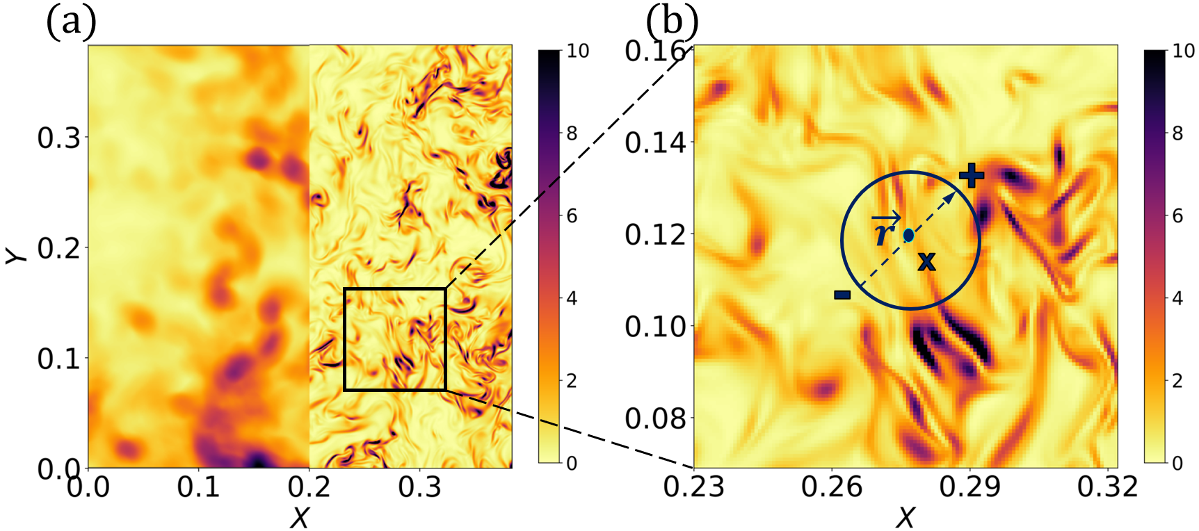
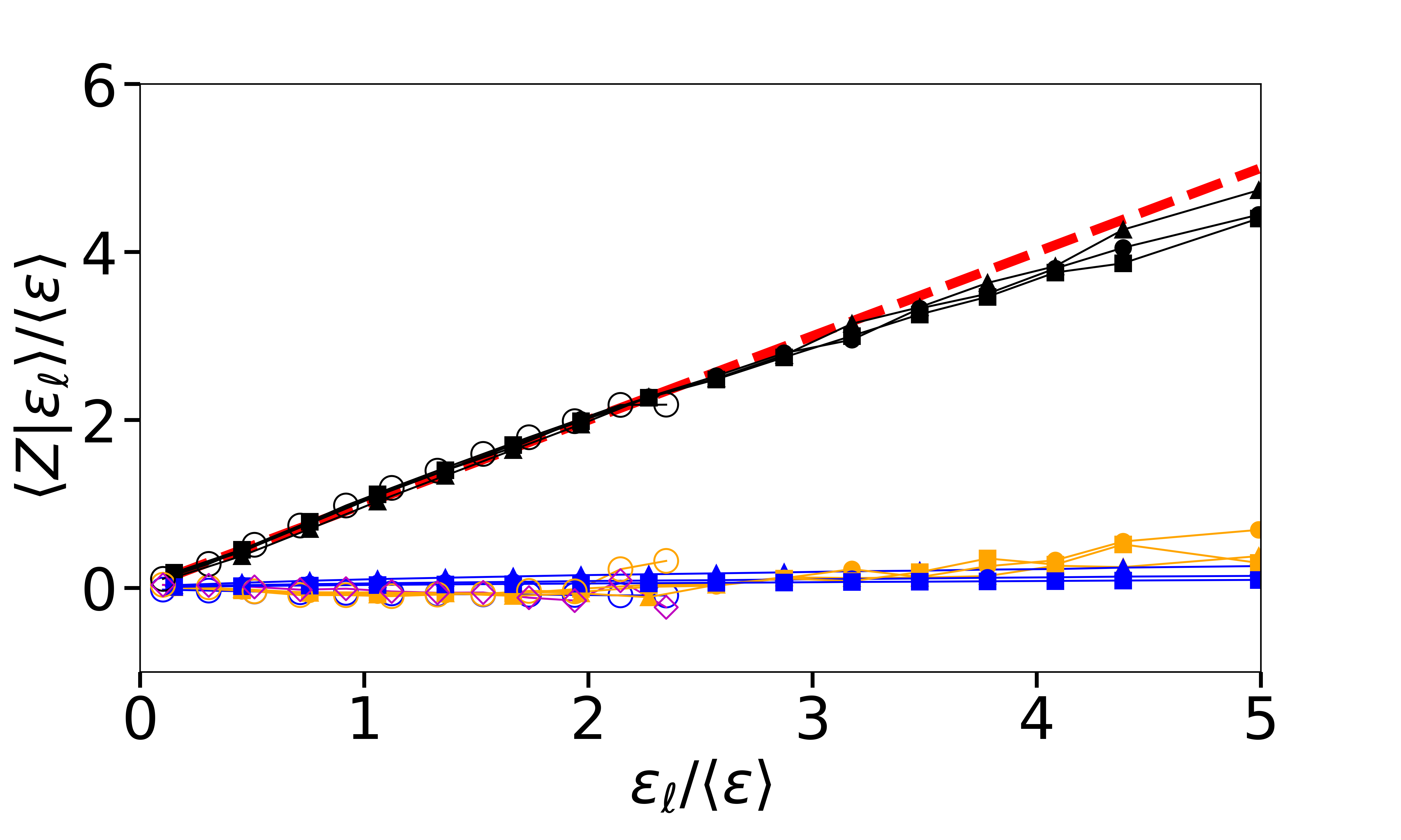
Figure 2 shows the conditional average $\langle\Phi_{\ell}|\epsilon_{\ell}\rangle$ as function of $\epsilon_{\ell}$. Statistics are computed using 2,000,000 randomly distributed spheres across the entire $8192^{3}$ isotropic turbulence dataset (isotropic8192) [31]. The analysis considers two length scales in the inertial range and one approaching the viscous range, namely $\ell=0.024L=60\eta$, $\ell=0.018L=45\eta$, and $\ell=0.012L=30\eta$, respectively, where $L=1.24$ is the integral scale and the Kolmogorov scale is $\eta=(\nu^{3}/\langle\epsilon\rangle)^{1/4}=4.98\times 10^{-4}$. It is apparent that the dominant terms are $\langle\Phi_{\ell}|\epsilon_{\ell}\rangle$ (black dots) and $\epsilon_{\ell}$ itself (red dash line with unit slope). These are equal for most of the range of $\epsilon_{\ell}$ for which reliable statistics can be collected. The good collapse $\langle\Phi_{\ell}|\epsilon_{\ell}\rangle\approx\epsilon_{\ell}$ provides clear support for the KRSH in the context of terms appearing in Eq. 2. Also plotted in Fig. 2 are the conditional averages of the pressure term, $\langle P_{\ell}|\epsilon_{\ell}\rangle$, and the viscous term, $\langle D_{\ell}|\epsilon_{\ell}\rangle$. We can see that the contribution of the pressure term (yellow squares) is negligible at all three length scales over most of the range. The viscous term (solid blue lines) is also negligibly small as expected. Approaching the largest values of $\epsilon_{\ell}/\langle\epsilon\rangle$ we observe saturation of $\Phi_{\ell}$ that is compensated by small rise of the pressure term (same results are obtained when using the full viscous dissipation $\nu(\partial u_{i}\partial x_{j})(\partial u_{i}\partial x_{j}+\partial u_{i}\partial x_{j})$ instead of the pseudo-dissipation $\nu(\partial u_{i}\partial x_{j})^{2}$).

Moreover, based on Eq. 4, we can conclude that $\langle\widetilde{d}k_{\ell}/dt|\epsilon_{\ell}\rangle\approx 0$, given that $\langle P_{\ell}|\epsilon_{\ell}\rangle\approx 0$, $\langle D_{\ell}|\epsilon_{\ell}\rangle\approx 0$, and $\langle\Phi_{\ell}|\epsilon_{\ell}\rangle\approx\epsilon_{\ell}$. To verify this result via explicit measurement, we computed the terms in Eq. 4 using the isotropic1024 [30] dataset. It has a smaller size of $1024^{3}$ grid points and a lower Reynolds number $R_{\lambda}=430$, but includes temporally consecutive snapshots allowing us to calculate time derivatives. Fig.  2 (open symbols) shows that $\langle\Phi_{\ell}|\epsilon_{\ell}\rangle\approx\epsilon_{\ell}$ still holds very well at this lower Reynolds number, that the pressure and viscous terms are again close to zero and that $\langle\widetilde{d}k_{\ell}/dt|\epsilon_{\ell}\rangle\approx 0$. We conclude that the data provide strong direct support to the KRSH relating $\Phi_{\ell}$ and $\epsilon_{\ell}$ and that the pressure and unsteadiness terms vanish in the inertial range.

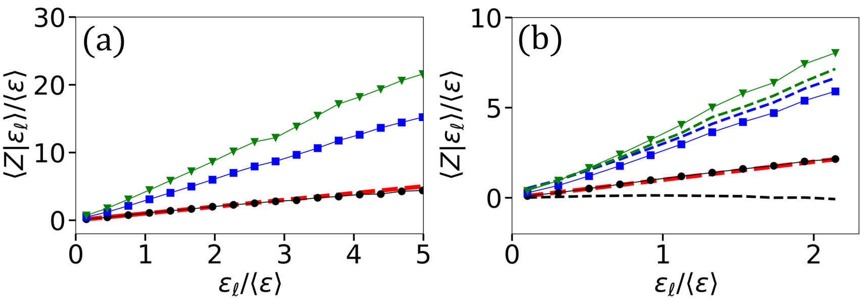
A further implication of KRSH relates to higher order moments. It implies that $\langle\Phi_{\ell}^{q}|\epsilon_{\ell}\rangle=\langle V_{\Phi}^{q}\rangle\,\epsilon_{\ell}^{q}$. In the inertial range, since $\Phi_{\ell}=\epsilon_{\ell}+W_{\ell}$ locally and instantaneously, raising to the $q$-power, expanding, and taking the conditional average yields $\langle\Phi_{\ell}^{q}|\epsilon_{\ell}\rangle=\sum_{n=0}^{q}\binom{q}{n}\,\,\epsilon_{\ell}^{q-n}\,\,\langle W_{\ell}^{n}|\epsilon_{\ell}\rangle.$ Thus, for KRSH to hold (i.e. for $\langle\Phi_{\ell}^{q}|\epsilon_{\ell}\rangle\propto\epsilon_{\ell}^{q}$) the conditional moments of $W_{\ell}$ must follow the same behavior, i.e., $\langle W_{\ell}^{n}|\epsilon_{\ell}\rangle\propto\epsilon_{\ell}^{n}$. Both the KRSH prediction for $\langle\Phi_{\ell}^{q}|\epsilon_{\ell}\rangle$ and $\langle W_{\ell}^{n}|\epsilon_{\ell}\rangle$ can be tested by measuring and plotting $\langle\Phi_{\ell}^{q}|\epsilon_{\ell}\rangle^{1/q}$ and $\langle W_{\ell}^{n}|\epsilon_{\ell}\rangle^{1/n}$ as function of $\epsilon_{\ell}$ and testing for linear behavior. Results are shown in Fig. 3 for $q=2,3$ and $n=2,3$. Clearly, the proportionality holds, with linear trends visible for these moment orders over the range of dissipation values.

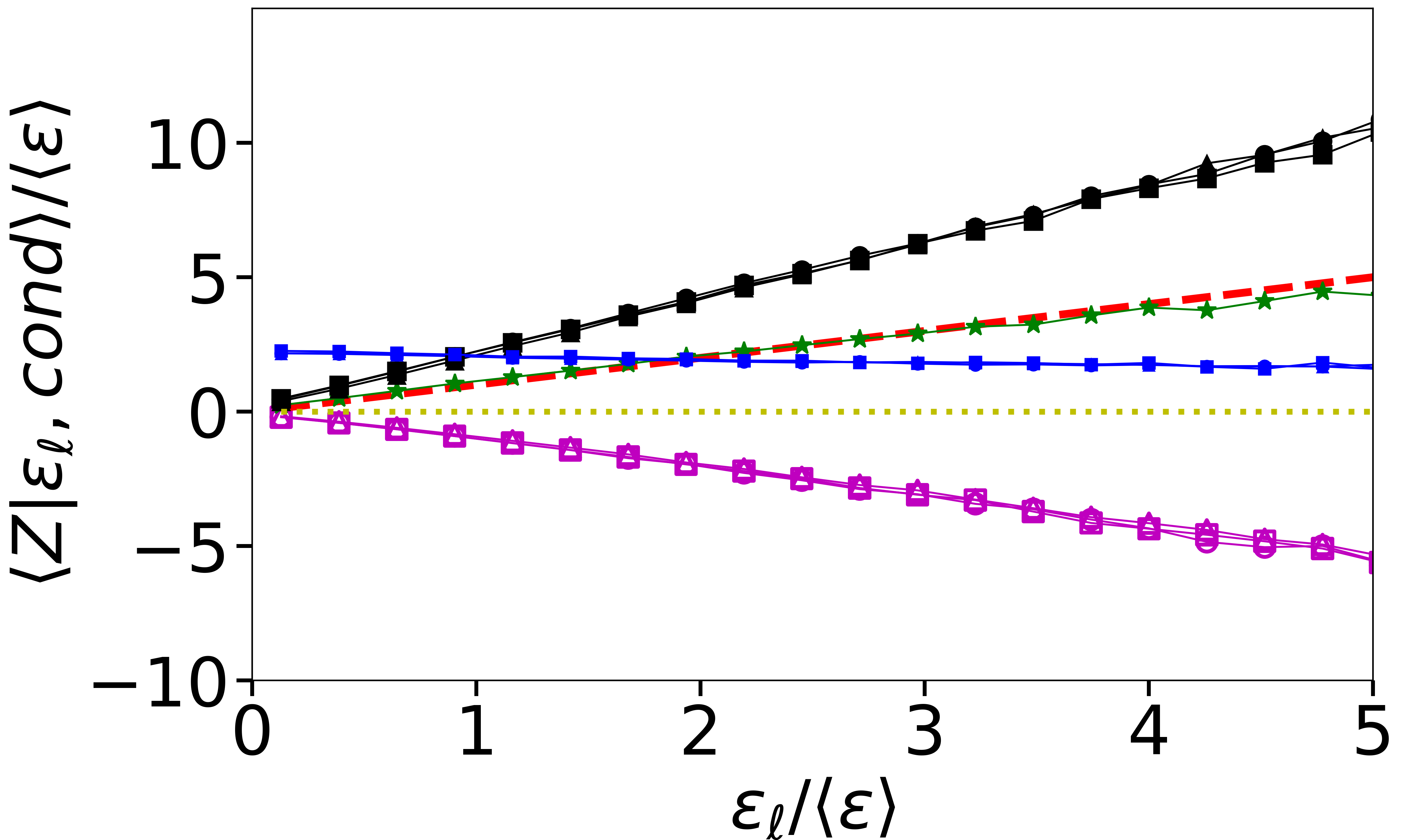
We now turn to further consequences of the KRSH that are directly related to the direction of the energy cascade, i.e. we examine if KRSH may be applicable even to those regions of the flow where $\Phi_{\ell}<0$, i.e., those displaying only inverse cascading, or $\Phi_{\ell}>0$, i.e, those displaying only forward cascading. An implication of KRSH is that the conditional average of only positive and only negative values of $\Phi_{\ell}$ should also be proportional to $\epsilon_{\ell}$. To investigate this prediction, we split the samples of $\Phi_{\ell}$ by its sign and perform conditional averaging based on $\epsilon_{\ell}$. We first observe that there are about twice as many samples with $\Phi_{\ell}>0$ than with $\Phi_{\ell}<0$, specifically, if ${\rm Pr}(\Phi_{\ell}>0|\epsilon_{\ell})$ and ${\rm Pr}(\Phi_{\ell}<0|\epsilon_{\ell})$ are the conditional total probabilities associated with signs of $\Phi_{\ell}$ in any $\epsilon_{\ell}$ bin, we measure ${\rm Pr}(\Phi_{\ell}>0|\epsilon_{\ell})/{\rm Pr}(\Phi_{\ell}<0|\epsilon_{\ell})\approx 2.0$ (see blue line in Fig. 4). In the inertial range, the ratio is approximately 2.0 (consistent with results from Ref. [32], who defined energy cascade rate by detailed evaluations of intersection of eddies and lifetimes). From normalization we conclude that ${\rm Pr}(\Phi_{\ell}>0|\epsilon_{\ell})\approx 2/3$ and ${\rm Pr}(\Phi_{\ell}<0|\epsilon_{\ell})\approx 1/3$. And since $\langle\Phi_{\ell}|\epsilon_{\ell}\rangle=\langle\Phi_{\ell}|\epsilon_{\ell},\Phi_{\ell}>0\rangle{\rm Pr}(\Phi_{\ell}>0|\epsilon_{\ell})+\langle\Phi_{\ell}|\epsilon_{\ell},\Phi_{\ell}<0\rangle{\rm Pr}(\Phi_{\ell}<0|\epsilon_{\ell})$ and the data already showed $\langle\Phi_{\ell}|\epsilon_{\ell}\rangle\approx\epsilon_{\ell}$, the KRSH further implies that $\langle\Phi_{\ell}|\epsilon_{\ell},\Phi_{\ell}<0\rangle\approx 3\,\epsilon_{\ell}-2\,\langle\Phi_{\ell}|\epsilon_{\ell},\Phi_{\ell}>0\rangle$. These predictions from RKSH are tested in Fig. 4, showing that $\langle\Phi_{\ell}|\epsilon_{\ell},\Phi_{\ell}>0\rangle\approx 2\,\epsilon_{\ell}$ and $\langle\Phi_{\ell}|\epsilon_{\ell},\Phi_{\ell}<0\rangle\approx-1\,\epsilon_{\ell}$. Clearly KRSH holds even for the positive and negative regions separately. For completeness, we also show the conditional average of the traditional third-order longitudinal structure function, which under the assumption of isotropy and KRSH follows $-(5/4\ell)\langle(\delta u_{j}\hat{n}_{j})^{3}|\epsilon_{\ell}\rangle=\epsilon_{\ell}$.

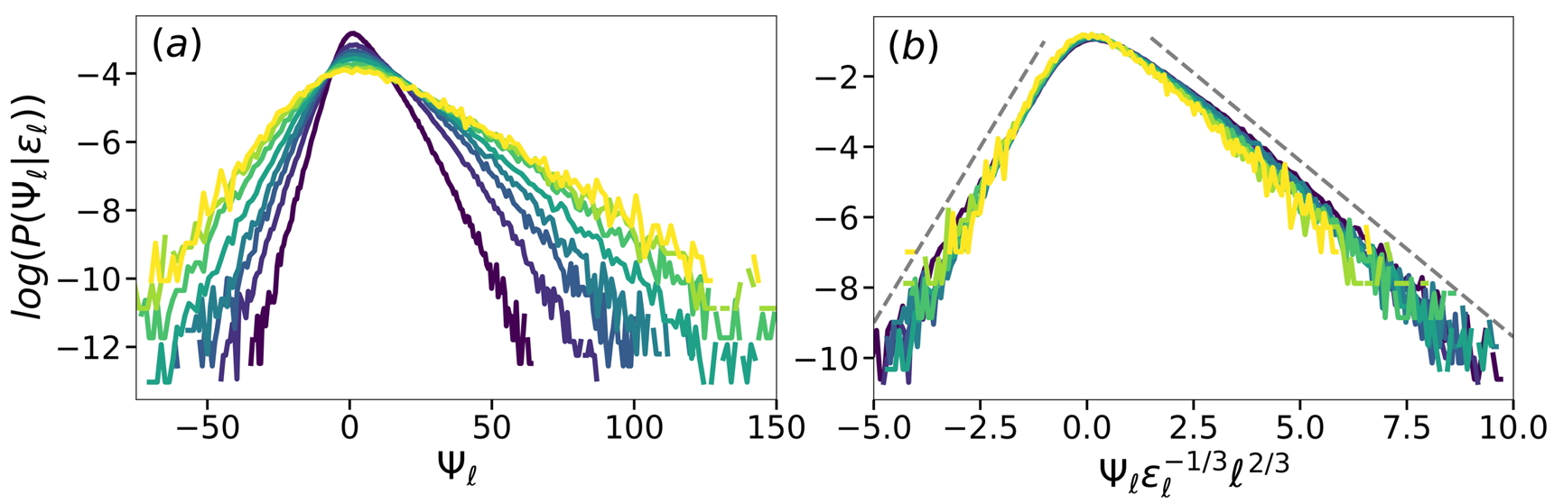
Next, following Ref. [20] we examine the fluctuation relation from non-equilibrium thermodynamics, but instead of using the overall dissipation rate to define the characteristic eddy turn-over timescale, we here use conditioning on various values of local dissipation $\epsilon_{\ell}$. Figure 5(a) shows the conditional PDF $P(\Psi_{\ell}|\epsilon_{\ell})$ of the entropy generation rate $\Psi_{\ell}=\Phi_{\ell}/k_{\ell}$ for $\ell/\eta=45$, conditioned for various values of $\epsilon_{\ell}$ ranging from $\epsilon_{\ell}/\langle\epsilon\rangle=0.15$ to 4.2. As in [20], exponential tails are found, with steeper slopes on the negative side than on the positive one, and approximately twice as steep. Remarkably, when multiplying $\Psi_{\ell}$ by the corresponding local turn-over time-scale $\tau_{\ell}=\epsilon_{\ell}^{-1/3}\ell^{2/3}$ where $\epsilon_{\ell}$ is the value used to bin the data, excellent collapse is observed, see Fig. 5 (b). If the PDFs are approximated as pure exponentials, with slope magnitudes $\alpha_{-}$ for $\Psi_{\ell}<0$ and $\alpha_{+}$ for $\Psi_{\ell}>0$, it is evident from Fig. 5(b) that $\alpha_{+}\approx 1$ and $\alpha_{-}\approx 2$. For such two-sided exponential PDFs, it is easy to show that ${\rm Pr}(\Psi_{\ell}<0)/{\rm Pr}(\Psi_{\ell}>0)=\alpha_{+}/\alpha_{-}$, consistent with the 1:2 ratio discussed above, independent of $\epsilon_{\ell}$.

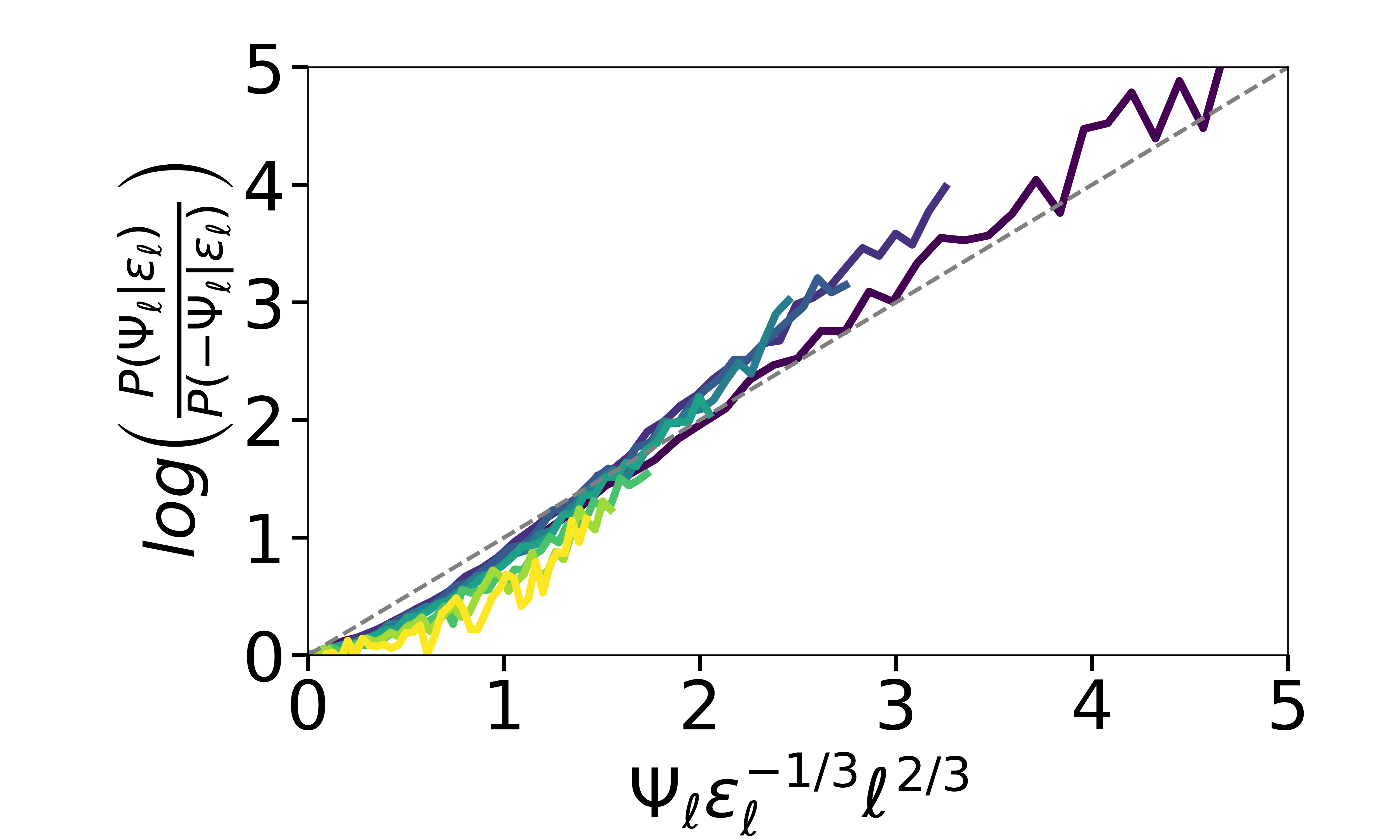
Finally, the FR can be tested by plotting $\log[P(\Psi_{\ell}|\epsilon_{\ell})/P(-\Psi_{\ell}|\epsilon_{\ell})]$ versus $\Psi_{\ell}\tau_{\ell}$ (see Fig. 6). The result shows good collapse and an approximately linear trend (especially at $\Psi_{\ell}\tau_{\ell}>1$, thus providing empirical/approximate support for the fluctuation relation for turbulence even when conditioning on different values of $\epsilon_{\ell}$, and using $\epsilon_{\ell}$ to establish the relevant turn-over time-scale. For the exponential approximation of the conditional PDFs, the slope in the FR plot is simply $\alpha_{-}-\alpha_{+}$, which is nearly unity (as observed originally in [20]), and quite consistent with $\alpha_{-}\approx 2$ while $\alpha_{+}\approx 1$.

In summary, we examined the KRSH involving the local dissipation $\epsilon_{\ell}$ in the context of an equation (Eq. 2) derived exactly from the Navier-Stokes equations. Results from two DNS of forced isotropic turbulence provided strong support for the validity of KRSH for the cascade rate $\Phi_{\ell}$, its moments, and also for moments of other terms appearing in the dynamical equation. Furthermore the data support a strong version of the KRSH when positive and negative cascade rates are considered separately, each of which scale proportional to $\epsilon_{\ell}$. Finally, the fluctuation relation from non-equilibrium thermodynamics is shown to hold to a good approximation, relating the probability of forward and backward cascade events using the local time-scale based on $\epsilon_{\ell}$ and $\ell$. This result represents the first time that the fluctuation relation is observed in the inertial range of 3D turbulence (not model systems), based on conditional averages as in the KRSH.

Present findings connecting KRSH directly to a dynamical equation derived from the Navier-Stokes equations as well as to basic principles of non-equilibrium thermodynamics could help in developing improved theories and models of the turbulence cascade process. Additional questions arise, such as what are the effects of time-averaging in defining the entropy generation rate $\Psi_{\ell}$ (we have applied the FR at some turn-over time $t=\tau_{\ell}$ and tested FR only as far as the fluctuations in $\Psi_{\ell}$ are concerned), what occurs when $\ell$ approaches limits of the inertial range, and do the results hold for flows with mean shear and walls? Finally, it bears recalling that the FR is applicable to systems in which the microscopic dynamics are time-reversible (but, see discussion in [33]). As argued in [20], we here regard the microscopic degrees of freedom to be the inertial-range eddies smaller than $\ell$ whose evolution is governed by nearly inviscid, thus time-reversible, dynamics at least for some small finite time. While the actual turbulent state we are analyzing is already far from equilibrium so that the overall statistics of velocity increments (and $\Phi_{\ell}$, $\Psi_{\ell}$) display the established asymmetry, the actual dynamics in the inertial range can be time-reversed for some time [23]. Still, significant questions remain about connections between non-equilibrium thermodynamics and 3D turbulence in the inertial range.

Acknowledgements: We thank R. Hill for comments on an early draft of this work. The work is supported by NSF (CSSI-2103874) and the contributions from the JHTDB team are gratefully acknowledged.

References

- Richardson [1922] L. F. Richardson, Weather Prediction by Numerical Process (Cambridge university press, 1922).
- Kolmogorov [1941] A. N. Kolmogorov, C.R. Acad. Sci. URSS 30, 301 (1941).
- Frisch [1995] U. Frisch, Turbulence: the legacy of AN Kolmogorov (Cambridge University Press, 1995).
- Kolmogorov [1962] A. N. Kolmogorov, J. of Fluid Mechanics 13, 82 (1962).
- Meneveau and Sreenivasan [1991] C. Meneveau and K. R. Sreenivasan, Journal of Fluid Mechanics 224, 429 (1991).
- Stolovitzky et al. [1992] G. Stolovitzky, P. Kailasnath, and K. R. Sreenivasan, Physical Review Letters 69, 1178 (1992).
- Praskovsky [1992] A. A. Praskovsky, Physics of Fluids A: Fluid Dynamics 4, 2589 (1992).
- Wang et al. [1996] L.-P. Wang, S. Chen, J. G. Brasseur, and J. C. Wyngaard, Journal of Fluid Mechanics 309, 113 (1996).
- Iyer et al. [2015] K. P. Iyer, K. R. Sreenivasan, and P. K. Yeung, Physical Review E 92, 063024 (2015).
- Yeung and Ravikumar [2020] P. K. Yeung and K. Ravikumar, Physical Review Fluids 5, 110517 (2020).
- Lawson et al. [2019] J. M. Lawson, E. Bodenschatz, A. N. Knutsen, J. R. Dawson, and N. A. Worth, Physical Review Fluids 4, 022601 (2019).
- Hill [2002] R. J. Hill, Journal of Fluid Mechanics 468, 317 (2002).
- Yasuda and Vassilicos [2018] T. Yasuda and J. C. Vassilicos, Journal of Fluid Mechanics 853, 235 (2018).
- Monin and Yaglom [1975] A. S. Monin and A. M. Yaglom, Statistical Fluid Mechanics: Mechanics of Turbulence (MIT Press, 1975).
- Danaila et al. [2001] L. Danaila, F. Anselmet, T. Zhou, and R. A. Antonia, Journal of Fluid Mechanics 430, 87–109 (2001).
- Duchon and Robert [2000] J. Duchon and R. Robert, Nonlinearity 13, 249 (2000).
- Eyink [2002] G. L. Eyink, Nonlinearity 16, 137 (2002).
- Dubrulle [2019] B. Dubrulle, Journal of Fluid Mechanics 867, P1 (2019).
- Yao et al. [2023a] H. Yao, M. Schnaubelt, A. Szalay, T. Zaki, and C. Meneveau, Journal Fluid Mechanis (accepted) (2023a).
- Yao et al. [2023b] H. Yao, T. A. Zaki, and C. Meneveau, Journal of Fluid Mechanics 973, R6 (2023b).
- Chorin [1991] A. J. Chorin, Communications in Mathematical Physics 141, 619 (1991).
- Paladin and Vulpiani [1987] G. Paladin and A. Vulpiani, Physics Reports 156, 147 (1987).
- Vela-Martín and Jiménez [2021] A. Vela-Martín and J. Jiménez, Journal of Fluid Mechanics 915, A36 (2021).
- Castaing [1996] B. Castaing, Journal de Physique II 6, 105 (1996).
- Evans et al. [1993] D. J. Evans, E. G. D. Cohen, and G. P. Morriss, Physical Review Letters 71, 2401 (1993).
- Gallavotti and Cohen [1995] G. Gallavotti and E. G. D. Cohen, Physical Review Letters 74, 2694 (1995).
- Fuchs et al. [2020] A. Fuchs, S. M. D. Queirós, P. G. Lind, A. Girard, F. Bouchet, M. Wächter, and J. Peinke, Physical Review Fluids 5, 034602 (2020).
- Zonta and Chibbaro [2016] F. Zonta and S. Chibbaro, Europhysics Letters 114, 50011 (2016).
- Porporato et al. [2020] A. Porporato, M. Hooshyar, A. D. Bragg, and G. Katul, Proc. of the Royal Society A 476, 20200468 (2020).
- Li et al. [2008] Y. Li, E. Perlman, M. Wan, Y. Yang, C. Meneveau, R. Burns, S. Chen, A. Szalay, and G. Eyink, Journal of Turbulence , N31 (2008).
- Yeung et al. [2015] P. K. Yeung, X. Zhai, and K. R. Sreenivasan, Proceedings of the National Academy of Sciences 112, 12633 (2015).
- Cardesa et al. [2017] J. I. Cardesa, A. Vela-Martín, and J. Jiménez, Science 357, 782 (2017).
- Gallavotti [2020] G. Gallavotti, The European Physical Journal E 43, 1 (2020).