Formation Tracking for a Multi-Auv System Based on an Adaptive Sliding Mode Method in the Water Flow Environment

As shown in Fig. 3, the state vector (position and posture) of the AUV is defined as $\bm{\eta}=\left[\bm{\eta}_{1}^{\mathrm{T}}\ \bm{\eta}_{2}^{\mathrm{T}}\right]^{\mathrm{T}}\in\mathbb{R}^{6}$, where $\bm{\eta}_{1}=\left[x\ {y}\ {z}\right]^{\mathrm{T}}\in\mathbb{R}^{3}$ is the vector of vehicle position coordinates in an earth-fixed or inertial referenced frame and $\bm{\eta}_{2}=\left[\phi\ {\theta}\ {\psi}\right]^{\mathrm{T}}\in\mathbb{R}^{3}$ is the vector of vehicle’s Euler-angle coordinates in an inertial reference frame. At the same time, the dynamic vector of the AUV is defined as $\bm{v}=\left[\bm{v}_{1}^{\mathrm{T}}\ \bm{v}_{2}^{\mathrm{T}}\right]^{\mathrm{T}}\in\mathbb{R}^{6}$, where $\bm{v}_{1}=\left[u\ v\ w\right]^{\mathrm{T}}\in\mathbb{R}^{3}$ is the vector of vehicle linear velocity expressed in the vehicle-fixed reference frame, and $\bm{v}_{2}=\left[p\ q\ r\right]^{\mathrm{T}}\in\mathbb{R}^{3}$ is the vector of vehicle angular velocity expressed in the body-fixed frame.

The parameters of the AUV’s 6-DOF model is show in Table 1. The vehicle-fixed linear and angular velocities and the time derivative of the earth-fixed vehicle coordinates are related by the following equations:

where $\bm{R}_{I}^{C}$ is the rotation matrix expressing the linear velocity transformation from the inertial earth-fixed frame to the body-fixed frame, and the angular velocity transformation matrix $\bm{T}\in\mathbb{R}^{6}$ is Jacobian matrix, which can be both found in former literatures [35, 36, 37].

Considering the coordinate systems illustrated in Fig. 3, the dynamic equations of the AUVs in the vehicle-fixed reference frame are written as

where $\bm{q}=\left[u\ v\ w\ p\ q\ r\ \right]^{\mathrm{T}}$ is the ROV spatial velocity state vector with respect to its body-fixed reference frame, and $\bm{e}=\left[x\ y\ z\ \phi\ \theta\ \psi\right]^{\mathrm{T}}$ is the position and orientation state vector with respect to the inertial reference frame. The spatial transformation matrix between the inertial frame and the AUV’s body-fixed frame can be defined through the Euler angle transformation, denoted by $\mathbf{J}(\bm{e})\in\mathbb{R}^{6\times 6}$. The term $\mathbf{M}(\bm{q})\in\mathbb{R}^{6\times 6}$ is the inertia matrix including the added mass effects. $\mathbf{C}(\bm{q})\in\mathbb{R}^{6\times 6}$ is the matrix of centrifugal and Coriolis terms. $\mathbf{D}(\bm{q})\in\mathbb{R}^{6\times 6}$ is the drag matrix, with that $\mathbf{g}(\bm{e})\in\mathbb{R}^{6\times 6}$ is the vector of gravity and buoyancy forces and moments. $\bm{\tau}\in\mathbb{R}^{6\times 1}$ is the matrix of control forces and moments acting on the AUV center of mass [25, 38, 39]. $\bm{\tau}_{c}\in\mathbb{R}^{6\times 1}$ is the matrix of forces and torques produced by the water flow which is acting on the AUV working under the water. Note that as the disturbance is caused by the water flow, $\bm{\tau}_{c}$ is complex and changeable, so that it is difficult to build a model.

The dynamic equation of motion of AUVs in the inertial reference frame can be presented as

where $\mathbf{M}_{e}(\bm{e})=\mathbf{J}^{-\mathrm{T}}\mathbf{M}\mathbf{J}^{-1}$, $\mathbf{C}_{e}(\bm{q},\bm{e})=\mathbf{J}^{-\mathrm{T}}\left[\mathbf{C}-\mathbf{M}\mathbf{J}^{-1}\dot{\mathbf{J}}\right]\mathbf{J}^{-1}$, $\mathbf{D}_{e}(\bm{q},\bm{e})=\mathbf{J}^{-\mathrm{T}}\mathbf{D}\mathbf{J}^{-1}$, and $\mathbf{g}_{e}(e)=\mathbf{J}^{-\mathrm{T}}\mathbf{g}$. The system dynamics are not exactly known, because the AUV dynamics are underactuated and dominated by hydrodynamic loads. It is difficult to accurately measure or estimate the hydrodynamic coefficients that are valid for AUVs’ operating conditions. Therefore, the system dynamics can be written as the sum of estimated dynamics $\hat{\bm{f}}$ and the unknown dynamics $\tilde{\bm{f}}$ and we have

The estimated dynamics vector is defined as

with $\hat{\bm{h}}(\bm{q},\bm{e})=\hat{\mathbf{C}}_{e}(\bm{q},\bm{e})\bm{e}+\hat{\mathbf{D}}_{e}(\bm{q},\bm{e})\bm{e}+\hat{\mathbf{g}}_{e}(\bm{e})$ and the unknown dynamics vector are defined as

with $\tilde{\bm{h}}(\bm{q},\bm{e})=\tilde{\mathbf{C}}_{e}(\bm{q},\bm{e})\bm{e}+\tilde{\mathbf{D}}_{e}(\bm{q},\bm{e})\bm{e}+\tilde{\mathbf{g}}_{e}(\bm{e})$. $\tilde{\mathbf{M}}_{e}$, $\tilde{\mathbf{C}}_{e}$, $\tilde{\mathbf{D}}_{e}$, $\tilde{\mathbf{g}}_{e}$ represents the unknown items. In (6), as the additional disturbance is bounded in the environment, the nonlinear uncertainty vector $\tilde{\bm{f}}$ and its time domain differential could be assumed to be bounded.

In the previous researches on multi-AUV systems, there are relatively few researches on the ocean current. However, in practice, the influence of the current cannot be ignored, and it is even a very important factor for the successful tasks of the AUV formation. The existence of the water flow can generate drifting motions, making AUVs deviate from the predetermined trajectories.

In the inertial coordinate system, the influence of the regular current can be expressed as the vector $\bm{\tau}_{e,f}$ of the force and torque. $\tilde{\bm{\tau}}_{e,f}$ is the force and torque vector generated by the propeller to offset the disturbance of ocean current, then we have $\tilde{\bm{\tau}}_{e,f}=-\bm{\tau}_{e,f}$ in the ideal condition. It is either a constant or as a quantity that transforms slowly and regularly. For the wind currents and other flows, the speeds change as time varying, generally after the wind stops the flow can continue change for a period. Such currents’ information are hard to predict or measure. In the inertial coordinate system, it is assumed that the change of current disturbance is $\bm{d}_{o}\in\mathbb{R}^{6\times 1}$ equivalent to $\bm{d}_{e,o}$ in the body-fixed frame. If $\bm{d}_{e,o}$ is bounded, adaptive higher-order controller adopted in this paper can deal with the disturbances in a certain range and ensure the normal operation of AUVs in formation. Considering the influence of regular current and variable flow, the total influence on the AUVs is

where $\bm{\tau}_{e,c}=\mathbf{J}^{-\mathrm{T}}\bm{\tau}_{c}$ as depicted in (3).

Since the pattern of ocean current is time-varying, it is difficult to find a unified mathematical model, and the general disturbance of ocean current is bounded. Therefore, we build a function to verify the effectiveness of the algorithm by means of a trial water flow example [40].

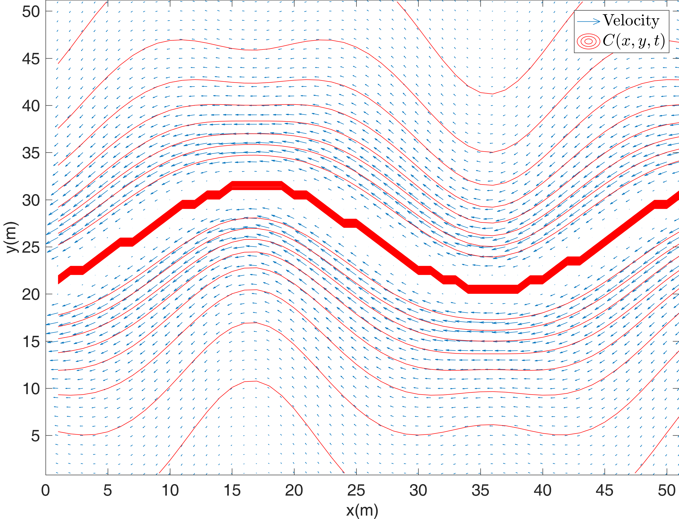
The 3-D working environment of AUVs is represented by cartesian coordinate system. Let $z=0$ be the water surface level, and the $z$-axis points to the bottom of the sea or river. The working space is stratified by depth $z$ into $N$ ($N\in\mathbb{N}^{+}$) layers, and each layer is an $x$-$O$-$y$ plane of two dimensions (2-D). Each $z=N$ ($N=1,2,3,...$) plane is rasterized, and each grid is a square with equal side length of $1$ ($m$). The currents in the areas within each grid can be regarded as the same. An east-west flow field with a meandering north-south flow field is adopted, and the mathematical expression of the flow function $C(x,y,t)$ at time $t$ is

In (8), $B(t)=\left(B_{0}+E\cos(\omega t+\theta)\right)$, $B_{0}=1.2$, $w=0.4$, $\theta=\pi/2$, $c=0.12$, $k=0.82$, $E=0.3$. According to the flow function, the current velocity can be calculated as

where $U(x,y,t)$ and $V(x,y,t)$ are the velocity components of the water flow in the $x$ and the $y$ directions at time $t$, respectively.

Suppose that the water flow field in the workspace of a depth of $z\in[-20\ 0]$ ($m$) is equally divided into three layers, and the velocity gradually decreases from the water surface to the bottom layer. $\left|V_{ci}\right|$ ($i=1,2,3$) denotes the the module value of the current velocity in each layer, with $\left|V_{c1}\right|=2.4\left|V_{c2}\right|=4\left|V_{c3}\right|$. Then the 2-D current field is illustrated in Fig. 4 and the 3-D current field is illustrated in Fig. 4. As shown in Fig. 4, the arrow indicates the direction of the current at this position, and the length of the arrow is proportional to the velocity of the current. Taking this kind of water flow field as an example, simulations to test the proposed algorithm can be implemented.

The sliding order $r$ refers to the number of zeros of the continuous full derivatives which equal to zero on the sliding mode surface of the sliding mode variable $s$. The sliding set of order $r$ related to the sliding mode surface is defined as the equation $s=\dot{s}=\ddot{s}=\ldots=s^{(r-1)}=0$. If the sliding set of order $r$ exists, and it is assumed to be the local set in the sense of Filippov, the motion satisfying this equation is named $r$ order sliding mode about the sliding mode surface $s(x,t)=0$, and the order $r-1$ is called the relative order of the system.

The sliding order of the AUV system is designed as a number of continuous total derivatives of in the vicinity of the sliding mode. It fixes the dynamics smoothness degree. The $r$-th order sliding mode is determined by the equation:

The main problem of higher-order sliding mode control is the increment of the demanded information. For example, the system degree is 3, and then a 3-sliding controller needs an input control parameters $\sigma=\dot{\sigma}=\ddot{\sigma}=\sigma^{(r-1)}$. Fortunately, the super twisting algorithm that we adopt needs only the measurement of $\sigma$. Then the higher-order controller’s action $u_{\textrm{HOSMC}}$ can be defined as

Note that $u_{1}$ and $u_{2}$ are both functions of time $t$, corresponding respectively to a continuous function of the sliding mode surface and an integration of the sliding mode surface in the time domain [41]:

and

where $u_{max}\in N^{+}$, and can be normalize to 1. The remaining parameters are set in the simulations. According to [42], the sufficient conditions to ensure convergence to the origin for the sliding mode plane in finite time is

where $W$, $\rho$, $\lambda$, $\Phi$ are positive constants to be adjusted in the simulation.

The algorithm does not need any differential information of sliding mode surface $\sigma$ in time domain, so the computation burden of controller is greatly reduced. Although the algorithm has good robustness, when $\sigma$ is very small, the control signal output is not Lipshitz, which may cause some noise in control output. In the simulations, parameters of the controller are continuously adjusted to find the most suitable values.

On the phase plane defined by the estimable second-order state equation (5), a first order dynamic equation is designed to represent the switching surface $\sigma$:

where $\bm{M}\in\mathbb{R}^{6}$ is positive definite diagonal matrix for the expected error response. When $\sigma=0$, the dynamic response of the system is as expected, which means $\sigma$ can represent the difference between the current system state and the desired state. $\bm{\varepsilon}=\bm{e}-\bm{e}_{d}$ represents the tracking error between the actual system and the desired system. $\bm{e}_{d}$ is the desired AUV position and attitude vector. Substituting $\bm{\varepsilon}$ in (15), we have

where $\dot{\bm{e}}_{r}=\dot{\bm{e}}_{d}-2\mathbf{M}\bm{\varepsilon}-\mathbf{M}^{2}\int\bm{\varepsilon}dt$, and $\bm{r}_{r}$ represents the reference trajectory of the AUV.

As shown in (11), $u_{\textrm{HOSMC}}$ represents the control force acting on the AUV’s center of mass; $u_{1}$ and $u_{2}$ represent the equivalent control and switching control respectively. The equivalent control $u_{1}$ is a continuous function based on the AUV’s model. If there is no uncertainty in the system dynamics, the equivalent control rate can achieve the desired state. However, AUV has a dynamic model and works with external disturbances, so the controller should include a switching control quantity $W\operatorname{sign}(\sigma)$, where $W$ is the upper limit of system model parameter uncertainty. the switching control $u_{2}$ could be a discontinuous feedback function, which is mainly used to compensate the differential characteristics and external disturbances of the expected AUV’s dynamics, so as to make the system stable. However, the switching control rate function is easy to make the system oscillate near the switching surface, causing the chattering phenomenon, so it is necessary to redesign an adaptive switching controller to help the system to achieve stability.

According to the super twisting algorithm, the control law can be written as

Then the control equation is

Let $\hat{\bm{f}}_{r}=\hat{\mathbf{M}}_{e}(\bm{e})\ddot{\bm{e}}_{r}+\hat{\bm{h}}(\bm{q},\bm{e})$ be the predictable dynamic vector $\hat{\bm{f}}$’s equivalent control quantity, then the system input control quantity obtained based on the equivalent control law is

For the system dynamics model without external disturbance, the equivalent control law of $u_{1}$ could meet the requirements. Otherwise, the switching control $u_{2}$ needs to be added adaptive characteristic in order to achieve robustness.

By adding an adaptive control link to the higher-order sliding mode controller, we can obtain a chattering-free and anti-interference controller. The controller’s block diagram is shown in Fig. 5.

As mentioned above, the switching control $u_{2}$ becomes the adaptive controller after adding the adaptive characteristic to it. In order to replace the discontinuous function in the switching controller, we use a continuous adaptive control law

where $\mathbf{K}\in\mathbb{R}^{6\times 6}$ is a positive definite diagonal matrix relative to the convergence rate of the controller. $\tilde{\bm{f}}_{est}$ is an adaptive term realizing the estimation of lumped parameter uncertainty vector $\tilde{\bm{f}}$ in (6). The renewal rate of $\tilde{\bm{f}}$ is designed as

where $\bm{\Gamma}\in\mathbb{R}^{6\times 6}$ is the positive definite diagonal matrix related to the adaptive rate. The adaptive term $\tilde{\bm{f}}_{est}$ is the error estimation of sliding mode surface $\sigma$, which can make the predicted system dynamic state more close to the actual system dynamic state under unknown disturbances. If $\tilde{\bm{f}}_{est}$ is bounded, $\dot{\tilde{\bm{f}}}_{est}$ is also bounded.

If the speed of the formation is slow and $\tilde{\bm{f}}$ is relatively small, then $\bm{w}$ decreases with the effect of adaptive control law. Then the inequality in Assumption. 22 is easier to implement. Even in the worst case, condition in (22) can be meet by adjusting $\mathbf{K}$ and $\mathbf{\Gamma}$.

As we can model the AUV’s dynamics in the physical engine simulation system, a kind of model predictive control method is combined into the adaptive higer-order sliding mode controller to make the control output more smoother.

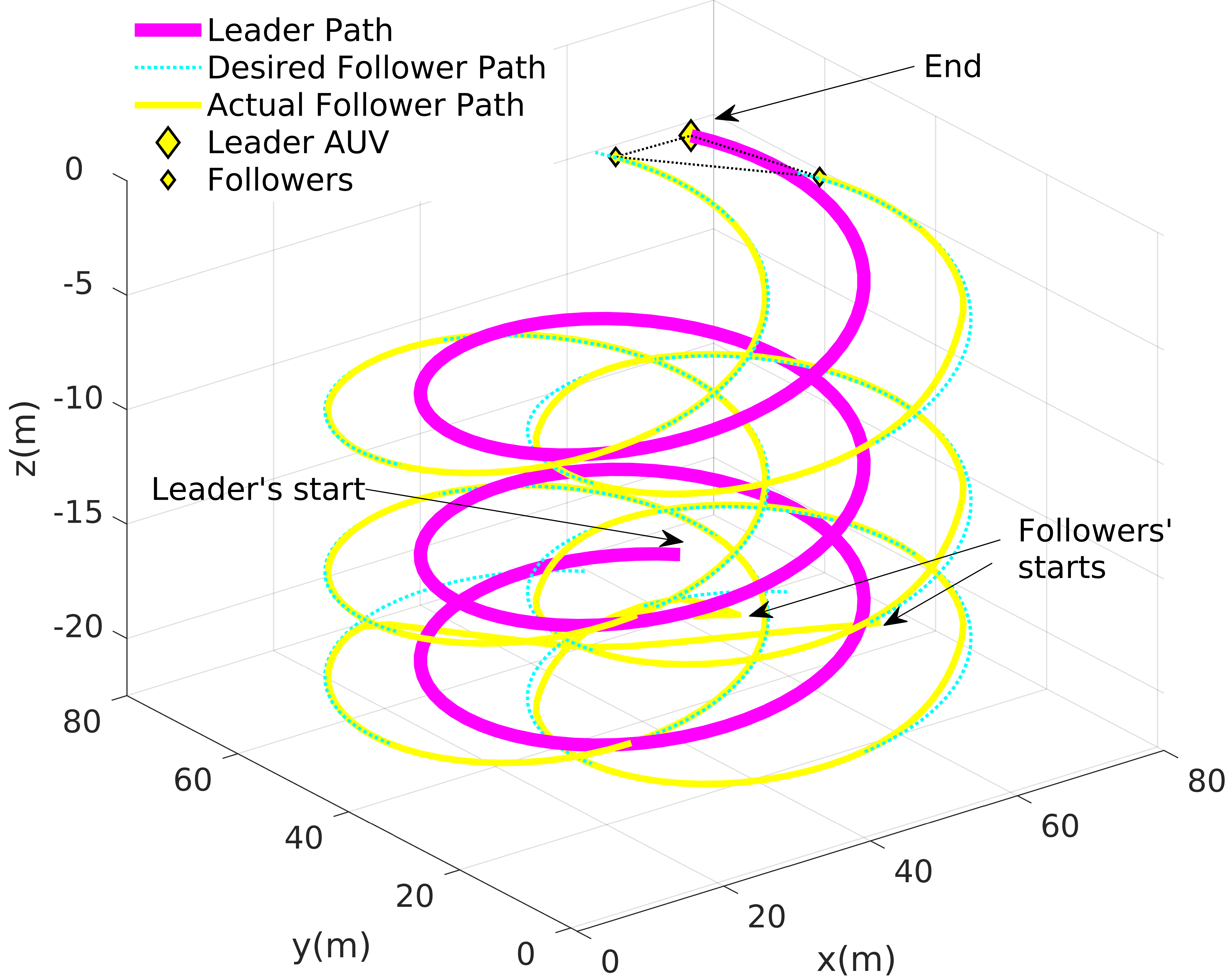
Considering a team of 3 AUVs in a triangular formation tracking an arbitrary curve path, we assume that the leader AUV moves first and all the followers have essential sensors to contact with the leader and acquire essential informations such as relative distances and angles to the leader. The control object is to make the followers track the desired paths simultaneously as accurate as possible. The whole formation is kept and the path is tracked in this way. The controller adjusts the velocities and the directions of the AUVs in the formation to achieve this goal. In the simulations, we set the time-varied water flow disturbance vector ${\bm{d}_{o}}=[{C_{x}}\ {C_{y}}\ {0}\ {0}\ {0}\ {C_{z}}]$ equivalent to the parameter $\bm{d}$ depicted in Fig. 5. In this way the water flow influence is resolved into three quantities in the $x,y,z$ directions respectively, which is convenient for simulation. As the current velocity is assumed to be bounded, let $\left(C_{x},C_{y},C_{z}\right)\in[-20\ 20]$ $(\mathrm{N})$.

Based on the formation control algorithm, 3 AUVs form a triangular formation at the starting position. The leader runs along the desired path and meanwhile generates the desired path of the 2 followers. The follower AUV also runs along the desired path according to the adaptive higher-order sliding mode control algorithm, until the formation reaches the target position. During the tracking procedure, the trajectory tracking and formation keeping are both well maintained. As shown in Fig. 8, the formation moves along the spiral trajectory in triangular shape. The formation tracking test achieves good results.

Taking the left follower as the research object, the control effects in three directions of $x$, $y$ and $z$ are analyzed, i.e. $\tau_{u}$, $\tau_{v}$ and $\tau_{w}$ correspondingly. $\tau_{u}$ comprises two parts of $u_{1}$ and $u_{2}$ as mentioned above. The input of the controller in $x$ direction is show in Fig. 9.

Similarly, the controller input in the $y$ direction is also comprised of $u_{1}$ and $u_{2}$ as shown in Figure. 10. In the $z$ direction, the controller input is shown in Figure. 11. From the simulation results, we could find that the contoller input $u_{1}$ are bounded and smooth, and $u_{2}$ are bound pulses which are realizable. Unlike the control inputs in the $x$ and $y$ directions, $u_{2}$ in $z$ direction tends to be zero. This is because the water flow is layered in the 3-D space. The forces of the flow is parallel with the $x-y$ plane without vertical influence in the $z$ axis.

Helical trajectory formation tracking results are smooth and interference resistible as illustrated in Fig. 8. In the formation trajectory tracking process, we use the position error value $e$ as the $x$ axis and the speed error value $de$ as the $y$ axis. Then the system phase trajectories with the proposed adaptive higher-order sliding mode controller are depicted in Fig. 12 in the $x$, $y$ and $z$ axis respectively.

As show in the figure, system phase trajectories converge to the expected location after certain times of iterations. In the $x$, $y$ and $z$ directions, the system trajectories chatter a little after each movement of the formation leader. That’s because the algorithm need some iterations to calculate the control input. After the calculation is finished, the trajectories converge.

For the position and velocity errors in the 3 directions of $x$, $y$ and $z$, the errors are limited to a small range after the sliding mode control algorithm converges. Table. 2 gives the tracking error analysis, using the root mean squared error (RMSE) to measure the velocity error and the position error from the time $t=0$. The maximum and minimum errors of the system after convergence are recorded. In this experiment, the convergence moment is $t=11$ ($s$). The velocity error and position error do not converge to zero, but fluctuate regularly within a limited range, which is acceptable in practical applications.

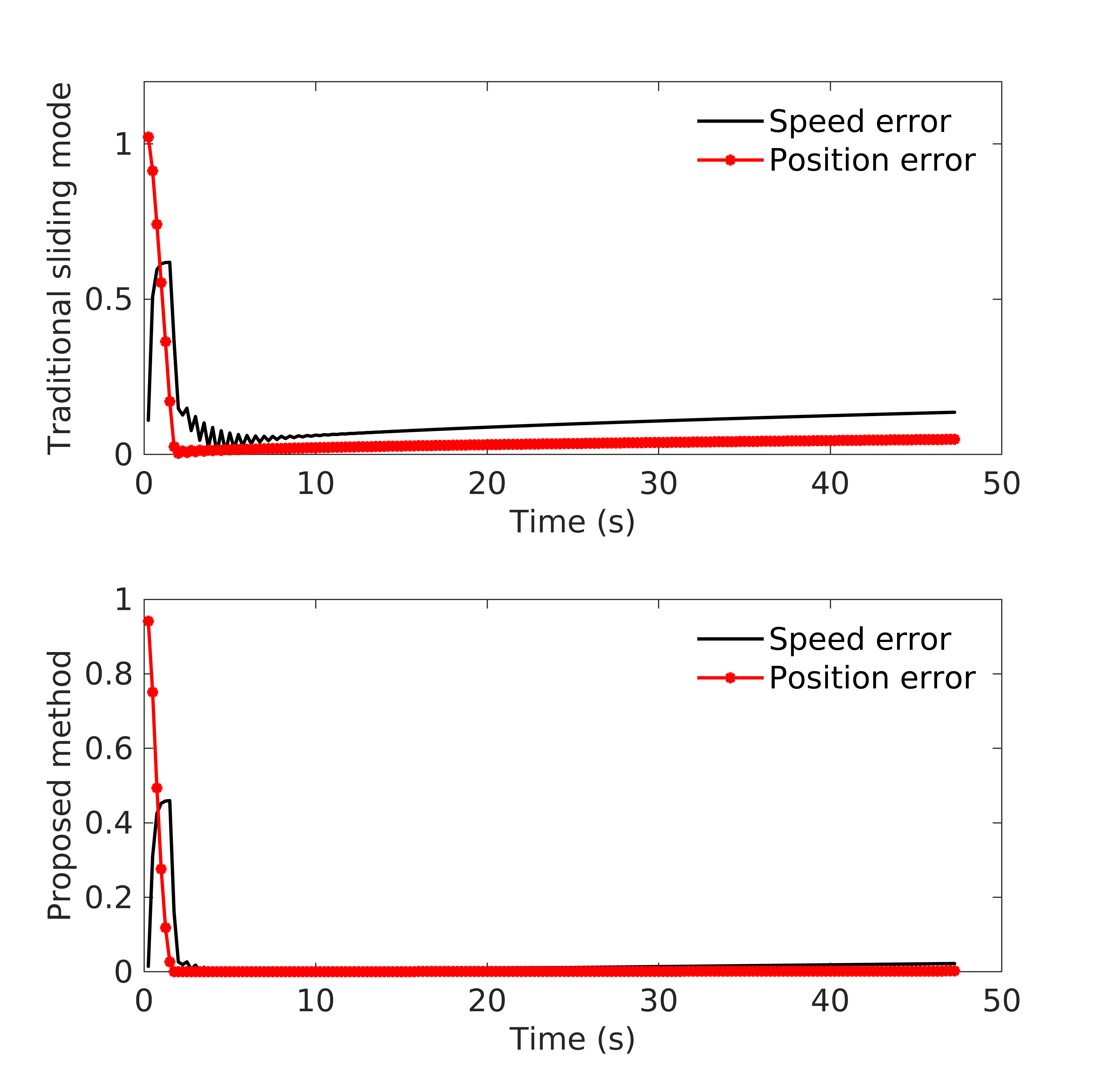
Fig. 13 shows the tracking error comparison of the traditional sliding mode method and the proposed method in the paper, taking the left follower as example, too. Note that the traditional method uses the first order sliding mode controller without the adaptive module proposed in this paper. Fig. 13 compares the tracking errors of the two kinds of methods in the $x$ axis direction. Tracking errors of the position and the speed of the AUV converge to a certain range. As the leader AUV moves, the tracking error increases and then decrease as the controller taking effect. The traditional method results jumping errors with obvious water flow influences, while the tracking error curves are smoother and smaller with the proposed method. In the same way, Fig. 13 shows the tracking error comparison in the $y$ axis direction and Fig. 13 shows the tracking error comparison in the $z$ axis direction. From these simulation results, we could find that the proposed method is effective to the formation control problem in the water flow environment.

References

- [1] J. J. Leonard and A. Bahr, Autonomous Underwater Vehicle Navigation. Cham: Springer International Publishing, 2016, ch. 14, pp. 341–358.
- [2] Z. Yu, J. Tao, J. Xiong, and S. X. Yang, “Design and analysis of path planning for robotic fish based on neural dynamics model,” International Journal of Robotics and Automation, vol. 36, no. 4, pp. 219–230, 2021.
- [3] R. Cui, S. S. Ge, B. V. E. How, and Y. S. Choo, “Leader-follower formation control of underactuated autonomous underwater vehicles,” Ocean Engineering, vol. 37, no. 17, pp. 1491–1502, 2010.
- [4] Y. Li, X. Li, D. Zhu, and S. X. Yang, “Self-competition leader-follower multi-auv formation control based on improved pso algorithm with energy consumption allocation,” International Journal of Robotics and Automation, vol. 37, no. 3, pp. 288–301, 2022.
- [5] W. Ren, “Consensus tracking under directed interaction topologies: Algorithms and experiments,” IEEE Transactions on Control Systems Technology, vol. 18, no. 1, pp. 230–237, Jan 2010.
- [6] B. Zhu, L. Xie, D. Han, X. Meng, and R. Teo, “A survey on recent progress in control of swarm systems,” Science China Information Sciences, vol. 60, no. 7, Jul. 2017.
- [7] W. Ren, “Consensus strategies for cooperative control of vehicle formations,” IET Control Theory Applications, vol. 1, no. 2, pp. 505–512, March 2007.
- [8] Y. Cao, W. Ren, and Y. Li, “Distributed discrete-time coordinated tracking with a time-varying reference state and limited communication,” Automatica, vol. 45, no. 5, pp. 1299–1305, 2009.
- [9] Y. Tian and C. Liu, “Consensus of multi-agent systems with diverse input and communication delays,” IEEE Transactions on Automatic Control, vol. 53, no. 9, pp. 2122–2128, Oct 2008.
- [10] P. Lin and Y. Jia, “Further results on decentralised coordination in networks of agents with second-order dynamics,” IET Control Theory Applications, vol. 3, no. 7, pp. 957–970, July 2009.
- [11] J. Wen, C. Wang, and G. Xie, “Asynchronous distributed event-triggered circle formation of multi-agent systems,” Neurocomputing, vol. 295, pp. 118–126, Jun. 2018.
- [12] X. Cai and M. d. Queiroz, “Adaptive Rigidity-Based Formation Control for Multirobotic Vehicles With Dynamics,” IEEE Transactions on Control Systems Technology, vol. 23, no. 1, pp. 389–396, Jan. 2015.
- [13] J. Wang, D. Cheng, and X. Hu, “Consensus of multi-agent linear dynamic systems,” Asian Journal of Control, vol. 10, no. 2, pp. 144–155, 2008.
- [14] Z. Li, Z. Duan, and G. Chen, “Dynamic consensus of linear multi-agent systems,” IET Control Theory Applications, vol. 5, no. 1, pp. 19–28, January 2011.
- [15] F. Giulietti, M. Innocenti, M. Napolitano, and L. Pollini, “Dynamic and control issues of formation flight,” Aerospace Science and Technology, vol. 9, no. 1, pp. 65–71, 2005.
- [16] Y. Yang, H. Modares, D. C. Wunsch, and Y. Yin, “Leader–-follower Output Synchronization of Linear Heterogeneous Systems With Active Leader Using Reinforcement Learning,” IEEE Transactions on Neural Networks and Learning Systems, vol. 29, no. 6, pp. 2139–2153, Jun. 2018.
- [17] W. Gan, D. Zhu, and S. Yang, “A speed jumping-free tracking controller with trajectory planner for unmanned underwater vehicle,” International Journal of Robotics and Automation, vol. 35, pp. 339–346, 01 2020.
- [18] C. Hao, Y. Wang, H. Wang, and Z. Zhou, “Model-free adaptive control for time-varying trajectory tracking of non-linear systems,” International Journal of Robotics and Automation, vol. 34, no. 1, pp. 71–77, 2019.
- [19] B. Qin, H. Yan, H. Zhang, Y. Wang, and S. X. Yang, “Enhanced reduced-order extended state observer for motion control of differential driven mobile robot,” IEEE Transactions on Cybernetics, pp. 1–12, 2021.
- [20] Y. Chang, H. Yan, W. Huang, R. Quan, and Y. Zhang, “A novel starting method with reactive power compensation for induction motors,” IET Power Electronics, vol. n/a, no. n/a, 2022. [Online]. Available: https://ietresearch.onlinelibrary.wiley.com/doi/abs/10.1049/pel2.12392
- [21] F. Fahimi, “Sliding-mode formation control for underactuated surface vessels,” IEEE Transactions on Robotics, vol. 23, no. 3, pp. 617–622, June 2007.
- [22] K. Liu, Y. Wu, J. Xu, Y. Wang, Z. Ge, and Y. Lu, “Fuzzy sliding mode control of 3-dof shoulder joint driven by pneumatic muscle actuators,” International Journal of Robotics and Automation, vol. 34, no. 1, pp. 38–45, 2019.
- [23] Y. Shtessel, I. Shkolnikov, and M. D.J. Brown, “A second-order smooth sliding mode control,” Asian Journal of Control, vol. 5, pp. 498–504, 12 2003.
- [24] C. Edwards and S. Spurgeon, Sliding Mode Control: Theory And Applications. Bristol: Taylor & Francis, 1998.
- [25] S. Soylu, B. J. Buckham, and R. P. Podhorodeski, “A chattering-free sliding-mode controller for underwater vehicles with fault-tolerant infinity-norm thrust allocation,” Ocean Engineering, vol. 35, no. 16, pp. 1647–1659, 2008.
- [26] G. Antonelli, F. Caccavale, S. Chiaverini, and G. Fusco, “A novel adaptive control law for underwater vehicles,” IEEE Transactions on Control Systems Technology, vol. 11, no. 2, pp. 221–232, March 2003.
- [27] B. Sun and D. Zhu, “A chattering-free sliding-mode control design and simulation of remotely operated vehicles,” in 2011 Chinese Control and Decision Conference (CCDC), May 2011, pp. 4173–4178.
- [28] L. Ma, “Cooperative target tracking in concentric formations,” International Journal of Robotics and Automation, vol. 36, pp. 1–14, 2021.
- [29] T. Salgado-Jimenez and B. Jouvencel, “Using a high order sliding modes for diving control a torpedo autonomous underwater vehicle,” in Oceans 2003. Celebrating the Past … Teaming Toward the Future (IEEE Cat. No.03CH37492), vol. 2, Sep. 2003, pp. 934–939.
- [30] J. Davila, L. Fridman, and A. Levant, “Second-order sliding-mode observer for mechanical systems,” IEEE Transactions on Automatic Control, vol. 50, no. 11, pp. 1785–1789, Nov 2005.
- [31] X. Li and D. Zhu, “Formation control of a group of AUVs using adaptive high order sliding mode controller,” in OCEANS 2016 - Shanghai. Shanghai, China: IEEE, Apr. 2016, pp. 1–6.
- [32] L. Kong, W. He, C. Yang, Z. Li, and C. Sun, “Adaptive fuzzy control for coordinated multiple robots with constraint using impedance learning,” IEEE Transactions on Cybernetics, vol. 49, no. 8, pp. 3052–3063, 2019.
- [33] J. Wang, C. Wang, Y. Wei, and C. Zhang, “Sliding mode based neural adaptive formation control of underactuated auvs with leader-follower strategy,” Applied Ocean Research, vol. 94, p. 101971, 2020.
- [34] C. Meng and X. Zhang, “Distributed leaderless formation control for multiple autonomous underwater vehicles based on adaptive nonsingular terminal sliding mode,” Applied Ocean Research, vol. 115, p. 102781, 2021. [Online]. Available: https://www.sciencedirect.com/science/article/pii/S0141118721002571
- [35] G. Antonelli, S. Chiaverini, N. Sarkar, and M. West, “Adaptive control of an autonomous underwater vehicle: experimental results on odin,” IEEE Transactions on Control Systems Technology, vol. 9, no. 5, pp. 756–765, Sep. 2001.
- [36] T. I. Fossen, Guidance and Control of Ocean Vehicles. Norway: John Wiley & Sons, 1994.
- [37] G. Antonelli, Underwater robots. Berlin: Springer, 2014.
- [38] S. P. Hou and C. C. Cheah, “Pd control scheme for formation control of multiple autonomous underwater vehicles,” in 2009 IEEE/ASME International Conference on Advanced Intelligent Mechatronics, July 2009, pp. 356–361.
- [39] E. P. Chassignet, H. E. Hurlburt, E. J. Metzger, O. M. Smedstad, and et al., “US GODAE: Global ocean prediction with the hybrid coordinate ocean model (HYCOM),” Oceanography, vol. 22, no. 2, pp. 64–75, 2009.
- [40] A. Alvarez, A. Caiti, and R. Onken, “Evolutionary path planning for autonomous underwater vehicles in a variable ocean,” IEEE Journal of Oceanic Engineering, vol. 29, no. 2, pp. 418–429, April 2004.
- [41] Levant and Arie, “Higher-order sliding modes, differentiation and output-feedback control,” International Journal of Control, vol. 76, no. 9-10, pp. 924–941, 2003.
- [42] A. Pisano and E. Usai, “Sliding mode control: A survey with applications in math,” Mathematics & Computers in Simulation, vol. 81, no. 5, pp. 954–979, 2011.
- [43] W. Gan, D. Zhu, and D. Ji, “QPSO-model predictive control-based approach to dynamic trajectory tracking control for unmanned underwater vehicles,” Ocean Engineering, vol. 158, pp. 208–220, Jun. 2018.
- [44] A. Sousa, L. Madureira, J. Coelho, J. Pinto, J. Pereira, J. Borges Sousa, and P. Dias, “Lauv: The man-portable autonomous underwater vehicle,” IFAC Proceedings Volumes, vol. 45, no. 5, pp. 268–274, 2012, 3rd IFAC Workshop on Navigation, Guidance and Control of Underwater Vehicles.
- [45] R. M. Jorge Estrela da Silva, Bruno Terra and J. B. de Sousa, “Modeling and simulation of the lauv autonomous underwater vehicle,” in 13th IEEE IFAC International Conference on Methods and Models in Automation and Robotics, Szczecin, Poland, Aug 2007, pp. 1–1.
- [46] M. M. M. Manhães, S. A. Scherer, M. Voss, L. R. Douat, and T. Rauschenbach, “Uuv simulator: A gazebo-based package for underwater intervention and multi-robot simulation,” in OCEANS 2016 MTS/IEEE Monterey, 2016, pp. 1–8.