Fluctuation-response theorem for Kullback-Leibler divergences to quantify causation

Consider two probability distributions $p(w)$ and $q(w)$ of a random variable $w$. The KL divergence from $q(w)$ to $p(w)$ is defined as

it is not symmetric in its arguments, and non-negative. Importantly, it is invariant under invertible transformations $w\rightarrow w^{\prime}$ [18], namely $D\left[p(w)\big{|}\big{|}q(w)\right]=D\left[p(w^{\prime})\big{|}\big{|}q(w^{\prime})\right]$.

Consider a stochastic system of $n$ variables evolving with ergodic Markovian dynamics. Our goal is to define a quantitative measure of causation, i.e., the influence that a variable $x$ exerts over the dynamics of another variable $y$. We want this definition to have both the invariance property of KL divergences, and the physical interpretation of a propagation of perturbations.

Since the dynamics is ergodic, and therefore stationary, it suffices to consider the stochastic variables $x_{0}\equiv x(t=0)$, $y_{0}\equiv y(t=0)$ at $t=0$, and a time interval $\tau$ later $y_{\tau}\equiv y(t=\tau)$. To avoid cluttered notation, we will implicitly assume that the current values of the remaining $n-2$ variables are absorbed into $y_{0}$, e.g., $p(y_{\tau}\big{|}y_{0})\equiv p(y_{\tau}\big{|}y_{0},z_{0})$. Conditioning on $z_{0}$ avoids confounding variables in $z$ to introduce spurious causal links between $x$ and $y$ [24].

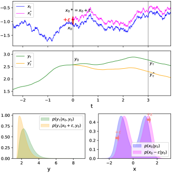
Let us consider the system at $t=0$ with steady-state distribution $p(x_{0},y_{0})$. We make an ideal measurement of its actual state $(x_{0},y_{0})$. Immediately after the measurement, we perturb the state by introducing a small displacement $\epsilon>0$ of the variable $x$, namely $x_{0}\Rightarrow x_{0}+\epsilon$. If the effect of this perturbation propagates to $y$, then it is reflected in the KL divergence from the natural to the perturbed prediction

which is a function of the local condition $(x_{0},y_{0})$ and the perturbation strength $\epsilon$. We name it local response divergence, and denote its ensemble average by $\left\langle d^{x\rightarrow y}_{\tau}(x_{0},y_{0},\epsilon)\right\rangle$.

The concept of causation, interpreted in the framework of fluctuation-response theory, is only meaningful with respect to an arrow of time. That means to postulate that the perturbation cannot have effects at past times

In writing the conditional probability $p\left(y_{\tau}\big{|}x_{0}+\epsilon,y_{0}\right)$, we implicitly assumed $p\left(x_{0}+\epsilon,y_{0}\right)>0$, meaning that the condition provoked by the perturbation is possible under the natural statistics. This implies that the response statistics can be predicted without actually perturbing the system, which is the main idea of fluctuation-response theory [19, 20, 21, 22].

The mean local response divergence $\left\langle d^{x\rightarrow y}_{\tau}(x_{0},y_{0},\epsilon)\right\rangle$, like any response function in fluctuation-response theory, is defined in relation to a perturbation, irrespective of how difficult it may be to perform this perturbation. Intuitively, we expect that it takes more effort to perturb those variables that fluctuate less. Therefore, we consider the KL divergence from the natural to the perturbed ensemble of conditions

to quantify the information-theoretic cost of perturbations, and call it perturbation divergence.

For example, for an underdamped Brownian particle, the perturbation divergence is equivalent to the average thermodynamic work required to perform an $\epsilon$ perturbation of its velocity, up to a factor being the temperature, see Supplementary Information (SI). For an equilibrium ensemble in a potential $U(x)$, with Boltzmann distribution $p(x)\sim\exp(-\beta U(x))$, the perturbation divergence is the average reversible work $c_{x}(\epsilon)=\beta\left\langle U(x+\epsilon)-U(x)\right\rangle$. Note that the definition of Eq. (4) is general, and can be applied to more abstract models where thermodynamic quantities are not clearly identified.

We introduce the information response as the ratio between mean local response divergence and perturbation divergence, in the limit of a small perturbation

We can interpret $\Gamma^{x\rightarrow y}_{\tau}$ as an information-theoretic linear response coefficient. This information response is our measure of $x\rightarrow y$ causation with respect to the timescale $\tau$, see Fig. 1. The time arrow requirement (Eq. (3)) implies $\Gamma^{x\rightarrow y}_{\tau}=0$ for $\tau<0$.

Introducing the local information response $\gamma^{x\rightarrow y}_{\tau}(x_{0},y_{0})\equiv\lim\limits_{\epsilon\rightarrow 0}d^{x\rightarrow y}_{\tau}(x_{0},y_{0},\epsilon)/c_{x}(\epsilon)$, we can equivalently write $\Gamma^{x\rightarrow y}_{\tau}=\left\langle\gamma^{x\rightarrow y}_{\tau}(x_{0},y_{0})\right\rangle$.

The information response in the form of Eq. (5) inherently relies on the concept of controlled perturbations. We can reformulate it in purely observational form, in the spirit of the fluctuation-response theorem [19, 20, 21, 22], provided $p(x_{0},y_{0},y_{\tau})$ is sufficiently smooth.

The one-parameter family $\{p(y_{\tau}\big{|}x_{0},y_{0})\}_{x_{0}}$ of probability densities parametrized by $x_{0}$ (for fixed $y_{0}$) can be equipped with a Riemannian metric having $d^{x\rightarrow y}_{\tau}(x_{0},y_{0},\epsilon)$ as squared line element. In fact, the leading order term in the Taylor expansion of a KL divergence between probabilities that differ only by a small perturbation of a parameter is of second order, with coefficients known as Fisher information [18, 25]. Explicitly, expanding the mean response divergence for $\tau>0$, we obtain

where we used the interventional causality requirement (Eq. (3)), and probability normalization. Similarly, for the perturbation divergence we have

Applying the Fisher information representation to the information response, we get for $\tau>0$

that is the fluctuation-response theorem for KL divergences. For generalizations and a discussion of the connection with the classical fluctuation-response theorem see [26] and SI text. Eq. (8) is the ratio of two second derivatives over the same physical variable $x_{0}$, and it can be regarded as an application of L’Hôpital’s rule to Eq. (5).

In general, Fisher information is not easily connected to Shannon entropy and mutual information [27]. Below, we show that for linear stochastic systems, the information response, which is a ratio of Fisher information (Eq. (8)), is equivalent to the transfer entropy, a conditional form of mutual information.

The most widely used measure of information flow is the conditional mutual information

which is generally called transfer entropy [13, 14, 15, 16, 17]. It is the average KL divergence from conditional independence of $x_{0}$ and $y_{\tau}$ given $y_{0}$.

The transfer entropy is used in nonequilibrium thermodynamics of measurement-feedback systems, where it is related to work extraction and dissipation through fluctuation theorems [28, 16, 29]; in data science, causal network reconstruction from time series is based on statistical significance tests for the presence of transfer entropy [24].

If uncertainty is measured by the Shannon entropy $S[p(x)]=-\int dx~{}p(x)\ln p(x)$, then the transfer entropy quantifies how much, on average, the uncertainty in predicting $y_{\tau}$ from $y_{0}$ decreases if we additionally get to know $x_{0}$, $T^{x\rightarrow y}_{\tau}=\left\langle S\left[p\left(y_{\tau}\big{|}y_{0}\right)\right]-S\left[p\left(y_{\tau}\big{|}x_{0},y_{0}\right)\right]\right\rangle$.

While the joint probability $p\left(x_{0},y_{0},y_{\tau}\right)$ contains all the physics of the interacting dynamics of $x$ and $y$, the description in terms of the scalar transfer entropy $T^{x\rightarrow y}_{\tau}$ represents a form of coarse-graining.

We introduce the local transfer entropy $t^{x\rightarrow y}_{\tau}(x_{0},y_{0})=D\left[p(y_{\tau}\big{|}x_{0},y_{0})\big{|}\big{|}p(y_{\tau}\big{|}y_{0})\right]$; thus for the (macroscopic) transfer entropy $T^{x\rightarrow y}_{\tau}=\left\langle t^{x\rightarrow y}_{\tau}(x_{0},y_{0})\right\rangle$.

We next show that $T^{x\rightarrow y}_{\tau}$ and $\Gamma^{x\rightarrow y}_{\tau}$ are intimately related for linear systems.

As example of application, we study the information response in Ornstein-Uhlenbeck (OU) processes [30], i.e., linear stochastic systems of the type

where $\left\langle\eta^{(i)}_{t}\eta^{(j)}_{t^{\prime}}\right\rangle=q_{ij}\delta(t-t^{\prime})$ is Gaussian white noise with symmetric and constant covariance matrix. For the system to be stationary, we require the eigenvalues of the interaction matrix $A_{ij}$ to have positive real part. For our setting, we identify $x\equiv\xi^{(i)}$ and $y\equiv\xi^{(j)}$ for some particular $(i,j)$, and $z\equiv\{\xi^{(k)}\}_{k=1,...,n}\backslash\{\xi^{(i)},\xi^{(j)}\}$ as the remaining variables. Here, probability densities are normal distributions, $p(y_{\tau}\big{|}x_{0},y_{0})=\mathcal{N}_{y_{\tau}}(\langle y_{\tau}\big{|}x_{0},y_{0}\rangle,\sigma^{2}_{y_{\tau}|x_{0},y_{0}})$, with mean $\langle y_{\tau}\big{|}x_{0},y_{0}\rangle$ and variance $\sigma^{2}_{y_{\tau}|x_{0},y_{0}}\equiv\langle y_{\tau}^{2}\big{|}x_{0},y_{0}\rangle-\langle y_{\tau}\big{|}x_{0},y_{0}\rangle^{2}$, and similarly for $p(y_{\tau}\big{|}y_{0})$ and $p(x_{0}\big{|}y_{0})$. Expectations depend linearly on the conditions, $\partial^{2}_{x_{0}}\langle y_{\tau}\big{|}x_{0},y_{0}\rangle=0$, and variances are independent of them, $\partial_{x_{0}}\sigma^{2}_{y_{\tau}|x_{0},y_{0}}=0$. Recall the implicit conditioning on the confounding variables $z_{0}$ through $y_{0}$.

Applying these Gaussian properties to Eq. (8), the information response becomes:

where $\partial_{x_{0}}\langle y_{\tau}\big{|}x_{0},y_{0}\rangle$ can be interpreted as the coefficient of $x_{0}$ in the linear regression for $y_{\tau}$ based on the predictors $(x_{0},y_{0})$, and $\sigma^{2}_{y_{\tau}|x_{0},y_{0}}$ as its error variance. The variance $\sigma^{2}_{x_{0}|y_{0}}$ quantifies the strength of the natural fluctuations of $x_{0}$ (variable to be perturbed) conditional on $y_{0}$ (other variables). In fact, the information-theoretic cost of the perturbation, $c_{x}(\epsilon)=\epsilon^{2}\sigma^{-2}_{x_{0}|y_{0}}+\mathcal{O}(\epsilon^{3})$, is higher if $x_{0}$ and $y_{0}$ are more correlated.

In linear systems, the transfer entropy is equivalent to Granger causality [31]

as can be seen by substituting the Gaussian expressions for $p(y_{\tau}\big{|}x_{0},y_{0})$ and $p(y_{\tau}\big{|}y_{0})$ into Eq. (9).

The decrease in uncertainty in adding the predictor $x_{0}$ to the linear regression of $y_{\tau}$ based on $y_{0}$ reads

see SI text. Comparing Eq. (11) with Eq. (12) and using Eq. (13), we obtain a non-trivial equivalence between information response and transfer entropy for OU processes,

Remarkably, despite the equivalence of the macroscopic quantities $\Gamma^{x\rightarrow y}_{\tau}$ and $T^{x\rightarrow y}_{\tau}$, the corresponding local quantities are markedly different, see Fig. 2.

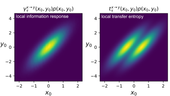
In Fig. 2, we show the local response divergence $\gamma^{x\rightarrow y}_{\tau}(x_{0},y_{0})$ and local transfer entropy $t^{x\rightarrow y}_{\tau}(x_{0},y_{0})$ for the hierarchical OU process of two variables

with $\left\langle\eta_{t}\eta_{t^{\prime}}\right\rangle=q\delta(t-t^{\prime})$, and parameters $\alpha$, $\beta>0$, $t_{R}>0$, $q>0$. This is possibly the simplest model of nonequilibrium stationary interacting dynamics with continuous variables [32]. However, the pattern of Fig. 2 is qualitatively the same for any linear OU process. In fact, the perturbation $x_{0}\Rightarrow x_{0}+\epsilon$ shifts the prediction $p(y_{\tau}\big{|}x_{0},y_{0})$ by the same amount on the $y$ axis, $\epsilon\partial_{x_{0}}\langle y_{\tau}\big{|}x_{0},y_{0}\rangle$, independently of the condition $(x_{0},y_{0})$, without affecting the variance $\sigma^{2}_{y_{\tau}|x_{0},y_{0}}$. Hence, $d^{x\rightarrow y}_{\tau}(x_{0},y_{0},\epsilon)$ is constant in space, and the local contribution only reflects the density $p(x_{0},y_{0})$, here a bivariate Gaussian. On the contrary, the KL divergence corresponding to the change of the prediction $p(y_{\tau}\big{|}y_{0})$ into $p(y_{\tau}\big{|}x_{0},y_{0})$ given by the knowledge of $x_{0}$, is strongly dependent on $(x_{0},y_{0})$. In fact, the local transfer entropy reads

see SI text. In particular, for likely values $x_{0}\approx\left\langle x_{0}\big{|}y_{0}\right\rangle$, the divergence $t^{x\rightarrow y}_{\tau}(x_{0},y_{0})$ is smaller compared to the unlikely situations $x_{0}\gg\left\langle x_{0}\big{|}y_{0}\right\rangle$ and $x_{0}\ll\left\langle x_{0}\big{|}y_{0}\right\rangle$. Thus, when multiplied by the steady-state density $p(x_{0},y_{0})$, $t^{x\rightarrow y}_{\tau}(x_{0},y_{0})$ attains a bimodal shape.

As a counter-example for the general validity of Eq. (14) for nonlinear systems, consider the following nonlinear Langevin equation for two variables

Numerical simulations (same parameters as for Eq. (15)) show that Eq. (14) is violated, see SI for details. Hence, in general, the transfer entropy is not easily connected to the information response.

Similar to the above, we can define an analogous information response at the ensemble level. From the same perturbation $x_{0}\Rightarrow x_{0}+\epsilon$, we consider the unconditional response divergence

i.e., we evaluate the response at the ensemble level, without knowledge of the measurement $(x_{0},y_{0})$,

In general $\widetilde{d^{x\rightarrow y}_{\tau}}(\epsilon)\neq\left\langle d^{x\rightarrow y}_{\tau}(x_{0},y_{0},\epsilon)\right\rangle$.

We define the ensemble information response as

where the second line, valid only for $\tau>0$, is the corresponding fluctuation-response theorem. A straightforward generalization to arbitrary perturbation profiles $\epsilon(x_{0},y_{0})$ is discussed in SI text. Note that we could write $\widetilde{d^{x\rightarrow y}_{\tau}}(\epsilon)$ through the Fisher information $\left\langle\partial^{2}_{\epsilon}\ln\left\langle p(y_{\tau}\big{|}x_{0}+\epsilon,y_{0})\right\rangle\right\rangle\big{|}_{\epsilon=0}$, but the partial derivative would be over the perturbation parameter $\epsilon$, and we found it more natural to consider the self-prediction quantity $\left\langle\left\langle\partial_{x_{0}}\ln p\left(y_{\tau}\big{|}x_{0},y_{0}\right)\big{|}y_{\tau}\right\rangle^{2}\right\rangle$. See SI text for technical details on expectation brakets.

In linear systems, the ensemble information response takes the form

where $I_{\tau}^{y,y}\equiv D\left[p(y_{0},y_{\tau})\big{|}\big{|}p(y_{0})p(y_{\tau})\right]$ is the mutual information between $y_{0}$ and $y_{\tau}$, and $I_{\tau}^{xy,y}=I_{\tau}^{y,y}+T^{x\rightarrow y}_{\tau}$ is the mutual information that the two predictors $(x_{0},y_{0})$ together have on the output $y_{\tau}$, see SI text.

From the nonnegativity of informations, we obtain the bound $0\leq\widetilde{\Gamma^{x\rightarrow y}_{\tau}}\leq 1$. We see that $\widetilde{\Gamma^{x\rightarrow y}_{\tau}}$ increases with the transfer entropy $T^{x\rightarrow y}_{\tau}$, and decreases with the autocorrelation $I_{\tau}^{y,y}$. Since $I_{\tau}^{y,y}$ diverges for $\tau\rightarrow 0$ in continuous processes, the perturbation on the $x$ ensemble takes a finite time to fully propagate its effect to the $y$ ensemble. Since time-lagged informations vanish for $\tau\rightarrow\infty$ in ergodic processes, ensembles relax asymptotically towards steady-state after a perturbation, and correspondingly the ensemble information response vanishes. This provides a trade-off shape for $\widetilde{\Gamma^{x\rightarrow y}_{\tau}}$ as a function of the timescale $\tau$. Note the asymptotics $\widetilde{\Gamma^{x\rightarrow y}_{\tau}}/\Gamma^{x\rightarrow y}_{\tau}\rightarrow 1$ for $\tau\rightarrow\infty$, also resulting from ergodicity.

In this Letter, we introduced a new measure of causation that has both the invariance properties required for an information-theoretic measure and the physical interpretation of a propagation of perturbations. It has the form of a linear response coefficient between Kullback-Leibler divergences, and it is based on the information-theoretic cost of perturbations. We would like to call it information response.

We study the behavior of the information response analytically in linear stochastic systems, and show that it reduces to the known transfer entropy in this case. This establishes a first connection between fluctuation-response theory and information flow, i.e., the two main perspectives to the problem of causation at present. Additionally, it provides a new relation between Fisher and mutual information.

We suggest our information response for the design of new quantitative causal inference methods [24]. Its practical estimation on time series, as it is normally the case for information-theoretic measures, depends on the learnability of probability distributions from a finite amount of data [33, 34].