FleXOR: Trainable Fractional Quantization
Abstract
Quantization based on the binary codes is gaining attention because each quantized bit can be directly utilized for computations without dequantization using look-up tables. Previous attempts, however, only allow for integer numbers of quantization bits, which ends up restricting the search space for compression ratio and accuracy. In this paper, we propose an encryption algorithm/architecture to compress quantized weights so as to achieve fractional numbers of bits per weight. Decryption during inference is implemented by digital XOR-gate networks added into the neural network model while XOR gates are described by utilizing for backward propagation to enable gradient calculations. We perform experiments using MNIST, CIFAR-10, and ImageNet to show that inserting XOR gates learns quantization/encrypted bit decisions through training and obtains high accuracy even for fractional sub 1-bit weights. As a result, our proposed method yields smaller size and higher model accuracy compared to binary neural networks.
1 Introduction
Deep Neural Networks (DNNs) demand a larger number of parameters and more computations to support various task descriptions all while adhering to ever-increasing model accuracy requirements. Because of abundant redundancy in DNN models [9, 5, 3], numerous model compression techniques are being studied to expedite the inference of DNNs [21, 17]. As a practical model compression scheme, parameter quantization is a popular choice because of the high compression ratio and regular formats after compression so as to enable full memory bandwidth utilization.
Quantization schemes based on binary codes are gaining increasing attention since quantized weights follow specific constraints to allow simpler computations during inference. Specifically, using the binary codes, a weight vector is represented as , where is the number of quantization bits, is a scaling factor , and each element of a vector is a binary . Then, a dot product with activations is conducted as , where is a full-precision activation and is the vector size. Note that the number of multiplications is reduced from to (expensive floating-point multipliers are less required for inference). Moreover, even though we do not discuss a new activation quantization method in this paper, if activations are also quantized by using binary codes, then most computations are replaced with bit-wise operations (using XNOR logic and population counts) [27, 22]. Consequently, even though representation space is constrained compared with quantization methods based on look-up tables, various inference accelerators can be designed to exploit the advantages of binary codes [22, 27]. Since a successful 1-bit weight quantization method has been demonstrated in BinaryConnect [3], advances in compression-aware training algorithms in the form of binary codes (e.g., binary weight networks [22] and LQ-Nets [29]) produce 1-3 bits for quantization while accuracy drop is modest or negligible. Fundamental investigations on DNN training mechanisms using fewer quantization bits have also been actively reported [19, 2].
Previously, binary-coding-based quantization has only permitted integer numbers of quantization bits, limiting the compression/accuracy trade-off search space, especially in the range of very low quantization bits. In this paper, we propose a flexible encryption algorithm/architecture (called “FleXOR”) to enable fractional sub 1-bit numbers to represent each weight while quantized bits are trained by gradient descent. Even though vector quantization is also a well-known scheme with a high compression ratio [24], we assume the form of binary codes. Note that the number of quantization bits can be different for each layer (e.g., [26]) to allow fractional quantization bits on average. FleXOR implies fractional quantization bits for each layer that can be quantized with a different number of bits.

To the best of our knowledge, our work is the first to explore model accuracy under 1 bit/weight when weights are quantized based on the binary codes. Figure 1 compares representations of weights to be stored in memory, converting method, and computation schemes of three quantization schemes. FleXOR maintains the advantages of binary-coding-based quantization (i.e., dequantization is not necessary for the computations) while quantized weights are further compressed by encryption. Note that since our major contribution is to enable fractional sub 1-bit weight quantization, for experiments, we selected models that have been previously quantized by ‘1’ bit/weight for comparisons on the model accuracy. As a result, unfortunately, the range of model selections is somewhat limited.
2 Encrypting Quantized Bits using XOR Gates

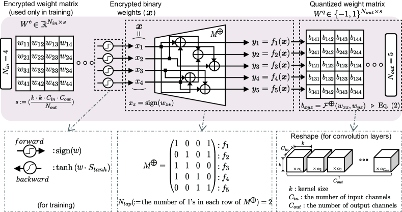
The main purpose of FleXOR is to compress quantized bits into encrypted bits that can be reconstructed by XOR gates as shown in Figure 2. Suppose that bits are to be compressed into bits (). The role of an XOR-gate network is to produce various -bit combinations using bits [15]. In other words, in order to maximize the chance of generating a desirable set of quantized bits, the encryption scheme is designed to seek a particular property where all possible outcomes through decryption are evenly distributed in space.
A linear Boolean function, , maps and has the form of where ( and indicates bit-wise modulo-2 addition. In Figure 2, six binary outputs are generated through six Boolean functions using four binary inputs. Let and be two such linear Boolean functions using . The Hamming distance between and is the number of inputs on which and differ, and defined as
| (1) |
where is the Hamming weight of a function and corresponds to the size of a set [13]. The Hamming distance is a well-known method to express non-linearity between two Boolean functions [13] and increased Hamming distance between a pair of two Boolean functions results in a variety of outputs produced by XOR gates. Increasing Hamming distance is a required feature for cryptography to derive complicated encryption structure such that inverting encrypted data becomes difficult. For digital communication, the Hamming distance between encoded signals is closely related to the amount of error correction possible.
FleXOR should be able to select the best out of possible outputs that are randomly selected from larger search space. Encryption performance of XOR gates is determined by the randomness of output candidates, and is enhanced by increasing Hamming distance that is achieved by larger (for a fixed compression ratio). Now, let be the number of 1’s in a row of . Another method to enhance encryption performance is to increase so as to increase the number of shuffles (through more XOR operations) using encrypted bits to generate quantized bits such that correlation between quantized bits is reduced.

In Figure 2, is represented as , or equivalently a vector denoting which inputs are selected. Concatenating such vectors, a XOR-gate network in Figure 2 can be described as a binary matrix (e.g., the second row of is and the third row is ). Then, decryption through XOR gates is simply represented as where and are the binary inputs and binary outputs of XOR gates, and addition is ‘XOR’ and multiplication is ‘AND’ (see Appendix for more details and examples).
Encrypted weight bits are stored in a 1-dimensional vector format and sliced into blocks of -bit size as shown in Figure 3. Then, the decryption of each slice is performed by an XOR-gate network that is shared by all slices (temporally- or spatially-shared). Depending on the quantization scheme and characteristics of layers, quantized bits may need to be scaled by a scaling factor and/or reshaped. Area and latency overhead induced by XOR gates are negligible as demonstrated in VLSI testing and parameter pruning works [25, 17, 1].
Since an XOR-gate network is shared by many weights (i.e., is fixed for all slices), it is difficult (if not impossible) to manually optimize an XOR-gate network. Hence, a random configuration is enough to fulfill the purpose of random number generation. In short, the XOR-gate network design is simple and straightforward.
3 FleXOR Training Algorithm for Quantization Bits Decision
Once the structure of XOR gates has been pre-determined and fixed to increase the Hamming distance of XOR outputs, we find quantized and encrypted bits by adding XOR gates into the model. In other words, we want an optimizer that understands the XOR-gate network structure so as to compute encrypted bits and scaling factors via gradient descent. For inference, we store binary encrypted weights (converted from real number encrypted weights) in memory and generate binary quantized weights through Boolean XOR operations. Activation quantization is not discussed in this paper to avoid the cases where the choice of activation quantization method affects the model accuracy.
Similar to the STE method introduced in [3], Boolean functions need to be described in a differentiable manner to obtain gradients in backward propagation. For two real number inputs and ( to be used as encrypted weights), the Boolean version of a XOR gate for forward propagation is described as (note that is replaced with )
| (2) |
For inference, we store and instead of and . On the other hand, a differentiable XOR gate for backward propagation is presented as
| (3) |
where is a scaling factor for FleXOR. Note that functions are widely used to approximate Heaviside step functions (i.e., if or , otherwise) in digital signal processing and can control the steepness. In [6, 16], is also suggested to approximate the STE function. In our work, on the other hand, is to proposed to make XOR operations trainable for ‘encryption.’ rather than ‘quantization.’ In the case of consecutive XOR operations, the order of inputs to be fed into XOR gates should not affect the computation of partial gradients for XOR inputs. Therefore, as a simple extension of Eq. (3), a differentiable XOR gate network with inputs can be described as
| (4) |
Then, a partial derivative of with respect to (an encrypted weight) is given as
| (5) |
Note that increasing is associated with more multiplications for each XOR-gate network output. From Eq. (5), thus, increasing may lead to the vanishing gradient problem since . To resolve this problem, we also consider a simplified alternative partial derivative expressed as
| (6) |
Compared to Eq. (5), approximation in Eq. (6) is obtained by replacing with . Eq. (6) shows that when we compute a partial derivative, all XOR inputs other than are assumed to be binary, i.e., the magnitude of a partial derivative is then only determined by . We use Eq. (6) in this paper to calculate custom gradients of encrypted weights due to fast training computations and convergence, and use Eq. (2) for forward propagation.
By training the whole network including FleXOR components using custom gradient computation methods described above, encrypted and quantized weights are obtained in a holistic manner. FleXOR operations for convolutional layers are described in Algorithm 1, where encrypted weights (inputs of an XOR-gate network) and quantized weights (outputs of an XOR-gate network) are and . We note that Algorithm 1 describes hardware operations (that are best implemented by ASIC or FPGA) rather than instructions to be operated by CPUs or GPUs.
We first verify the basic training principles of FleXOR using LeNet-5 on the MNIST dataset. LeNet-5 consists of two convolutional layers and two fully-connected layers (specifically, 32C5-MP2-64C5-MP2-512FC-10SoftMax), and each layer is accompanied by an XOR-gate network with binary inputs and binary outputs. The quantization scheme follows a 1-bit binary code with full-precision scaling factors that are shared across weights for the same output channel number (for conv layers) or output neurons (for FC layers). Encrypted weights are randomly initialized with . All scaling factors for quantization are initialized to be (note that if batch normalization layers are immediately followed, then scaling factors for quantization are redundant).


Using the Adam optimizer with an initial learning rate of 10-4 and batch size of 50 without dropout, Figure 4 shows training loss and test accuracy when , elements of are randomly filled with 1 or 0, and for two values of – and . Using the 1-bit internal quantization method and encryption scheme, one weight can be represented by bits. Hence, Figure 4 represents training results for 0.4, 0.6, and 0.8 bits per weight. Note that as for a randomly filled , increasing (and is determined correspondingly for the same compression ratio) increases the Hamming distance for a pair of any two rows of and, hence, offers the chance to produce more diversified outputs. Indeed, as shown in Figure 4, the results for =20 present improved test accuracy and less variation compared with =10. See Appendix for the distribution of encrypted weights at different training steps.
4 Practical FleXOR Training Techniques
In this section, we present practical training techniques for FleXOR using ResNet-32 [10] on the CIFAR-10 dataset [14]. We show compression results for ResNet-32 using fractional numbers as effective quantization bits, such as 0.4 and 1.2, that have not been available previously.
All layers, except the first and the last layers, are followed by FleXOR components sharing the same structure (thus, storage footprint of is ignorable). SGD optimizer is used with a momentum of 0.9 and a weight decay factor of . Initial learning rate is 0.1, which is decayed by 0.5 at the 150th and 175th epoch. As learning rate decays, is empirically multiplied by 2 to cancel out the effects of weight decay on encrypted weights. The batch size is 128 and initial scaling factors of are 0.2. ‘’ is the number of bits to represent binary codes for quantization. We provide some useful training insights below with relevant experimental results.
1) Use small (such as 2): Large can induce vanishing gradient problems in Eq. (5) or increased approximation error in Eq. (6). In practice, hence, FleXOR training with small converges well with high test accuracy. Studying a training algorithm to understand a complex XOR-gate network with large would be an interesting research topic that is beyond the scope of this work. Subsequently, we show experimental results using in the remainder of this paper.

| XOR Training Method | |||
| STE | Analog XOR | FleXOR | |
| Forward | |||
| Backward | Identity | ||
| XOR Output | Binary or | Binary or | |
2) Use ‘’ rather than STE for XOR: Since forward propagation for an XOR gate only needs a function, the STE method is also applicable to XOR-gate gradient calculations. Another alternative method to model an XOR gate is to use Eq. (3) for both forward and backward propagation as if the XOR is modeled in an analog manner (then, real number XOR outputs are quantized through STE). We compare three different XOR modeling schemes in Figure 5 with test accuracy measured when encrypted weights and XOR gates are converted to be binary for inference. FleXOR training method shows the best result because a) function for forward propagation enables estimating the impact of binary XOR computations on the loss function and b) for backward propagation approximates the Heaviside step function better compared to STE. Note that limited gradients from the function eliminate the need for weight clipping, which is often required for quantization-aware training schemes [3, 27].


3) Optimize : controls the smoothness of the function for near-zero inputs. Large employs large gradient for small inputs and, hence, results in well-clustered encrypted weight values as shown in Figure 6. Too large of a , however, hinders encrypted weights from being finely-tuned through training. For FleXOR, is a hyper-parameter to be optimized empirically.
4) Learning rate and warmup: Learning rate starts from 0 and linearly increases to reach the initial learning rate at a certain epoch as a warmup. Learning rate warmup is a heuristic scheme, but widely accepted to improve generalization capability mainly by avoiding large learning rate in the initial phase [11, 8]. Similarly, starts from 5, and linearly increases to 10 using the same warmup schedule of the learning rate.


5) Try various , , and : Using a warmup scheme for 100 epochs and learning rate decay by 50% at the 350th, 400th, and 450th epoch, Figure 7 presents test accuracy of ResNet-32 with various , , and . For , different configurations are constructed and then shared across all layers. Note that even for the 0.4bit/weight configuration (using , , and ), high accuracy close to 89% is achieved. 0.8bit/weight can be achieved by two different configurations (as shown on the right side of Figure 7) using (, , ) or (, , ). Interestingly, those two configurations show almost the same test accuracy, which implies that FleXOR is able to provide a linear relationship between the number of encrypted weights and model accuracy (regardless of internal configurations). In general, lowering reduces the number of computations with quantized weights.
| ResNet-20 | ResNet-32 | |||||
| 7 | ||||||
| FP | Compressed | Diff. | FP | Compressed | Diff. | |
| BWN (1 bit) | 92.68% | 87.44% | -5.24 | 93.40% | 89.49% | -4.51 |
| BinaryRelax (1 bit) | 92.68% | 87.82% | -4.86 | 93.40% | 90.65% | -2.80 |
| LQ-Net (1 bit) | 92.10% | 90.10% | -1.90 | - | - | - |
| DSQ (1 bit) | 90.70% | 90.24% | -0.56 | - | - | - |
| FleXOR (1.0 bit) | 91.87% | 90.44% | -1.47 | 92.33% | 91.36% | -0.97 |
| FleXOR (0.8 bit) | 89.91% | -1.90 | 91.20% | -1.13 | ||
| FleXOR (0.6 bit) | 89.16% | -2.71 | 90.43% | -1.90 | ||
| FleXOR (0.4 bit) | 88.23% | -3.64 | 89.61% | -2.72 | ||
We compare quantization results of ResNet-20 and ResNet-32 on CIFAR-10 using different compression schemes in Table 1 (with full-precision activation). BWN [22], BinaryRelax [28], and LQ-Net [29] propose different training algorithms for the same quantization scheme (i.e., binary codes). The main idea of these methods is to minimize quantization error and to obtain gradients from full-precision weights while the loss function is aware of quantization. Because all of the quantization schemes in Table 1 uses and binary codes, the amount of computations using quantized weights is the same. FleXOR, however, allows reduced memory footprint and bandwidth which are critical for energy-efficient inference designs [9, 1].
Note that even though achieving the best accuracy for 1.0 bit/weight is not the main purpose of FleXOR (e.g., XOR gate may be redundant for ), FleXOR shows the minimum accuracy drop for ResNet-20 and ResNet-32 as shown in Table 1. It would be an exciting research topic to study the distribution of the optimal number of quantization bits for each weight. We believe that such distribution would be wide and some weights require >1b while numerous weights need <1b because 1) increasing and allows such distributions to be wider and enhances model accuracy even for the same compression ratio and 2) as shown in Table 1, model accuracy of 1-bit quantization with FleXOR is higher than other quantization schemes that do not include encoding schemes.
| (Bits/Weight) | Average Bits/Weight | Accuracy | ||||
| Layer 2–7 (13.5k params) | Layer 8–13 (45k params) | Layer 14–19 (180k params) | ||||
| Fixed to be 12 (0.60) | 0.60 | 89.16% | ||||
| 19 (0.95) | 19 (0.95) | 8 (0.40) | 0.53 | 89.23% (+0.07) | ||
| 16 (0.80) | 16 (0.80) | 8 (0.40) | 0.50 | 89.19% (+0.03) | ||
| 19 (0.95) | 16 (0.80) | 7 (0.35) | 0.47 | 89.29% (+0.13) | ||
While binary neural networks allow only 1-bit quantization as the minimum, FleXOR can assign any fractional quantization bits (less than 1) to different layers. Such a property is especially useful when some layers exhibit high redundancy and relatively less importance such that very low number of quantization bits do not degrade accuracy noticeably [4, 26]. To demonstrate mixed-precision quantization (with all less than 1-bit) enabled by FleXOR, we conduct experiments with ResNet-20 on CIFAR-10 while employing three different XOR-gate structures (i.e. multiple configurations of are provided to different layer groups.). Table 2 shows that FleXOR with differently optimized for each layer group can achieve a higher compression ratio with a smaller storage footprint compared to the case of FleXOR associated with just one common configuration for all layers. When is fixed to be 20 for all layers, due to the varied importance of each group, small is allowed for the third group (of layers with a large number of parameters) while relatively large is selected for small layers. Compared to the case of =12 for all layers (with 0.6 bits/weights), adaptively chosen sets (i.e., 19 for layer 2-7, 16 for layer 8-13, and 7 for layer 14-19) yield higher accuracy (by 0.13%) and smaller bits/weights (by 0.13 bits/weights). As such, FleXOR facilitates a fine-grained exploration of optimal quantization bit search (given as fractional numbers determined by , , and ) that has not been available in the previous binary-coding-based quantization methods.
5 Experimental Results on ImageNet
In order to show that FleXOR principles can be extended to larger models, we choose ResNet-18 on ImageNet [23]. We use SGD optimizer with a momentum of 0.9 and an initial learning rate of 0.1. Batch size is 128, weight decay factor is , and is 10. Learning rate is reduced by half at the 70th, 100th, and 130th. For warmup, during the initial ten epochs, and learning rate increase linearly from 5 and 0.0, respectively, to initial values.
| Methods | Bits/Weight | Top-1 | Top-5 | Storage Saving |
| Full Precision [10] | 32 | 69.6% | 89.2% | 1 |
| BWN [22] | 1 | 60.8% | 83.0% | |
| ABC-Net [20] | 1 | 62.8% | 84.4% | |
| BinaryRelax [28] | 1 | 63.2% | 85.1% | |
| DSQ [7] | 1 | 63.7% | - | |
| FleXOR () | 0.8 | 63.8% | 84.8% | |
| 0.63 (mixed)111To 4 groups of 33 conv layers in ResNet-18 (except the first conv layer connected to the inputs), we assign 0.9, 0.8, 0.7, and 0.6 bits/weight, respectively. To the remaining 11 conv layers (performing downsampling), we assign 0.95, 0.9, and 0.8 bits/weight, respectively. | 63.3% | 84.5% | ||
| 0.6 | 62.0% | 83.7% | ||

Figure 8 depicts the test accuracy of ResNet-18 on ImageNet when (, and ) and (, and ). Refer to Appendix for more results with . Table 3 shows the comparison on model accuracy of ResNet-18 when weights are compressed by quantization (and additional encryption by FleXOR) while activations maintain full precision. Training ResNet-18 including FleXOR components is successfully performed. In Table 3, BinaryRelax and BWN do not modify the underlying model architecture, while ABC-Net introduces a new block structure of the convolution for quantized network designs. FleXOR achieves the best top-1 accuracy even with only 0.8bit/weight and demonstrates improved model accuracy as the number of bits per weight increases.
We acknowledge that there are numerous other methods to reduce the neural networks in size. For example, low-rank approximation and parameter pruning could be additionally performed to reduce the size further. We believe that such methods are orthogonal to our proposed method.
6 Conclusion
This paper proposes an encryption algorithm/architecture, FleXOR, as a framework to further compress quantized weights. Encryption is designed to produce more outputs than inputs by increasing the Hamming distance of output functions when output functions are linear functions of inputs. Output functions are implemented as a combination of XOR gates that are included in the model to find encrypted and quantized weights through gradient descent while using the function for backward propagation. FleXOR enables fractional numbers of bits for weights and, thus, much wider trade-offs between weight storage and model accuracy. Experimental results show that ResNet on CIFAR-10 and ImageNet can be represented by sub 1-bit/weight compression with high accuracy.
Broader Impact
Due to rapid advances in developing neural networks of higher model accuracy and increasingly complicated tasks to be supported, the size of DNNs is becoming exponentially larger. Our work facilitates the deployment of large DNN applications in various forms including mobile devices because of the powerful model compression ratio. As for positive perspectives, hence, a huge amount of energy consumption to run model inferences can be saved by our proposed quantization and encryption techniques. Also, a lot of computing systems that are based on binary neural network forms can improve model accuracy. We expect that lots of useful DNN models would be available for devices of low cost. On the other hand, some common concerns on DNNs such as privacy breaching and heavy surveillance can be worsened by DNN devices that are more available economically by using our proposed techniques.
Acknowledgments
We would like to thank the anonymous reviewers for their valuable comments on our manuscript.
References
- Ahn et al. [2019] D. Ahn, D. Lee, T. Kim, and J.-J. Kim. Double Viterbi: Weight encoding for high compression ratio and fast on-chip reconstruction for deep neural network. In International Conference on Learning Representations (ICLR), 2019.
- Choi et al. [2017] Y. Choi, M. El-Khamy, and J. Lee. Towards the limit of network quantization. In International Conference on Learning Representations (ICLR), 2017.
- Courbariaux et al. [2015] M. Courbariaux, Y. Bengio, and J.-P. David. BinaryConnect: Training deep neural networks with binary weights during propagations. In Advances in Neural Information Processing Systems, pages 3123–3131, 2015.
- Dong et al. [2019] Z. Dong, Z. Yao, A. Gholami, M. W. Mahoney, and K. Keutzer. Hawq: Hessian aware quantization of neural networks with mixed-precision. In Proceedings of the IEEE International Conference on Computer Vision, pages 293–302, 2019.
- Frankle and Carbin [2019] J. Frankle and M. Carbin. The lottery ticket hypothesis: Finding sparse, trainable neural networks. In International Conference on Learning Representations (ICLR), 2019.
- Gong et al. [2019a] R. Gong, X. Liu, S. Jiang, T. Li, P. Hu, J. Lin, F. Yu, and J. Yan. Differentiable soft quantization: Bridging full-precision and low-bit neural networks. arXiv:1908.05033, 2019a.
- Gong et al. [2019b] R. Gong, X. Liu, S. Jiang, T. Li, P. Hu, J. Lin, F. Yu, and J. Yan. Differentiable soft quantization: Bridging full-precision and low-bit neural networks. In Proceedings of the IEEE International Conference on Computer Vision, pages 4852–4861, 2019b.
- Gotmare et al. [2019] A. Gotmare, N. S. Keskar, C. Xiong, and R. Socher. A closer look at deep learning heuristics: Learning rate restarts, warmup and distillation. In International Conference on Learning Representations (ICLR), 2019.
- Han et al. [2016] S. Han, H. Mao, and W. J. Dally. Deep compression: Compressing deep neural networks with pruning, trained quantization and Huffman coding. In International Conference on Learning Representations (ICLR), 2016.
- He et al. [2016] K. He, X. Zhang, S. Ren, and J. Sun. Deep residual learning for image recognition. 2016 IEEE Conference on Computer Vision and Pattern Recognition (CVPR), pages 770–778, 2016.
- He et al. [2018] T. He, Z. Zhang, H. Zhang, Z. Zhang, J. Xie, and M. Li. Bag of tricks to train convolutional neural networks for image classification. In The IEEE Conference on Computer Vision and Pattern Recognition (CVPR), 2018.
- Jung et al. [2019] S. Jung, C. Son, S. Lee, J. Son, J.-J. Han, Y. Kwak, S. J. Hwang, and C. Choi. Learning to quantize deep networks by optimizing quantization intervals with task loss. In Proceedings of the IEEE Conference on Computer Vision and Pattern Recognition, pages 4350–4359, 2019.
- Kahn et al. [1988] J. Kahn, G. Kalai, and N. Linial. The influence of variables on boolean functions. In Proceedings of the 29th Annual Symposium on Foundations of Computer Science, SFCS ’88, pages 68–80, 1988.
- Krizhevsky et al. [2009] A. Krizhevsky, G. Hinton, et al. Learning multiple layers of features from tiny images. Technical report, Citeseer, 2009.
- Kwon et al. [2020] S. J. Kwon, D. Lee, B. Kim, P. Kapoor, B. Park, and G.-Y. Wei. Structured compression by weight encryption for unstructured pruning and quantization. In Proceedings of the IEEE/CVF Conference on Computer Vision and Pattern Recognition, pages 1909–1918, 2020.
- Lahoud et al. [2019] F. Lahoud, R. Achanta, P. Márquez-Neila, and S. Süsstrunk. Self-binarizing networks. arXiv:1902.00730, 2019.
- Lee et al. [2018] D. Lee, D. Ahn, T. Kim, P. I. Chuang, and J.-J. Kim. Viterbi-based pruning for sparse matrix with fixed and high index compression ratio. In International Conference on Learning Representations (ICLR), 2018.
- Li and Liu [2016] F. Li and B. Liu. Ternary weight networks. arXiv:1605.04711, 2016.
- Li et al. [2017] H. Li, S. De, Z. Xu, C. Studer, H. Samet, and T. Goldstein. Training quantized nets: A deeper understanding. In Advances in Neural Information Processing Systems, pages 5813–5823, 2017.
- Lin et al. [2017] X. Lin, C. Zhao, and W. Pan. Towards accurate binary convolutional neural network. In Advances in Neural Information Processing Systems, pages 345–353, 2017.
- Polino et al. [2018] A. Polino, R. Pascanu, and D. Alistarh. Model compression via distillation and quantization. In International Conference on Learning Representations (ICLR), 2018.
- Rastegari et al. [2016] M. Rastegari, V. Ordonez, J. Redmon, and A. Farhadi. XNOR-Net: Imagenet classification using binary convolutional neural networks. In ECCV, 2016.
- Russakovsky et al. [2015] O. Russakovsky, J. Deng, H. Su, J. Krause, S. Satheesh, S. Ma, Z. Huang, A. Karpathy, A. Khosla, M. Bernstein, A. C. Berg, and L. Fei-Fei. ImageNet Large Scale Visual Recognition Challenge. International Journal of Computer Vision (IJCV), 115(3):211–252, 2015. doi: 10.1007/s11263-015-0816-y.
- Stock et al. [2019] P. Stock, A. Joulin, R. Gribonval, B. Graham, and H. Jégou. And the bit goes down: Revisiting the quantization of neural networks. arXiv:1907.05686, 2019.
- Touba [2006] N. A. Touba. Survey of test vector compression techniques. IEEE Design & Test of Computers, 23:294–303, 2006.
- Wang et al. [2019] K. Wang, Z. Liu, Y. Lin, J. Lin, and S. Han. Haq: Hardware-aware automated quantization with mixed precision. In Proceedings of the IEEE Conference on Computer Vision and Pattern Recognition, pages 8612–8620, 2019.
- Xu et al. [2018] C. Xu, J. Yao, Z. Lin, W. Ou, Y. Cao, Z. Wang, and H. Zha. Alternating multi-bit quantization for recurrent neural networks. In International Conference on Learning Representations (ICLR), 2018.
- Yin et al. [2018] P. Yin, S. Zhang, J. Lyu, S. Osher, Y. Qi, and J. Xin. Binaryrelax: A relaxation approach for training deep neural networks with quantized weights. SIAM Journal on Imaging Sciences, 11(4):2205–2223, 2018.
- Zhang et al. [2018] D. Zhang, J. Yang, D. Ye, and G. Hua. Lq-nets: Learned quantization for highly accurate and compact deep neural networks. In Proceedings of the European Conference on Computer Vision (ECCV), pages 365–382, 2018.
- Zhu et al. [2017] C. Zhu, S. Han, H. Mao, and W. J. Dally. Trained ternary quantization. In International Conference on Learning Representations (ICLR), 2017.
Appendix A Example of a XOR-gate Network Structure Representation
In Figure 2, outputs of an XOR-gate network are given as
Equivalently, the same structure as above can be represented in a matrix as
| (7) |
Note that elements of are matched with coefficients of . For two vectors and , the following equation holds:
| (8) |
where element-wise addition and multiplication are performed by ‘XOR’ and ‘AND’ function, respectively. In Eq. (7), (i.e., the number of ‘1’s in a row) is 2 or 3.
Appendix B Supplementary Data for Basic FleXOR Training Principles
A Boolean XOR gate can be modeled as if is replaced with as shown in Table 4.
In Eq. (7), forward propagation for is expressed as
| (9) |
while partial derivative of with respect to is given as (not derived from Eq. (9))
| (10) |
or as
| (11) |


As shown in Figure 9, large yields sharp transitions for near-zero inputs. Such a sharp approximation of the Heaviside step function produces large gradient values for small inputs and encourages encrypted weights to be separated into negative or positive values. Too large , however, has the same issues of a too-large learning rate.


Figure 12 presents training loss and test accuracy when and is 10 or 20. Compared with Figure 5, presents improved accuracy for the cases of high compression configurations (e.g., and ). We use for CIFAR-10 and ImageNet, since low avoids gradient vanishing problems or high approximation errors in Eq.(5) or Eq.(6).

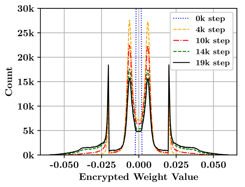
Figure 13 plots the distribution of encrypted weights at different training steps when each row of is randomly assigned with (i.e., is on average) or assigned with only two 1’s (=2). Due to gradient calculations based on and high , encrypted weights tend to be clustered on the left or right (near-zero encrypted weights become less as increases) even without weight clipping.
Appendix C Supplementary Experimental Results of CIFAR-10 and ImageNet
In this section, we additionally provide various graphs and accuracy tables for ResNet models on CIFAR10 and ImageNet. We also present experimental results from wider hyper-parameters searches including with two separate configurations (with the same and for two matrices).


| Bits/Weight | ResNet-20 | ResNet-32 | Comp. Ratio | |||
| FP | 32 | 91.87% | Diff. | 92.33% | Diff. | 1.0x |
| =10, =10 | 1.0 | 90.21% | -1.66 | 91.40% | -0.93 | 29.95 |
| =9, =10 | 0.9 | 90.03% | -1.84 | 91.28% | -1.05 | 31.82 |
| =8, =10 | 0.8 | 89.73% | -2.14 | 90.96% | -1.37 | 35.32 |
| =7, =10 | 0.7 | 89.88% | -1.99 | 90.67% | -1.66 | 39.68 |
| =6, =10 | 0.6 | 89.21% | -2.66 | 90.41% | -1.92 | 45.27 |
| =5, =10 | 0.5 | 88.59% | -3.28 | 89.95% | -2.38 | 52.70 |
| ResNet-20 | ResNet-32 | |||||
| FP | Quant. | Diff. | FP | Quant. | Diff. | |
| TWN (ternary) | 92.68% | 88.65% | -4.03 | 93.40% | 90.94% | -2.46 |
| BinaryRelax (ternary) | 92.68% | 90.07% | -1.91 | 93.40% | 92.04% | -1.36 |
| TTQ (ternary) | 91.77% | 91.13% | -0.64 | 92.33% | 92.37% | +0.04 |
| LQ-Net (2 bit) | 92.10% | 91.80% | -0.30 | - | - | - |
| FleXOR(, ) | ||||||
| =20, 2.0 bit/weight | 91.87% | 91.38% | -0.49 | 92.33% | 92.25% | -0.08 |
| =18, 1.8 bit/weight | 91.00% | -0.87 | 92.27% | -0.06 | ||
| =16, 1.6 bit/weight | 90.88% | -0.99 | 92.11% | -0.22 | ||
| =14, 1.4 bit/weight | 90.90% | -0.97 | 92.02% | -0.31 | ||
| =12, 1.2 bit/weight | 90.56% | -1.31 | 91.62% | -0.71 | ||
| FleXOR(, ) | ||||||
| =10, 2.0 bit/weight | 91.87% | 91.19% | -0.68 | 92.33% | 92.61% | +0.28 |
| =9, 1.8 bit/weight | 91.44% | -0.43 | 92.09% | -0.24 | ||
| =8, 1.6 bit/weight | 91.10% | -0.77 | 92.08% | -0.25 | ||
| =7, 1.4 bit/weight | 90.94% | -0.93 | 91.74% | -0.59 | ||
| =6, 1.2 bit/weight | 90.56% | -1.31 | 91.37% | -0.96 | ||
| Methods | Bits/Weight | Top-1 | Top-5 |
| Full Precision [10] | 32 | 69.6% | 89.2% |
| TWN [18] | ternary | 61.8% | 84.2% |
| ABC-Net [20] | 2 | 63.7% | 85.2% |
| BinaryRelax [28] | ternary | 66.5% | 87.3% |
| TTQ(1.5 Wide) [30] | ternary | 66.6% | 87.2% |
| LQ-net [29] | 2 | 68.0% | 88.0% |
| QIL [12] | 2 | 68.1% | 88.3% |
| FleXOR (, ) | 1.6 (0.82) | 66.2% | 86.7% |
| 1.2 (0.62) | 65.4% | 86.0% | |
| 0.8 (0.42) | 63.8% | 85.0% | |