\stackMath

Flexibility of Two-Dimensional Euler Flows with Integrable Vorticity

Elia Bruè¹¹1Department of Decision Sciences, Università Bocconi, Milano, Italy. Email: [email protected]. & Maria Colombo²²2EPFL, Station 8, CH-1015 Lausanne, Switzerland. Email: [email protected]. & Anuj Kumar³³3Department of Mathematics, University of California Berkeley, CA 94720, USA. Email: [email protected].

Abstract

We propose a new convex integration scheme in fluid mechanics, and we provide an application to the two-dimensional Euler equations. We prove the flexibility and nonuniqueness of $L^{\infty}L^{2}$ weak solutions with vorticity in $L^{\infty}L^{p}$ for some $p>1$ , surpassing for the first time the critical scaling of the standard convex integration technique.

To achieve this, we introduce several new ideas, including:

(i)

A new family of building blocks built from the Lamb-Chaplygin dipole.
(ii)

A new method to cancel the error based on time averages and non-periodic, spatially-anisotropic perturbations.

1 Introduction

We investigate the homogeneous incompressible Euler equations:

\begin{cases}\partial_{t}u+\mathop{div}\nolimits(u\otimes u)+\nabla p=0,\\ \mathop{div}\nolimits u=0\,,\end{cases}

(EU)

where $u$ represents the unknown velocity field and $p$ denotes the scalar pressure field. These equations are posed on the two-dimensional domain $\mathbb{T}^{2}=[-\pi,\pi]^{2}$ with periodic boundary conditions.

Our focus lies on weak solutions $u\in C_{t}L^{2}_{x}$ with vorticity $\omega:=\text{curl}\,u$ that is uniformly integrable, $\omega\in C_{t}L^{p}_{x}$ . The main result of this paper asserts that the system (EU) is flexible within this class, for small values of $p>1$ . A first example of flexibility is:

Theorem 1.1 (Flexibility).

There exists $p>1$ such that the following holds. For any divergence-free velocity fields $u_{\rm star},u_{\rm end}\in L^{2}(\mathbb{T}^{2})$ with zero mean, and any ${\varepsilon}>0$ , there exists a weak solution $u\in C([0,1];L^{2}(\mathbb{T}^{2}))$ to (EU) with $\omega\in C([0,1];L^{p}(\mathbb{T}^{2}))$ such that $\|u(\cdot,0)-u_{\rm star}\|_{L^{2}}\leq{\varepsilon}$ and $\|u(\cdot,1)-u_{\rm end}\|_{L^{2}}\leq{\varepsilon}$ .

An immediate consequence of Theorem 1.1 is that there exists a dense set of initial conditions $u_{\text{start}}\in L^{2}\cap W^{1,p}$ with zero mean, such that the Cauchy problem associated with (EU) admits non-conservative weak solutions $u\in C_{t}L^{2}_{x}$ with vorticity $\omega\in C_{t}L^{p}_{x}$ . To see this, it is enough to pick $u_{\text{start}}$ with much higher kinetic energy than $u_{\text{end}}$ .

Our construction is also able to produce non-uniqueness for the same set of wild initial conditions $u_{\text{start}}\in L^{2}\cap W^{1,p}$ .

Theorem 1.2 (Nonuniqueness).

There exists $p>1$ and a dense subset of divergence-free velocity fields $u_{\rm{start}}\in L^{2}(\mathbb{T}^{2})\cap W^{1,p}(\mathbb{T}^{2})$ with zero mean, such that (EU) admits infinitely many non-conservative weak solutions $u\in C([0,1];L^{2}(\mathbb{T}^{2}))$ with $\omega\in C([0,1];L^{p}(\mathbb{T}^{2}))$ satisfying $u(\cdot,0)=u_{\rm start}$ .

The weak solutions to (EU) constructed in this paper are built using a new convex integration scheme. It is not surprising that a small modification of our approach is able to establish the following variant of flexibility for (EU) in the class of $C_{t}L^{2}_{x}$ with solutions having $C_{t}L_{x}^{p}$ vorticity.

Theorem 1.3 (Time-Wise Compact Support).

There exists a non-trivial weak solution $u\in C(\mathbb{R};L^{2}(\mathbb{T}^{2}))$ to (EU) with compact support in time and $\omega\in L^{\infty}(\mathbb{R};L^{p}(\mathbb{T}^{2}))$ for some $p>1$ .

As for many implementations of convex integration in fluid dynamics, a technical modification of the proof of Theorems 1.1 and 1.3 allows to obtain flexibility of solutions while prescribing their kinetic energy. We expect the following statement to follow by our arguments for some $p>1$ : for every positive smooth function $e:[0,1]\to\mathbb{R}$ there exists a weak solution $u\in C([0,1];L^{2}(\mathbb{T}^{2}))$ with $\omega\in C([0,1];L^{p}(\mathbb{T}^{2})$ such that

e(t)=\frac{1}{2}\int_{\mathbb{T}^{2}}|u(x,t)|^{2}\,dx\,,\quad t\in[0,1]\,.

(1.1)

The proof of such result should follow by modifying our iterative Proposition 3.1 below by including closeness to the energy profile, which in turn can be guaranteed with the idea introduced in [BDLSV19] of space-time cutoffs. However, given the required technical complications we prefer to not to purse this goal here.

1.1 Context and Motivations

A classical well-posedness result by Wolibner [Wol33] and Hölder [H3̈3] ensures that (EU) is well-posed in $C^{1,\alpha}$ for any $\alpha>0$ . The proof of this result is based on the fact that the vorticity $\omega=\text{curl}\,u$ of a solution to (EU) is transported by the velocity field $u$ when the latter is regular enough. More precisely, we have the following vorticity formulation of the Euler system:

\begin{cases}\partial_{t}\omega+(u\cdot\nabla)\omega=0\,,\\ u=\nabla^{\perp}\Delta^{-1}\omega\,,\end{cases}

(EUvor)

where the second equation, namely the Biot–Savart law, expresses the inverse of the curl operator on $\mathbb{T}^{2}$ . These well-posedness results are in stark contrast to the three-dimensional case, where Elgindi [Elg21] proved the formation of finite-time singularities due to vortex stretching. In two dimensions, the borderline case $u\in C^{1}$ is more delicate. In this class, Bourgain and Li [BL15] and later Elgindi and Masmoudi [EM20] proved strong ill-posedness for the Euler equation (see also [CMZO24]).

The transport structure of (EUvor) suggests that $L^{p}$ norms of the vorticity are formally conserved for any $p\in[1,\infty]$ . For $p>1$ , this property was utilized in [DM87] to establish the existence of distributional solutions starting from an initial data with vorticity in $L^{p}$ . A similar existence result is significantly more difficult for $p=1$ , and it was demonstrated by Delort [Del91] (see also [EM94, Maj93, VW93]), extending the existence theory to initial vorticities in $H^{-1}$ (where this latter condition ensures the finiteness of the energy) whose positive (or negative) part is absolutely continuous.

1.1.1 Uniqueness and Yudovich Class

The class of weak solutions with uniformly bounded vorticity holds a special significance in the well-posedness theory of the 2D-Euler equations. According to the classical result by Yudovich [Yud62, Yud63] (see also the proof in [Loe06] and generalizations [Vis99, CS]), it is stated that for any initial data $\omega_{0}\in L^{\infty}$ , there exists a unique solution $\omega\in L^{\infty}_{t}L^{\infty}_{x}$ to (EUvor) originating from $\omega_{0}$ . The insight behind Yudovich’s uniqueness result is that a bounded vorticity yields an almost Lipschitz velocity field via the Biot-Savart law. Considering the transport structure of (EUvor), this almost Lipschitz regularity suffices to guarantee well-posedness.

A central question is whether Yudovich’s result extends to the class of weak solutions with vorticity in $L^{\infty}_{t}L^{p}_{x}$ for $p<\infty$ . In this framework, the fluid velocity $u\in L^{\infty}_{t}W^{1,p}_{x}$ is only Sobolev regular, and Yudovich’s Gronwall type argument breaks down. However, in view of the developments on the DiPerna–Lions theory [DL89, Amb04] dealing with passive scalar with Sobolev velocity fields, one might expect to prove some form of well-posedness for (EUvor) in this class.

Recent developments point in the direction of non-uniqueness, although none of them has fully solved the problem yet. Vishik [Visb, Visa], (see also [ABC⁺24]), has been able to demonstrate non-uniqueness within the class of $L^{\infty}_{t}L^{p}_{x}$ vorticity, with an additional degree of freedom: an external body force belonging to the integrability space $L^{1}_{t}L^{p}_{x}$ . The non-uniqueness takes the form of symmetry breaking, and its construction is based on the existence of an unstable vortex.

A second attempt has been pursued by Bressan and Shen [BS21], based on numerical experiments which exhibit the symmetry-breaking type of non-uniqueness observed by Vishik. Their work represents a preliminary step towards a computer-assisted proof.

In the framework of point vortex systems, Grotto and Pappalettera [GP22] have recently demonstrated that any configuration of $N$ initial point vortices is the singular limit of an evolution of $N+2$ point vortices. As a corollary, they managed to prove non-uniqueness for the “symmetrized” weak vorticity formulation (1.2) in the class of measure-valued vorticities. Literature on point vortex systems is extensive and challenging to summarize; we refer the reader to the monographs [MB02, MP94].

1.1.2 Convex Integration and Flexibility

The first flexibility results for the $2D$ Euler equations were obtained by Scheffer [Sch93], who constructed nontrivial weak solutions $u\in L^{2}_{t}L^{2}_{x}$ with compact support in space and time. The existence of infinitely many dissipative weak solutions to the Euler equations was first proven by Shnirelman in [Shn00], in the regularity class $L^{\infty}_{t}L^{2}_{x}$ .

The convex integration method in fluid dynamics was pioneered by De Lellis and Székelyhidi in the context of the Onsager conjecture [DLS09, DLS13]. These constructions, inspired by Muller and Sverak’s work on Lipschitz differential inclusions [Mv03], as well as Nash’s paradoxical constructions for the isometric embedding problem [Nas54], have led to a remarkable sequence of works including [BDLIS15, DS17, Buc15], culminating in the resolution of the flexibility part of the Onsager Conjecture by Isett [Ise18]. Further developments in the study of the Onsager conjecture can be found in [Cho13, CLJ12, BDLS16, Ise22, NV23, GR24]. We refer to the surveys [BV19a, BV21, DLS17, DLS19, DLS22] for a more complete history of the Onsager program.

A significant breakthrough in convex integration was achieved by Buckmaster and Vicol [BV19b], who introduced intermittency into the scheme. This innovation allows to treat the three-dimensional Navier-Stokes equations, which yields the first flexibility result for weak solutions. Since then, convex integration with intermittency has proven to be powerful and versatile, applicable to various problems [MS18, BCDL21, CL22, CL23, CL21, NV23, BMNV23, KGN23]. In [BC23], the first and second authors designed a convex integration scheme with intermittency to address the problem of uniqueness of the two-dimensional Euler equations (EU) with vorticity $\omega\in L^{\infty}_{t}L^{p}_{x}$ , in relation to Yudovich’s result. However, they could not reach the class of integrable vorticities, proving nonuniqueness in the class of weak solutions with $\omega\in L^{\infty}_{t}L^{1,\infty}_{x}$ , where $L^{1,\infty}$ is a Lorentz space. Subsequently, Buck and Modena [BM24b, BM24a] proved nonuniqueness and flexibility in the class of weak solutions with $\omega\in L^{\infty}_{t}H^{p}_{x}$ , where $H^{p}$ is the Hardy space with parameter $0<p<1$ . Remarkably, their solutions are also admissible. The first nonuniqueness result with $L^{p}$ initial vorticity in the class of admissible solutions was established by Mengual in [Men23]. All these developments have highlighted the limitations of classical convex integration constructions with intermittency in two dimensions. Due to an inherent obstruction arising from the mechanism used to cancel the error and the Sobolev embedding theorem, convex integration solutions cannot achieve $L^{1}$ integrability for the vorticity. For an explanation of this obstruction, we refer the reader to [BC23, Section 1.1].

Our main results, Theorem 1.1 and Theorem 1.3, represent the first convex integration constructions that overcome the inherent obstruction and achieve integrability of the vorticity beyond the $L^{1}$ space. This is due to a completely new design, which will be explained in the next sections.

1.1.3 Energy Conservation, Vanishing Viscosity, Turbulence

Energy-dissipating solutions to the Euler equations are crucial in the theory of turbulence, particularly in relation to the concepts of anomalous dissipation and the zeroth law of turbulence. In three dimensions, the celebrated conjecture by Onsager, now established as a theorem, states that weak solutions to the Euler equations belonging to the class $u\in C^{\alpha}_{x,t}$ conserve energy when $\alpha>\frac{1}{3}$ , but may dissipate energy when $\alpha<\frac{1}{3}$ . The critical threshold $\alpha=\frac{1}{3}$ is dimensionless. Recently, [GR24] constructed solutions $u\in C^{\alpha}_{x,t}$ to the two-dimensional Euler equations $\eqref{EU}$ that do not conserve energy for a given $\alpha<1/3$ .

The question of energy conservation is particularly meaningful in the context of weak solutions $u\in L^{\infty}_{t}L^{2}_{x}$ to (EU) with uniformly integrable vorticity $\omega\in L^{\infty}_{t}L^{p}_{x}$ . A natural conjecture, generalizing Onsager’s conjecture, is the following.

Conjecture 1.4 (Energy Conservation).

(i)

If $p\geq 3/2$ , any weak solution $u\in L^{\infty}_{t}L^{2}_{x}$ to (EU) with $\omega\in L^{\infty}_{t}L^{p}_{x}$ conserves the kinetic energy.
(ii)

If $p<\frac{3}{2}$ , there exist weak solutions $u\in L^{\infty}_{t}L^{2}_{x}$ to (EU) with $\omega\in L^{\infty}_{t}L^{p}_{x}$ that do not conserve the energy.

Energy conservation for $p\geq 3/2$ has already been established; see, for instance, [CCFS08], [CFLS16]. To the best of our knowledge, Theorem 1.1 is the first advancement in the direction of flexibility.

In two space dimensions, vanishing viscosity solutions are known to exhibit more rigid properties compared to generic weak solutions to (EU). Specifically, if the initial vorticity $\omega_{0}\in L^{p}$ of a vanishing viscosity solution is integrable in $L^{p}$ for some $p>1$ , the solution automatically conserves energy. See [CFLS16], [LMPP21], [RP24], and [CS15]. Notably, the solutions constructed in Theorem 1.1 cannot be vanishing viscosity solutions. To the best of the authors’ knowledge, these represent the first examples of weak solutions to (EU) with uniformly integrable vorticity $\omega\in L^{\infty}_{t}L^{p}_{x}$ that are not vanishing viscosity solutions. In contrast, Yudovich solutions are always vanishing viscosity [Mas07, CDE22, CCS21].

Remark 1.1 (Energy Conservation vs Nonuniqueness).

In the context of weak solutions $u\in L^{\infty}_{t}L^{2}_{x}$ to (EU) with uniformly integrable vorticity $\omega\in L^{\infty}_{t}L^{p}_{x}$ , nonuniqueness is expected for every $p<\infty$ , whereas energy conservation is expected for $p\geq\frac{3}{2}$ . This highlights the distinct nature of non-uniqueness and energy non-conservation.

The vorticity formulation (EUvor) for weak solutions $u\in L^{\infty}_{t}L^{2}_{x}$ to (EU) with $\omega\in L^{\infty}_{t}L^{p}_{x}$ makes distributional sense as soon as $p\geq\frac{4}{3}$ , since $u\cdot\omega\in L^{\infty}_{t}L^{1}_{x}$ within this range. Solutions constructed in Theorem 1.1 and Theorem 1.3 are not distributional solutions to (EUvor); however, they satisfy the so-called symmetrized weak vorticity formulation, dating back to the works of Delort and Schochet:

\int_{\mathbb{T}^{2}}\omega(x,t)\phi(x)\,dx-\int_{\mathbb{T}^{2}}\omega(x,0)\phi(x)\,dx=\int_{0}^{t}\int_{\mathbb{T}^{2}\times\mathbb{T}^{2}}H_{\phi}(x,y)\omega(x,s)\omega(y,s)\,dx\,dy

(1.2)

for every test function $\phi\in C^{\infty}(\mathbb{T}^{2})$ , where $H_{\phi}(x,y):=(\nabla\phi(x)-\nabla\phi(y))\cdot K(x,y)$ and $K(x,y)$ is the Biot-Savart kernel.

In the study of 2D turbulence, the concept of enstrophy defect plays an important role in connection with the enstrophy cascade [Eyi01]. This concept suggests that, in certain turbulent regimes, weak solutions to (EUvor) might not satisfy the local enstrophy balance; that is, integral quantities such as

\int\beta(\omega(x,t))\,dx\,,\quad\beta\in C_{c}^{\infty}(\mathbb{R})\,,

(1.3)

might not be conserved. The local enstrophy balance is closely connected with the so-called renormalization property: we say that $\omega\in L^{\infty}_{t}L^{p}_{x}$ is a renormalized solution to (EUvor) if

\partial_{t}\beta(\omega)+\mathop{div}\nolimits(u\beta(\omega))=0\,,\quad\text{for every $\beta\in C_{c}^{\infty}(\mathbb{R})$}\,.

(1.4)

Notice that the notion of renormalized solution to (EUvor) is meaningful for every $\omega\in L^{1}_{t}L^{p}_{x}$ with $p\geq 1$ . It was observed in [Eyi01] and further elaborated in [LFMNL06] that any $\omega\in L^{\infty}_{t}L^{p}_{x}$ with $p\geq 2$ is a renormalized solution to (EUvor), as a consequence of the DiPerna-Lions theory [DL89]. Moreover, Crippa and Spirito [CS15] have shown that vanishing viscosity solutions are renormalized for every $p\geq 1$ . In stark contrast, our Theorem 1.1 provides the first example of non-renormalized solutions to (EU) with vorticity $\omega\in L^{\infty}_{t}L^{p}_{x}$ for some $p>1$ .

In view of the recent result [BCK24], one might guess that the renormalization property holds for $p>\frac{3}{2}$ and might fail for $p<\frac{3}{2}$ . However, this is only a speculation, and we pose it as an open question.

Problem 1.5.

Find $p^{*}\geq 1$ such that any weak solution $u\in L^{\infty}_{t}L^{2}_{x}$ to (EU) with $\omega\in L^{\infty}_{t}L^{p}_{x}$ is renormalized (i.e., satisfies (1.4)) for $p>p^{*}$ , while there are non-renormalized solutions for $p<p^{*}$ .

To the best of the author’s knowledge, the most accurate estimate to date is $1+\frac{1}{6500}<p^{*}\leq 2$ .

1.2 A New Convex Integration Scheme

The main obstacle to achieve a two dimensional vorticity that is $L^{1}$ integrable in space is the homogeneous nature of the perturbations in convex integration schemes. Typically, these perturbations are periodic with a large wavelength $\lambda\gg 1$ , which makes them appear homogeneous at scales $r\gg 1/\lambda$ . From the embedding theorem of Nash [Nas54] and the foundational works of De Lellis and Székelyhidi [DLS09, DLS13], every convex integration scheme to date possess this characteristics.

Some form of heterogeneity of perturbation has been introduced in convex integration schemes with intermittency, starting from the work of Buckmaster and Vicol [BV19b]. In these schemes, the $\lambda$ -periodic structure is maintained, but the perturbations exhibit heterogeneity at a much smaller scale, $1/\mu\ll 1/\lambda$ , depending on the extent of the intermittency. However, at larger scales $r\gg 1/\lambda$ , the perturbation remains homogeneous, which mantains the obstruction to achieve uniform $L^{1}$ integrability for the vorticity.

In this paper, we overcome this hurdle by drawing inspiration from our recent work [BCK24] on the linear transport equation

\partial_{t}\rho+u\cdot\nabla\rho=0\,,\quad\,\mathop{div}\nolimits u=0\,.

(1.5)

with an incompressible velocity field $u\in L^{\infty}_{t}W^{1,p}_{x}$ and density $\rho\in L^{\infty}_{t}L^{r}_{x}$ , which lies within the framework of DiPerna–Lions theory [DL89].

In this context, the convex integration approach has been applied to produce nonuniqueness and flexibility for the Cauchy problem associated with (1.5). However, this method encounters similar obstructions as in the Euler setting and cannot achieve the sharp range of well-posedness recently obtained in our work [BCK24]. In this work, we introduce a novel linear construction that generates nonunique solutions to (1.5) beyond the range attainable by convex integration. The key feature enabling this is the spatial heterogeneity of both the density and the velocity field.

Inspired by this analogy, the first key idea we introduce in convex integration is to completely change the design of the perturbations by:

•

eliminating the $\lambda$ periodicity,
•

achieving truly heterogeneous perturbations at every scale.

Given the error cancellation mechanism in the convex integration method, which relies on the low-frequency interaction between highly oscillating perturbations, it seems impractical to use perturbations with the aforementioned characteristics. The key idea to overcome this challenge is to exploit the time variable to rebuild spatial oscillations through time averages.

At a qualitative level, the principal part of the perturbation will be concentrated in a single small moving region at any given time. This approach retains the intermittent structure while losing periodicity. As is standard in convex integration, the primary component of the perturbation must almost solve the Euler equations. Therefore, we introduce another key idea: a new family of building blocks constructed from the Lamb-Chaplygin dipole. These building blocks will incorporate several new features:

•

Variable speed: This is useful to rebuild the error at the previous step without employing slow functions. The latter are unnatural in our scheme since we no longer have fast and slow variables.
•

Variable support size: As the building blocks are almost Euler solutions with a constant $L^{2}$ norm, the scaling of the Euler equations forces a variable size of the support.

1.2.1 Overview

In this section, we present a more detailed description of the new convex integration scheme based on the qualitative features described above. As with any convex integration scheme, given a solution $u_{q}$ of the Euler–Reynolds system:

\partial_{t}u_{q}+\mathop{div}\nolimits(u_{q}\otimes u_{q})+\nabla p_{q}=\mathop{div}\nolimits(R_{q})\,,\quad\mathop{div}\nolimits u_{q}=0\,,

(1.6)

our goal is to produce a new velocity field $u_{q+1}=u_{q}+v_{q+1}$ , which solves the Euler–Reynolds system with a smaller error $R_{q+1}$ . As a first step we decompose $R_{q}$ into rank-one tensors:

\displaystyle-\mathop{div}\nolimits(R_{q})=\mathop{div}\nolimits\left(\sum_{i=1}^{4}a_{i}(x,t)\xi_{i}\otimes\xi_{i}\right)+\nabla P^{\,d},

(1.7)

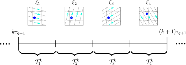
where the coefficients $a_{i}$ , $i\in\{1,2,3,4\}$ , are roughly the same size as $R_{q}$ , see Lemma 4.1. Our perturbation $v_{q+1}$ consists of only one building block moving in one of the $\xi_{i}$ directions at any given time. More precisely, it will be $\tau_{q+1}$ -periodic in time, and each interval of the form $[k\tau_{q+1},(k+1)\tau_{q+1}]$ , $k\in\mathbb{Z}$ , will be divided into four sub-intervals of equal length, each associated with a different direction $\xi_{i}$ . See Figure 1 below.

Refer to caption — Figure 1: shows the time interval $[k\tau_{q},(k+1)\tau_{q+1})$ which is further divided into four subintervals of equal length. The building block moves only in one of the direction $\xi_{i}$ , $i\in\{1,\dots,4\}$ , on a given subinterval.

For the sake of simplicity, in rest of the outline we assume that $R_{q}(x,t)=a(x,t)\xi\otimes\xi$ , where $\xi$ is a unit vector in a rationally dependent direction.

1.2.2 The New Building Blocks

Our building block is an almost exact solutions to the Euler system with source/sink term on $\mathbb{T}^{2}$ :

\begin{cases}\partial_{t}V+\mathop{div}\nolimits(V\otimes V)+\nabla P=S\frac{d}{dt}\,(\eta(t)r(t))+\mathop{div}\nolimits(F)\,,\\ \mathop{div}\nolimits(V)=0\,,\end{cases}

(1.8)

where $F\in C^{\infty}(\mathbb{T}^{2};\mathbb{R}^{2\times 2})$ is a small symmetric tensor that will be enclosed in the new error $R_{q+1}$ . The source/sink term $S\frac{d}{dt}\,(\eta(t)r(t))$ will be employed for the error cancellation through time-average, see the sketch in Section 1.2.3. Up to leading order, the velocity field has the following structure

\displaystyle V(x,t)=\eta(t)W_{r(t)}(x-x(t))\,,

(1.9)

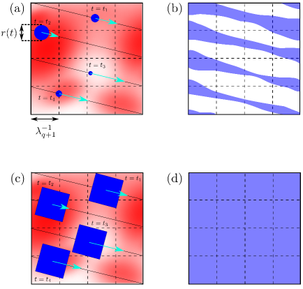
where $W_{r}(x)$ is the scaled core of the Lamb-Chaplygin dipole. The center of the core, $x(t)$ , travels at variable speed in the direction $\xi$ , according to the ODE:

x^{\prime}(t)=\frac{\eta(t)}{r(x(t))}\xi\,,\qquad\text{where}\qquad r(x)=r_{q+1}\overline{a}(x).

(1.10)

The function $r(x)$ is a space-dependent scale, proportional to a time average of $a(x,t)$ over intervals of length $\tau_{q+1}\ll 1$ . The parameter $r_{q+1}$ plays the role of the intermittency parameter in our construction. The function $\eta(t)$ is a smooth cut-off with support of size $\tau_{q+1}/4$ ; it serves to switch on and off the building block when swapping between the four directions. A fundamental feature of our construction is that $\xi$ is chosen such that the time period of $t\mapsto t\xi$ is large, $\lambda_{q+1}\gg 1$ . This parameter will play the role of the frequency in our construction.

Remark 1.2 (Comparison with Intermittent Jets).

Our new building blocks share some features with the intermittent jets introduced in [BCV21]. The main differences are:

•

Our new building blocks almost solve the Euler equations without the necessity of introducing time correctors.
•

The support and velocity of our building blocks vary.
•

The intermittent jets are shaped as ellipsoids in contrast with the more rounded design of ours.

The third point is the most problematic in our construction. The ellipsoidal design serves to control the size of the divergence but worsens the size of the vorticity. This loss is irremediable. Our scheme is able to reach $\omega\in L^{\infty}_{t}L^{1}_{x}$ using intermittent jets but cannot get past it.

1.2.3 Time Average and Error Cancellation

In this section, we illustrate the key calculation: how to reconstruct the error using time averages of the source/sink term $S\frac{d}{dt}(\eta(t)r(t))$ . For the sake of simplicity, let us assume that $S(x,t)=U(x-x(t))$ for some profile $U$ independent of time. We should stress that this assumption is not satisfied in our framework; however, we will demonstrate how to compensate for this deviation by introducing an auxiliary building block (see Section 4.7).

On every time interval $\mathcal{T}\subset[0,\infty]$ of length $\tau_{q+1}/4$ where $\eta(t)$ is supported, the time-average of the source term will be

\begin{split}\mathchoice{{\vbox{\hbox{$\textstyle-$ }}\kern-7.83337pt}}{{\vbox{\hbox{$\scriptstyle-$ }}\kern-5.90005pt}}{{\vbox{\hbox{$\scriptscriptstyle-$ }}\kern-4.75003pt}}{{\vbox{\hbox{$\scriptscriptstyle-$ }}\kern-4.25003pt}}\!\int_{\mathcal{T}}(\eta(t)r(t))^{\prime}U(x-x(t))\,dt&=-\mathchoice{{\vbox{\hbox{$\textstyle-$ }}\kern-7.83337pt}}{{\vbox{\hbox{$\scriptstyle-$ }}\kern-5.90005pt}}{{\vbox{\hbox{$\scriptscriptstyle-$ }}\kern-4.75003pt}}{{\vbox{\hbox{$\scriptscriptstyle-$ }}\kern-4.25003pt}}\!\int_{\mathcal{T}}\eta(t)r(t)\frac{d}{dt}U(x-x(t))\,dt\\ &=\mathchoice{{\vbox{\hbox{$\textstyle-$ }}\kern-7.83337pt}}{{\vbox{\hbox{$\scriptstyle-$ }}\kern-5.90005pt}}{{\vbox{\hbox{$\scriptscriptstyle-$ }}\kern-4.75003pt}}{{\vbox{\hbox{$\scriptscriptstyle-$ }}\kern-4.25003pt}}\!\int_{\mathcal{T}}\eta(t)^{2}(\xi\cdot\nabla)U(x-x(t))\,dt\\ &=\mathop{div}\nolimits\left(\mathchoice{{\vbox{\hbox{$\textstyle-$ }}\kern-7.83337pt}}{{\vbox{\hbox{$\scriptstyle-$ }}\kern-5.90005pt}}{{\vbox{\hbox{$\scriptscriptstyle-$ }}\kern-4.75003pt}}{{\vbox{\hbox{$\scriptscriptstyle-$ }}\kern-4.25003pt}}\!\int_{\mathcal{T}}\eta(t)^{2}U(x-x(t))\otimes\xi\,dt\right)\end{split}

(1.11)

We will carefully design $r(x)$ , $\eta(t)$ , and $U(x)$ to have

\mathchoice{{\vbox{\hbox{$\textstyle-$ }}\kern-7.83337pt}}{{\vbox{\hbox{$\scriptstyle-$ }}\kern-5.90005pt}}{{\vbox{\hbox{$\scriptscriptstyle-$ }}\kern-4.75003pt}}{{\vbox{\hbox{$\scriptscriptstyle-$ }}\kern-4.25003pt}}\!\int_{\mathcal{T}}\eta(t)^{2}U(x-x(t))\otimes\xi\,dt=a(x,t)\xi\otimes\xi+G

(1.12)

where $G\in C^{\infty}(\mathbb{T}^{2};\mathbb{R}^{2\times 2})$ is a new small error.

In other words, the time-mean of the source term is going to match exactly the error at the previous stage of the iteration. Thus, we only need to address the mean-free part of the source term. This is achieved by introducing an ad hoc time corrector $Q_{q+1}(x,t)$ ; see Section 4.8.

Acknowledgements:

EB would like to express gratitude for the financial support received from Bocconi University. MC is supported by the Swiss State Secretariat for Education, Research and lnnovation (SERI) under contract number MB22.00034 through the project TENSE.

2 Principal Building Block

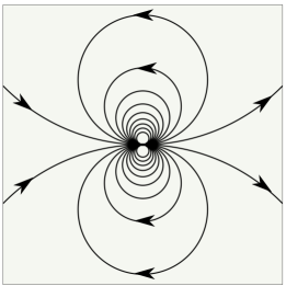
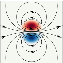
In this section, we construct the principal building block velocity field for our convex integration scheme. The main ingredient of our construction is the Lamb–Chaplygin dipole, an exact solution of the 2D Euler equation on $\mathbb{R}^{2}$ , which translates with constant velocity without undergoing deformation. The Lamb–Chaplygin dipole consists of two regions: a circular inner core of some fixed radius $r$ where the vorticity of opposite signs concentrate, and the complement of the core where the velocity field is irrotational. The Lamb–Chaplygin dipole can be understood as the desingularization of a potential flow known as the doublet flow.

We also introduce a cutoff and gluing procedure that enables us to relocate this dipole from $\mathbb{R}^{2}$ to $\mathbb{T}^{2}$ , while ensuring that it remains an approximate solution of the Euler equation. In addition to this relocation, we will consider a dipole on $\mathbb{T}^{2}$ whose core size $r$ expands or contracts as it translates. The effect of this is a source/sink term in the approximate Euler equation, which will ultimately be used to cancel the error term in the convex integration scheme.

2.1 Doublet Flow on $\mathbb{R}^{2}$

A doublet flow is a divergence-free potential flow on $\mathbb{R}^{2}\setminus\{0\}$ . We denote $x=(x_{1},x_{2})\in\mathbb{R}^{2}$ points in the Euclidean plane. In the complex notation, the potential $\widetilde{\Phi}$ and the stream function $\widetilde{\Psi}$ of the doublet flow are given by

\displaystyle\widetilde{\Phi}(x_{1},x_{2})+i\widetilde{\Psi}(x_{1},x_{2})\coloneqq-\frac{1}{z},\quad\text{where}\quad z=x_{1}+ix_{2}\,.

(2.1)

We define the velocity field $\widetilde{V}=(\widetilde{V}_{1},\widetilde{V}_{2})$ and the pressure as

\displaystyle\widetilde{V}\coloneqq\nabla^{\perp}\widetilde{\Psi}=\nabla\widetilde{\Phi}\,,\qquad\widetilde{P}\coloneqq\partial_{1}\widetilde{\Phi}-\frac{|\nabla\widetilde{\Phi}|^{2}}{2}.

(2.2)

where $\nabla^{\perp}=(-\partial_{2},\partial_{1})$ . From our definition, it is clear that $\widetilde{V}_{1}(x_{1},x_{2})-i\widetilde{V}_{2}(x_{1},x_{2})={z^{-2}}$ , that $\widetilde{V}$ is $-2$ -homogeneous, while the pressure is not homogeneous, and that they solve

-\partial_{1}\widetilde{V}+(\widetilde{V}\cdot\nabla)\widetilde{V}+\nabla\widetilde{P}=0\,,\quad\text{on $\mathbb{R}^{2}\setminus\{0\}$}\,.

(2.3)

Since

\displaystyle\widetilde{V}_{1}(x_{1},x_{2})x=-\nabla^{\perp}\left(\frac{x_{1}x_{2}}{x_{1}^{2}+x_{2}^{2}}\right)\qquad\text{and}\qquad\widetilde{V}_{2}(x_{1},x_{2})x=-\nabla^{\perp}\left(\frac{x_{2}^{2}}{x_{1}^{2}+x_{2}^{2}}\right)\,,

(2.4)

we have

\displaystyle\mathop{div}\nolimits(\widetilde{V}\otimes x)=0.\qquad\text{for $x\in\mathbb{R}^{2}\setminus\{0\}$.}

(2.5)

2.2 Desingularization of the Doublet Flow: The Lamb–Chaplygin Dipole

To describe the velocity field in this section, we use polar coordinates $\rho$ and $\theta$ , where $x_{1}=\rho\cos\theta$ and $x_{2}=\rho\sin\theta$ . The Lamb–Chaplygin dipole is a desingularization of the doublet flow [MVH94, Lam24]. It consists of two regions:

(i)

$\rho\leq 1$ the desingularized region, where the vorticity is nonzero,
(ii)

$\rho\geq 1$ , where the flow is potential given in section 2.1.

We define the stream function $\overline{\Psi}$ for this flow as

\displaystyle\overline{\Psi}\coloneqq\begin{cases}\rho\sin\theta-\frac{2J_{1}(b\rho)}{bJ_{0}(b)}\sin\theta\qquad&\text{when}\quad\rho\leq 1,\\ \frac{\sin\theta}{\rho}\qquad&\text{when}\quad\rho\geq 1.\end{cases}

(2.6)

Here, $J_{0}$ and $J_{1}$ are the Bessel functions of first kind of zero and first order respectively. The number $b\approx 3.831705970\dots$ is the first non-trivial zero of $J_{1}$ . For $\rho\geq 1$ we have $\overline{\Psi}=\widetilde{\Psi}.$ Using this stream function, we define the velocity field $\overline{V}=(\overline{V}_{1},\overline{V}_{2}):\mathbb{R}^{2}\to\mathbb{R}^{2}$ and the pressure as

\displaystyle\overline{V}\coloneqq\nabla^{\perp}\overline{\Psi},\qquad\overline{P}\coloneqq\overline{V}_{1}-\frac{\overline{V}_{1}^{2}+\overline{V}_{2}^{2}}{2}-1_{|x|\leq 1}\frac{b^{2}}{2}(\overline{\Psi}-x_{2})^{2}\quad\text{for }x\in\mathbb{R}^{2}\,.

(2.7)

The velocity field defined in such a way belongs to $C^{1,1}$ , i.e., the derivative is Lipschitz, and it solves the equation (2.3). Indeed, the Lamb–Chaplygin dipole has the property that $\omega=b^{2}(\overline{\Psi}-x_{2})$ [MVH94, Lam24] for $\rho\leq 1$ , and $\omega=0$ for $\rho>1$ . From the expression of $\overline{\Psi}$ in (2.6), we then see $\omega\in C^{0,1}$ . Because we also have $-\Delta\overline{\Psi}=\omega$ and we have only one mode in $\theta$ , hence this equation is a second order ODE in the radial variable. This means $\Psi\in C^{2,1}$ , which then gives the required regularity for the velocity field.

Finally, we define the rescaled version of $\overline{V}$ and $\overline{P}$ for a given $r>0$ as

\displaystyle\overline{V}_{r}\coloneqq\frac{1}{r}\overline{V}\left(\frac{x}{r}\right),\quad\overline{P}_{r}\coloneqq\frac{1}{r^{2}}\overline{P}\left(\frac{x}{r}\right).

(2.8)

By scaling, they solve

\displaystyle-\frac{1}{r}\partial_{1}\overline{V}_{r}+(\overline{V}_{r}\cdot\nabla)\overline{V}_{r}+\nabla\overline{P}_{r}=0\,.

(2.9)

and by (2.2) and the $-1$ -homogeneity of $\widetilde{\Phi}$ we have

\displaystyle\overline{V}_{r}(x)=\frac{1}{r}\nabla^{\perp}\overline{\Psi}\left(\frac{x}{r}\right)=\frac{1}{r}\nabla^{\perp}\widetilde{\Psi}\left(\frac{x}{r}\right)=\frac{1}{r}\nabla\widetilde{\Phi}\left(\frac{x}{r}\right)=r\nabla\widetilde{\Phi}(x)\quad\text{when }|x|>r.

(2.10)

\displaystyle\overline{P}_{r}(x)=\frac{1}{r^{2}}\overline{P}\left(\frac{x}{r}\right)={\partial_{1}\widetilde{\Phi}}+r^{2}\frac{|\nabla\widetilde{\Phi}|^{2}}{2},\quad\text{when }|x|>r.

(2.11)

Since $\overline{V}$ is $C^{1,1}$ and $\overline{V}_{r}$ coincides with $r\nabla\widetilde{\Phi}$ outside $B_{r}$ , for $n=0,1,2$ we have

\displaystyle|\nabla^{n}\widetilde{\Phi}|\leq C\frac{1}{|x|^{n+1}},\quad|\nabla^{n}\overline{V}_{r}|\leq C\frac{r}{\max\{r,|x|\}^{n+2}}\quad\text{for }x\in\mathbb{R}.

(2.12)

2.3 Decomposition of the Lamb–Chaplygin Vortex

Fix $\alpha\in(0,1)$ . We consider a smooth cutoff function ${\mathchoice{\raisebox{0.0pt}{$\displaystyle\chi$}}{\raisebox{0.0pt}{$\textstyle\chi$}}{\raisebox{0.0pt}{$\scriptstyle\chi$}}{\raisebox{0.0pt}{$\scriptscriptstyle\chi$}}}:[0,\infty)\to\mathbb{R}$ such that ${\mathchoice{\raisebox{0.0pt}{$\displaystyle\chi$}}{\raisebox{0.0pt}{$\textstyle\chi$}}{\raisebox{0.0pt}{$\scriptstyle\chi$}}{\raisebox{0.0pt}{$\scriptscriptstyle\chi$}}}(x)=0$ for $x\leq 1$ , and ${\mathchoice{\raisebox{0.0pt}{$\displaystyle\chi$}}{\raisebox{0.0pt}{$\textstyle\chi$}}{\raisebox{0.0pt}{$\scriptstyle\chi$}}{\raisebox{0.0pt}{$\scriptscriptstyle\chi$}}}(x)=1$ for $x\geq 2$ . We define a rescaled verision ${\mathchoice{\raisebox{0.0pt}{$\displaystyle\chi$}}{\raisebox{0.0pt}{$\textstyle\chi$}}{\raisebox{0.0pt}{$\scriptstyle\chi$}}{\raisebox{0.0pt}{$\scriptscriptstyle\chi$}}}_{\alpha}:[0,\infty)\to\mathbb{R}$ of this cutoff function as

\displaystyle{\mathchoice{\raisebox{0.0pt}{$\displaystyle\chi$}}{\raisebox{0.0pt}{$\textstyle\chi$}}{\raisebox{0.0pt}{$\scriptstyle\chi$}}{\raisebox{0.0pt}{$\scriptscriptstyle\chi$}}}_{\alpha}(x):={\mathchoice{\raisebox{0.0pt}{$\displaystyle\chi$}}{\raisebox{0.0pt}{$\textstyle\chi$}}{\raisebox{0.0pt}{$\scriptstyle\chi$}}{\raisebox{0.0pt}{$\scriptscriptstyle\chi$}}}\Big{(}\frac{|x|}{r^{\alpha}}\Big{)}\,.

(2.13)

Next, we define a pressure field $\Pi_{r}:\mathbb{R}^{2}\to\mathbb{R}$ :

\displaystyle\Pi_{r}(x)\coloneqq r\chi_{\alpha}(x)\widetilde{\Phi}(x)\,,

(2.14)

and a velocity field $W_{r}:\mathbb{R}^{2}\to\mathbb{R}^{2}$ :

\displaystyle W_{r}(x)\coloneqq\overline{V}_{r}(x)-\nabla\Pi_{r}(x)=\overline{V}_{r}(x)-r\nabla({\mathchoice{\raisebox{0.0pt}{$\displaystyle\chi$}}{\raisebox{0.0pt}{$\textstyle\chi$}}{\raisebox{0.0pt}{$\scriptstyle\chi$}}{\raisebox{0.0pt}{$\scriptscriptstyle\chi$}}}_{\alpha}(x)\,\widetilde{\Phi}(x)).

(2.15)

Notice that the velocity field $W_{r}$ is not divergence-free. Indeed,

\displaystyle\mathop{div}\nolimits W_{r}=-r\Delta({\mathchoice{\raisebox{0.0pt}{$\displaystyle\chi$}}{\raisebox{0.0pt}{$\textstyle\chi$}}{\raisebox{0.0pt}{$\scriptstyle\chi$}}{\raisebox{0.0pt}{$\scriptscriptstyle\chi$}}}_{\alpha}\widetilde{\Phi})=r\Delta{\mathchoice{\raisebox{0.0pt}{$\displaystyle\chi$}}{\raisebox{0.0pt}{$\textstyle\chi$}}{\raisebox{0.0pt}{$\scriptstyle\chi$}}{\raisebox{0.0pt}{$\scriptscriptstyle\chi$}}}_{\alpha}\widetilde{\Phi}+2r\nabla{\mathchoice{\raisebox{0.0pt}{$\displaystyle\chi$}}{\raisebox{0.0pt}{$\textstyle\chi$}}{\raisebox{0.0pt}{$\scriptstyle\chi$}}{\raisebox{0.0pt}{$\scriptscriptstyle\chi$}}}_{\alpha}\cdot\nabla\widetilde{\Phi}\,.

(2.16)

Lemma 2.1.

Let $\Pi_{r}$ and $W_{r}$ be defined as in (2.14) and (2.15), respectively. Then the following statements hold.

(i)

$\operatorname{supp}\Pi_{r}\subseteq\mathbb{R}^{2}\setminus B_{r^{\alpha}}(0)$ , and $\operatorname{supp}W_{r}\subseteq\overline{B}_{2r^{\alpha}}(0)$ ,
(ii)

$\left\lVert W_{r}\right\rVert_{L^{1}}\leq C(\alpha)r|\log r|$ , and $\left\lVert W_{r}\right\rVert_{L^{p}}\leq C(p)r^{\frac{2}{p}-1}$ for every $p\in(1,\infty]$ ,
(iii)

$\left\lVert DW_{r}\right\rVert_{L^{p}}+r\left\lVert D^{2}W_{r}\right\rVert_{L^{p}}\leq C(p)r^{\frac{2}{p}-2}$ , and $\left\lVert\mathop{div}\nolimits W_{r}\right\rVert_{L^{p}}\leq C(p)\,r^{1-\alpha}\,r^{\alpha\left(\frac{2}{p}-2\right)}$ for every $p\in[1,\infty]$ .
(iv)

$\displaystyle\frac{1}{r}\int_{\mathbb{R}^{2}}W_{r}=\begin{pmatrix}2\pi\\ 0\end{pmatrix}.$ (2.17)

Proof.

The item (i) follows from the definitions (2.14) and (2.15) and noticing (2.10). From (2.12) and (2.13), we obtain the following estimates

\displaystyle|\Pi_{r}|\leq C\frac{r}{|x|}\,,\qquad|\nabla\Pi_{r}|\leq C\frac{r}{r^{\alpha}}\frac{1}{|x|}+C\frac{r}{|x|^{2}}\,,\qquad|\nabla^{2}\Pi_{r}|\leq C\frac{r}{r^{2\alpha}}\frac{1}{|x|}+C\frac{r}{|x|^{3}}\,,

(2.18)

for every $x\in\mathbb{R}^{2}$ . As $W_{r}\equiv\overline{V}_{r}$ when $x\in B_{r^{\alpha}}(0)$ , from (2.12), we conclude that

\displaystyle|W_{r}|\leq C\frac{1}{r}\quad\text{when}\quad|x|\leq r,\qquad|W_{r}|\leq C\frac{r}{|x|^{2}}\quad\text{when}\quad r<|x|\leq 2r^{\alpha}\,.

(2.19)

Combining (i) with (2.19), (ii) easily follows.

By (2.12) and (2.15), we note that $|DW_{r}|+r|D^{2}W_{r}|\leq Cr^{-2}$ when $|x|\leq r$ , and $|DW_{r}|\leq r|x|^{-3}$ , $|D^{2}W_{r}|\leq r|x|^{-4}$ when $r<|x|\leq 2r^{\alpha}$ . Using this information along with the fact that $\operatorname{supp}W_{r}\subseteq\overline{B}_{2r^{\alpha}}(0)$ and $0<\alpha<1$ , the required estimate on the $L^{p}$ norm of $DW_{r}$ follows. Next, the $\mathop{div}\nolimits W_{r}$ is nonzero only in the annulus $B_{2r^{\alpha}}(0)\setminus B_{r^{\alpha}}(0)$ and that $|\mathop{div}\nolimits W_{r}|\leq Cr^{1-3\alpha}$ , which completes the proof of (iii).

Finally, we compute the space integral of $\frac{1}{r}W_{r}$ . From equation (2.16) and integrating by parts twice, we obtain

$\displaystyle\frac{1}{r}\int_{\mathbb{R}^{2}}W_{r}\,{\rm d}x$	$\displaystyle=-\frac{1}{r}\int_{\mathbb{R}^{2}}\mathop{div}\nolimits W_{r}\begin{pmatrix}x_{1}\\ x_{2}\end{pmatrix}\,{\rm d}x$
	$\displaystyle=\int_{\mathbb{R}^{2}}\left(\Delta{\mathchoice{\raisebox{0.0pt}{$\displaystyle\chi$}}{\raisebox{0.0pt}{$\textstyle\chi$}}{\raisebox{0.0pt}{$\scriptstyle\chi$}}{\raisebox{0.0pt}{$\scriptscriptstyle\chi$}}}_{\alpha}\widetilde{\Phi}+2\nabla{\mathchoice{\raisebox{0.0pt}{$\displaystyle\chi$}}{\raisebox{0.0pt}{$\textstyle\chi$}}{\raisebox{0.0pt}{$\scriptstyle\chi$}}{\raisebox{0.0pt}{$\scriptscriptstyle\chi$}}}_{\alpha}\cdot\nabla\widetilde{\Phi}\right)\begin{pmatrix}x_{1}\\ x_{2}\end{pmatrix}\,{\rm d}x$	(2.20)
	$\displaystyle=-\int_{\mathbb{R}^{2}}\widetilde{\Phi}\nabla{\mathchoice{\raisebox{0.0pt}{$\displaystyle\chi$}}{\raisebox{0.0pt}{$\textstyle\chi$}}{\raisebox{0.0pt}{$\scriptstyle\chi$}}{\raisebox{0.0pt}{$\scriptscriptstyle\chi$}}}_{\alpha}{\rm d}x\;+\;\int_{\mathbb{R}^{2}}\nabla{\mathchoice{\raisebox{0.0pt}{$\displaystyle\chi$}}{\raisebox{0.0pt}{$\textstyle\chi$}}{\raisebox{0.0pt}{$\scriptstyle\chi$}}{\raisebox{0.0pt}{$\scriptscriptstyle\chi$}}}_{\alpha}\cdot\nabla\widetilde{\Phi}\begin{pmatrix}x_{1}\\ x_{2}\end{pmatrix}\,{\rm d}x$
	$\displaystyle=\int_{\mathbb{R}^{2}}\frac{{\mathchoice{\raisebox{0.0pt}{$\displaystyle\chi$}}{\raisebox{0.0pt}{$\textstyle\chi$}}{\raisebox{0.0pt}{$\scriptstyle\chi$}}{\raisebox{0.0pt}{$\scriptscriptstyle\chi$}}}_{\alpha}^{\prime}}{\rho}\begin{pmatrix}\cos^{2}\theta\\ \cos\theta\,\sin\theta\end{pmatrix}\,\rho\,{\rm d}\rho\,{\rm d}\theta\;+\;\int_{\mathbb{R}^{2}}\frac{{\mathchoice{\raisebox{0.0pt}{$\displaystyle\chi$}}{\raisebox{0.0pt}{$\textstyle\chi$}}{\raisebox{0.0pt}{$\scriptstyle\chi$}}{\raisebox{0.0pt}{$\scriptscriptstyle\chi$}}}_{\alpha}^{\prime}}{\rho}\begin{pmatrix}\cos^{2}\theta\\ \cos\theta\,\sin\theta\end{pmatrix}\,\rho\,{\rm d}\rho\,{\rm d}\theta$
	$\displaystyle=\begin{pmatrix}2\pi\\ 0\end{pmatrix}.$	(2.21)

In the fourth line, we used the polar coordinate system $(\rho,\theta)$ along with the identities

\displaystyle\nabla{\mathchoice{\raisebox{0.0pt}{$\displaystyle\chi$}}{\raisebox{0.0pt}{$\textstyle\chi$}}{\raisebox{0.0pt}{$\scriptstyle\chi$}}{\raisebox{0.0pt}{$\scriptscriptstyle\chi$}}}_{\alpha}=\begin{pmatrix}\cos\theta\\ \sin\theta\end{pmatrix}\,{\mathchoice{\raisebox{0.0pt}{$\displaystyle\chi$}}{\raisebox{0.0pt}{$\textstyle\chi$}}{\raisebox{0.0pt}{$\scriptstyle\chi$}}{\raisebox{0.0pt}{$\scriptscriptstyle\chi$}}}^{\prime}_{\alpha},\qquad\widetilde{\Phi}=-\frac{\cos\theta}{\rho},\qquad\nabla{\mathchoice{\raisebox{0.0pt}{$\displaystyle\chi$}}{\raisebox{0.0pt}{$\textstyle\chi$}}{\raisebox{0.0pt}{$\scriptstyle\chi$}}{\raisebox{0.0pt}{$\scriptscriptstyle\chi$}}}_{\alpha}\cdot\nabla\widetilde{\Phi}=\partial_{\rho}{\mathchoice{\raisebox{0.0pt}{$\displaystyle\chi$}}{\raisebox{0.0pt}{$\textstyle\chi$}}{\raisebox{0.0pt}{$\scriptstyle\chi$}}{\raisebox{0.0pt}{$\scriptscriptstyle\chi$}}}_{\alpha}\partial_{\rho}\widetilde{\Phi}=\frac{{\mathchoice{\raisebox{0.0pt}{$\displaystyle\chi$}}{\raisebox{0.0pt}{$\textstyle\chi$}}{\raisebox{0.0pt}{$\scriptstyle\chi$}}{\raisebox{0.0pt}{$\scriptscriptstyle\chi$}}}_{\alpha}^{\prime}}{\rho^{2}}\cos\theta.

(2.22)

∎

2.4 Compactly Supported Approximate Solution on $\mathbb{R}^{2}$

In this section, we demonstrate that the compactly supported velocity field $W_{r}$ constructed in Section 2.3 (when translated with speed $r^{-1}$ in the $x_{1}$ direction) is an approximate solution to the momentum part of the Euler equation.

In the forthcoming sections, we will work with building blocks traveling with nonconstant speed, which will be achieved by varying the radius $r$ in time. Thus, the dependence of $W_{r}$ on the scale parameter $r>0$ will play a central role. A fundamental identity is given by (2.24), which involves the derivative with respect to $r>0$ .

Proposition 2.1 (Constant-Speed Building Block, Principal Part).

Fix $\alpha\in(0,1)$ . Let the velocity field $W_{r}$ be defined in (2.15). Then there exist pressure fields $P_{1},P_{2}\in C^{1,1}(\mathbb{R}^{2};\mathbb{R}^{2})$ and tensors $F_{1},F_{2}\in C^{1,1}(\mathbb{R}^{2};\mathbb{R}^{2\times 2})$ , such that

	$\displaystyle-\frac{1}{r}\partial_{1}W_{r}+\mathop{div}\nolimits(W_{r}\otimes W_{r})+\nabla P_{1}=\mathop{div}\nolimits(F_{1}),$		(2.23)
	$\displaystyle\partial_{r}W_{r}=\frac{1}{r}W_{r}+\nabla P_{2}+\mathop{div}\nolimits(F_{2}).\qquad\quad$		(2.24)

Moreover, the following properties hold:

(i)

$\operatorname{supp}P_{1},\,\operatorname{supp}P_{2},\,\operatorname{supp}F_{1},\,\operatorname{supp}F_{2}\subseteq B_{2r^{\alpha}}(0)$ ,
(ii)

$\left\lVert F_{1}\right\rVert_{L^{p}}\leq C(p)r^{2-2\alpha}\,r^{\alpha\left(\frac{2}{p}-2\right)}$ and $\left\lVert F_{2}\right\rVert_{L^{p}}\leq C(p)r^{\frac{2}{p}-1}$ for every $p\in(1,\infty)$ .
(iii)

$\left\lVert\nabla P_{2}\right\rVert_{L^{\infty}}+\left\lVert\mathop{div}\nolimits(F_{2})\right\rVert_{L^{\infty}}+r\left\lVert\nabla^{2}P_{2}\right\rVert_{L^{\infty}}+r\left\lVert D\mathop{div}\nolimits(F_{2})\right\rVert_{L^{\infty}}\leq Cr^{-2}$ .

Remark 2.1.

From (2.23), it is clear that $W_{r}(x-tr^{-1}e_{1})$ is an approximate solution to the momentum part of the Euler equation.

Remark 2.2 (Space-Time Smoothing of $W_{r}$ ).

The velocity field $W_{r}$ , pressure fields $P_{1},P_{2}$ , and tensors $F_{1}$ , $F_{2}$ are almost $C^{2}$ but not smooth. However, we can smooth them out according to

W_{r}\ast\rho_{\ell}\,,\quad P_{1}\ast\rho_{\ell}\,,\quad P_{2}\ast\rho_{\ell}\,,\quad F_{2}\ast\rho_{\ell}\,,

(2.25)

where $\rho_{\ell}$ is a smooth convolution kernel supported at scale $\ell$ . We then replace $F_{1}$ with

F_{1}\ast\rho_{\ell}+(W_{r}\otimes W_{r})\ast\rho_{\ell}-(W_{r}\ast\rho_{\ell})\otimes(W_{r}\ast\rho_{\ell})\,,

(2.26)

which is smooth as well. If $\ell$ is chosen small enough, then the regularized velocity field, pressure fields, and error tensors will satisfy all the properties in Proposition 2.1.

Proof of Proposition 2.1.

We begin by deriving equation (2.23) and proving the relevant properties of $P_{1}$ and $F_{1}$ . Using (2.9), (2.14) and (2.15), we discover that $W_{r}$ satisfies

\begin{split}-\frac{1}{r}\partial_{1}W_{r}-\frac{1}{r}\partial_{1}\nabla\Pi_{r}+\mathop{div}\nolimits(W_{r}\otimes W_{r})+&\mathop{div}\nolimits(W_{r}\otimes\nabla\Pi_{r}+\nabla\Pi_{r}\otimes W_{r})\\ &+\mathop{div}\nolimits(\nabla\Pi_{r}\otimes\nabla\Pi_{r})+\nabla\overline{P}_{r}=0\,.\end{split}

(2.27)

Next, we have the following identity:

\displaystyle\mathop{div}\nolimits(\nabla\Pi_{r}\otimes\nabla\Pi_{r})=\Delta\Pi_{r}\,\nabla\Pi_{r}+\nabla\frac{|\nabla\Pi_{r}|^{2}}{2}\,.

(2.28)

Using the definition of the pressure $\Pi_{r}$ from (2.14), we get

\displaystyle\Delta\Pi_{r}\,\nabla\Pi_{r}=r^{2}\left(\Delta{\mathchoice{\raisebox{0.0pt}{$\displaystyle\chi$}}{\raisebox{0.0pt}{$\textstyle\chi$}}{\raisebox{0.0pt}{$\scriptstyle\chi$}}{\raisebox{0.0pt}{$\scriptscriptstyle\chi$}}}_{\alpha}\,\widetilde{\Phi}+2\nabla{\mathchoice{\raisebox{0.0pt}{$\displaystyle\chi$}}{\raisebox{0.0pt}{$\textstyle\chi$}}{\raisebox{0.0pt}{$\scriptstyle\chi$}}{\raisebox{0.0pt}{$\scriptscriptstyle\chi$}}}_{\alpha}\cdot\nabla\widetilde{\Phi}\right)\left(\nabla{\mathchoice{\raisebox{0.0pt}{$\displaystyle\chi$}}{\raisebox{0.0pt}{$\textstyle\chi$}}{\raisebox{0.0pt}{$\scriptstyle\chi$}}{\raisebox{0.0pt}{$\scriptscriptstyle\chi$}}}_{\alpha}\widetilde{\Phi}+{\mathchoice{\raisebox{0.0pt}{$\displaystyle\chi$}}{\raisebox{0.0pt}{$\textstyle\chi$}}{\raisebox{0.0pt}{$\scriptstyle\chi$}}{\raisebox{0.0pt}{$\scriptscriptstyle\chi$}}}_{\alpha}\nabla\widetilde{\Phi}\right).

(2.29)

From the first term in the parentheses on the right-hand side and the definition of the cutoff function ${\mathchoice{\raisebox{0.0pt}{$\displaystyle\chi$}}{\raisebox{0.0pt}{$\textstyle\chi$}}{\raisebox{0.0pt}{$\scriptstyle\chi$}}{\raisebox{0.0pt}{$\scriptscriptstyle\chi$}}}_{\alpha}$ , we see that $\operatorname{supp}\Delta\Pi_{r}\,\nabla\Pi_{r}\subseteq B_{2r^{\alpha}}(0)\setminus B_{r^{\alpha}}(0)$ . From this, we note that the integral of $\Delta\Pi_{r}\,\nabla\Pi_{r}$ is zero (on $\mathbb{R}^{2}$ or equivalently on $B_{2r^{\alpha}}$ ) by integration by parts:

	$\displaystyle\int_{\mathbb{R}^{2}}\Delta\Pi_{r}\,\nabla\Pi_{r}\,dx$	$\displaystyle=\int_{B_{2r^{\alpha}}}\Big{(}\mathop{div}\nolimits(\nabla\Pi_{r}\otimes\nabla\Pi_{r})-\nabla\frac{\|\nabla\Pi_{r}\|^{2}}{2}\Big{)}\,dx$
		$\displaystyle=\int_{\partial B_{2r^{\alpha}}}\Big{(}\nabla\Pi_{r}(\nabla\Pi_{r}\cdot n)-\frac{\|\nabla\Pi_{r}\|^{2}}{2}\,n\Big{)}\,d\mathcal{H}^{1}=0.$		(2.30)

The last equality follows by direct computation in polar coordinates since $\Pi_{r}=r\widetilde{\Phi}$ is explicit when $|x|\geq 2r^{\alpha}$ , hence the integrand is $r^{-4}[(\cos^{2}\theta-1/2)\hat{\rho}-\sin\theta\cos\theta\hat{\theta}]$ . Using this fact along with equation (2.27) and identity (2.28), we see that $W_{r}$ satisfies equation (2.23) if we define

	$\displaystyle P_{1}$	$\displaystyle=\overline{P}_{r}-\frac{\partial_{1}\Pi_{r}}{r}+\frac{\|\nabla\Pi_{r}\|^{2}}{2},$		(2.31)
	$\displaystyle F_{1}$	$\displaystyle=W_{r}\otimes\nabla\Pi_{r}+\nabla\Pi_{r}\otimes W_{r}+\mathcal{B}(\Delta\Pi_{r}\nabla\Pi_{r})\,,$		(2.32)

where $\mathcal{B}$ is the Bogovskii operator defined in Appendix A. When $|x|\geq 2r^{\alpha}$ , we see $\Pi_{r}=r\widetilde{\Phi}$ and from (2.11), we see that $P_{1}=0$ , when $|x|\geq 2r^{\alpha}$ . Hence, $\operatorname{supp}P_{1}\subseteq B_{2r^{\alpha}}(0)$ . From Proposition A.1, we also see that $\operatorname{supp}\mathcal{B}(\Delta\Pi_{r}\nabla\Pi_{r})\subseteq B_{9r^{\alpha}}(0)$ , which after combining with (i) in Lemma 2.1 implies $\operatorname{supp}F_{1}\subseteq B_{9r^{\alpha}}(0)$ .

We now estimate the $L^{p}$ norm of $F_{1}$ . From (i) in Lemma 2.1, (2.18) and (2.19), we see that $|W_{r}|\,|\nabla\Pi_{r}|$ is supported in $\{r^{\alpha}\leq|\cdot|\leq 2r^{\alpha}\}$ and bounded by ${r^{2-4\alpha}}$ . Analogously, $\Delta\Pi_{r}\nabla\Pi_{r}$ is supported in $\{r^{\alpha}\leq|\cdot|\leq 2r^{\alpha}\}$ and bounded by $C{r^{2-5\alpha}}$ . Hence, for every $p\in(1,\infty)$ we obtain that

\displaystyle\left\lVert W_{r}\otimes\nabla\Pi_{r}+\nabla\Pi_{r}\otimes W_{r}\right\rVert_{L^{p}}\leq C(p)r^{2-2\alpha}\,r^{\alpha\left(\frac{2}{p}-2\right)}\,,

(2.33)

\displaystyle\left\lVert\Delta\Pi_{r}\nabla\Pi_{r}\right\rVert_{L^{p}}\leq C(p)r^{2-3\alpha}r^{\alpha(\frac{2}{p}-2)}.

(2.34)

From Appendix A, an application of Proposition A.1 and (2.34) provides us with the following estimate

\displaystyle\left\lVert\mathcal{B}(\Delta\Pi_{r}\nabla\Pi_{r})\right\rVert_{L^{p}}\leq C(p)r^{\alpha}\left\lVert\Delta\Pi_{r}\nabla\Pi_{r}\right\rVert_{L^{p}}\leq C(p)r^{2-2\alpha}r^{\alpha(\frac{2}{p}-2)}\,,\quad\text{for every $p\in(1,\infty)$}\,.

(2.35)

Combining (2.33) and (2.35) gives us the required $L^{p}$ estimate on $F_{1}$ .

Now we focus on equation (2.24). We first observe that

\displaystyle\partial_{r}\overline{V}_{r}=-\frac{1}{r}\overline{V}_{r}-\left(\frac{x}{r}\cdot\nabla\right)\overline{V}_{r}=\frac{1}{r}\overline{V}_{r}-\mathop{div}\nolimits\left(\overline{V}_{r}\otimes\frac{x}{r}\right)\,.

(2.36)

From which we see that

\displaystyle\partial_{r}W_{r}=\frac{1}{r}W_{r}-r\nabla(\widetilde{\Phi}\partial_{r}{\mathchoice{\raisebox{0.0pt}{$\displaystyle\chi$}}{\raisebox{0.0pt}{$\textstyle\chi$}}{\raisebox{0.0pt}{$\scriptstyle\chi$}}{\raisebox{0.0pt}{$\scriptscriptstyle\chi$}}}_{\alpha})-\mathop{div}\nolimits\left(\overline{V}_{r}\otimes\frac{x}{r}\right).

(2.37)

As regards the last term in the right-hand side, we observe that $|x|\geq r$ , we have $\overline{V}_{r}=r\widetilde{V}$ by (2.10), which combined with (2.5) leads to

\displaystyle\operatorname{supp}\mathop{div}\nolimits\left(\overline{V}_{r}\otimes\frac{x}{r}\right)\,\subseteq\,B_{r}(0).

(2.38)

We next show that this term has integral $0$ , which is not an immediate from the divergence theorem since $\overline{V}_{r}$ does not decay sufficiently fast. From (2.37), since $\nabla(\widetilde{\Phi}\partial_{r}{\mathchoice{\raisebox{0.0pt}{$\displaystyle\chi$}}{\raisebox{0.0pt}{$\textstyle\chi$}}{\raisebox{0.0pt}{$\scriptstyle\chi$}}{\raisebox{0.0pt}{$\scriptscriptstyle\chi$}}}_{\alpha})$ is compactly supported and integrates $0$ , and by (2.17)

\displaystyle\int_{\mathbb{R}^{2}}\mathop{div}\nolimits\left(\overline{V}_{r}\otimes\frac{x}{r}\right)\,{\rm d}x=\int_{\mathbb{R}^{2}}(\partial_{r}W_{r}-\frac{1}{r}W_{r})\,{\rm d}x=\int_{\mathbb{R}^{2}}r\partial_{r}\frac{W_{r}}{r}\,{\rm d}x=r\partial_{r}\left(\frac{1}{r}\int_{\mathbb{R}^{2}}W_{r}\,{\rm d}x\right)=0.

(2.39)

and explicit computation

From (2.12), for every $p\in[1,\infty]$ we get

\left\lVert\mathop{div}\nolimits\left(\overline{V}_{r}\otimes\frac{x}{r}\right)\right\rVert_{L^{p}}+r\left\lVert D\mathop{div}\nolimits\left(\overline{V}_{r}\otimes\frac{x}{r}\right)\right\rVert_{L^{p}}\leq Cr^{\frac{2}{p}-2}\,.

(2.40)

We define the tensor $F_{2}$ as

\displaystyle F_{2}\coloneqq\mathcal{B}\left(\mathop{div}\nolimits\left(\overline{V}_{r}\otimes\frac{x}{r}\right)\right)\,.

(2.41)

and we observe that $\left\lVert\mathop{div}\nolimits F_{2}\right\rVert_{L^{\infty}}\leq C{r^{-2}}$ by (2.40). Now using Proposition A.1, we obtain the following estimate on the $L^{p}$ norm of $F_{2}$ :

\left\lVert F_{2}\right\rVert_{L^{p}}\leq C(p)r\left\lVert\mathop{div}\nolimits\left(\overline{V}_{r}\otimes\frac{x}{r}\right)\right\rVert_{L^{p}}\leq C(p)r^{\frac{2}{p}-1}\quad\text{for any }p\in(1,\infty).

(2.42)

Finally, from (2.36), we see that $W_{r}$ satisfies (2.24) with $F_{2}$ as defined in (2.41) and $P_{2}=-r\widetilde{\Phi}\partial_{r}{\mathchoice{\raisebox{0.0pt}{$\displaystyle\chi$}}{\raisebox{0.0pt}{$\textstyle\chi$}}{\raisebox{0.0pt}{$\scriptstyle\chi$}}{\raisebox{0.0pt}{$\scriptscriptstyle\chi$}}}_{\alpha}$ .

Since $\nabla^{n}\partial_{r}{\mathchoice{\raisebox{0.0pt}{$\displaystyle\chi$}}{\raisebox{0.0pt}{$\textstyle\chi$}}{\raisebox{0.0pt}{$\scriptstyle\chi$}}{\raisebox{0.0pt}{$\scriptscriptstyle\chi$}}}_{r}$ is supported in $\overline{B}_{2r^{\alpha}}\setminus B_{r^{\alpha}}$ and bounded by $C(n,\alpha){r^{-1-n\alpha}}$ for $n\geq 0$ , and by (2.12) we obtain that $\left\lVert\nabla P_{2}\right\rVert_{L^{\infty}}+r\left\lVert\nabla^{2}P_{2}\right\rVert_{L^{p}}\leq C(\alpha){r^{-2\alpha}}$ . ∎

2.5 Building Block with Non-Constant Speed on $\mathbb{T}^{2}$

Let $r:\mathbb{T}^{2}\to(0,\infty)$ be a smooth positive function satisfying $\|r\|_{L_{x}^{\infty}}<\frac{1}{9}$ . The function $r$ should be thought of as a space-dependent spatial scale. In the following sections, we will adjust $r(x)$ in relation to the Reynolds stress tensor in (E–R). We also consider a smooth function $\eta:\mathbb{R}\to[0,\infty)$ . It should be understood as a time-dependent cut-off function. It will be used to keep our family of building blocks disjoint in time.

Next, we define the trajectory of the center of our building block. We want it to travel on a linear periodic trajectory in the two-dimensional torus. More precisely, given any unit vector $\xi\in\mathbb{R}^{2}$ with rationally dependent components, the center of mass $x:\mathbb{R}\to\mathbb{T}^{2}$ will solve the ODE

\displaystyle\begin{cases}x^{\prime}(t)=\frac{\eta(t)}{r(x(t))}\xi\\ x(t_{0})=x_{0}\,.\end{cases}

(2.43)

In the sequel, the time-period of the linear trajectory $t\to t\xi$ will play the role of the frequency parameter $\lambda_{q+1}$ in classical convex integration schemes. To obtain this, the trajectory realizes a $1/\lambda_{q+1}$ -dense set on the torus.

The velocity field in (2.43) depends on the inverse of the space-dependent scale $r(x)$ so that the building block will spend more time in locations where the scale is large and leave quickly from locations where the scale is small. This will be key in our new mechanism of error cancellation. The function $\eta(t)$ in (2.43) mainly serves as a time cut-off.

The principal building block is given by

\displaystyle V^{p}(x,t)=\eta(t)\,W_{r(x(t))}(x-x(t)).

(2.44)

where $W_{r}\in C^{\infty}$ has been built in Proposition 2.1 with $\alpha=1/5$ and has been smoothed according to Remark 2.2, and rotated so that it solves

	$\displaystyle-\frac{1}{r}(\xi\cdot\nabla)W_{r}+\mathop{div}\nolimits(W_{r}\otimes W_{r})+\nabla P_{1}=\mathop{div}\nolimits(F_{1})\,,$		(2.45)
	$\displaystyle\partial_{r}W_{r}=\frac{1}{r}W_{r}+\nabla P_{2}+\mathop{div}\nolimits(F_{2})\,,\quad\text{on $\mathbb{R}^{2}$}\,.$		(2.46)

As they are compactly supported, we consider the one-periodized version of $W_{r}$ , $P_{1}$ , $P_{2}$ , and $F_{1}$ , $F_{2}$ , and associate them with functions on the $2$ -dimensional torus $\mathbb{T}^{2}$ . Finally, we correct the divergence of $V^{p}$ by adding a corrector $V^{c}$ , obtained from $V^{p}$ through the anti-divergence operator $\nabla\Delta^{-1}$ on the torus, and therefore not supported in a small ball as $V^{p}$

	$\displaystyle V(x,t)$	$\displaystyle:=V^{p}(x,t)+V^{c}(x,t)$		(2.47)
	$\displaystyle V^{c}(x,t)$	$\displaystyle:=-\nabla\Delta^{-1}\mathop{div}\nolimits V^{p}(x,t)$		(2.48)

Proposition 2.2 (Building Block).

Let $V$ be as in (2.47). There exist $S\in C^{\infty}(\mathbb{T}^{2}\times\mathbb{R};\mathbb{R}^{2})$ , $P\in C^{\infty}(\mathbb{T}^{2}\times\mathbb{R};\mathbb{R})$ , and a symmetric tensor $F\in C^{\infty}(\mathbb{T}^{2}\times\mathbb{R};\mathbb{R}^{2\times 2})$ such that

\begin{cases}\partial_{t}V+\mathop{div}\nolimits(V\otimes V)+\nabla P=S\frac{d}{dt}\left(\eta(t)\,r(x(t))\right)+\mathop{div}\nolimits(F)\,,\\ \mathop{div}\nolimits(V)=0\,,\end{cases}\quad\quad\text{on $\mathbb{T}^{2}\times\mathbb{R}_{+}$}

(2.49)

Moreover, the following estimates hold:

(i)

$\|F\|_{L^{\infty}_{t}L^{1}_{x}}\leq C\|\eta\|_{L^{\infty}_{t}}^{2}\|r\|_{L^{\infty}_{x}}^{\frac{1}{2}}(1+\|\nabla\log(r)\|_{L^{\infty}_{x}})$ .

(ii)

For every $p\in(1,\infty)$ , it holds

\begin{split}&\|V\|_{L^{\infty}_{t}L^{p}_{x}}\leq C(p)\|\eta\|_{L^{\infty}_{t}}\|r^{\frac{2}{p}-1}\|_{L^{\infty}_{x}}\,,\qquad\|DV\|_{L^{\infty}_{t}L^{p}_{x}}\leq C(p)\|\eta\|_{L^{\infty}_{t}}\|r^{\frac{2}{p}-2}\|_{L^{\infty}_{x}}\,,\\[5.0pt] &\|\partial_{t}V\|_{L^{\infty}_{t}L^{p}_{x}}+\|r^{-1}\|_{L^{\infty}_{x}}^{-1}\|\partial_{t}DV\|_{L^{\infty}_{t}L^{p}_{x}}\leq C(p)\left(\left\lVert\eta^{2}\right\rVert_{L^{\infty}_{t}}\left\lVert r^{-3}\right\rVert_{L^{\infty}_{x}}\left(1+\left\lVert\nabla r\right\rVert_{L^{\infty}_{x}}\right)+\left\lVert\eta^{\prime}\right\rVert_{L^{\infty}_{t}}\left\lVert r^{-1}\right\rVert_{L^{\infty}_{x}}\right)\,,\\[2.0pt] &\|S(\cdot,t)\|_{L_{x}^{p}}\leq C(p)\,r(x(t))^{\frac{2}{p}-2}\,.\end{split}

(2.50)

(iii)

For every $t\in\mathbb{R}_{+}$ , $S(\cdot,t)$ is supported in a ball centered in $r(x(t))$ of radius $2(r(x(t)))^{\frac{1}{5}}$ , and

$\displaystyle\int_{\mathbb{T}^{2}}S(x,t)\,{\rm d}x=2\pi\xi.$ (2.51)

Proof.

In the proof, we use the shorthand notations $r(t)\coloneqq r(x(t))$ . From (2.47), we have

	$\displaystyle\partial_{t}V+\mathop{div}\nolimits(V\otimes V)$	$\displaystyle=\partial_{t}V^{p}+\partial_{t}V^{c}+\mathop{div}\nolimits(V^{p}\otimes V^{p})$		(2.52)
		$\displaystyle+\mathop{div}\nolimits(V^{p}\otimes V^{c}+V^{c}\otimes V^{p})+\mathop{div}\nolimits(V^{c}\otimes V^{c})\,,$		(2.53)

then using (2.45) and (2.46), we obtain

$\displaystyle\partial_{t}V^{p}(x,t)$	$\displaystyle=\partial_{t}(\eta(t)W_{r(x(t))}(x-x(t)))$	(2.54)
	$\displaystyle=-\frac{\eta^{2}}{r}(\xi\cdot\nabla)W_{r}+\eta{r}^{\prime}\partial_{r}W_{r}+\eta^{\prime}W_{r}$
	$\displaystyle={\eta^{2}}\left(-\mathop{div}\nolimits(W_{r}\otimes W_{r})-\nabla P_{1}+\mathop{div}\nolimits(F_{1})\right)+\eta{r}^{\prime}\left(\frac{1}{{r}}W_{r}+\nabla P_{2}+\mathop{div}\nolimits(F_{2})\right)+\eta^{\prime}W_{r}$
	$\displaystyle=-\mathop{div}\nolimits(V^{p}\otimes V^{p})+(\eta{r})^{\prime}\frac{1}{{r}}W_{r}+\nabla(\eta{r}^{\prime}P_{2}-\eta^{2}P_{1})+\mathop{div}\nolimits(\eta{r}^{\prime}F_{2}+\eta^{2}F_{1})\,.$	(2.55)

Since $\partial_{t}V^{c}=-\nabla\partial_{t}\Delta^{-1}\mathop{div}\nolimits V^{p}$ , we conclude that

\displaystyle\partial_{t}V+\mathop{div}\nolimits(V\otimes V)+\nabla P=S\frac{d}{dt}\left(\eta(t){r}(t)\right)+\mathop{div}\nolimits(F)\,,

(2.56)

where

$\displaystyle P$	$\displaystyle=\partial_{t}\Delta^{-1}\mathop{div}\nolimits V^{p}+\eta^{2}P_{1}-\eta{r}^{\prime}P_{2}$	(2.57)
$\displaystyle F$	$\displaystyle=F_{3}+V^{p}\otimes V^{c}+V^{c}\otimes V^{p}+V^{c}\otimes V^{c}$	(2.58)
$\displaystyle S$	$\displaystyle=\frac{1}{{r}}W_{r}\,;$	(2.59)

the natural choice for $F_{3}$ to satisfy (2.56) is $\eta^{2}F_{1}+\eta{r}^{\prime}F_{2}$ , but since this is not a symmetric tensor, we replace it with a symmetric tensor, without changing its divergence, thanks to the operator $\mathcal{R}_{0}$ recalled in (A.7)

F_{3}\coloneqq\mathcal{R}_{0}\mathop{div}\nolimits(\eta^{2}F_{1}+\eta{r}^{\prime}F_{2})\,.

(2.60)

With this definition of $S$ , statement (iii) and the last inequality of statement (ii) follow from Lemma 2.1(i), (ii) and (iv).

As a consequence of (A.9), item (ii) in Proposition 2.1 and noting

\displaystyle{r}^{\prime}=\nabla r\cdot x^{\prime}(t)=\eta\frac{(\xi\cdot\nabla r)}{{r}}=\eta(\xi\cdot\nabla\log r),

(2.61)

for every $p\in(1,+\infty)$ we have

$\displaystyle\left\lVert F_{3}\right\rVert_{L^{\infty}_{t}L^{1}_{x}}\leq\left\lVert F_{3}\right\rVert_{L^{\infty}_{t}L^{p}_{x}}$	$\displaystyle\leq C(p)\\|\eta^{2}F_{1}+\eta{r}^{\prime}F_{2}\\|_{L^{p}_{x}}$	(2.62)
	$\displaystyle\leq C(p)\left(\left\lVert\eta\right\rVert_{L^{\infty}_{t}}^{2}\left\lVert F_{1}\right\rVert_{L^{p}_{x}}+\,\left\lVert\eta\right\rVert_{L^{\infty}_{t}}\;\|{r}^{\prime}\|\;\left\lVert F_{2}\right\rVert_{L^{p}_{x}}\right)$	(2.63)
	$\displaystyle\leq C(p)\left\lVert\eta\right\rVert_{L^{\infty}_{t}}^{2}\left(\left\lVert r^{2+\frac{2\alpha}{p}-4\alpha}\right\rVert_{L^{\infty}_{x}}+\left\lVert\nabla\log r\right\rVert_{L^{\infty}_{x}}\left\lVert r^{\frac{2}{p}-1}\right\rVert_{L^{\infty}_{x}}\right).$	(2.64)

With the choices of $p=\frac{12}{11},\,\alpha=\frac{1}{5}$ in (2.64), we see that

\displaystyle\left\lVert F_{3}\right\rVert_{L^{\infty}_{t}L^{1}_{x}}\leq C\left\lVert\eta\right\rVert_{L^{\infty}_{t}}^{2}\left\lVert r^{\frac{5}{6}}\right\rVert_{L^{\infty}_{x}}\left(1+\left\lVert\nabla\log r\right\rVert_{L^{\infty}_{x}}\right).

(2.65)

We observe that by Lemma 2.1(ii) and (iii), for every $p\in(1,\infty)$ ,

	$\displaystyle\left\lVert V^{p}(\cdot,t)\right\rVert_{L^{p}_{x}}\leq C(p)\left\lVert\eta\right\rVert_{L^{\infty}_{t}}\,{r}^{\frac{2}{p}-1}\,,$		(2.66)
	$\displaystyle\left\lVert DV^{p}(\cdot,t)\right\rVert_{L^{p}_{x}}\leq C(p)\left\lVert\eta\right\rVert_{L^{\infty}_{t}}\,{r}^{\frac{2}{p}-2}.$		(2.67)

From Poincaré inequality $\left\lVert V^{c}\right\rVert_{L^{p}}\leq C(p)\left\lVert DV^{c}\right\rVert_{L^{p}}$ and the Calderon–Zygmund theory, we have

\displaystyle\left\lVert V^{c}(\cdot,t)\right\rVert_{L^{p}_{x}}+\left\lVert DV^{c}(\cdot,t)\right\rVert_{L^{p}_{x}}

\displaystyle\leq C(p)\left\lVert\eta\right\rVert_{L^{\infty}_{t}}\left\lVert\mathop{div}\nolimits W_{{r}(t)}\right\rVert_{L^{p}_{x}}\leq C(p)\left\lVert\eta\right\rVert_{L^{\infty}_{t}}\left({r}(t)\right)^{1+\frac{2\alpha}{p}-3\alpha}\,,

(2.68)

for every $p\in(1,\infty)$ . By Calderon-Zygmund theory, we have $\left\lVert V^{c}(\cdot,t)\right\rVert_{L^{p}_{x}}\leq C(p)\left\lVert V^{p}(\cdot,t)\right\rVert_{L^{p}_{x}}$ , which together with (2.66) establishes the first inequality in statement (ii). Moreover we obtain

	$\displaystyle\left\lVert V^{p}\otimes V^{c}+V^{c}\otimes V^{p}+V^{c}\otimes V^{c}\right\rVert_{L^{p}_{x}}$	$\displaystyle\leq C(p)\left\lVert V^{p}\right\rVert_{L^{2p}_{x}}\left\lVert V^{c}\right\rVert_{L^{2p}_{x}}$		(2.69)
		$\displaystyle\leq C(p)\left\lVert\eta\right\rVert_{L^{\infty}_{t}}^{2}\\|r^{\frac{1+\alpha}{p}-3\alpha}\\|_{L^{\infty}_{x}}\,,$		(2.70)

for every $p\in(1,\infty)$ . Using the choice as above of $p=\frac{12}{11},\,\alpha=\frac{1}{5}$ in (2.70), we obtain

\displaystyle\left\lVert V^{p}\otimes V^{c}+V^{c}\otimes V^{p}+V^{c}\otimes V^{c}\right\rVert_{L^{\infty}_{t}L^{1}_{x}}

\displaystyle\leq C\left\lVert\eta\right\rVert_{L^{\infty}_{t}}^{2}\|r^{\frac{1}{2}}\|_{L^{\infty}_{x}}\,.

(2.71)

Finally, combining (2.65) and (2.71), we conclude property (i) in Proposition 2.2.

Now we focus on estimating $\partial_{t}V$ and $DV$ and $\partial_{t}DV$ in $L^{p}$ . We begin by noticing that

\|D_{x,t}V^{c}\|_{L^{\infty}_{t}L^{p}_{x}}\leq C(p)\|D_{x,t}V^{p}\|_{L^{\infty}_{t}L^{p}_{x}}\,,\quad\text{for every $p\in(1,\infty)$}

(2.72)

by Calderon-Zygmund theory, since $V^{c}=-\nabla\Delta^{-1}\mathop{div}\nolimits(V^{p})$ . Hence, it will be enough to estimate $D_{x,t}V^{p}$ . The same consideration works for $\partial_{t}DV^{p}$ . By (2.66) we get the estimate $DV$ in statement (ii). To bound the time derivative, we restart from the identity

\displaystyle\partial_{t}V^{p}=-\frac{\eta^{2}}{{r}}(\xi\cdot\nabla)W_{r}+(\eta{r})^{\prime}\frac{1}{{r}}W_{r}+\nabla(\eta{r}^{\prime}P_{2})+\mathop{div}\nolimits(\eta{r}^{\prime}F_{2})\,,

(2.73)

which implies

\begin{split}\|\partial_{t}V^{p}(\cdot,t)\|_{L^{\infty}_{x}}&\leq\frac{\eta^{2}}{{r}}\|DW_{r}\|_{L^{\infty}_{x}}+|\eta^{\prime}|\|W_{r}\|_{L^{\infty}}\\ &+\eta|{r}^{\prime}|\left(\frac{1}{{r}}\|W_{r}\|_{L^{\infty}_{x}}+\|\nabla P_{2}\|_{L^{\infty}_{x}}+\|\mathop{div}\nolimits(F_{2})\|_{L^{\infty}_{x}}\right)\\ &\leq C\eta^{2}{r}^{-3}+C|\eta^{\prime}|{r}^{-1}+C\eta|{r}^{\prime}|{r}^{-2}\,,\end{split}

(2.74)

where we used Lemma 2.1 and Proposition 2.1 (iii).

Differentiating (2.73) with respect to space, we obtain the estimate for $\|\partial_{t}DV^{p}(\cdot,t)\|_{L^{\infty}_{x}}$ . This estimate is analogous to (2.74), but it involves, in the first and second lines, one additional derivative of $W_{r}$ , $F_{2}$ , and $P_{2}$ . The estimates for these quantities can be found in Lemma 2.1 and Proposition 2.1(iii).

∎

3 Iteration and Proof of the Main Theorems

In this section, we will begin by presenting the choice of parameters and the Euler-Reynolds system. Subsequently, the objective of this section is to assemble all the main ingredients necessary to complete our convex integration scheme. The primary components comprise definitions of parameters, the mollification step, error decomposition, time series, adaptation of the building block from Proposition 2.2, auxiliary building block, and a time corrector.

3.1 Choices of Parameters

As described in the overview section, there are four parameters involved in the $q$ th step of our convex integration scheme, namely, $\delta_{q}$ (the amplitude or the error size), $\lambda_{q}$ (related to the slope of the trajectory), $r_{q}$ (the size of the core of the building block), and $\tau_{q}$ (the size of time intervals). Next, we specify the following dependencies among the parameters. Let $\lambda_{0},\sigma,\kappa\in\mathbb{N},$ and $\beta,\mu$ be positive parameters. For $q\in\mathbb{Z}_{\geq 0}$ , we define

\displaystyle\lambda_{q+1}=\lambda_{q}^{\sigma}\,,\quad\delta_{q}=\lambda_{1}^{2\beta}\lambda_{q}^{-\beta}\,,\quad r_{q+1}=\lambda_{q+1}^{-\mu}\,,\quad\tau_{q+1}=\lambda_{q+1}^{-\kappa}

(3.1)

In the sequel, we will choose the parameters to satisfy a few simple inequalities (see Section 5.3) that will be derived to close the convex integration scheme. For the reader’s convenience, we prefer to specify here one admissible choice of such parameters, found a posteriori, which will satisfy all the required inequalities derived during the proof:

\beta=\frac{1}{245},\quad\mu=\frac{53}{10},\quad\kappa=3,\quad\sigma=110\,.

(3.2)

3.2 The Euler–Reynolds System

In this section, we set up the iteration of our convex integration scheme. At the $q$ th step of the iteration, we construct solutions to the Euler–Reynolds system

\begin{cases}\partial_{t}u_{q}+\mathop{div}\nolimits(u_{q}\otimes u_{q})+\nabla p_{q}=\mathop{div}\nolimits(R_{q}),\\ \mathop{div}\nolimits u_{q}=0\,,\end{cases}

(E–R)

on $\mathbb{T}^{2}\times\mathbb{R}$ , satisfying the estimates:

\|R_{q}\|_{L^{\infty}_{t}L^{1}_{x}}\leq\delta_{q+1}\,,\quad\|u_{q}\|_{L^{\infty}_{t}L^{2}_{x}}\leq 2\delta_{0}^{1/2}-\delta_{q}^{1/2}\ ,\quad{\|D_{x,t}u_{q}\|_{L^{\infty}_{t}L^{4}_{x}}}\leq\lambda^{n}_{q}\,,

(3.3)

where the number $n$ is positive.

Proposition 3.1 (Iteration Step).

Let $\overline{p}=1+\frac{1}{6500}$ and $\sigma,\beta,\mu,\kappa$ as in (3.2), $n=16$ , and $\alpha=10^{-5}$ . There exists $M\geq 1$ such that for every $\lambda_{0}\geq\lambda_{0}(M)$ the following statement holds. Let $(u_{q},p_{q},R_{q})$ be a solution to (E–R) satisfying (3.3). Then, there exists $(u_{q+1},p_{q+1},R_{q+1})$ smooth solution to (E–R) such that

(i)

$\|R_{q+1}\|_{L^{\infty}_{t}L^{1}_{x}}\leq\delta_{q+2}$ , $\|u_{q+1}\|_{L^{\infty}_{t}L^{2}_{x}}\leq 2\delta_{0}^{1/2}-\delta_{q+1}^{1/2}$ , $\|D_{x,t}u_{q+1}\|_{L^{\infty}_{t}L^{4}_{x}}\leq\lambda^{n}_{q+1}$ .
(ii)

$\|u_{q+1}-u_{q}\|_{L^{\infty}_{t}L^{2}_{x}}\leq M\delta_{q+1}^{1/2}$ , $\|Du_{q+1}\|_{C^{\alpha}_{t}L^{\overline{p}}_{x}}\leq\|Du_{q}\|_{C^{\alpha}_{t}L^{\overline{p}}_{x}}+\lambda_{0}\delta_{q+1}^{1/10}$ .
(iii)

$\|u_{q+1}(\cdot,0)-u_{q}(\cdot,0)\|_{L^{2}}\leq\lambda_{q}^{-1}$ , $\|u_{q+1}(\cdot,1)-u_{q}(\cdot,1)\|_{L^{2}}\leq\lambda_{q}^{-1}$ .

The iterative estimate (i) guarantees that the error $R_{q}$ converges to zero in $L^{\infty}_{t}L^{1}_{x}$ as $q\to\infty$ , while maintaining some control over the space-time derivative $D_{x,t}u_{q}$ of the velocity field. However, the latter control weakens as $q$ tends to infinity and is ultimately lost. Nonetheless, it serves as a crucial technical component in proving Proposition 3.1. The estimates (ii) ensure that in each iteration, the new velocity field $u_{q+1}$ is close to the previous one $u_{q}$ in the relevant functional space $C_{t}(L^{2}_{x}\cap W^{1,\overline{p}}_{x})$ . Finally, (iii) tracks the velocity field at the initial and final times $t=0$ and $t=1$ . This is crucial in the proof of Theorem 1.1 to prescribe the initial and final conditions up to a small error. Its validity is a consequence of the time intermittency in our construction; see Remark 4.1.

Remark 3.1 (Locality in Time).

In our proof of Proposition 3.1, the construction of $(u_{q+1},p_{q+1},R_{q+1})$ from $(u_{q},p_{q},R_{q})$ exhibits a certain locality in time. The precise statement is as follows:

(iv)

Assume that $(u_{q},p_{q},R_{q})$ and $(u_{q}^{\prime},p_{q}^{\prime},R_{q}^{\prime})$ are solutions to (E–R) satisfying (3.3). If they coincide on $[0,t]$ , for some $t\geq 1/9$ , then we can construct $(u_{q+1},p_{q+1},R_{q+1})$ and $(u_{q+1}^{\prime},p_{q+1}^{\prime},R_{q+1}^{\prime})$ satisfying (i), (ii), and coinciding on $[0,t-\lambda_{q}^{-1}]$ .

3.3 Proof of Theorem 1.1 and Theorem 1.2

In this section, we rely on Proposition 3.1 to complete the proof of Theorem 1.1 and Theorem 1.2.

We begin with Theorem 1.1. We fix ${\varepsilon}>0$ and proceed to define, for $(x,t)\in\mathbb{T}^{2}\times[0,1]$ ,

		$\displaystyle u_{0}(x,t):=\chi(t)(u_{\rm start}\ast\rho_{\ell})(x)+(1-\chi(t))(u_{\rm end}\ast\rho_{\ell})(x)\,,$		(3.4)
		$\displaystyle p_{0}(x,t):=0\,,$		(3.5)
		$\displaystyle R_{0}(x,t):=\mathcal{R}_{0}(\partial_{t}u_{0}+\mathop{div}\nolimits(u_{0}\otimes u_{0}))(x,t)\,,$		(3.6)

where $\rho_{\ell}$ is a smooth convolution kernel, $\ell>0$ is small enough to ensure that

\|u_{\rm start}-u_{\rm start}\ast\rho_{\ell}\|_{L^{2}}+\|u_{\rm end}-u_{\rm end}\ast\rho_{\ell}\|_{L^{2}}\leq\frac{{\varepsilon}}{2}\,,

(3.7)

and $\chi(t)$ is a smooth time cut-off such that $\chi(t)=1$ for $t\leq 1/4$ , and $\chi(t)=0$ for $t\geq 1/2$ . Notice that $R_{0}$ is a well-defined symmetric tensor since $u_{\rm star}$ and $u_{\rm end}$ are mean-free velocity fields.

We choose $\lambda_{0}\in\mathbb{N}$ big enough so that

\|R_{0}\|_{L^{\infty}_{t}L^{1}_{x}}\leq\delta_{1}\,,\quad\|D_{x,t}u_{0}\|_{L^{\infty}_{t}L^{4}_{x}}\leq\lambda_{0}^{16}\,,\quad 4\lambda_{0}^{-1}\leq{\varepsilon}\,.

(3.8)

and it satisfies the condition specified in Proposition 3.1. We can apply Proposition 3.1 to produce a sequence of smooth solutions $(u_{q},p_{q},R_{q})$ to the Euler–Reynolds system (E–R) satisfying properties (i), (ii), and (iii). From (ii), it follows that the sequence $(u_{q})_{q\in\mathbb{N}}$ satisfies the gradient bound

\sup_{q\geq n}\|Du_{q}-Du_{n}\|_{L^{\infty}_{t}L^{p}_{x}}\leq\sum_{q^{\prime}=n}^{\infty}\|Du_{q^{\prime}+1}-Du_{q^{\prime}}\|_{L^{\infty}_{t}L^{p}_{x}}\leq\lambda_{0}\sum_{q^{\prime}=n}^{\infty}\delta_{q^{\prime}}^{1/10}\,.

(3.9)

This shows that $(u_{q})_{q\in\mathbb{N}}$ is a Cauchy sequence and converges in $C_{t}(L^{2}_{x}\cap W^{1,\overline{p}}_{x})$ to

u(x,t):=u_{0}(x,t)+\sum_{q=0}^{\infty}(u_{q+1}(x,t)-u_{q}(x,t))\in C_{t}(L^{2}_{x}\cap W^{1,\overline{p}}_{x})\,.

(3.10)

In particular, $\omega:={\rm curl}u\in C_{t}L^{\overline{p}}_{x}$ .

As a consequence of (iii) and (3.10), it follows that

$\displaystyle\\|u(\cdot,0)-u_{\rm start}\ast\rho_{\ell}\\|_{L^{2}}$	$\displaystyle=\\|u(\cdot,0)-u_{0}(\cdot,0)\\|_{L^{2}}$	(3.11)
	$\displaystyle\leq\sum_{q=0}^{\infty}\\|u_{q+1}(\cdot,0)-u_{q}(\cdot,0)\\|_{L^{2}}$	(3.12)
	$\displaystyle\leq\sum_{q=0}^{\infty}\lambda_{q}^{-1}\leq 2\lambda_{0}^{-1}\leq{\varepsilon}/2\,.$	(3.13)

In view of (3.7), we conclude $\|u(\cdot,0)-u_{\rm start}\|_{L^{2}}\leq{\varepsilon}$ . Similarly, we also obtain $\|u(\cdot,1)-u_{\rm end}\|_{L^{2}}\leq{\varepsilon}$ .

Finally, it is standard to check that $u$ is a weak solution of the Euler equations (EU) by taking the limit $q\to\infty$ in the distributional formulation of (E–R), since $\|u_{q}-u\|_{L^{\infty}_{t}L^{2}_{x}}\to 0$ and $\|R_{q}\|_{L^{\infty}_{t}L^{1}_{x}}\to 0$ , as a consequence of (i) in Proposition 3.1.

To prove Theorem 1.2, it suffices to combine the previous construction together with Remark 3.1. We fix a divergence-free velocity field $u_{\rm start}\in L^{2}$ with zero mean. For every $u_{\rm end}\in L^{2}$ , with zero divergence and mean, we build $(u_{0},p_{0},R_{0})$ as in (3.4). All of this solutions to (E–R) coincide in $[0,1/4]$ by construction. Hence, by Remark 3.1, at each stage of the iteration the new solutions will coincide in a definite neighborhood of $t=0$ . Therefore, in the limit we get infinitely many solutions with the same initial condition $v$ satisfying $\|v-u_{\rm start}\|_{L^{2}}\leq{\varepsilon}$ .

3.4 Solutions with Time-Wise Compact Support

In this section, we rely on Proposition 3.1 to complete the proof of Theorem 1.3.

Let $\beta,\sigma$ as in (3.2). Let $\lambda_{0}\in\mathbb{N}$ be big enough. We define

	$\displaystyle u_{0}(x,t):=\lambda^{\frac{3}{4}\beta\sigma}_{0}\chi(t)\sin(\lambda_{0}x_{2})e_{1}$		(3.14)
	$\displaystyle p_{0}(x,t):=0\,,$		(3.15)
	$\displaystyle R_{0}(x,t):=-\lambda_{0}^{-1+\frac{3}{4}\beta\sigma}\chi^{\prime}(t)\cos(\lambda_{0}x_{2})(e_{1}\otimes e_{2}+e_{2}\otimes e_{1})\,,$		(3.16)

where $\chi\in C^{\infty}(\mathbb{R})$ is a cut-off function such that $\chi=1$ on $(1/2,3/4)$ and $\chi=0$ on $(-\infty,1/4)\cup(7/8,+\infty)$ . It turns out that $(u_{0},p_{0},R_{0})$ solves the Euler–Reynolds system (E–R) with the following estimates:

\|R_{0}\|_{L^{\infty}_{t}L^{1}_{x}}\leq 20\lambda_{0}^{-1+\frac{3}{4}\beta\sigma}\,,\quad\|u_{0}\|_{L^{\infty}_{t}L^{2}_{x}}=C\lambda_{0}^{\frac{3}{4}\beta\sigma}\,,\quad\|D_{x,t}u_{0}\|_{L^{\infty}_{t}L^{4}_{x}}\leq 20\lambda_{0}^{1+\frac{3}{4}\beta\sigma}\,,

(3.17)

which allows us to start the iteration, provided $\lambda_{0}$ is sufficiently large.

We obtain a sequence $(u_{q},p_{q},R_{q})$ of solutions to (E–R) satisfying the inductive estimates (i), (ii) in Proposition 3.1. Taking into account Remark 3.1, we can assume that $u_{q}(x,t)=0$ when $t\leq 1/8$ and $t\geq 1$ , for every $x\in\mathbb{T}^{2}$ . Arguing as in Section 3.3 we deduce that $u_{q}\to u$ in $C_{t}(L^{2}_{x}\cap W_{x}^{1,\overline{p}})$ while $R_{q}\to 0$ in $L^{\infty}_{t}L^{1}_{x}$ . Moreover, $u(x,t)$ solves (EU) for a suitable pressure and is compactly supported in time. Moreover,

$\displaystyle\\|u-u_{0}\\|_{L^{\infty}_{t}L^{2}_{x}}$	$\displaystyle\leq\\|u_{1}-u_{0}\\|_{L^{\infty}_{t}L^{2}_{x}}+\sum_{q\geq 1}\\|u_{q+1}-u_{q}\\|_{L^{\infty}_{t}L^{2}_{x}}$	(3.18)
	$\displaystyle\leq M\left(\delta_{1}^{1/2}+\sum_{q\geq 1}\delta_{q+1}^{1/2}\right)$	(3.19)
	$\displaystyle\leq M\lambda_{1}^{\beta/2}+C(M)\lambda_{0}^{\beta(1-\sigma/2)}\,.$	(3.20)

Hence, if $\lambda_{0}\geq\lambda_{0}(M)$ is sufficiently large, then

\|u-u_{0}\|_{L^{\infty}_{t}L^{2}_{x}}\leq 2M\lambda_{1}^{\beta/2}<C\lambda_{0}^{\frac{3}{4}\beta\sigma}=\|u_{0}\|_{L^{\infty}_{t}L^{2}_{x}}\,,

(3.21)

thus $u$ is nontrivial.

4 The Perturbation

In this section, we gather all the necessary ingredients to define the new velocity field $u_{q+1}$ as an additive perturbation of $u_{q}$ . As explained in the introduction, our perturbation is designed to have, up to lower order corrections, some qualitative features, which we recall here. At any given time, the principal part of our perturbation consists of only one building block whose vorticity is compactly supported and, at first approximation, translating in a fixed direction; in different time intervals, such direction switches between four fixed directions. The speed of translation and the spatial scale of the building block vary and are determined by the previous error.

We give a more detailed overview of the steps of the construction. Firstly, in Section 4.1 given a solution $u_{q}$ of the Euler–Reynolds system with error $R_{q}$ , we perform a standard procedure in convex integration to avoid the “loss of derivative” problem. We consider a mollified version $u_{\ell}$ of $u_{q}$ , where the convolution parameter is chosen small enough to control the error coming from the convolution of the nonlinearity of the equation. In this way, we have quantitative controls on all the derivatives of the convolved vector field $u_{\ell}$ and on the associated Reynolds stress $R_{\ell}$ .

Next in Section 4.2 we consider a decomposition of the error $R_{q}$ in rank one directions as

\displaystyle-\mathop{div}\nolimits(R_{q})=\mathop{div}\nolimits\left(\sum_{i=1}^{4}a_{i}(x,t)\xi_{i}\otimes\xi_{i}\right)+\nabla P^{\,d},

(4.1)

such the coefficients $a_{i}$ , $i\in\{1,2,3,4\}$ , are bounded below by a positive constant and have the same size as $R_{q}$ in $L^{\infty}_{t}L^{1}_{x}$ . The peculiarity of our family $\xi_{i}$ is related to the following: the lines $\mathbb{R}\xi_{i}$ , which corresponds to the trajectory of our building block in direction $\xi_{i}$ , need to reconstruct a periodic set on the torus, whose period is, up to a constant, is $\lambda_{q+1}^{-1}$ .

In Section 4.3, we split $\mathbb{R}$ into time intervals of length $\tau_{q+1}$ , namely $\mathcal{T}^{k}=[k\tau_{q+1},(k+1)\tau_{q+1}]$ . The intervals $\mathcal{T}^{k}$ is further divided into four subintervals $\mathcal{T}^{k}_{i}$ , $i\in\{1,2,3,4\}$ of length $\tau_{q+1}/4$ , on each of which the principal part of the perturbation will have direction $\xi_{i}$ and will run around the associated trajectory in a time, called period, much smaller than $\tau_{q+1}/4$ . Different directions are then patched together with a system of cutoffs $\zeta^{k}_{i}$ whose support is in $\mathcal{T}^{k}_{i}$ .

In Section 4.4 we introduce the varying size $r^{k}_{i}(x)$ of our building block, which is proportional to the (time averaged) coefficients $a_{i}$ in (4.1), and in Section 4.5 we specify the ODE solved by the center $x^{k}_{i}(t)$ of the main part of the perturbation, which is essentially forced by scaling once one fixes the space size and expects the building block to solve Euler up to a small error.

Next, as first mentioned in Section 1.2.2, we define $V_{i}^{k}(x,t)$ in Section 4.6 to be the velocity field from Proposition 2.2 applied to the spatial scale $r^{k}_{i}(x)$ and the time cutoff $\eta^{k}_{i}\zeta^{k}_{i}(t)$ , which solves

\begin{cases}\partial_{t}V_{i}^{k}+\mathop{div}\nolimits(V_{i}^{k}\otimes V_{i}^{k})+\nabla P_{i}^{k}=S_{i}^{k}{\frac{d}{dt}\left(\eta_{i}^{k}\zeta_{i}^{k}(t)r_{i}^{k}(x^{k}_{i}(t))\right)}+\mathop{div}\nolimits(F_{i}^{k})\,,\quad t\in\mathcal{T}_{i}^{k}\,,\\ \mathop{div}\nolimits V_{i}^{k}=0\,\end{cases}

(4.2)

where the source/sink term $S_{i}^{k}{\frac{d}{dt}\left(\eta_{i}^{k}\zeta_{i}^{k}(t)r_{i}^{k}(x^{k}_{i}(t))\right)}$ was designed in the previous section to be supported around $x^{k}_{i}(t)$ at scale $r^{k}_{i}(x^{k}_{i}(t))$ and will be responsible for the error cancellation. Physically, this term represents the gain or shedding of momentum due to the size and speed variation of the building block.

The final two essential components of our construction are the auxiliary building blocks and the time corrector introduced in Section 4.7 and 4.8, respectively. To understand the necessity of these objects, we closely inspect the error cancellation procedure, which is broadly described in Section 1.2.3. To cancel the error $R_{q}$ , at first, we hope to use the time average of $S_{i}^{k}{\frac{d}{dt}\left(\eta_{i}^{k}\zeta_{i}^{k}(t)r_{i}^{k}(x^{k}_{i}(t))\right)}$ on the interval $\mathcal{T}^{k}$ , denoted as $P_{\tau_{q+1}}\left(S_{i}^{k}\frac{d}{dt}\left\{\eta_{i}^{k}\zeta_{i}^{k}(t)r_{i}^{k}(x^{k}_{i}(t))\right\}\right)$ . Hence we hope that this term approximates $\mathop{div}\nolimits R_{q}$ up to an error whose anti-divergence is sufficiently small to be included in the smaller error $R_{q+1}$ . Based on this, we define a corrector $Q_{q+1}$ , first described in Section 1.2.3, which we add in the perturbation of $u_{q}$ , such that $\partial_{t}Q_{q+1}$ cancels the difference $S_{i}^{k}\frac{d}{dt}\left\{\eta_{i}^{k}\zeta_{i}^{k}(t)r_{i}^{k}(x^{k}_{i}(t))\right\}-P_{\tau_{q+1}}\left(S_{i}^{k}\frac{d}{dt}\left\{\eta_{i}^{k}\zeta_{i}^{k}(t)r_{i}^{k}(x^{k}_{i}(t))\right\}\right)$ . However, it turns out that for the corrector defined in this manner, the $L^{p}$ norm of the vorticity in $Q_{q+1}$ becomes uncontrollable, since the support of $\partial_{t}Q_{q+1}$ lies in a thin strip of the order of the size of $r_{i}^{k}$ (which is small in our construction) around the trajectory of the building block. Therefore, we pay $(r_{i}^{k})^{-1}$ (typically quite large) for the spatial derivative.

To remedy the situation, we introduce in Section 4.7 the idea of an auxiliary building block $U_{q+1}$ and define the corrector $Q_{q+1}$ in Section 4.8 based on $U_{q+1}$ instead. We choose $U_{q+1}$ such that at any time $t$ in some $\mathcal{T}^{k}_{i}$ , $U_{q+1}(x,t)$ has the same space average of $S^{k}_{i}$ and the support of $U_{q+1}(\cdot,t)$ lies in a fixed ball centered around $S^{k}_{i}$ but with bigger radius, of size $\sim\lambda_{q+1}^{-1}$ . Roughly, speaking the term $U_{q+1}(\cdot,t)$ runs parallel to the term $S^{k}_{i}(\cdot,t)$ as such we can absorb their difference in the new error $\mathop{div}\nolimits R_{q+1}$ . The error cancellation happens then thanks to the term $P_{\tau_{q+1}}\left(S_{i}^{k}\frac{d}{dt}\left\{\eta_{i}^{k}\zeta_{i}^{k}(t)r_{i}^{k}(x^{k}_{i}(t))\right\}\right)$ , which cancels $\mathop{div}\nolimits R_{q}$ . Correspondingly we introduce the time corrector $Q_{q+1}$ based on $U_{q+1}$ instead of $S_{i}^{k}$ .

We collect the definition of our perturbation (principal part and correction), the associated Reynolds stresses and the pressure in Section 4.9. Finally, in section 5, we present their estimates and give choice of parameters that allow us to close the proof of Proposition 3.1.

4.1 Mollification Step

Let $\ell>0$ be a scale parameter that will be chosen later. We define

u_{\ell}=u_{q}\ast\rho_{\ell}\,,\quad p_{\ell}=p_{q}\ast\rho_{\ell}\,,\quad R_{\ell}=R_{q}\ast\rho_{\ell}+u_{\ell}\otimes u_{\ell}-(u_{q}\otimes u_{q})\ast\rho_{\ell}\,,

(4.3)

where $\rho_{\ell}$ is a smooth mollifier in space and time, at length scale $\ell$ . It is immediate to check that $(u_{\ell},p_{\ell},R_{\ell})$ solves the Euler–Reynolds equation

\partial_{t}u_{\ell}+\mathop{div}\nolimits(u_{\ell}\otimes u_{\ell})+\nabla p_{\ell}=\mathop{div}\nolimits(R_{\ell})\,.

(4.4)

We have

$\displaystyle\\|R_{\ell}\\|_{L^{\infty}_{t}L^{1}_{x}}$	$\displaystyle\leq\\|R_{q}\ast\rho_{\ell}\\|_{L^{\infty}_{t}L^{1}_{x}}+\\|u_{\ell}\otimes u_{\ell}-(u_{q}\otimes u_{q})\ast\rho_{\ell}\\|_{L^{\infty}_{t}L^{1}_{x}}$
	$\displaystyle\leq\\|R_{q}\\|_{L^{\infty}_{t}L^{1}_{x}}+\\|u_{\ell}\otimes u_{\ell}-u_{\ell}\otimes u_{q}\\|_{L^{\infty}_{t}L^{1}_{x}}+\\|u_{\ell}\otimes u_{q}-(u_{q}\otimes u_{q})\ast\rho_{\ell}\\|_{L^{\infty}_{t}L^{1}_{x}}$
	$\displaystyle\leq\delta_{q+1}+C_{0}\ell\\|u_{q}\\|_{L^{\infty}_{t}L^{2}_{x}}\\|D_{x,t}u_{q}\\|_{L^{\infty}_{t}L^{2}_{x}}\,.$	(4.5)

We choose

\displaystyle\ell:=\delta_{0}^{-1/2}\lambda_{0}^{-\beta}\delta_{q+1}\lambda_{q}^{-n}\ ,

(4.6)

so that

\|R_{\ell}\|_{L^{\infty}_{t}L^{1}_{x}}\leq 2\delta_{q+1}\,,

(4.7)

provided $\lambda_{0}\geq\lambda_{0}(C_{0})$ is big enough. The same choice of $\ell$ also provides

	$\displaystyle\left\lVert R_{\ell}\right\rVert_{C_{x,t}^{0}}\leq C\ell^{-2}\left\lVert R_{q}\right\rVert_{L^{\infty}_{t}L^{1}_{x}}+C\ell^{-2}\\|u_{q}\\|_{L^{\infty}_{t}L^{2}_{x}}^{2}\leq C\delta_{0}^{2}\lambda_{0}^{2\beta}\delta_{q+1}^{-2}\lambda^{2n}_{q}=C\lambda^{2n+2\beta\sigma}_{q}\,,$		(4.8)
	$\displaystyle\left\lVert R_{\ell}\right\rVert_{C_{x,t}^{1}}\leq\ell^{-1}\left\lVert R_{\ell}\right\rVert_{C_{x,t}^{0}}\leq C\lambda^{3n+3\beta\sigma}_{q}\,,$		(4.9)

and

\|u_{\ell}-u_{q}\|_{L^{\infty}_{t}L^{2}_{x}}\leq C\ell\|D_{x,t}u_{q}\|_{L^{\infty}_{t}L^{2}_{x}}\leq\delta_{0}^{-1/2}\lambda_{0}^{-\beta}\delta_{q+1}=\lambda_{1}^{\beta}\lambda_{0}^{-\beta/2}\lambda_{q+1}^{-\beta}=(\lambda_{0}^{-\beta/2}\lambda_{q+1}^{-\beta/2})\delta_{q+1}^{1/2}\,.

(4.10)

Notice that the presence of $\lambda_{0}^{-\beta}$ in the definition of $\ell$ is useful to make $\|u_{\ell}-u_{q}\|_{L^{\infty}_{t}L^{2}_{x}}$ small for every $q$ , including in particular $q=0$ ; this will be important in Remark 4.1 below.

4.2 Error Decomposition

Lemma 4.1 (Error Decomposition).

Given $\lambda_{q+1}\geq 8,\delta_{q+1}>0$ , there exist unitary vectors $\xi_{1},\xi_{2},\xi_{3}$ , $\xi_{4}$ in $\mathbb{R}^{2}$ with rationally dependent components such that the following holds. For every $R_{\ell}\in C^{\infty}(\mathbb{T}^{2}\times[0,1];{\rm Sym}_{2})$

(i)

The time period of the curve $s\to s\xi_{i}$ in $\mathbb{T}^{2}$ is $c_{i}\lambda_{q+1}$ for $c_{i}\in[1,3]$ ,

(ii)

The following decomposition holds:

\displaystyle-\mathop{div}\nolimits(R_{\ell})=\mathop{div}\nolimits\left(\sum_{i=1}^{4}a_{i}(x,t)\xi_{i}\otimes\xi_{i}\right)+\nabla P^{\,d}\,,

(4.11)

(iii)

The functions $a_{i}(x,t)$ are smooth and satisfy

\displaystyle a_{i}(x,t)\geq\delta_{q+1}\,,\quad\|a_{i}\|_{L^{\infty}_{t}L^{1}_{x}}\leq 192\delta_{q+1}\,,\quad\left\lVert a_{i}\right\rVert_{C^{0}_{x,t}}\leq C(\delta_{q+1}+\left\lVert R_{\ell}\right\rVert_{C^{0}_{x,t}}),\quad\left\lVert a_{i}\right\rVert_{C^{1}_{x,t}}\leq C\left\lVert R_{\ell}\right\rVert_{C^{1}_{x,t}}.

(4.12)

Proof.

Following [BC23], we define four unitary vectors as follows:

\displaystyle e_{1}\coloneqq(1,0)^{T},\quad e_{2}\coloneqq(0,1)^{T},\quad e_{3}\coloneqq\left(\frac{1}{\sqrt{2}},\frac{1}{\sqrt{2}}\right)^{T},\quad e_{4}\coloneqq\left(\frac{1}{\sqrt{2}},-\frac{1}{\sqrt{2}}\right)^{T}.

(4.13)

Next, let $\overline{R}$ be a symmetric $2$ -by- $2$ matrix. We can decompose $\overline{R}$ as follows:

\displaystyle\overline{R}=\sum_{i=1}^{4}\overline{\Gamma}_{i}(\overline{R})\,e_{i}\otimes e_{i},

(4.14)

where $\overline{\Gamma}_{i}$ are smooth functions given by

\displaystyle\overline{\Gamma}_{1}(\overline{R})\coloneqq R_{1,1}-R_{1,2}-\frac{1}{2},\quad\overline{\Gamma}_{2}(\overline{R})\coloneqq R_{2,2}-R_{1,2}-\frac{1}{2},\quad\overline{\Gamma}_{3}(\overline{R})\coloneqq 2R_{1,2}+\frac{1}{2},\quad\overline{\Gamma}_{4}(\overline{R})\coloneqq\frac{1}{2}.

(4.15)

We notice that when $\left\lVert\overline{R}-I_{2\times 2}\right\rVert_{\infty}<1/8$ then $1/4\leq\overline{{\Gamma}}_{i}\leq 2$ and that $\max_{i,j,k}\left|\frac{\partial\overline{\Gamma}_{i}}{\partial\overline{R}_{j,k}}\right|\leq 2$ .

Next, we let $K_{\theta_{0}}$ denote the rotation matrix that rotates a vector in $\mathbb{R}^{2}$ by an angle $\theta_{0}$ in the counterclockwise direction, where

\displaystyle\theta_{0}\coloneqq-\arctan(\lambda^{-1}_{q+1}).

(4.16)

We define $\xi_{1},\xi_{2},\xi_{3},\xi_{4}$ to be unitary vectors of $\mathbb{R}^{2}$ with rationally dependent components as follows:

\displaystyle\xi_{i}\coloneqq K_{\theta_{0}}\,e_{i}\qquad\forall\;i\in\{1,2,3,4\}.

(4.17)

After writing down the explicit expression of $\xi_{i}$ , for instance $\xi_{1}=(1+\lambda^{-2}_{q+1})^{-1/2}(1,\lambda^{-1}_{q+1})^{T}$ and $\xi_{3}=2^{-1/2}(1+\lambda^{-2}_{q+1})^{1/2}(1-\lambda^{-1}_{q+1},1+\lambda^{-1}_{q+1})^{T}$ we see that the item (i) in the lemma holds. Moreover, applying (4.14) to $\bar{R}=K^{T}RK$ and then left and right multiplying both sides by $K$ and $K^{T}$ respectively, for a given $2$ -by- $2$ symmetric matrix $R$ , we can write

\displaystyle R=\sum_{i=1}^{4}\Gamma_{i}(R)\,\xi_{i}\otimes\xi_{i},\qquad\mbox{where }\Gamma_{i}(R)\coloneqq\overline{\Gamma}_{i}(K_{\theta_{0}}^{T}\,R\,K_{\theta_{0}}).

(4.18)

We note that if $\left\lVert R-I_{2\times 2}\right\rVert_{\infty}<1/16$ and $\lambda_{q+1}\geq 8$ then $\left\lVert K_{\theta_{0}}^{T}\,R\,K_{\theta_{0}}-I_{2\times 2}\right\rVert_{\infty}<1/8$ , which then implies $1/4\leq{\Gamma}_{i}\leq 2$ . Moreover,

\displaystyle\max_{i,j,k}\left|\frac{\partial\Gamma_{i}}{\partial R_{j,k}}\right|\leq 4.

(4.19)

Next, we define

\displaystyle a_{i}(x,t)\coloneqq\varsigma(x,t)\,\Gamma_{i}\left(I_{2\times 2}-\frac{1}{\varsigma(x,t)}R_{\ell}(x,t)\right),\qquad\text{where}\quad\varsigma(x,t)\coloneqq 16\left(|R_{\ell}(x,t)|^{2}+\delta_{q+1}^{2}\right)^{\frac{1}{2}}.

(4.20)

From, here we see that

\displaystyle\sum a_{i}(x,t)\xi_{i}\otimes\xi_{i}=-R_{\ell}(x,t)+\varsigma(x,t)I_{2\times 2}.

(4.21)

Therefore, the item (ii) holds with pressure defined as $P^{\,d}(x,t)\coloneqq\varsigma(x,t)I_{2\times 2}$ . From the lower bounds on the coefficient $\Gamma_{i}$ and definition of $\varsigma$ , we derive the required lower bound on $a_{i}$ . From the upper bound on $\Gamma_{i}$ and a simple integration in the definition of $a_{i}$ gives the required estimate on $\left\lVert a_{i}\right\rVert_{L^{\infty}_{t}L^{1}_{x}}$ . From the upper bound on $\Gamma_{i}$ and on its derivatives in (4.19), we also have

\displaystyle\left\lVert a_{i}\right\rVert_{C^{0}_{x,t}}\leq C(\delta_{q+1}+\left\lVert R_{\ell}\right\rVert_{C^{0}_{x,t}}),\qquad\left\lVert a_{i}\right\rVert_{C^{1}_{x,t}}\leq C\left\lVert R_{\ell}\right\rVert_{C^{1}_{x,t}}.

(4.22)

∎

4.3 Time Series and Time Cutoffs

We partition $[0,+\infty)$ into time intervals of length $\tau_{q+1}$ . We define,

\displaystyle\mathcal{T}^{k}\coloneqq[k\tau_{q+1},(k+1)\tau_{q+1}),

(4.23)

Each of the $\mathcal{T}^{k}$ intervals are further divided into four intervals of equal length as

\mathcal{T}^{k}_{i}\coloneqq\left[\tau_{q+1}\left(k+\frac{i-1}{4}\right),\;\tau_{q+1}\left(k+\frac{i}{4}\right)\right)\,,\quad i=1,2,3,4\,,\quad k\in\mathbb{N}\,.

(4.24)

It is clear that $\mathcal{T}^{k}=\bigcup_{i=1}^{4}\mathcal{T}^{k}_{i}$ . For future convenience, we also define a slightly shorter version of the time interval $\mathcal{T}^{k}$ as

\displaystyle\overline{\mathcal{T}}^{k}_{i}\coloneqq\left[\tau_{q+1}\left(k+\frac{i-1}{4}+\frac{1}{\lambda_{q+1}}\right),\;\tau_{q+1}\left(k+\frac{i}{4}-\frac{1}{\lambda_{q+1}}\right)\right)\,,\quad i=1,2,3,4\,,\quad k\in\mathbb{N}\,.

(4.25)

Definition 4.1 (Time-Average Operator).

Given a time-dependent function $g:\mathbb{R}_{+}\to\mathbb{R}$ , we introduce the time-average operator

P_{\tau}g(t):=\mathchoice{{\vbox{\hbox{$\textstyle-$ }}\kern-7.83337pt}}{{\vbox{\hbox{$\scriptstyle-$ }}\kern-5.90005pt}}{{\vbox{\hbox{$\scriptscriptstyle-$ }}\kern-4.75003pt}}{{\vbox{\hbox{$\scriptscriptstyle-$ }}\kern-4.25003pt}}\!\int_{\mathcal{T}^{k}}g(s)\,ds\,,\quad\quad t\in\mathcal{T}^{k}\,.

(4.26)

Given $R_{\ell}$ as in (4.3), we define $a_{i}(x,t)$ from Lemma 4.1. Next using the definition of $P_{\tau}$ above, we introduce a shorthand notation

a_{i}^{k}(x):=P_{\tau_{q+1}}a_{i}(x,t)=\mathchoice{{\vbox{\hbox{$\textstyle-$ }}\kern-7.83337pt}}{{\vbox{\hbox{$\scriptstyle-$ }}\kern-5.90005pt}}{{\vbox{\hbox{$\scriptscriptstyle-$ }}\kern-4.75003pt}}{{\vbox{\hbox{$\scriptscriptstyle-$ }}\kern-4.25003pt}}\!\int_{\mathcal{T}^{k}}a_{i}(x,t)\,dt\,,\quad\text{for some $t\in\mathcal{T}^{k}$}\,.

(4.27)

From (4.12), we see that

\displaystyle a_{i}^{k}(x)\geq\delta_{q+1}\,,\quad\|a_{i}^{k}\|_{L^{1}_{x}}\leq 192\delta_{q+1}\,,\quad\|a_{i}^{k}\|_{C^{0}_{x}}\leq C\lambda^{2n+2\beta\sigma}_{q}\,,\quad\|a_{i}^{k}\|_{C^{1}_{x}}\leq C\lambda^{3n+3\beta\sigma}_{q}\,.

(4.28)

Also, note that

\|P_{\tau_{q+1}}a_{i}-a_{i}\|_{L^{\infty}_{t}L^{1}_{x}}\leq\tau_{q+1}\|a_{i}\|_{C^{1}_{x,t}}\leq\tau_{q+1}\lambda^{3n+3\beta\sigma}_{q}\,,\quad\text{ for every $t\in\mathcal{T}_{i}^{k}$}\,,

(4.29)

is going to be small provided $\tau_{q+1}$ is sufficiently small.

Given $k\in\mathbb{N}$ and $i\in\{1,2,3,4\}$ , we define a smooth, sharp time cut-off function $\zeta^{k}_{i}:\mathbb{R}\to[0,1]$ associated to the intervals $\mathcal{T}^{k}_{i}$ satisfying $\operatorname{supp}\zeta^{k}_{i}\subset\mathcal{T}^{k}_{i},$ $\zeta_{i}^{k}\equiv 1$ in $\overline{\mathcal{T}}_{i}^{k},$ and

\left\lVert\frac{d}{dt}\zeta_{i}^{k}\right\rVert_{L^{\infty}_{t}}\leq 10\frac{\lambda_{q+1}}{\tau_{q+1}}.

(4.30)

4.4 Space Dependent Spatial Scale

To adapt the building block from Proposition 2.2, we need a spatial scale that varies with space. Subsequently, we make the following choice that will eventually allow us to cancel out the error:

\displaystyle r^{k}_{i}(x)\coloneqq r_{q+1}a^{k}_{i}(x)\,,\quad i=1,2,3,4\,,\quad k\in\mathbb{N}\,.

(4.31)

We choose $r_{q+1}$ small enough such that $2(r^{k}_{i})^{\frac{1}{5}}\leq\lambda_{q+1}^{-1}$ . From choices (3.1), (4.28), we impose this by requiring:

\displaystyle C\lambda^{2n+2\beta\sigma}_{q}r_{q+1}\leq\lambda^{-5}_{q+1}\,.

(4.32)

4.5 The Trajectory of the Center of the Core

The cutoff function we will use in Proposition 2.2 is a constant multiplication of $\zeta^{k}_{i}$ , i.e.,

\displaystyle\eta(t)=\eta^{k}_{i}\zeta^{k}_{i}(t),

(4.33)

where $\eta^{k}_{i}$ is a constant chosen to cancel out the error exactly:

\displaystyle(\eta_{i}^{k})^{2}=4\int_{\mathbb{T}^{2}}a_{i}^{k}(x)\,dx\in[4\delta_{q+1},768\delta_{q+1}]\,

(4.34)

The estimate on the size of $\eta_{i}^{k}$ above follow from (4.28). We selected this value of $\eta^{k}_{i}$ at the outset of the proof. However, alternatively, we could have kept the value of $\eta^{k}_{i}$ as a free parameter and determine its value in the error cancellation in (4.34) later on.

Next, we define the trajectory of the center of the core as

\frac{d}{dt}x^{k}_{i}(t)=\frac{\eta_{i}^{k}\zeta_{i}^{k}(t)}{r_{i}^{k}(x^{k}_{i}(t))}\xi_{i}\,,\quad\quad\quad t\in\mathcal{T}_{i}^{k}\,.

(4.35)

We denote $t_{0}=\tau_{q+1}(k+\frac{i-1}{4}+\lambda_{q+1}^{-1})$ . We fix $x_{i}^{k}(t_{0})$ so that

\mathchoice{{\vbox{\hbox{$\textstyle-$ }}\kern-7.83337pt}}{{\vbox{\hbox{$\scriptstyle-$ }}\kern-5.90005pt}}{{\vbox{\hbox{$\scriptscriptstyle-$ }}\kern-4.75003pt}}{{\vbox{\hbox{$\scriptscriptstyle-$ }}\kern-4.25003pt}}\!\int_{0}^{c_{i}\lambda_{q+1}}a_{i}^{k}(x_{i}^{k}(t_{0})+s\xi_{i})\,ds=\int_{\mathbb{T}^{2}}a_{i}^{k}(x)\,dx=\frac{(\eta_{i}^{k})^{2}}{4}\,.

(4.36)

We solve the ODE (4.35) both forward and backward in time starting at $t_{0}$ with position $x^{k}_{i}(t_{0})$ to obtain the trajectory on the entire interval $\mathcal{T}^{k}_{i}$ . We assume

\displaystyle\lambda_{q+1}^{2}r_{q+1}\delta_{q+1}^{1/2}\leq\frac{\tau_{q+1}}{200},\qquad\text{which from (\ref{eq:parameters}) requires}\quad\mu-\beta-2-\kappa>0.

(4.37)

and we observe that by (4.34), the trajectory $x^{k}_{i}(t)$ , $t\in\mathcal{T}_{i}^{k}$ , is periodic with period

T_{i}^{k}=\int_{0}^{c_{i}\lambda_{q+1}}\frac{r_{q+1}}{\eta_{i}^{k}}a_{i}^{k}(x_{i}^{k}(t_{0})+s\xi_{i})\,ds=\frac{c_{i}\lambda_{q+1}r_{q+1}\eta_{i}^{k}}{4}\leq 8{c_{i}\lambda_{q+1}r_{q+1}}\delta_{q+1}^{1/2}\leq\frac{\tau_{q+1}}{8\lambda_{q+1}}\,.

(4.38)

In particular, we see from (4.38) that the meaning of the assumption (4.37) is to guarantee sufficiently many periods of $x^{k}_{i}(t)$ lie inside $\overline{\mathcal{T}}_{i}^{k}$ . Next we call $M_{i}^{k}\in\mathbb{N}$ , $M_{i}^{k}\geq\lambda_{q+1}$ the number of such periods, namely a natural number such that

(i)

$x_{i}^{k}(t_{0}+mT_{i}^{k})=x_{i}^{k}(t_{0})$ for every $m\in\mathbb{N}$ , $0\leq m\leq M_{i}^{k}$ ,
(ii)

$t_{0}+M_{i}^{k}T_{i}^{k}\leq\tau_{q+1}(k+\frac{i}{4}-\lambda_{q+1}^{-1})$ and $t_{0}+(M_{i}^{k}+1)T_{i}^{k}>\tau_{q+1}(k+\frac{i}{4}-\lambda_{q+1}^{-1})$ ,

Notice that (ii) can be equivalently rewritten as

0\leq\tau_{q+1}\left(\frac{1}{4}-2\lambda_{q+1}^{-1}\right)-M_{i}^{k}T_{i}^{k}<T_{i}^{k}=\frac{c_{i}\lambda_{q+1}r_{q+1}\eta_{i}^{k}}{4}

(4.39)

and that

M_{i}^{k}=\left\lfloor\frac{|\overline{\mathcal{T}}_{i}^{k}|}{T_{i}^{k}}\right\rfloor=\left\lfloor\frac{\tau_{q+1}(\frac{1}{4}-\frac{2}{\lambda_{q+1}})\eta_{i}^{k}}{c_{i}\lambda_{q+1}r_{q+1}\int_{\mathbb{T}^{2}}a_{i}^{k}(x)\,dx}\right\rfloor\geq\lambda_{q+1}\,.

(4.40)

4.6 Principal Building Blocks of our perturbation

For every $k\in\mathbb{N}$ and $i=1,2,3,4$ , we define $V_{i}^{k}(x,t)$ to be the velocity field $V$ from Proposition 2.2 applied to the spatial scale $r^{k}_{i}$ and the time cutoff $\eta^{k}_{i}\zeta^{k}_{i}(t)$ , introduced in the preceding sections. By Proposition 2.2, the velocity field $V^{k}_{i}$ solves the following equations

\begin{cases}\partial_{t}V_{i}^{k}+\mathop{div}\nolimits(V_{i}^{k}\otimes V_{i}^{k})+\nabla P_{i}^{k}=S_{i}^{k}{\frac{d}{dt}\left(\eta_{i}^{k}\zeta_{i}^{k}(t)r_{i}^{k}(t)\right)}+\mathop{div}\nolimits(F_{i}^{k})\,,\quad t\in\mathcal{T}_{i}^{k}\,,\\ \mathop{div}\nolimits V_{i}^{k}=0\,\end{cases}

(4.41)

and the associated pressure $P^{k}_{i}$ , source/sink term $S^{k}_{i}$ , and error $F^{k}_{i}$ satisfy the following properties. All such properties follow from Proposition 2.2, the estimates on $r^{k}_{i}$ and $\zeta^{k}_{i}$ (4.32) and (4.30), and the definition of $\eta_{i}^{k}$ in (4.34).

(i)

Since $\left\lVert\nabla\log r^{k}_{i}\right\rVert_{L^{\infty}_{x}}=\left\lVert({a^{k}_{i}})^{-1}{\nabla a^{k}_{i}}\right\rVert_{L^{\infty}_{x}}\leq C\delta_{q+1}^{-1}\lambda_{q}^{3n+3\beta\sigma}\leq C\lambda_{q}^{3n+4\beta\sigma}$ by (4.28), we get the estimate on the error $F^{k}_{i}$ :

$\displaystyle\left\lVert F_{i}^{k}\right\rVert_{L_{t}^{\infty}L_{x}^{1}}$	$\displaystyle\leq C(\eta^{k}_{i})^{2}\\|r^{k}_{i}\\|_{L^{\infty}_{x}}^{\frac{1}{2}}(1+\\|\nabla\log(r^{k}_{i})\\|_{L^{\infty}_{x}})$
	$\displaystyle\leq C\delta_{q+1}\,r_{q+1}^{\frac{1}{2}}\,(\lambda_{q}^{2n+2\beta\sigma})^{\frac{1}{2}}\left(\lambda_{q}^{3n+4\beta\sigma}\right)$
	$\displaystyle=C\delta_{q+1}\,r_{q+1}^{\frac{1}{2}}\,\lambda_{q}^{4n+5\beta\sigma}\,.$	(4.42)

(ii)

The $L^{p}$ estimate on $V^{k}_{i}$ for $p=3/2$ and $p=2$ are

	$\displaystyle\left\lVert V^{k}_{i}\right\rVert_{L^{\infty}_{t}L^{3/2}_{x}}\leq C\eta^{k}_{i}\left\lVert r^{k}_{i}\right\rVert^{1/3}_{L^{\infty}_{x}}\leq C\delta_{q+1}^{\frac{1}{2}}r_{q+1}^{\frac{1}{3}}\left(\lambda_{q}^{2n+2\beta\sigma}\right)^{\frac{1}{3}}$		(4.43)
	$\displaystyle\left\lVert V^{k}_{i}\right\rVert_{L^{\infty}_{t}L^{2}_{x}}\leq C\eta^{k}_{i}\leq C\delta_{q+1}^{\frac{1}{2}}.$		(4.44)

For $p\geq 1$ , the the $L^{p}$ norm of $DV$ is controlled as

\displaystyle\left\lVert DV^{k}_{i}\right\rVert_{L^{\infty}_{t}L^{p}_{x}}\leq C\eta^{k}_{i}\left\lVert(r^{k}_{i})^{\frac{2}{p}-2}\right\rVert_{L^{\infty}_{x}}\leq C\delta_{q+1}^{\frac{1}{2}}r_{q+1}^{\frac{2}{p}-2}\delta_{q+1}^{\frac{2}{p}-2}\,.

(4.45)

Finally, the $L^{p}$ estimate on $\partial_{t}V$ and $\partial_{t}DV$ reads as

$\displaystyle\left\lVert\partial_{t}V^{k}_{i}\right\rVert_{L^{1}_{t}L^{p}_{x}}+$	$\displaystyle(\delta_{q+1}r_{q+1})\\|\partial_{t}DV^{k}_{i}\\|_{L^{\infty}_{t}L^{p}_{x}}$	(4.46)
	$\displaystyle\leq C(\eta^{k}_{i})^{2}\left\lVert(r^{k}_{i})^{-3}\right\rVert_{L^{\infty}_{x}}\left(1+\left\lVert\nabla r^{k}_{i}\right\rVert_{L^{\infty}_{x}}\right)+C\eta^{k}_{i}\left\lVert(\zeta^{k}_{i})^{\prime}\right\rVert_{L^{\infty}_{t}}\left\lVert(r^{k}_{i})^{-1}\right\rVert_{L^{\infty}_{x}}$
	$\displaystyle\leq C\delta_{q+1}^{-2}r_{q+1}^{-3}(1+r_{q+1}\lambda_{q}^{3n+3\beta\sigma})+C\delta_{q+1}^{-\frac{1}{2}}(\lambda_{q+1}\tau_{q+1}^{-1})r_{q+1}^{-1}$
	$\displaystyle\leq C\delta_{q+1}^{-2}r_{q+1}^{-3}.$	(4.47)

The reasoning behind the last inequality is as follows. From (4.32), we see that $Cr_{q+1}\lambda_{q}^{3n+3\beta\sigma}\leq\lambda_{q+1}^{-5}\lambda_{q}^{n+\beta\sigma}$ . In rest of the paper, we impose

\displaystyle\lambda_{q+1}^{-5}\lambda_{q}^{n+\beta\sigma}\leq 1.

(4.48)

Finally, from (4.37), we see that $C\delta_{q+1}^{-\frac{1}{2}}(\lambda_{q+1}\tau_{q+1}^{-1})r_{q+1}^{-1}\leq\delta_{q+1}^{-1}r_{q+1}^{-2}\lambda_{q+1}^{-1}$ which is then controlled by $\delta_{q+1}^{-2}r_{q+1}^{-3}$ .

(iii)

The source term $S^{k}_{i}$ satisfies for every $p\in(1,\infty)$

\displaystyle\|S_{i}^{k}\|_{L^{\infty}_{t}L^{p}_{x}}\leq C(p)\left\lVert(r^{k}_{i})^{\frac{2}{p}-2}\right\rVert_{L^{\infty}_{x}}\leq C(p)\delta_{q+1}^{\frac{2}{p}-2}r_{q+1}^{{\frac{2}{p}-2}}\,,

(4.49)

\displaystyle\operatorname{supp}S_{i}^{k}(\cdot,t)\subseteq B_{\lambda_{q+1}^{-1}}(x_{i}^{k}(t)),\qquad\int_{\mathbb{T}^{2}}S_{i}^{k}(x,t)\,{\rm d}x=\xi_{i}\,.

(4.50)

In fact, in Proposition 2.2, the average of $S_{i}^{k}$ should be $2\pi\xi_{i}$ . However, for the sake of simplicity we normalize $V_{i}^{k}$ , rescaling accordingly the time variable, namely replacing it by $(2\pi)^{-1}V_{i}^{k}(x,(2\pi)^{-1}t)$ with a small abuse of notation, so that (4.50) holds and all other properties stated above continue to hold.

4.7 Auxiliary Building Block

As discussed in Section 1.2.3, the time-average of the source term in (4.41) is responsible for cancelling the error in time average. However, to produce smaller errors in the error cancellation process, we first replace the source term

\displaystyle S_{i}^{k}\frac{d}{dt}\left(\eta_{i}^{k}\zeta_{i}^{k}(t)r_{i}^{k}(t)\right),

(4.51)

with a different term of the form

U_{q+1}(x,t):=\frac{d}{dt}\left(\eta_{i}^{k}\zeta_{i}^{k}(t)r_{i}^{k}(t)\right)\widetilde{U}_{i}^{k}(x-x_{i}^{k}(t))\xi_{i},\quad t\in\mathcal{T}_{i}^{k}.

(4.52)

This new term is designed such that the anti-divergence of the difference $S^{k}_{i}(x,t)-\widetilde{U}_{i}^{k}(x-x_{i}^{k}(t))\xi_{i}$ is small, which ensures that the error introduced by replacing (4.51) with $U_{q+1}$ is small. In addition, the term $U_{q+1}$ satisfies two more properties:

1.

Constant average along trajectories (see (i) below),
2.

Mild concentration of support: The support is concentrated on a set of size approximately $\lambda_{q+1}^{-1}$ , which is significantly larger than the support of $S^{k}_{i}$ , which is of size $r_{q+1}$ .

These properties contribute to reducing errors in the error cancellation process.

We define $\widetilde{U}_{i}^{k}(x)\geq 0$ a scalar function supported on a ball of radius $10\lambda_{q+1}^{-1}$ such that

(i)

Space-average is one:

\mathchoice{{\vbox{\hbox{$\textstyle-$ }}\kern-7.83337pt}}{{\vbox{\hbox{$\scriptstyle-$ }}\kern-5.90005pt}}{{\vbox{\hbox{$\scriptscriptstyle-$ }}\kern-4.75003pt}}{{\vbox{\hbox{$\scriptscriptstyle-$ }}\kern-4.25003pt}}\!\int_{\mathbb{T}^{2}}\widetilde{U}_{i}^{k}(x)\,dx=1\,,

(4.53)

(ii)

For every $x\in\mathbb{T}^{2}$ , it holds

\mathchoice{{\vbox{\hbox{$\textstyle-$ }}\kern-7.83337pt}}{{\vbox{\hbox{$\scriptstyle-$ }}\kern-5.90005pt}}{{\vbox{\hbox{$\scriptscriptstyle-$ }}\kern-4.75003pt}}{{\vbox{\hbox{$\scriptscriptstyle-$ }}\kern-4.25003pt}}\!\int_{0}^{c_{i}\lambda_{q+1}}\widetilde{U}_{i}^{k}(x-(x_{i}^{k}(t_{0})+s\xi_{i}))\,ds=1\,.

(4.54)

(iii)

For every $p\in[1,\infty]$ , it holds

\|\widetilde{U}_{i}^{k}\|_{L^{p}}\leq C(p)\lambda_{q+1}^{2-\frac{2}{p}}\,,\qquad\text{and}\qquad\|D\widetilde{U}_{i}^{k}\|_{L^{p}}\leq C(p)\lambda_{q+1}^{3-\frac{2}{p}}\,.

(4.55)

To build such a scalar function $\widetilde{U}_{i}^{k}$ we argue as follows. First, we fix any nonnegative $\Omega_{0}\in C^{\infty}_{c}(B_{10}(0))$ , which is bigger than $1$ in $B_{5}(0)$ . We rescale it by $\lambda_{q+1}$ as $\Omega=\lambda_{q+1}^{2}\Omega_{0}(\lambda_{q+1}\cdot)$ , so that it is supported on a ball of radius $10\lambda_{q+1}^{-1}$ and bigger than $\lambda_{q+1}^{-2}$ on half of such a ball. We periodize it as a function on the torus and we define

\overline{\Omega}(x):=\mathchoice{{\vbox{\hbox{$\textstyle-$ }}\kern-7.83337pt}}{{\vbox{\hbox{$\scriptstyle-$ }}\kern-5.90005pt}}{{\vbox{\hbox{$\scriptscriptstyle-$ }}\kern-4.75003pt}}{{\vbox{\hbox{$\scriptscriptstyle-$ }}\kern-4.25003pt}}\!\int_{0}^{c_{i}\lambda_{q+1}}\Omega(x-(x_{i}^{k}(t_{0})+s\xi_{i}))\,ds,

(4.56)

which is a function invariant on the set $\{x\in\mathbb{T}^{2}:x=x_{i}^{k}(t_{0})+s\xi_{i}\}$ and bounded below by a constant $c>0$ independent of $\lambda_{q+1}$ . We then set $\widetilde{U}^{k}_{i}=\Omega/\overline{\Omega}$ and observe that it satisfies (4.54), which in turn implies (4.53) by further integrating with respect to the variable $x$ .

Proposition 4.1.

Assume (4.37) given by $\lambda_{q+1}^{2}r_{q+1}\delta_{q+1}^{1/2}\leq\frac{\tau_{q+1}}{200}$ , let $U_{q+1}$ be as in (4.52). Then,

\left\lVert U_{q+1}\right\rVert_{L^{\infty}_{t}L^{p}_{x}}+\lambda_{q+1}^{-1}\left\lVert DU_{q+1}\right\rVert_{L^{\infty}_{t}L^{p}_{x}}\leq C(p)\lambda_{q+1}^{2-\frac{2}{p}}\left\lVert a^{k}_{i}\right\rVert_{C^{1}}

(4.57)

and there exists a smooth symmetric tensor $G_{i}^{k}$ such that

P_{\tau_{q+1}}U_{q+1}(x,t)=\mathchoice{{\vbox{\hbox{$\textstyle-$ }}\kern-7.83337pt}}{{\vbox{\hbox{$\scriptstyle-$ }}\kern-5.90005pt}}{{\vbox{\hbox{$\scriptscriptstyle-$ }}\kern-4.75003pt}}{{\vbox{\hbox{$\scriptscriptstyle-$ }}\kern-4.25003pt}}\!\int_{\mathcal{T}^{k}}U_{q+1}(x,s)\,ds=\sum_{i=1}^{4}\mathop{div}\nolimits\left(a_{i}^{k}(x)\xi_{i}\otimes\xi_{i}+G_{i}^{k}(x,t)\right)\,,\quad t\in\mathcal{T}^{k}\,.

(4.58)

\displaystyle\|G_{i}^{k}\|_{L^{\infty}_{t}L^{1}_{x}}\leq C\frac{\|a_{i}^{k}\|_{C^{1}}}{\lambda_{q+1}}\,.

(4.59)

In other words, (4.58) shows that with only a small error term $G_{i}^{k}$ , $P_{\tau_{q+1}}U_{q+1}(x,t)$ exactly matches $a_{i}^{k}(x)\xi_{i}\otimes\xi_{i}$ . In light of (4.59), we make the following extra assumption on the parameters, which in particular implies that the errors $G^{k}_{i}$ is suitably small

\lambda_{q+1}^{-\frac{9}{10}}\lambda_{q}^{3n+3\beta\sigma}\leq\delta_{q+2}\,.

(4.60)

Proof of Proposition 4.1.

From the definition (4.52) of $U_{q+1}$ and from (4.55), we deduce that for every $t\in\mathcal{T}^{k}_{i}$

	$\displaystyle\left\lVert U_{q+1}(t)\right\rVert_{L^{p}_{x}}+\lambda_{q+1}^{-1}\left\lVert DU_{q+1}(t)\right\rVert_{L^{p}_{x}}$	$\displaystyle\leq\sup_{s\in\mathcal{T}^{k}_{i}}\Big{\|}\frac{d}{ds}(\eta_{i}^{k}\zeta_{i}^{k}(s)r_{i}^{k}(s))\Big{\|}\Big{(}\left\lVert\widetilde{U}_{i}^{k}\right\rVert_{L^{p}_{x}}+\lambda_{q+1}^{-1}\left\lVert D\widetilde{U}_{i}^{k}\right\rVert_{L^{p}_{x}}\Big{)}$
		$\displaystyle\leq C(p)\lambda_{q+1}^{2-\frac{2}{p}}\sup_{s\in\mathcal{T}^{k}_{i}}\Big{\|}\frac{d}{ds}(\eta_{i}^{k}\zeta_{i}^{k}(s)r_{i}^{k}(s))\Big{\|}.$		(4.61)

Using the definitions of $r^{k}_{i}$ and $\eta^{k}_{i}$ from (4.31) and (4.34) respectively and from the estimate on the derivatives of the cutoff $\zeta_{i}^{k}$ in (4.30), we upper bound the quantity inside the supremum in (4.7) for every $s\in\mathcal{T}^{k}$ as

$\displaystyle\Big{\|}\frac{d}{ds}(\eta_{i}^{k}\zeta_{i}^{k}(s)r_{i}^{k}(s))\Big{\|}$	$\displaystyle\leq\Big{\|}\eta_{i}^{k}r_{i}^{k}(s)\frac{d\zeta_{i}^{k}}{ds}\Big{\|}+\Big{\|}(\eta^{k}_{i}\zeta^{k}_{i})^{2}\frac{\nabla r^{k}_{i}}{r^{k}_{i}}\Big{\|}$	(4.62)
	$\displaystyle\leq C\delta_{q+1}^{\frac{1}{2}}r_{q+1}\left\lVert a^{k}_{i}\right\rVert_{L^{\infty}_{x}}\,\frac{\lambda_{q+1}}{\tau_{q+1}}+C\delta_{q+1}\left\lVert\frac{\nabla a_{i}^{k}}{a_{i}^{k}}\right\rVert_{L^{\infty}_{x}}$	(4.63)
	$\displaystyle\leq C\left\lVert a^{k}_{i}\right\rVert_{C^{1}_{x}}\,.$	(4.64)

To obtain the last inequality we used the fact that $a_{i}^{k}\geq\delta_{q+1}$ on the second term and we used the assumption (4.37) to control the first term. This estimate together with (4.7) yields (4.57).

To show (4.58), we actually prove that

\displaystyle\frac{1}{\tau_{q+1}}\int_{\mathcal{T}_{i}^{k}}U_{q+1}(x,t)\,dt=\mathop{div}\nolimits\left(a_{i}^{k}(x)\xi_{i}\otimes\xi_{i}+G_{i}^{k}(x)\right)\,,\quad x\in\mathbb{T}^{2}\,,

(4.65)

and then sum over $i=1,2,3,4$ . We compute the time average of $U_{q+1}(x,t)$ using integration by parts as follows.

$\displaystyle\int_{\mathcal{T}_{i}^{k}}U_{q+1}(x,t)\,dt$	$\displaystyle=\int_{\mathcal{T}_{i}^{k}}\frac{d}{dt}\left(\eta_{i}^{k}\zeta_{i}^{k}(t)r_{i}^{k}(t)\right)\widetilde{U}_{i}^{k}(x-x_{i}^{k}(t))\xi_{i}\,dt$
	$\displaystyle=-\int_{\mathcal{T}_{i}^{k}}\eta_{i}^{k}\zeta_{i}^{k}(t)r_{i}^{k}(t)\frac{d}{dt}\left(\widetilde{U}_{i}^{k}(x-x_{i}^{k}(t))\right)\,\xi_{i}\,dt$
	$\displaystyle=\int_{\mathcal{T}_{i}^{k}}\left(\eta_{i}^{k}\zeta_{i}^{k}(t)\right)^{2}\mathop{div}\nolimits\left(\widetilde{U}_{i}^{k}(x-x_{i}^{k}(t))\xi_{i}\otimes\xi_{i}\right)\,dt$
	$\displaystyle=\mathop{div}\nolimits\left(\xi_{i}\otimes\xi_{i}\int_{\mathcal{T}_{i}^{k}}\left(\eta_{i}^{k}\zeta_{i}^{k}(t)\right)^{2}\widetilde{U}_{i}^{k}(x-x_{i}^{k}(t))\,dt\right)\,.$	(4.66)

Recall the definitions of $t_{0}$ , $T_{i}^{k}$ and $M_{i}^{k}$ from Section 4.5. We set $\widetilde{\mathcal{T}}_{i}^{k}=[t_{0},t_{0}+M_{i}^{k}T_{i}^{k}]$ . From definition (4.25), we note that $\widetilde{\mathcal{T}}_{i}^{k}\subseteq\overline{\mathcal{T}}_{i}^{k}$ and therefore $\zeta_{i}^{k}(t)=1$ for $t\in\widetilde{\mathcal{T}}_{i}^{k}$ . Next, we write

	$\displaystyle\int_{\mathcal{T}_{i}^{k}}$	$\displaystyle\left(\eta_{i}^{k}\zeta_{i}^{k}(t)\right)^{2}\widetilde{U}_{i}^{k}(x-x_{i}^{k}(t))\,dt$
		$\displaystyle=\big{(}\eta_{i}^{k}\big{)}^{2}\int_{\widetilde{\mathcal{T}}_{i}^{k}}\widetilde{U}_{i}^{k}(x-x_{i}^{k}(t))\,dt+\big{(}\eta_{i}^{k}\big{)}^{2}\int_{\mathcal{T}_{i}^{k}\setminus\widetilde{\mathcal{T}}_{i}^{k}}\big{(}\eta_{i}^{k}\zeta_{i}^{k}(t)\big{)}^{2}\widetilde{U}_{i}^{k}(x-x_{i}^{k}(t))\,dt\eqqcolon I+II\,.$		(4.67)

The term $II$ , multiplied by $\xi_{i}\otimes\xi_{i}$ , will be part of the error $G_{i}^{k}$ . By (4.55), the $L^{1}$ estimate on $II$ is given by

\|II\|_{L^{1}}\leq(\eta_{i}^{k})^{2}\|\widetilde{U}_{i}^{k}\|_{L^{1}}\int_{\mathcal{T}_{i}^{k}\setminus\widetilde{\mathcal{T}}_{i}^{k}}(\zeta_{i}^{k}(t))^{2}\,dt\leq C\delta_{q+1}\tau_{q+1}\lambda_{q+1}^{-1}\,.

(4.68)

Next, we investigate the main term $I$ . We perform a change of variables $t\to t(s)\in\widetilde{\mathcal{T}}_{i}^{k}$ such that $x_{i}^{k}(t(s))=x_{i}^{k}(t_{0})+s\xi_{i}$ , where $t(0)=t_{0}$ . We note that

\frac{d}{ds}t(s)=\frac{r_{q+1}}{\eta_{i}^{k}\zeta_{i}^{k}(t(s))}a_{i}^{k}(x_{i}^{k}(t_{0})+s\xi_{i})\,.

(4.69)

Employing the change of variables, we compute the term $I$ as follows:

$\displaystyle I$	$\displaystyle=\eta_{i}^{k}r_{q+1}\int_{0}^{c_{i}M_{i}^{k}\lambda_{q+1}}(a_{i}^{k}\widetilde{U}_{i}^{k})(x-(x_{i}^{k}(t_{0})+s\xi_{i}))\,ds$
	$\displaystyle=\eta_{i}^{k}r_{q+1}a_{i}^{k}(x)\int_{0}^{c_{i}M_{i}^{k}\lambda_{q+1}}\widetilde{U}_{i}^{k}(x-(x_{i}^{k}(t_{0})+s\xi_{i}))\,ds$
	$\displaystyle+\eta_{i}^{k}r_{q+1}\int_{0}^{c_{i}M_{i}^{k}\lambda_{q+1}}(a_{i}^{k}(x-(x_{i}^{k}(t_{0})+s\xi_{i})-a_{i}^{k}(x))\widetilde{U}_{i}^{k}(x-(x_{i}^{k}(t_{0})+s\xi_{i}))\,ds$
	$\displaystyle\eqqcolon I^{\prime}+II^{\prime}$	(4.70)

where $I^{\prime}$ is the main term and $II^{\prime\prime}$ will be part of the error $G^{k}_{i}$ . By (4.54), We rewrite the main term

\displaystyle I^{\prime}

\displaystyle=\eta_{i}^{k}r_{q+1}a_{i}^{k}(x)\int_{0}^{c_{i}M_{i}^{k}\lambda_{q+1}}\widetilde{U}_{i}^{k}(x-(x_{i}^{k}(t_{0})+s\xi_{i}))\,ds,=\eta_{i}^{k}r_{q+1}c_{i}M_{i}^{k}\lambda_{q+1}a_{i}^{k}(x)=(\tau_{q+1}+E)a_{i}^{k}(x),

(4.71)

where using (4.39) and the formula and the estimate for the period in (4.38), the error $E$ is estimated by

\displaystyle|E|\leq 2\frac{\tau_{q+1}}{\lambda_{q+1}}+\frac{c_{i}\lambda_{q+1}r_{q+1}\eta_{i}^{k}}{4}\leq C\frac{\tau_{q+1}}{\lambda_{q+1}}+C\delta_{q+1}^{1/2}r_{q+1}\lambda_{q+1}\leq C\frac{\tau_{q+1}}{\lambda_{q+1}}.

(4.72)

Now, we estimate the term $II^{\prime}$ from (4.70) as follows

\displaystyle\|II^{\prime}\|_{L^{1}}\leq C\eta_{i}^{k}r_{q+1}c_{i}M_{i}^{k}\lambda_{q+1}\frac{\|a_{i}^{k}\|_{C^{1}}}{\lambda_{q+1}}\leq C\left(\tau_{q+1}+E\right)\frac{\|a_{i}^{k}\|_{C^{1}}}{\lambda_{q+1}}\leq C\tau_{q+1}\frac{\|a_{i}^{k}\|_{C^{1}}}{\lambda_{q+1}}.

(4.73)

Finally, combining (4.66), (4.67), (4.70) and (4.71), we obtain

\displaystyle\frac{1}{\tau_{q+1}}\int_{\mathcal{T}_{i}^{k}}U_{q+1}(x,t)\,dt=\mathop{div}\nolimits\left(a_{i}^{k}(x)\xi_{i}\otimes\xi_{i}+G_{i}^{k}(x)\right),\quad\text{where}\quad G_{i}^{k}=\frac{1}{\tau_{q+1}}\left(II+II^{\prime}+E\,a_{i}^{k}(x)\right)\xi_{i}\otimes\xi_{i}.

(4.74)

Combining the estimates (4.68), (4.72), and (4.73), we obtain

\displaystyle\left\lVert G^{k}_{i}\right\rVert_{L^{1}}\leq C\frac{\delta_{q+1}}{\lambda_{q+1}}+C\frac{\|a_{i}^{k}\|_{C^{1}}}{\lambda_{q+1}}+C\frac{\|a_{i}^{k}\|_{L^{1}}}{\lambda_{q+1}}\leq C\frac{\|a_{i}^{k}\|_{C^{1}}}{\lambda_{q+1}}.

(4.75)

∎

4.8 The Time Corrector

As stated earlier, in our construction, it is the time average of $U_{q+1}$ , which we called $P_{\tau_{q+1}}U_{q+1}$ , that cancels the error. Therefore, to compensate for the difference $U_{q+1}-P_{\tau_{q+1}}U_{q+1}$ , we define a time corrector, a method used in other contexts (see, for example, [BV19b, CL22]). We define our time corrector $Q_{q+1}:\mathbb{T}^{2}\times[0,1]\to\mathbb{R}^{2}$ as

\displaystyle-Q_{q+1}(x,t)\coloneqq\mathbb{P}\left(\int_{0}^{t}(U_{q+1}(x,s)-P_{\tau_{q+1}}U_{q+1}(x,s))\,ds\right)\,,

(4.76)

where $P_{\tau_{q+1}}$ is as defined in (4.26). Let $t\in\mathcal{T}^{k}$ for some $k\in\mathbb{N}$ . The crucial observation is that the integral of $U_{q+1}(x,s)-P_{\tau_{q+1}}U_{q+1}(x,s)$ vanishes when computed on any time interval of the form $[k\tau_{q+1},(k+1)\tau_{q+1}]$ , $k\in\mathbb{N}$ , by definition of $\tau_{q+1}$ -average. Hence, length of interval contributing towards the integral in (4.76) is of length less than $\tau_{q+1}$ .

-Q_{q+1}(x,t)=\mathbb{P}\int_{k\tau_{q+1}}^{t}\left(U_{q+1}(x,s)-\mathchoice{{\vbox{\hbox{$\textstyle-$ }}\kern-7.83337pt}}{{\vbox{\hbox{$\scriptstyle-$ }}\kern-5.90005pt}}{{\vbox{\hbox{$\scriptscriptstyle-$ }}\kern-4.75003pt}}{{\vbox{\hbox{$\scriptscriptstyle-$ }}\kern-4.25003pt}}\!\int_{\mathcal{T}^{k}}U_{q+1}(x,s^{\prime})\,ds^{\prime}\right)\,ds.\,

(4.77)

We easily estimate the norms of $Q_{q+1}$ in terms of the norms of $U_{q+1}$ , which were computed in (4.57). By (4.77) and the Calderon–Zygmund estimates applied to $\mathbb{P}$ , we get

	$\displaystyle\left\lVert Q_{q+1}\right\rVert_{L^{\infty}_{t}L^{p}_{x}}+\lambda_{q+1}^{-1}\left\lVert DQ_{q+1}\right\rVert_{L^{\infty}_{t}L^{p}_{x}}$	$\displaystyle\leq C\int_{k\tau_{q+1}}^{t}(\left\lVert U_{q+1}\right\rVert_{L^{\infty}_{t}L^{p}_{x}}+\lambda_{q+1}^{-1}\left\lVert DU_{q+1}\right\rVert_{L^{\infty}_{t}L^{p}_{x}})$
		$\displaystyle\leq C\tau_{q+1}(\left\lVert U_{q+1}\right\rVert_{L^{\infty}_{t}L^{p}_{x}}+\lambda_{q+1}^{-1}\left\lVert DU_{q+1}\right\rVert_{L^{\infty}_{t}L^{p}_{x}})$		(4.78)

for any $p\in(1,\infty)$ and any $t\in\mathcal{T}^{k}$ . From (4.76), we also see that

\displaystyle\left\lVert\partial_{t}Q_{q+1}\right\rVert_{L^{\infty}_{t}L^{p}_{x}}=\left\lVert-\mathbb{P}U_{q+1}(x,t)+\mathchoice{{\vbox{\hbox{$\textstyle-$ }}\kern-7.83337pt}}{{\vbox{\hbox{$\scriptstyle-$ }}\kern-5.90005pt}}{{\vbox{\hbox{$\scriptscriptstyle-$ }}\kern-4.75003pt}}{{\vbox{\hbox{$\scriptscriptstyle-$ }}\kern-4.25003pt}}\!\int_{\mathcal{T}^{k}}\mathbb{P}U_{q+1}(x,s)\,ds\,\right\rVert_{L^{\infty}_{t}L^{p}_{x}}\leq 2\left\lVert\mathbb{P}U_{q+1}\right\rVert_{L^{\infty}_{t}L^{p}_{x}}\leq 2\left\lVert U_{q+1}\right\rVert_{L^{\infty}_{t}L^{p}_{x}},

(4.79)

and analogously

\displaystyle\left\lVert\partial_{t}DQ_{q+1}\right\rVert_{L^{\infty}_{t}L^{p}_{x}}\leq 2\left\lVert D\mathbb{P}U_{q+1}\right\rVert_{L^{\infty}_{t}L^{p}_{x}}\leq 2\left\lVert DU_{q+1}\right\rVert_{L^{\infty}_{t}L^{p}_{x}}.

(4.80)

4.9 The Perturbation and the New Reynolds Stress

We define the velocity field $u_{q+1}$ as

u_{q+1}(x,t)\coloneqq u_{\ell}(x,t)+v_{q+1}(x,t)+Q_{q+1}(x,t)\,,\quad\quad x\in\mathbb{T}^{2}\,,\,\,t\geq 0\,.

(4.81)

where the velocity field $v_{q+1}$ is the main perturbation and is given by

v_{q+1}(x,t)=\sum_{k\in\mathbb{N}}\sum_{i=1}^{4}V_{i}^{k}(x,t)\,.

(4.82)

The velocity field $V^{k}_{i}$ and $Q_{q+1}$ are the adapted building block and time corrector from the previous section.

Remark 4.1.

For every $k\in\mathbb{Z}$ , it follows that $v_{q+1}(x,k\tau_{q+1})=Q_{q+1}(x,k\tau_{q+1})=0$ due to the time cut-off in the definition of $V_{i}^{k}$ and (4.77). This implies that,

u_{q+1}(x,k\tau_{q+1})=u_{\ell}(x,k\tau_{q+1})\,,\quad\text{for every $k\in\mathbb{Z}$ and $x\in\mathbb{T}^{2}$}\,.

(4.83)

Since $\tau_{q+1}^{-1}$ is integer, by (4.10) for every $k\in\mathbb{Z}$ we conclude that

\left\lVert u_{q+1}(\cdot,k)-u_{q}(\cdot,k)\right\rVert_{L^{2}}\leq\|u_{q}-u_{\ell}\|_{L^{\infty}_{t}L^{2}_{x}}\leq C\lambda_{1}^{\beta}\lambda_{0}^{-\beta/2}\lambda_{q+1}^{-\beta}

(4.84)

We define the new pressure field as

\displaystyle p_{q+1}\coloneqq p_{\ell}+P^{\,d}+\sum_{k\in\mathbb{N}}\sum_{i=1}^{4}P_{i}^{k},

(4.85)

where $p_{\ell}$ , $P^{\,d}$ and $P_{i}^{k}$ are from (4.4), (4.11) and (4.41), respectively. The velocity field $u_{q+1}$ and the pressure $p_{q+1}$ satisfies the Euler–Reynolds system with the error term given by

R_{q+1}\coloneqq R_{q+1}^{(l)}+R_{q+1}^{(c)}+R_{q+1}^{(t)}+R_{q+1}^{(s)}+\sum_{k\in\mathbb{N}}\;\sum_{i=1}^{4}(F_{i}^{k}+G_{i}^{k})

(4.86)

where the error $F_{i}^{k}$ is from (4.41) and $G_{i}^{k}$ is given by Proposition 4.1. The error $R^{(l)}_{q+1}$ represents the terms that are linear in the perturbation and $R_{q+1}^{(c)}$ contains the terms involving the time corrector $Q_{q+1}$ :

	$\displaystyle R_{q+1}^{(l)}$	$\displaystyle\coloneqq v_{q+1}\otimes u_{\ell}+u_{\ell}\otimes v_{q+1}\,,$		(4.87)
	$\displaystyle R_{q+1}^{(c)}$	$\displaystyle\coloneqq Q_{q+1}\otimes(u_{\ell}+v_{q+1})+(u_{\ell}+v_{q+1})\otimes Q_{q+1}+Q_{q+1}\otimes Q_{q+1}\,,$		(4.88)

Finally, for every $t\in\mathcal{T}_{i}^{k}$ we define the error $R_{q+1}^{(t)}$ coming from freezing the coefficients in time and the error $R_{q+1}^{(s)}$ coming from replacing the source term with the auxiliary building block

	$\displaystyle R_{q+1}^{(t)}(x,t)$	$\displaystyle\coloneqq a_{i}(x,t)-a_{i}^{k}(x)$		(4.89)
	$\displaystyle R_{q+1}^{(s)}(x,t)$	$\displaystyle\coloneqq\mathcal{R}_{0}\left((S_{i}^{k}-\widetilde{U}_{i}^{k})\frac{d}{dt}(\eta_{i}^{k}\zeta_{i}^{k}r_{i}^{k})\right)(x,t).$		(4.90)

5 Estimates on the Perturbation and on the Reynolds Stress

The goal of this section is to provide a proof of Proposition 3.1. Essentially, given a solution $(u_{q},p_{q},R_{q})$ of the Euler-Reynolds system at the $q$ th stage, our aim is to construct a solution $(u_{q+1},p_{q+1},R_{q+1})$ at the $(q+1)$ th stage that satisfies the conditions stated in the proposition. To that end, we express the estimates on the velocity and the error and express these estimates as powers of $\lambda_{q+1}$ , where the exponents are determined by the constants $\beta$ , $\mu$ , $\kappa$ , $\sigma$ , and $n$ from Section 3. Finally, we ascertain the values of these constants to establish a proof of the Proposition 3.1.

5.1 Estimate on the Velocity Field

We begin with estimating the $L^{2}$ norm of $u_{q+1}-u_{q}$ . From the definition of $u_{q+1}$ given in (4.81) and estimates (4.28),(4.44), (4.57), (4.8), we obtain

$\displaystyle\\|u_{q+1}-u_{q}\\|_{L^{\infty}_{t}L^{2}_{x}}$	$\displaystyle\leq\\|u_{\ell}-u_{q}\\|_{L^{\infty}_{t}L^{2}_{x}}+\sup_{i,k}\\|V_{i}^{k}\\|_{L^{\infty}_{t}L^{2}_{x}}+\\|Q_{q+1}\\|_{L^{\infty}_{t}L^{2}_{x}}$
	$\displaystyle\leq C\delta_{q+1}^{1/2}+C\tau_{q+1}\lambda_{q+1}\lambda_{q}^{3n+3\beta\sigma}$
	$\displaystyle\leq C\delta_{q+1}^{1/2},$	(5.1)

where we impose the more restrictive condition

\lambda_{q+1}^{-\kappa+1+\frac{4n}{\sigma}+3\beta+\beta\sigma}\leq 1\quad\Rightarrow\quad\delta_{0}^{1/2}\tau_{q+1}\lambda_{q+1}\lambda_{q}^{4n+3\beta\sigma}\leq\delta_{q+2}.

(5.2)

The second inductive assumption follows from the previous computation

\|u_{q+1}\|_{L^{\infty}_{t}L^{2}_{x}}\leq\|u_{q}\|_{L^{\infty}_{t}L^{2}_{x}}+\|u_{q+1}-u_{q}\|_{L^{\infty}_{t}L^{2}_{x}}\leq 2\delta_{0}^{1/2}-\delta_{q}^{1/2}+M\delta_{q+1}^{1/2}\leq 2\delta_{0}^{1/2}-\delta_{q+1}^{1/2}

provided $\lambda_{0}$ is sufficiently large in terms of $M$ .

Now we obtain the $L^{p}$ estimate on $Du_{q+1}$ . From (4.28), (4.45), (4.57) and (4.8) for any $p\in(1,\infty)$ , we get

	$\displaystyle\\|Du_{q+1}\\|_{L^{\infty}_{t}L^{p}_{x}}\leq\\|Du_{\ell}\\|_{L^{\infty}_{t}L^{p}_{x}}+\sup_{i,k}\\|DV_{i}^{k}\\|_{L^{\infty}_{t}L^{p}_{x}}+\\|DQ_{q+1}\\|_{L^{\infty}_{t}L^{p}_{x}}$
	$\displaystyle\leq\\|Du_{q}\\|_{L^{\infty}_{t}L^{p}_{x}}+C(p)\delta_{q+1}^{\frac{1}{2}}\left(r_{q+1}\delta_{q+1}\right)^{\frac{2}{p}-2}+C(p)\tau_{q+1}\lambda_{q+1}^{3-\frac{2}{p}}\lambda_{q}^{3n+3\beta\sigma}$
	$\displaystyle\leq\\|Du_{q}\\|_{L^{\infty}_{t}L^{p}_{x}}+C(p)\delta_{q+1}^{1/10}\lambda_{1}^{\beta}\left(\lambda_{q+1}^{-\beta\left(-\frac{8}{5}+\frac{2}{p}\right)+\mu\left(2-\frac{2}{p}\right)}+\lambda_{q+1}^{\frac{3n}{\sigma}+5\beta-\kappa+3-\frac{2}{p}}\right)\,.$		(5.3)

We will impose (5.16) so that $\|Du_{q+1}\|_{L^{\infty}_{t}L^{\overline{p}}_{x}}\leq\|Du_{q}\|_{L^{\infty}_{t}L^{\overline{p}}_{x}}+\lambda_{1}^{\beta}\delta_{q+1}^{1/10}$ , which then satisfies item (ii) in Proposition 3.1 as we will ensure $\beta\sigma<1$ .

By using a simple interpolation inequality, estimates from (5.3) together with (4.28), (4.47), (4.57) and (4.80), we obtain

$\displaystyle\\|$	$\displaystyle Du_{q+1}\\|_{C^{\alpha}_{t}L^{\overline{p}}_{x}}$
	$\displaystyle\leq\\|Du_{q}\\|_{C^{\alpha}_{t}L^{\overline{p}}_{x}}+\sup_{i,k}\\|DV_{i}^{k}\\|_{C^{\alpha}_{t}L^{\overline{p}}_{x}}+\\|DQ_{q+1}\\|_{C^{\alpha}_{t}L^{\overline{p}}_{x}}$
	$\displaystyle\leq\\|Du_{q}\\|_{C^{\alpha}_{t}L^{\overline{p}}_{x}}+\sup_{i,k}\\|DV_{i}^{k}\\|_{L^{\infty}_{t}L^{\overline{p}}_{x}}^{1-\alpha}\\|\partial_{t}DV_{i}^{k}\\|_{L^{\infty}_{t}L^{\overline{p}}_{x}}^{\alpha}+\\|DQ_{q+1}\\|_{L^{\infty}_{t}L^{\overline{p}}_{x}}^{1-\alpha}\\|\partial_{t}DQ_{q+1}\\|_{L^{\infty}_{t}L^{\overline{p}}_{x}}^{\alpha}$
	$\displaystyle\leq\\|Du_{q}\\|_{C^{\alpha}_{t}L^{\overline{p}}_{x}}+(C\delta_{q+1}^{\frac{1}{2}}\left(r_{q+1}\delta_{q+1}\right)^{\frac{2}{{\overline{p}}}-2})^{1-\alpha}(C\delta_{q+1}^{-3}r_{q+1}^{-4})^{\alpha}+C\tau_{q+1}^{1-\alpha}(\lambda_{q+1}^{3-\frac{2}{{\overline{p}}}}\lambda_{q}^{3n+3\beta})$
	$\displaystyle\leq\\|Du_{q}\\|_{C^{\alpha}_{t}L^{\overline{p}}_{x}}+C\delta_{q+1}^{1/100}\delta_{q+1}^{9/100}\Big{(}(\delta_{q+1}^{\frac{1}{2}}\left(r_{q+1}\delta_{q+1}\right)^{\frac{2}{{\overline{p}}}-2})^{-\alpha}(\delta_{q+1}^{-3}r_{q+1}^{-4})^{\alpha}+\tau_{q+1}^{-\alpha}\Big{)}$
	$\displaystyle\leq\\|Du_{q}\\|_{C^{\alpha}_{t}L^{\overline{p}}_{x}}+C\delta_{q+1}^{1/100}\left[\delta_{q+1}^{9/100}\Big{(}\delta_{q+1}^{-\frac{2}{\overline{p}}\alpha-\frac{3}{2}\alpha}r_{q+1}^{-5\alpha}+\tau_{q+1}^{-\alpha}\Big{)}\right]$	(5.4)

The factor multiplying $\delta_{q+1}^{1/100}$ in (5.4) is bounded by $1$ provided $\alpha$ is chosen sufficiently close to $0$ in terms of the parameters.

Finally, we obtain $L^{\infty}_{t}L^{p}_{x}$ estimate on $\partial_{t}u_{q+1}$ . We note from (4.28), (4.47), (4.57), (4.79) that

$\displaystyle\\|\partial_{t}u_{q+1}\\|_{L^{\infty}_{t}L^{p}_{x}}$	$\displaystyle\leq\\|\partial_{t}u_{\ell}\\|_{L^{\infty}_{t}L^{p}_{x}}+\sup_{i,k}\\|\partial_{t}V_{i}^{k}\\|_{L^{\infty}_{t}L^{p}_{x}}+\\|\partial_{t}Q_{q+1}\\|_{L^{\infty}_{t}L^{p}_{x}}$
	$\displaystyle\leq\lambda_{q+1}^{\frac{n}{\sigma}}+C\delta_{q+1}^{-2}r_{q+1}^{-3}+C\lambda_{q+1}^{2-\frac{2}{p}}\lambda_{q}^{3n+3\beta\sigma}$
	$\displaystyle\leq\lambda_{q+1}^{\frac{n}{\sigma}}+C\lambda_{q+1}^{2\beta+3\mu}+C\lambda_{q+1}^{\frac{3n}{\sigma}+3\beta+2-\frac{2}{p}}.$	(5.5)

5.2 Estimate on the Error

From (3.3) and (4.43), we deduce

	$\displaystyle\\|R_{q+1}^{(l)}(\cdot,t)\\|_{L^{\infty}_{t}L_{x}^{1}}$	$\displaystyle\leq C\\|v_{q+1}\\|_{L^{\infty}_{t}L_{x}^{3/2}}\\|u_{\ell}\\|_{L^{\infty}_{t}L_{x}^{3}}\leq C(\sup_{i,k}\\|V^{k}_{i}\\|_{L^{\infty}_{t}L^{3/2}_{x}}+\\|Q_{q+1}\\|_{L^{\infty}_{t}L^{2}_{x}})\,\\|u_{\ell}\\|_{L^{\infty}_{t}L_{x}^{4}}$		(5.6)
		$\displaystyle\leq C\delta_{q+1}^{\frac{1}{2}}r_{q+1}^{\frac{1}{3}}\left(\lambda_{q}^{2n+2\beta\sigma}\right)^{\frac{1}{3}}\lambda_{q}^{n}+C\tau_{q+1}\lambda_{q+1}\lambda_{q}^{4n+3\beta\sigma}\delta_{0}^{1/2}\leq\frac{1}{10}\delta_{q+2},$		(5.7)

where in the last inequality we used the condition on the parameters (4.32), (5.2) and $\lambda_{q+1}\leq\lambda_{q}^{n}$ which follows from (4.60). Here as well, one can consume the constants by choosing $\lambda_{0}$ large. From (4.28), (4.57), (4.8), (5.2), it follows:

	$\displaystyle\\|R_{q+1}^{(c)}\\|_{L^{\infty}_{t}L^{1}_{x}}$	$\displaystyle\leq C\\|Q_{q+1}\\|_{L^{\infty}_{t}L_{x}^{2}}(\\|u_{\ell}\\|_{L^{\infty}_{t}L^{2}_{x}}+\\|v_{q+1}\\|_{L^{\infty}_{t}L^{2}_{x}}+\\|Q_{q+1}\\|_{L^{\infty}_{t}L^{2}_{x}})$
		$\displaystyle\leq C\tau_{q+1}\lambda_{q+1}\lambda_{q}^{3n+3\beta\sigma}\delta_{0}^{1/2}\leq\frac{1}{10}\delta_{q+2}.$		(5.8)

From (4.29), we deduce that

\|R_{q+1}^{(t)}\|_{L^{\infty}_{t}L^{1}_{x}}\leq\tau_{q+1}\|a_{i}\|_{C^{1}_{x,t}}\leq C\tau_{q+1}\lambda^{3n+3\beta\sigma}_{q}\leq\frac{1}{10}\delta_{q+2},

(5.9)

where in the last inequality we used the condition on the parameters (5.2). Moreover, from Proposition A.2, (4.49), (4.55) (notice that the estimate for the $L^{\infty}_{t}L^{p}_{x}$ of $S_{i}^{k}$ is worse than that of $\tilde{U}_{i}^{k}$ , as expected since they are both normalized in $L^{1}$ but the former is more concentrated) and (4.64), for every $p\in(1,\infty)$ , we see that

	$\displaystyle\left\lVert R_{q+1}^{(s)}\right\rVert_{L^{\infty}_{t}L^{p}_{x}}\leq C(p)\lambda_{q+1}^{-1}\left(\\|S_{i}^{k}\\|_{L^{\infty}_{t}L^{p}_{x}}+\\|\tilde{U}_{i}^{k}\\|_{L^{\infty}_{t}L^{p}_{x}}\right)\sup_{i,k}\Big{\|}\frac{d}{dt}(\eta_{i}^{k}\zeta_{i}^{k}r_{i}^{k}(x_{i}^{k}))\Big{\|}$		(5.10)
	$\displaystyle\leq C(p)\lambda_{q+1}^{-1}\delta_{q+1}^{\frac{2}{p}-2}r_{q+1}^{{\frac{2}{p}-2}}\lambda^{3n+3\beta\sigma}_{q}\,\leq\frac{\delta_{q+2}}{10}\left(C(p)\lambda_{1}^{-4\beta+\frac{4\beta}{p}}\lambda_{q+1}^{-\frac{1}{10}+\big{(}2-\frac{2}{p}\big{)}(\beta+\mu)}\right)$		(5.11)

and the factor multiplying $\delta_{q+2}$ is bounded by $\frac{1}{10}$ provided $p$ is chosen sufficiently close to $1$ , and $\lambda_{0}$ is big enough.

Finally by (4.42), (4.59), (4.32) and (4.60) we get

	$\displaystyle\left\lVert F_{i}^{k}\right\rVert_{L^{\infty}_{t}L^{1}_{x}}\leq C\delta_{q+1}\,r_{q+1}^{\frac{1}{2}}\,\lambda_{q}^{4n+5\beta\sigma}\leq\frac{1}{10}\delta_{q+2},$		(5.12)
	$\displaystyle\left\lVert G_{i}^{k}\right\rVert_{L^{\infty}_{t}L^{1}_{x}}\leq\lambda_{q+1}^{-1}\lambda^{3n+3\beta\sigma}_{q}\leq\frac{1}{10}\delta_{q+2}\,.$		(5.13)

5.3 Constraints on the Parameters

Need to take care of extra conditions now. The following constraints have been imposed on the parameters, and are in turn implied by the inequalities below:

(i)

We satisfy the extra conditions (4.32) and (4.37), (4.60), (5.2), (4.48):

	$\displaystyle 5+\frac{2n}{\sigma}+2\beta-\mu<0\,,\qquad\mu-\beta-2-\kappa>0\,,\qquad\qquad\qquad\qquad$		(5.14)
	$\displaystyle-\frac{9}{10}+\frac{3n}{\sigma}+3\beta+\beta\sigma<0\,,\qquad{-\kappa+1+\frac{4n}{\sigma}+3\beta+\beta\sigma}<0\,,\qquad-5+\frac{n}{\sigma}+\beta<0.$		(5.15)

(ii)

The terms other than $\left\lVert Du_{q}\right\rVert_{L^{\infty}_{t}L^{\bar{p}}_{x}}$ in (5.3) are smaller than $\delta_{q+1}^{\frac{1}{10}}$ :

\displaystyle-\beta\left(-\frac{8}{5}+\frac{2}{p}\right)+\mu\left(2-\frac{2}{\bar{p}}\right)<0,\qquad{\frac{3n}{\sigma}+\frac{9\beta}{10}-\kappa+3-\frac{2}{\bar{p}}}<0.

(5.16)

(iii)

Finally, $\left\lVert D_{x,t}u_{q+1}\right\rVert_{L^{\infty}_{t}L^{4}_{x}}$ is smaller than $\lambda_{q+1}^{n}$ using (5.3) and (5.5) for $p=4$ :

\displaystyle\frac{21\beta}{10}+\frac{3}{2}\mu<n,\qquad{\frac{3n}{\sigma}+6\beta-\kappa+\frac{5}{2}}<n,\qquad 2\beta+3\mu<n,\qquad\frac{3n}{\sigma}+3\beta+\frac{3}{2}<n\,.

(5.17)

These conditions are satisfied, for example, when

\displaystyle\beta=\frac{1}{245},\quad\mu=\frac{53}{10},\quad\kappa=3,\quad n=16,\quad\sigma=110,\quad\bar{p}=1+\frac{1}{6500}.

(5.18)

Once this choice is made, we see that $\alpha=\frac{1}{10^{5}}$ satisfies (5.11).

Remark 5.1 (Improved exponent).

It is likely that the exponent in our scheme can be increased, for instance, to $\overline{p}=1+\frac{1}{2000}$ . Two changes required to get this exponent are as follows. Firstly, one needs to improve the estimate on the support of the source/sink term in Proposition 2.2 by choosing $\alpha=1/3$ in the proof. Secondly, in equation (4.37), one should instead impose $\lambda_{q+1}^{3/2}r_{q+1}\delta_{q+1}^{1/2}\leq\frac{\tau_{q+1}}{200}$ .

APPENDIX

Appendix A Anti-Divergence Operator

A.1 Bogovskii operator

Let us fix a cut-off function $\gamma\in C^{\infty}_{c}(\mathbb{R}^{2})$ satisfying

(i)

$\operatorname{supp}\gamma\subset B_{1}(0)$ ,
(ii)

$\int_{\mathbb{R}^{2}}\gamma(x)\,dx=1$ .

For every $f\in L^{1}(\mathbb{R}^{2})$ with $\int_{\mathbb{R}^{2}}f(x)\,dx=0$ , we define the Bogovskii operator

\mathcal{B}(f)(x):=\int_{\mathbb{R}^{2}}f(y)(x-y)\left(\int_{1}^{\infty}\gamma(y+\rho(x-y))\rho\,d\rho\right)\,dy

(A.1)

The following Lemma is well-known (see [Gal11]).

Lemma A.1.

Assume that $f\in C^{\infty}_{c}(\mathbb{R}^{2})$ is supported on $B_{1}(0)$ and $\int_{\mathbb{R}^{2}}f(x)\,dx=0$ . Then, $\mathcal{B}(f)\in C^{\infty}_{c}(\mathbb{R}^{2};\mathbb{R}^{2})$ is supported on $B_{1}(0)$ and satisfies

(a)

$\mathop{div}\nolimits(\mathcal{B}(f))=f$ .
(b)

For every $p\in(1,\infty)$ , it holds

$\|\mathcal{B}(f)\|_{L^{p}}\leq C(p)\|f\|_{L^{p}}\,.$ (A.2)

Given a function $f\in C^{\infty}_{c}(\mathbb{R}^{2})$ with zero mean supported on $B_{r}(x_{0})$ , we define

v(x)=r\mathcal{B}(f(x_{0}+r\cdot))\left(\frac{x-x_{0}}{r}\right)\,.

(A.3)

By Lemma A.1 applied to $f(x_{0}+r\cdot)\in C^{\infty}_{c}(B_{1})$ , we know that $\operatorname{supp}v\subset B_{r}(x_{0})$ , $\mathop{div}\nolimits(v)=f$ , and

\|v\|_{L^{p}}\leq C(p)r\|f\|_{L^{p}}\,,\quad\text{for every $p\in(1,\infty)$}\,.

(A.4)

By applying the previous argument to velocity fields we deduce the following.

Proposition A.1 (Compactly Supported Anti-divergence).

Assume that $v\in C^{\infty}(\mathbb{R}^{2};\mathbb{R}^{2})$ is supported in $B_{r}(x_{0})$ and $\int_{\mathbb{R}^{2}}v(x)\,dx=0$ . Then there exists $A\in C^{\infty}(\mathbb{R}^{2};\mathbb{R}^{2\times 2})$ such that

(a)

$\operatorname{supp}A\subset B_{r}(x_{0})$ ,
(b)

$\mathop{div}\nolimits(A)=v$ ,
(c)

for every $p\in(1,\infty)$ it holds

$\|A\|_{L^{p}}\leq C(p)r\|v\|_{L^{p}}\,.$ (A.5)

Remark A.1 (A necessary condition for the symmetry of $A$ ).

The tensor $A$ built in Proposition A.1 is not necessarily symmetric. A necessary condition for symmetry is

\displaystyle\int_{\mathbb{R}^{2}}(x_{1}v_{2}(x)-x_{2}v_{1}(x))\,dx=0\,.

(A.6)

A.2 Symmetric Anti-divergence

On the torus $\mathbb{T}^{2}$ , we consider the operator

\mathcal{R}_{0}(v)=(D\Delta^{-1}+(D\Delta^{-1})^{t}-I\cdot\mathop{div}\nolimits\Delta^{-1})(v)

(A.7)

for every $v\in C^{\infty}(\mathbb{T}^{2};\mathbb{R}^{2})$ such that $\int_{\mathbb{T}^{2}}v(x)\,dx=0$ . It turns out that

\mathcal{R}_{0}:C^{\infty}(\mathbb{T}^{2};\mathbb{R}^{2})\to C^{\infty}(\mathbb{T}^{2};{\rm Sym}_{2})\,,

(A.8)

where ${\rm Sym}_{2}$ is the space of symmetric tensors in $\mathbb{R}^{2}$ . It is immediate to check that $\mathop{div}\nolimits(\mathcal{R}_{0}(v))=v$ and that $D\mathcal{R}_{0}$ and $\mathcal{R}_{0}\mathop{div}\nolimits$ are Calderon-Zygmund operators. In particular, the following estimates hold for every $p\in(1,\infty)$ , $v\in C^{\infty}(\mathbb{T}^{2};\mathbb{R}^{2})$ , $A\in C^{\infty}(\mathbb{T}^{2};\mathbb{R}^{2\times 2})$

\displaystyle\|\mathcal{R}_{0}(v)\|_{L^{p}}\leq C(p)\|D\mathcal{R}_{0}(v)\|_{L^{p}}\leq C(p)\|v\|_{L^{p}}\,,\quad\|\mathcal{R}_{0}\mathop{div}\nolimits(A)\|_{L^{p}}\leq C(p)\|A\|_{L^{p}}.

(A.9)

As a consequence of (A.9), we have the following.

Proposition A.2 (Symmetric Anti-divergence of compactly supported vector fields on the torus).

Let $0<r<1/4$ . Assume that $v\in C^{\infty}_{c}(\mathbb{T}^{2};\mathbb{R}^{2})$ is supported on an ball or radius $r$ and $\int_{\mathbb{T}^{2}}v(x)\,dx=0$ . Then,

\|\mathcal{R}_{0}(v)\|_{L^{p}}\leq C(p)r\|v\|_{L^{p}}\,,\quad\text{for every $p\in(1,\infty)$}\,.

(A.10)

Proof.

We first identify $v$ with a velocity field on $\mathbb{R}^{2}$ supported on a ball of radius $r$ contained in $[0,1]^{2}$ . We invert the divergence by means on the Bogovskii operator as in Proposition A.1, obtaining a compactly supported tensor $A$ . We then periodize $A$ and apply (A.9). ∎

References

[ABC⁺24] D. Albritton, E. Brué, M. Colombo, C. De Lellis, V. Giri, M. Janisch, and H. Kwon. Instability and non-uniqueness for the 2D Euler equations, after M. Vishik, volume 219 of Annals of Mathematics Studies. Princeton University Press, Princeton, NJ, 2024.
[Amb04] L. Ambrosio. Transport equation and Cauchy problem for $BV$ vector fields. Invent. Math., 158(2):227–260, 2004. doi:10.1007/s00222-004-0367-2.
[BC23] E. Brué and M. Colombo. Nonuniqueness of solutions to the Euler equations with vorticity in a Lorentz space. Commun. Math. Phys., 403(2):1171–1192, 2023. doi:10.1007/s00220-023-04816-4.
[BCDL21] E. Brué, M. Colombo, and C. De Lellis. Positive solutions of transport equations and classical nonuniqueness of characteristic curves. Arch. Ration. Mech. Anal., 240(2):1055–1090, 2021. doi:10.1007/s00205-021-01628-5.
[BCK24] E. Bruè, M. Colombo, and A. Kumar. Sharp Nonuniqueness in the Transport Equation with Sobolev Velocity Field. arXiv preprint arXiv:2405.01670, 2024.
[BCV21] T. Buckmaster, M. Colombo, and V. Vicol. Wild solutions of the Navier–Stokes equations whose singular sets in time have Hausdorff dimension strictly less than 1. Journal of the European Mathematical Society, 24(9):3333–3378, 2021.
[BDLIS15] T. Buckmaster, C. De Lellis, P. Isett, and L. Székelyhidi, Jr. Anomalous dissipation for $1/5$ -Hölder Euler flows. Ann. of Math. (2), 182(1):127–172, 2015. doi:10.4007/annals.2015.182.1.3.
[BDLS16] T. Buckmaster, C. De Lellis, and L. Székelyhidi, Jr. Dissipative Euler flows with Onsager-critical spatial regularity. Comm. Pure Appl. Math., 69(9):1613–1670, 2016. doi:10.1002/cpa.21586.
[BDLSV19] T. Buckmaster, C. De Lellis, L. j. Székelyhidi, and V. Vicol. Onsager’s conjecture for admissible weak solutions. Commun. Pure Appl. Math., 72(2):229–274, 2019. doi:10.1002/cpa.21781.
[BL15] J. Bourgain and D. Li. Strong ill-posedness of the incompressible Euler equation in borderline Sobolev spaces. Invent. Math., 201(1):97–157, 2015. doi:10.1007/s00222-014-0548-6.
[BM24a] M. Buck and S. Modena. Compactly supported anomalous weak solutions for 2d euler equations with vorticity in hardy spaces. 2024, 2405.19214.
[BM24b] M. Buck and S. Modena. Non-uniqueness and energy dissipation for 2d euler equations with vorticity in hardy spaces. Journal of Mathematical Fluid Mechanics, 26(26), 2024. doi:10.1007/s00021-024-00860-9.
[BMNV23] T. Buckmaster, N. Masmoudi, M. Novack, and V. Vicol. Intermittent convex integration for the 3D Euler equations, volume 217 of Annals of Mathematics Studies. Princeton University Press, Princeton, NJ, [2023] ©2023.
[BS21] A. Bressan and W. Shen. A posteriori error estimates for self-similar solutions to the Euler equations. Discrete Contin. Dyn. Syst., 41(1):113–130, 2021. doi:10.3934/dcds.2020168.
[Buc15] T. Buckmaster. Onsager’s conjecture almost everywhere in time. Comm. Math. Phys., 333(3):1175–1198, 2015. doi:10.1007/s00220-014-2262-z.
[BV19a] T. Buckmaster and V. Vicol. Convex integration and phenomenologies in turbulence. EMS Surv. Math. Sci., 6(1-2):173–263, 2019. doi:10.4171/emss/34.
[BV19b] T. Buckmaster and V. Vicol. Nonuniqueness of weak solutions to the Navier-Stokes equation. Ann. Math. (2), 189(1):101–144, 2019. doi:10.4007/annals.2019.189.1.3.
[BV21] T. Buckmaster and V. Vicol. Convex integration constructions in hydrodynamics. Bull. Amer. Math. Soc. (N.S.), 58(1):1–44, 2021. doi:10.1090/bull/1713.
[CCFS08] A. Cheskidov, P. Constantin, S. Friedlander, and R. Shvydkoy. Energy conservation and Onsager’s conjecture for the Euler equations. Nonlinearity, 21(6):1233–1252, 2008. doi:10.1088/0951-7715/21/6/005.
[CCS21] G. Ciampa, G. Crippa, and S. Spirito. Strong convergence of the vorticity for the 2D Euler equations in the inviscid limit. Arch. Ration. Mech. Anal., 240(1):295–326, 2021. doi:10.1007/s00205-021-01612-z.
[CDE22] P. Constantin, T. D. Drivas, and T. M. Elgindi. Inviscid limit of vorticity distributions in the Yudovich class. Comm. Pure Appl. Math., 75(1):60–82, 2022. doi:10.1002/cpa.21940.
[CFLS16] A. Cheskidov, M. C. L. Filho, H. J. N. Lopes, and R. Shvydkoy. Energy conservation in two-dimensional incompressible ideal fluids. Comm. Math. Phys., 348(1):129–143, 2016. doi:10.1007/s00220-016-2730-8.
[Cho13] A. Choffrut. $h$ -principles for the incompressible Euler equations. Arch. Ration. Mech. Anal., 210(1):133–163, 2013. doi:10.1007/s00205-013-0639-3.
[CL21] A. Cheskidov and X. Luo. Nonuniqueness of weak solutions for the transport equation at critical space regularity. Ann. PDE, 7(1):Paper No. 2, 45, 2021. doi:10.1007/s40818-020-00091-x.
[CL22] A. Cheskidov and X. Luo. Sharp nonuniqueness for the Navier-Stokes equations. Invent. Math., 229(3):987–1054, 2022. doi:10.1007/s00222-022-01116-x.
[CL23] A. Cheskidov and X. Luo. $L^{2}$ -critical nonuniqueness for the 2D Navier-Stokes equations. Ann. PDE, 9(2):Paper No. 13, 56, 2023. doi:10.1007/s40818-023-00154-9.
[CLJ12] A. Choffrut, C. D. Lellis, and L. S. Jr. Dissipative continuous euler flows in two and three dimensions, 2012, 1205.1226.
[CMZO24] D. Córdoba, L. Martínez-Zoroa, and W. Ożański. Instantaneous gap loss of sobolev regularity for the 2d incompressible euler equations. Duke Math. J., 2024, arXiv:2210.17458. to appear.
[CS] G. Crippa and G. Stefani. An elementary proof of existence and uniqueness for the euler flow in localized yudovich space. To appear on Calc. Var. Partial Differential Equations.
[CS15] G. Crippa and S. Spirito. Renormalized solutions of the 2D Euler equations. Comm. Math. Phys., 339(1):191–198, 2015. doi:10.1007/s00220-015-2411-z.
[Del91] J.-M. Delort. Existence de nappes de tourbillon en dimension deux. J. Amer. Math. Soc., 4(3):553–586, 1991. doi:10.2307/2939269.
[DL89] R. J. DiPerna and P.-L. Lions. Ordinary differential equations, transport theory and Sobolev spaces. Invent. Math., 98(3):511–547, 1989. doi:10.1007/BF01393835.
[DLS09] C. De Lellis and L. Székelyhidi, Jr. The Euler equations as a differential inclusion. Ann. of Math. (2), 170(3):1417–1436, 2009. doi:10.4007/annals.2009.170.1417.
[DLS13] C. De Lellis and L. Székelyhidi, Jr. Dissipative continuous Euler flows. Invent. Math., 193(2):377–407, 2013. doi:10.1007/s00222-012-0429-9.
[DLS17] C. De Lellis and L. Székelyhidi, Jr. High dimensionality and h-principle in PDE. Bull. Amer. Math. Soc. (N.S.), 54(2):247–282, 2017. doi:10.1090/bull/1549.
[DLS19] C. De Lellis and L. Székelyhidi, Jr. On turbulence and geometry: from Nash to Onsager. Notices Amer. Math. Soc., 66(5):677–685, 2019.
[DLS22] C. De Lellis and L. Székelyhidi, Jr. Weak stability and closure in turbulence. Philos. Trans. Roy. Soc. A, 380(2218):Paper No. 20210091, 16, 2022. doi:10.1098/rsta.2021.0091.
[DM87] R. J. DiPerna and A. J. Majda. Concentrations in regularizations for $2$ -D incompressible flow. Comm. Pure Appl. Math., 40(3):301–345, 1987. doi:10.1002/cpa.3160400304.
[DS17] S. Daneri and L. Székelyhidi, Jr. Non-uniqueness and h-principle for Hölder-continuous weak solutions of the Euler equations. Arch. Rational Mech. Anal., 224(2):471–514, 2017.
[Elg21] T. Elgindi. Finite-time singularity formation for $C^{1,\alpha}$ solutions to the incompressible euler equations on $\mathbb{R}^{3}$ . Ann. Math. (2), 194(3):647–727, 2021. doi:10.4007/annals.2021.194.3.2.
[EM94] L. C. Evans and S. Müller. Hardy spaces and the two-dimensional Euler equations with nonnegative vorticity. J. Amer. Math. Soc., 7(1):199–219, 1994. doi:10.2307/2152727.
[EM20] T. M. Elgindi and N. Masmoudi. $L^{\infty}$ ill-posedness for a class of equations arising in hydrodynamics. Arch. Ration. Mech. Anal., 235(3):1979–2025, 2020. doi:10.1007/s00205-019-01457-7.
[Eyi01] G. L. Eyink. Dissipation in turbulent solutions of 2d Euler equations. Nonlinearity, 14(4):787–802, 2001. doi:10.1088/0951-7715/14/4/307.
[Gal11] G. Galdi. An introduction to the mathematical theory of the Navier-Stokes equations: Steady-state problems. Springer Science & Business Media, 2011.
[GP22] F. Grotto and U. Pappalettera. Correction to: Burst of point vortices and non-uniqueness of 2D Euler equations. Arch. Ration. Mech. Anal., 246(1):139–140, 2022. doi:10.1007/s00205-022-01814-z.
[GR24] V. Giri and R.-O. Radu. The 2d Onsager conjecture: a Newton–Nash iteration. 2024, 2405.19214.
[H3̈3] E. Hölder. Über die unbeschränkte Fortsetzbarkeit einer stetigen ebenen Bewegung in einer unbegrenzten inkompressiblen Flüssigkeit. Math. Z., 37(1):727–738, 1933. doi:10.1007/BF01474611.
[Ise18] P. Isett. A proof of Onsager’s conjecture. Ann. of Math. (2), 188(3):871–963, 2018. doi:10.4007/annals.2018.188.3.4.
[Ise22] P. Isett. Nonuniqueness and existence of continuous, globally dissipative Euler flows. Arch. Ration. Mech. Anal., 244(3):1223–1309, 2022. doi:10.1007/s00205-022-01780-6.
[KGN23] H. Kwon, V. Giri, and M. Novack. A wavelet-inspired $l^{3}$ -based convex integration framework for the euler equations. arXiv:2305.18142, 2023. URL https://arxiv.org/abs/2305.18142.
[Lam24] H. Lamb. Hydrodynamics. University Press, 1924.
[LFMNL06] M. C. Lopes Filho, A. L. Mazzucato, and H. J. Nussenzveig Lopes. Weak solutions, renormalized solutions and enstrophy defects in 2D turbulence. Arch. Ration. Mech. Anal., 179(3):353–387, 2006. doi:10.1007/s00205-005-0390-5.
[LMPP21] S. Lanthaler, S. Mishra, and C. Parés-Pulido. On the conservation of energy in two-dimensional incompressible flows. Nonlinearity, 34(2):1084–1135, 2021. doi:10.1088/1361-6544/abb452.
[Loe06] G. Loeper. Uniqueness of the solution to the Vlasov-Poisson system with bounded density. J. Math. Pures Appl. (9), 86(1):68–79, 2006. doi:10.1016/j.matpur.2006.01.005.
[Maj93] A. J. Majda. Remarks on weak solutions for vortex sheets with a distinguished sign. Indiana Univ. Math. J., 42(3):921–939, 1993. doi:10.1512/iumj.1993.42.42043.
[Mas07] N. Masmoudi. Remarks about the inviscid limit of the Navier-Stokes system. Comm. Math. Phys., 270(3):777–788, 2007. doi:10.1007/s00220-006-0171-5.
[MB02] A. J. Majda and A. L. Bertozzi. Vorticity and incompressible flow, volume 27 of Cambridge Texts in Applied Mathematics. Cambridge University Press, Cambridge, 2002.
[Men23] F. Mengual. Non-uniqueness of admissible solutions for the 2D Euler equation with $l^{p}$ vortex data. arXiv preprint, 2023, 2304.09578. URL https://doi.org/10.48550/arXiv.2304.09578.
[MP94] C. Marchioro and M. Pulvirenti. Mathematical theory of incompressible nonviscous fluids, volume 96 of Applied Mathematical Sciences. Springer-Verlag, New York, 1994. doi:10.1007/978-1-4612-4284-0.
[MS18] S. Modena and L. Székelyhidi, Jr. Non-uniqueness for the transport equation with Sobolev vector fields. Ann. PDE, 4(2):Paper No. 18, 38, 2018. doi:10.1007/s40818-018-0056-x.
[Mv03] S. Müller and V. Šverák. Convex integration for Lipschitz mappings and counterexamples to regularity. Ann. of Math. (2), 157(3):715–742, 2003. doi:10.4007/annals.2003.157.715.
[MVH94] V. Meleshko and G. Van Heijst. On Chaplygin’s investigations of two-dimensional vortex structures in an inviscid fluid. Journal of Fluid Mechanics, 272:157–182, 1994.
[Nas54] J. Nash. $C^{1}$ isometric imbeddings. Ann. of Math. (2), 60:383–396, 1954. doi:10.2307/1969840.
[NV23] M. Novack and V. Vicol. An intermittent onsager theorem. Inventiones Mathematicae, 233:223–323, 2023. doi:10.1007/s00222-023-01185-6.
[RP24] L. D. Rosa and J. Park. No anomalous dissipation in two-dimensional incompressible fluids, 2024, 2403.04668.
[Sch93] V. Scheffer. An inviscid flow with compact support in space-time. J. Geom. Anal., 3(4):343–401, 1993. doi:10.1007/BF02921318.
[Shn00] A. Shnirelman. Weak solutions with decreasing energy of incompressible Euler equations. Comm. Math. Phys., 210(3):541–603, 2000. doi:10.1007/s002200050791.
[Visa] M. Vishik. Instability and non-uniqueness in the cauchy problem for the euler equations of an ideal incompressible fluid. part i. arxiv:1805.09426, 1805.09426. URL https://arxiv.org/pdf/1805.09426.pdf.
[Visb] M. Vishik. Instability and non-uniqueness in the cauchy problem for the euler equations of an ideal incompressible fluid. part ii. arxiv:1805.09440, 1805.09440. URL https://arxiv.org/pdf/1805.09440.pdf.
[Vis99] M. Vishik. Incompressible flows of an ideal fluid with vorticity in borderline spaces of Besov type. Ann. Sci. École Norm. Sup. (4), 32(6):769–812, 1999. doi:10.1016/S0012-9593(00)87718-6.
[VW93] I. Vecchi and S. J. Wu. On $L^{1}$ -vorticity for $2$ -D incompressible flow. Manuscripta Math., 78(4):403–412, 1993. doi:10.1007/BF02599322.
[Wol33] W. Wolibner. Un theorème sur l’existence du mouvement plan d’un fluide parfait, homogène, incompressible, pendant un temps infiniment long. Math. Z., 37(1):698–726, 1933. doi:10.1007/BF01474610.
[Yud62] V. I. Yudovich. Some bounds for solutions of elliptic equations. Mat. Sb. (N.S.), 59 (101)(suppl.):229–244, 1962. URL https://mathscinet.ams.org/mathscinet-getitem?mr=0149062.
[Yud63] V. I. Yudovich. Non-stationary flows of an ideal incompressible fluid. Ž. Vyčisl. Mat i Mat. Fiz., 3:1032–1066, 1963.

$\displaystyle\\|R_{\ell}\\|_{L^{\infty}_{t}L^{1}_{x}}$	$\displaystyle\leq\\|R_{q}\ast\rho_{\ell}\\|_{L^{\infty}_{t}L^{1}_{x}}+\\|u_{\ell}\otimes u_{\ell}-(u_{q}\otimes u_{q})\ast\rho_{\ell}\\|_{L^{\infty}_{t}L^{1}_{x}}$
	$\displaystyle\leq\\|R_{q}\\|_{L^{\infty}_{t}L^{1}_{x}}+\\|u_{\ell}\otimes u_{\ell}-u_{\ell}\otimes u_{q}\\|_{L^{\infty}_{t}L^{1}_{x}}+\\|u_{\ell}\otimes u_{q}-(u_{q}\otimes u_{q})\ast\rho_{\ell}\\|_{L^{\infty}_{t}L^{1}_{x}}$
	$\displaystyle\leq\delta_{q+1}+C_{0}\ell\\|u_{q}\\|_{L^{\infty}_{t}L^{2}_{x}}\\|D_{x,t}u_{q}\\|_{L^{\infty}_{t}L^{2}_{x}}\,.$	(4.5)

	$\displaystyle\\|Du_{q+1}\\|_{L^{\infty}_{t}L^{p}_{x}}\leq\\|Du_{\ell}\\|_{L^{\infty}_{t}L^{p}_{x}}+\sup_{i,k}\\|DV_{i}^{k}\\|_{L^{\infty}_{t}L^{p}_{x}}+\\|DQ_{q+1}\\|_{L^{\infty}_{t}L^{p}_{x}}$
	$\displaystyle\leq\\|Du_{q}\\|_{L^{\infty}_{t}L^{p}_{x}}+C(p)\delta_{q+1}^{\frac{1}{2}}\left(r_{q+1}\delta_{q+1}\right)^{\frac{2}{p}-2}+C(p)\tau_{q+1}\lambda_{q+1}^{3-\frac{2}{p}}\lambda_{q}^{3n+3\beta\sigma}$
	$\displaystyle\leq\\|Du_{q}\\|_{L^{\infty}_{t}L^{p}_{x}}+C(p)\delta_{q+1}^{1/10}\lambda_{1}^{\beta}\left(\lambda_{q+1}^{-\beta\left(-\frac{8}{5}+\frac{2}{p}\right)+\mu\left(2-\frac{2}{p}\right)}+\lambda_{q+1}^{\frac{3n}{\sigma}+5\beta-\kappa+3-\frac{2}{p}}\right)\,.$		(5.3)

$\displaystyle\\|$	$\displaystyle Du_{q+1}\\|_{C^{\alpha}_{t}L^{\overline{p}}_{x}}$
	$\displaystyle\leq\\|Du_{q}\\|_{C^{\alpha}_{t}L^{\overline{p}}_{x}}+\sup_{i,k}\\|DV_{i}^{k}\\|_{C^{\alpha}_{t}L^{\overline{p}}_{x}}+\\|DQ_{q+1}\\|_{C^{\alpha}_{t}L^{\overline{p}}_{x}}$
	$\displaystyle\leq\\|Du_{q}\\|_{C^{\alpha}_{t}L^{\overline{p}}_{x}}+\sup_{i,k}\\|DV_{i}^{k}\\|_{L^{\infty}_{t}L^{\overline{p}}_{x}}^{1-\alpha}\\|\partial_{t}DV_{i}^{k}\\|_{L^{\infty}_{t}L^{\overline{p}}_{x}}^{\alpha}+\\|DQ_{q+1}\\|_{L^{\infty}_{t}L^{\overline{p}}_{x}}^{1-\alpha}\\|\partial_{t}DQ_{q+1}\\|_{L^{\infty}_{t}L^{\overline{p}}_{x}}^{\alpha}$
	$\displaystyle\leq\\|Du_{q}\\|_{C^{\alpha}_{t}L^{\overline{p}}_{x}}+(C\delta_{q+1}^{\frac{1}{2}}\left(r_{q+1}\delta_{q+1}\right)^{\frac{2}{{\overline{p}}}-2})^{1-\alpha}(C\delta_{q+1}^{-3}r_{q+1}^{-4})^{\alpha}+C\tau_{q+1}^{1-\alpha}(\lambda_{q+1}^{3-\frac{2}{{\overline{p}}}}\lambda_{q}^{3n+3\beta})$
	$\displaystyle\leq\\|Du_{q}\\|_{C^{\alpha}_{t}L^{\overline{p}}_{x}}+C\delta_{q+1}^{1/100}\delta_{q+1}^{9/100}\Big{(}(\delta_{q+1}^{\frac{1}{2}}\left(r_{q+1}\delta_{q+1}\right)^{\frac{2}{{\overline{p}}}-2})^{-\alpha}(\delta_{q+1}^{-3}r_{q+1}^{-4})^{\alpha}+\tau_{q+1}^{-\alpha}\Big{)}$
	$\displaystyle\leq\\|Du_{q}\\|_{C^{\alpha}_{t}L^{\overline{p}}_{x}}+C\delta_{q+1}^{1/100}\left[\delta_{q+1}^{9/100}\Big{(}\delta_{q+1}^{-\frac{2}{\overline{p}}\alpha-\frac{3}{2}\alpha}r_{q+1}^{-5\alpha}+\tau_{q+1}^{-\alpha}\Big{)}\right]$	(5.4)

Flexibility of Two-Dimensional Euler Flows with Integrable Vorticity

Abstract

1 Introduction

Theorem 1.1 (Flexibility).

Theorem 1.2 (Nonuniqueness).

Theorem 1.3 (Time-Wise Compact Support).

1.1 Context and Motivations

1.1.1 Uniqueness and Yudovich Class

1.1.2 Convex Integration and Flexibility

1.1.3 Energy Conservation, Vanishing Viscosity, Turbulence

Conjecture 1.4 (Energy Conservation).

Remark 1.1 (Energy Conservation vs Nonuniqueness).

Problem 1.5.

1.2 A New Convex Integration Scheme

1.2.1 Overview

1.2.2 The New Building Blocks

Remark 1.2 (Comparison with Intermittent Jets).

1.2.3 Time Average and Error Cancellation

Acknowledgements:

2 Principal Building Block

2.1 Doublet Flow on ℝ2\mathbb{R}^{2}

2.2 Desingularization of the Doublet Flow: The Lamb–Chaplygin Dipole

2.3 Decomposition of the Lamb–Chaplygin Vortex

Lemma 2.1.

Proof.

2.4 Compactly Supported Approximate Solution on ℝ2\mathbb{R}^{2}

Proposition 2.1 (Constant-Speed Building Block, Principal Part).

Remark 2.1.

Remark 2.2 (Space-Time Smoothing of WrW_{r}).

Proof of Proposition 2.1.

2.5 Building Block with Non-Constant Speed on 𝕋2\mathbb{T}^{2}

Proposition 2.2 (Building Block).

Proof.

3 Iteration and Proof of the Main Theorems

3.1 Choices of Parameters

3.2 The Euler–Reynolds System

Proposition 3.1 (Iteration Step).

Remark 3.1 (Locality in Time).

3.3 Proof of Theorem 1.1 and Theorem 1.2

3.4 Solutions with Time-Wise Compact Support

4 The Perturbation

4.1 Mollification Step

4.2 Error Decomposition

Lemma 4.1 (Error Decomposition).

Proof.

4.3 Time Series and Time Cutoffs

Definition 4.1 (Time-Average Operator).

4.4 Space Dependent Spatial Scale

4.5 The Trajectory of the Center of the Core

4.6 Principal Building Blocks of our perturbation

4.7 Auxiliary Building Block

Proposition 4.1.

Proof of Proposition 4.1.

4.8 The Time Corrector

4.9 The Perturbation and the New Reynolds Stress

Remark 4.1.

5 Estimates on the Perturbation and on the Reynolds Stress

5.1 Estimate on the Velocity Field

5.2 Estimate on the Error

5.3 Constraints on the Parameters

Remark 5.1 (Improved exponent).

Appendix A Anti-Divergence Operator

A.1 Bogovskii operator

Lemma A.1.

Proposition A.1 (Compactly Supported Anti-divergence).

Remark A.1 (A necessary condition for the symmetry of AA).

A.2 Symmetric Anti-divergence

Proposition A.2 (Symmetric Anti-divergence of compactly supported vector fields on the torus).

Proof.

References

2.1 Doublet Flow on $\mathbb{R}^{2}$

2.4 Compactly Supported Approximate Solution on $\mathbb{R}^{2}$

Remark 2.2 (Space-Time Smoothing of $W_{r}$ ).

2.5 Building Block with Non-Constant Speed on $\mathbb{T}^{2}$

Remark A.1 (A necessary condition for the symmetry of $A$ ).