Flares from merged magnetars:
their prospects as a new population of gamma-ray counterparts of binary neutron star mergers
Abstract
Long-lived massive magnetars are expected to be remnants of some binary neutron star (BNS) mergers. In this paper, we argue that the magnetic powered flaring activities of these merged magnetars would occur dominantly in their early millisecond-period-spin phase, which is in the timescale of days. Such flares endure significant absorption by the ejecta from the BNS collision, and their detectable energy range is from 0.1-10 MeV, in a time-lag of days after the merger events indicated by the gravitational wave chirps. We estimate the rate of such flares in different energy ranges, and find that there could have been 0.1-10 cases detected by Fermi/GBM. A careful search for milliseconds spin period modulation in weak short gamma-ray bursts (GRBs) may identify them from the archival data. The next generation MeV detectors could detect them at a mildly higher rate. The recent report on the Quasi-Period-Oscillation found in two BASTE GRBs should not be considered as cases of such flares, for they were detected in a lower energy range and with a much shorter period spin modulation.
1 Introduction
Magnetars are a kind of neutron stars (NSs) which have extremely strong magnetic fields. The magnetar’s magnetic field can be as strong as G (Ferrario & Wickramasinghe, 2008; Rea & Esposito, 2011; Mereghetti et al., 2015; Turolla et al., 2015; Kaspi & Beloborodov, 2017), while that of an ordinary NS is G (but see “low-magnetic field” magnetars (Rea et al., 2010; Turolla & Esposito, 2013)). The typical radiation activities are believed to be powered by the huge energy reservoir in the magnetic fields of magnetars, rather than their rotational energy or gravitational energy as those in spin powered or accretion powered NSs. Such magnetar radiation activities were observed as anomalous X-ray pulsars (AXPs) and Soft Gamma-ray Repeaters (SGRs). AXPs appear to be isolated pulsars with X-ray emission, whose spin down luminosity are thought to be insufficient to power their observed luminosity (Fahlman & Gregory, 1981; Gavriil et al., 2002; Kaspi & Gavriil, 2004); SGRs are thought to be magnetars which give off bursts in gamma-ray at irregular time intervals (Golenetskii et al., 1984; Norris et al., 1991; Hartmann, 1995; Thompson & Duncan, 1995; Mereghetti, 2008). Besides, there are rare cases, where much more energetic flares are emitted from magnetars, which are referred to as “Giant Flares” (Palmer et al., 2005; Hurley et al., 2005; Minaev & Pozanenko, 2020; Zhang et al., 2020; Roberts et al., 2021; Svinkin et al., 2021).
The latter two flaring activities are believed to originate from the release of magnetic energy during occasional magnetic field reconnection in magnetars. There are various theories to explain the underlying triggers of such recombination. Following the dichotomy of Sharma et al. (2023), the first class of mechanisms attributes the trigger to crustal destructive or defective events (the “star quake” paradigm, see models e.g., Blaes et al. 1989; Thompson & Duncan 1996; Levin 2006; Beloborodov 2020; Bransgrove et al. 2020; Yuan et al. 2020); while the second attributes to the reconfiguration in the twisted magnetosphere due to magnetohydrodynamical (MHD) instabilities111Specific MHD instabilities to be expected in this scenario are tearing mode instability (Lyutikov, 2003; Komissarov et al., 2007), plasmoid instability (Ripperda et al., 2019), sausage/varicose mode and kink instability (Lasky et al., 2011) etc.. (the “solar flare” paradigm, e.g., Lyutikov 2003; Komissarov et al. 2007; Ripperda et al. 2019; Mahlmann et al. 2019).
Unlike those isolated evolved magnetars, there is a population of magnetars that were born in the remnants of binary neutron star (BNS) collisions. We refer to these magnetars as merged-magnetars, which are the focus of this manuscript. It is widely believed that, BNS collision, if the remnant is not massive enough to cause a prompt collapse into a black hole (BH), will result a massive magnetar in millisecond time scale (Duncan & Thompson, 1992; Usov, 1992; Thompson, 1994; Yi & Blackman, 1998; Blackman & Yi, 1998; Kluźniak & Ruderman, 1998; Nakamura, 1998; Spruit, 1999; Wheeler et al., 2000; Ruderman et al., 2000; Kiuchi et al., 2014). Such a magnetar inherits most of the orbital angular momentum of the progenitor NSs, therefore initially possessing a short spin period of milliseconds, much shorter than the typical seconds-long spin period of magnetars. Because of their faster spin, larger mass and younger age, it is intuitive to suspect that they are even less stable than isolated evolved magnetars, and therefore, could be more likely to emit gamma-ray flares.
In this work, we investigate the possibility that flares from merged-magnetars be identified, especially as electromagnetic wave counterparts (EMC) of gravitational wave (GW) signals of BNS mergers. The manuscript is arranged as follows: In section 2, we give semi-quantitative arguments that the flare activities should dominantly occur in the merged magnetar’s early phase. Then in the next section, the detectable event rate of merged-magnetar flares is estimated from a population of BNS mergers. In section 4, we consider their potential to be identified as EMC of GW, followed by a section where the absorption from ejected matter is taken into consideration. We discuss several relevant aspects and summarize the main findings in the last two sections.
2 Flaring activities in early and later phases of massive magnetars
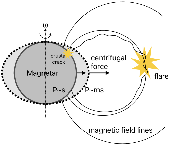
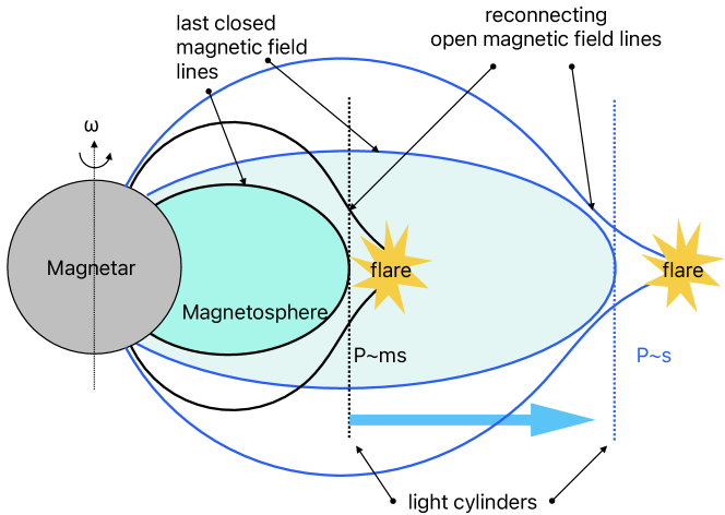
In the “star quake” paradigm, where gamma-ray flares are triggered by crustal defective events, when the magnetar is fast spinning down due to the gigantic magnetic breaking torque, the centrifugal force decreases rapidly; see Figure 1 (a). The crust of the NS will re-adjust to its new equilibrium configuration, where the centrifugal force is counteracting against the self-gravity. In this re-configuring process, crustal defective events can be expect to be much frequent than when the NS enters the later slowly spinning-down stage (such spin-down induced star quake was first discuss by Baym & Pines 1971); in the second paradigm, where gamma-ray flares are attributed to the instabilities in the magnetosphere, the boundary of the magnetar’s magnetosphere (near the light cylinder, whose radius , where is the velocity of light, and is the spin period) expand fast as its spin period rapidly increase; see Figure 1 (b). The magnetic field lines near the boundary will have to re-adjust accordingly, and thus are expected to be more likely to give-off gamma-ray flares222unlike in those conventional “solar flare” paradigm, where the magnetic twist leaks from the NS interior into the magnetosphere, through the slow crustal deformation, here the magnetic twist fast expands along with the magnetosphere. Therefore we refer to it as the “magnetosphere instability” paradigm for distinction. In fact, from our following semi-quantitative estimation we show that, the rate of gamma-ray flares in the fast spinning-down millisecond period phase is much higher than its second period phase, so that the total flare energy released in the former phase (with the time scale of days) is comparable or higher than the latter phase (with the time scale of 105 years).
In the crust crack scenarios, let us assume that each crustal destructive event which is energetic enough to trigger a magnetar gamma-ray flare has a characteristic energy . Denote the change in the centrifugal force as in a small interval of time . The corresponding linear deformation of the NS is , which we suppose is proportional to as
where is the elastic factor of the crust. The work done by the gravity is thus:
| (1) |
where denote the gravitational force acting on the crust, which remains almost constant as the deformation is small. If we equalize the work done by gravity with that released in crust cracks, we have the following equation:
| (2) |
where is the number of crust cracks in , where their ratio is the magnetar gamma-ray flare rate
which, according to equation (2), has the following proportional relationship:
| (3) |
Note that if the spinning-down torque is dominated by magnetic dipole braking333GW braking will only dominate over the magnetic braking when the spin period is less than 0.1 s (Usov, 1992; Blackman & Yi, 1998). In this case, GW braking will fast spin-down the magnetar to a regime where the magnetic braking takes over (Zhang & Mészáros, 2001)., then we have:
| (4) |
where the surface magnetic field strength, we assume to be an constant. As a result, equation (3) becomes:
| (5) |
Now, since in the first phase, the spin period is in the order of ms, and in the second phase it is s, the in the first phase can be eight orders of magnitude larger than that in the second phase. On the other hand, the time-span of the first phase is about of that of the second phase. Therefore, the magnetar gamma-ray flare energy releasing in the first phase is the same or one order of magnitude larger than that in the second phase, as we claimed in above.
If we are in the magnetosphere instability scenarios, in a short time interval , the boundary of the magnetosphere (where close and open magnetic field lines transit) expand in distance: . The volume which has been swept is:
| (6) |
The volume times the magnetic field energy density is the energy got involved. This energy is likely to be released by processes such as magnetic field re-connection near the light cylinder. We have:
| (7) |
where is the magnetic field strength at the light cylinder. For a dipole magnetic field,
Consequently, equation (7) can be reformed into:
| (8) |
Therefore, the number of bursts with characteristic energy within , i.e., the characteristic burst rate is:
| (9) |
Using the similar argument as in the crust crack scenarios, we can see the ratio of the between the first and second phase can be ten orders of magnitude, and thus the ratio of the corresponding total energy releasing can be in the magnetosphere instability scenarios.
3 The rate of flares from the population of merged magnetars
Define the magnetar flare energy differential number density distribution from a single merged-magnetar as: , where is the energy release during the flare. The total number of flares above some certain energy limit () during the life time of the magnetar is:
| (10) |
and the total energy released is:
| (11) |
which should be less than the total energy stored in the magnetosphere.
Now the rate of bursts from all merged-magnetars in the local Universe within a sphere shell of radius from to , in the energy range from to is:
| (12) |
where is the merger rate density of double neutron stars whose remnants are NSs instead of prompt collapsed BHs. The above equation can be further formulated to:
| (13) |
where is the fluence. Since , we have from the above equation that:
| (14) |
As a result, the rate of such bursts with in a limiting distance and above a limiting fluence is:
| (15) |
where is the fluence limit of the gamma-ray detector.
The volumetric integral in equation (12) should be limited to in local Universe, where the merger rate density can be viewed as a constant, and cosmic expansion has a negligible effect. When considering the joint observation of such flares with GW detection of the BNS mergers, the integral over the luminosity distance in equation (13) should be truncated at the BNS horizon of the GW detector.
The key quantities are and , where we reformulate the latter:
, where is the merger rate density of all BNS population, and is the fraction of those have long-lived magnetar remnants. can be constrained by previous GW observation at Gpc-3s-1 (The LIGO Scientific Collaboration et al., 2021).
We assume a power-law form of :
| (16) |
Studies (Cheng et al., 2020) found the index in broad consistency with that expected from a Self-Organized Criticality (SOC, see e.g., Bak et al. 1987; Lu & Hamilton 1991; Olami et al. 1992; Aschwanden 2011) process (), and the factor
Now the equation (15) can be simplified to:
| (17) |
The total energy to be released should be limited by the magnetic energy stored in the magnetosphere:
| (18) |
| (19) |
the approximant in the above equation is valid only when . Cheng et al. (2020) found , which meets the above mentioned conditions. If we assume that the flares in ordinary SGR and GFs follows the same energy distribution law, the energy of those flares can range more than five orders of magnitudes, with the corresponding to the most energetic giant flare being ergs. Therefore, from equation (19) we find that: , where is the lower energy end of the in unit of ergs.
The magnetic energy stored in the magnetosphere is (Zhang et al., 2022):
| (20) |
where is the surface magnetic field strength of the magnetar scaled with G. If we equalize the both sides of inequality (18), we can have a rough estimation of as:
| (21) |
Taking the from above, and taking ergs, with the expression of into equation (17), we have:
| (22) |
If we insert the numbers into the above equation with , we obtain that:
| (23) |
where is in unit of yr-1/Gpc3, is the distance limit in unit of 100 Mpc, is the fluence limit in unit of ergs/cm2. The detection horizon is limited by the fluence cut of a gamma-ray detector as:
| (24) |
when taking the ergs, which corresponds to a conservative estimation of the total magnetic energy stored in the magnetosphere (Zhang et al., 2022). It should be noted that, since we equalized inequality 18, the estimated occurrence rate is an upper limit.
4 Merged-magnetar flares as EM counterpart of GW events and its spin period modulation
A magnetar which was born with a millisecond spin period will experience two evolutionary phases. In its first phase of millisecond period of spinning, the magnetar’s spin period rapidly slows down to seconds by the strong magnetic braking torque. In the later phase, the spin period is settled to seconds scale and evolves less rapidly. We can define a transition time between the first and the second phases as:
| (25) |
As argued in previous sections, the burst rate before overwhelms that after it. Therefore, the rate in equation (23) mostly describes those bursts occuring before . Equivalently, those bursts to be detected is likely to following a GW chirp from BNS merger with a time lag . On the other hand, should be larger than , which is the time limit less than which, the ejecta from the BNS merger is still optically thick, thus the flares from the magnetars will be largely absorbed and the temporal structure within the flares is smeared. is also in time scale of days (Li & Paczyński 1998, and see discussion in following section).
Since the duration of a typical magnetar GF is -1 s, the flares detected in this phase can exhibit significant spin modulation, which can serve as an unambiguous evidence of the existence of a merged magnetar. In this case, the in equation (23) is the minimum between the gamma-ray detection horizon and the GW horizon:
| (26) |
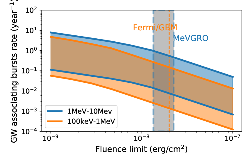
The flare rate as a function of fluence limit is plotted in Figure 2, see figure caption for the detailed description of the plot. When plotting Figure 2, we calculate the rate using equation (23) with Monte Carlo samplings of , and : is uniformly randomly sampled in log-space from 0.01 to 0.1; is sampled from a log-Gaussian distribution with 1- upper and lower limits correspond to 39 and 1900 yr-1/Gpc3; is sampled from a Gaussian random with mean 300 Mpc and a standard deviation of 40 Mpc, which corresponds to the BNS detection horizon of a GW detector network with LIGO-Virgo-KAGRA (LVK) in O4 period444as simulated here: https://emfollow.docs.ligo.org/userguide/capabilities.html.
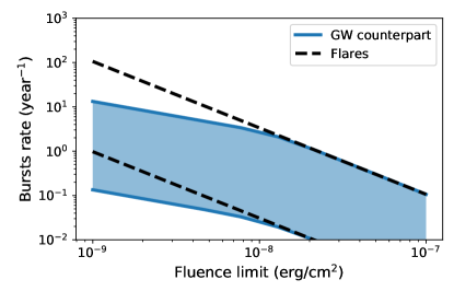
The blue band denotes the possible range of bursts rate which are associated with GW observation in LVK O4, and the dashed dark lines indicate those of bursts regardless of GW counterparts. The upper and lower limits of the range correspond to the 86% quantiles (1-sigma) in a Morte Carlo simulation.
5 Absorption by the BNS ejecta
During the collision of BNS, abundant material will be ejected from both the tidal tail and the disk (Bovard et al., 2017; Just et al., 2015). Actually BNS are the confirmed site for rapid neutron capture nucleosynthesis (-process) (Abbott et al., 2017a, b; Cowperthwaite et al., 2017; Kasen et al., 2017), which is responsible for about half of the elements heavier than iron measured in our solar system (Burbidge et al., 1957; Sneden et al., 2008). Thus, it is expected that the BNS will be surrounded by dense -process material at early time, with a total ejected mass ranging from (Bovard et al., 2017; Radice et al., 2018; Côté et al., 2018; Just et al., 2015; Fernández et al., 2015), and is optically thick to the flare gamma-ray radiation from the center remnant due to the absorption/interaction processes of photons when propagating through the material, including Compton scattering, photoelectric absorption, pair production, etc.. In the mean time, as the -process material is ejected from BNS merger with high speed, the ejecta will become optically thin at days after the merging event (Li & Paczyński, 1998; Korobkin et al., 2020; Wang et al., 2020b). The kilonova models of GW170817 observation suggested that such ejecta has a speed ranging from to on average (e.g., Kasen et al., 2017; Rosswog et al., 2018; Wollaeger et al., 2018; Watson et al., 2019), as expected from previous theoretical work (e.g., Li & Paczyński, 1998; Tanaka & Hotokezaka, 2013).
Our calculation in the previous section did not include the absorption of the surrounding BNS ejecta to the flare radiation. When such effect is included, together with a finite work energy range of the detector, it effectively replaces the limiting fluence in equations (23) and (24) with a new limiting fluence , which is related with the original as:
| (27) |
Here we define an absorption factor to describe the effect of the surrounding ejecta in absorbing the high-energy photons from the BNS flare, which is a function of time after BNS collision () and is defined as:
| (28) |
which is the ratio between the flux after absorption (observed) at time and the total emitted flux from the flare, and and denote the energy range where a specific detector works. is the differential energy flux emitted from the flare. We assume a spectrum shape of as a power law of index -0.2 with an exponentially-cutoff at MeV, i.e., , and is the normalization factor with , where is the distance of the BNS, and is the luminosity of the magnetar flare. This spectrum shape is taken from that of the GF from magnetar SGR 1806-20 (Palmer et al., 2005).
For approximation, we assume a uniform spherical -process ejecta distribution as in Wang et al. (2020a, b) to calculate the observed flare emission (after the ejecta absorption). Then, the emitted gamma rays after propagation through the ejecta (due to various photon interactions in the ejecta) is
| (29) |
where is the ejecta density, is the opacity of the ejecta to a photon with energy , path-length is the distance of the photons travelling through the ejecta, in this case, , with to be the expanding/ejected velocity of the ejecta. Only non-interacted photons are included in the observed gamma-ray signal here; scattered photons are ignored as their effects are minimal at late times when the ejecta is nearly optically thin.
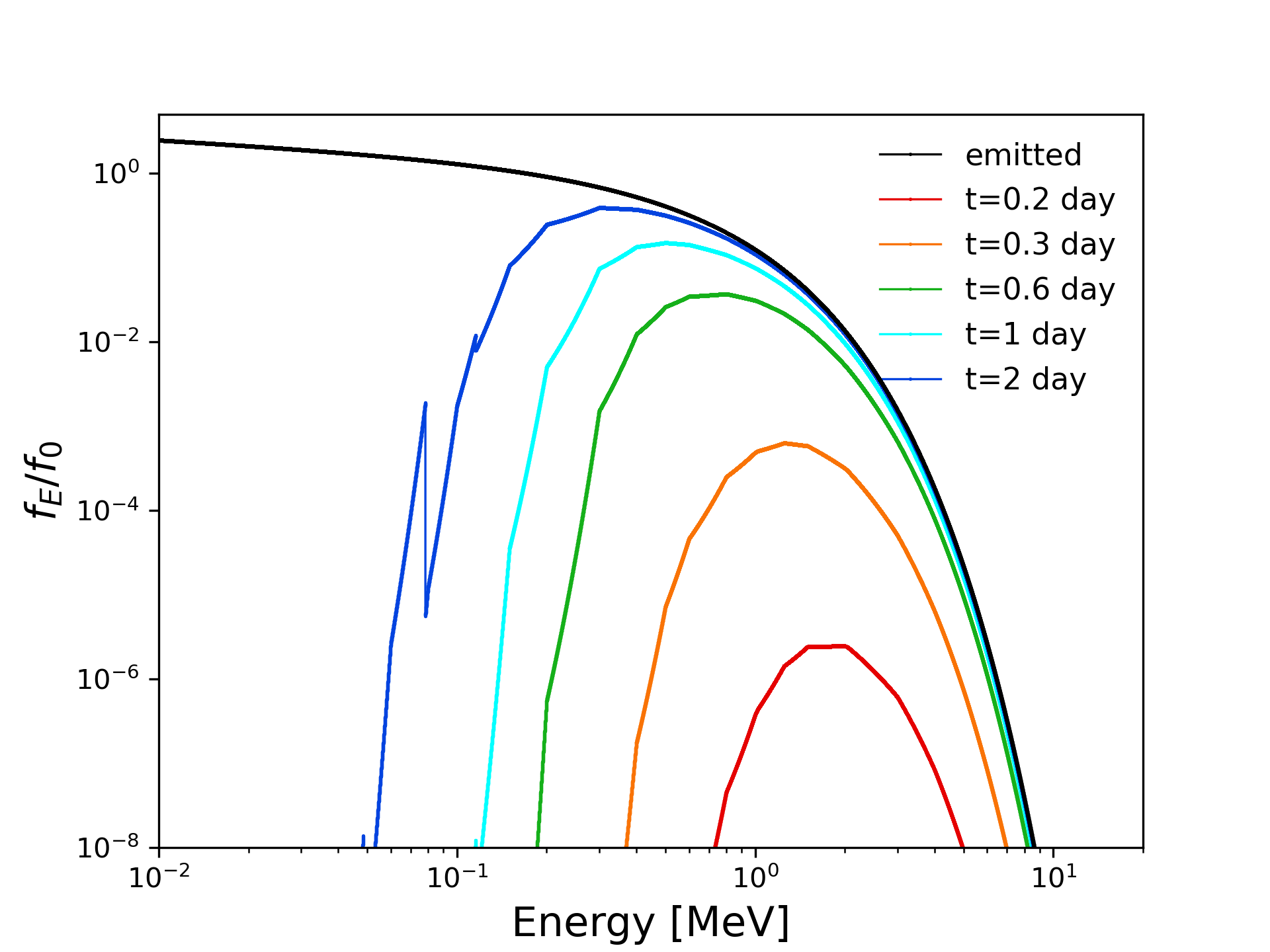
We obtain the -process nuclei abundance distribution in the BNS merger ejecta using the nuclear reaction network code Portable Routines for Integrated nucleoSynthesis Modeling, or PRISM (Mumpower et al., 2018) as in Wang et al. (2020a, b). We adopt a BNS merger dynamical ejecta with robust -process productions (Rosswog et al., 2013) for the baseline calculation. The opacity values for the total BNS collision ejecta are calculated using the ejecta’s composition with a mixture of the opacity values of five characteristic isotopes (Fe, Xe, Eu, Pt, and U), the detailed procedure is described in Wang et al. (2020b). The opacity values of individual -process nuclei are adopted from the XCOM website555https://www.nist.gov/pml/xcom-photon-cross-sections-database, with photon interactions including coherent (Rayleigh) scattering, incoherent (Compton) scattering, photoelectric absorption, and pair production. For photons with energy above MeV, the main interaction with the ejecta material is pair production; while at energy range MeV, the dominant process is incoherent (Compton) scattering; for lower energy photons (below MeV), photoelectric process mostly takes place, manifested as edges shown at energy below MeV in Figure 3, especially for the blue line that reach the energy below 0.1 MeV. Such feature arises from spikes in the BNS ejecta opacity/cross section at the same photon energies. The resulting spectra after absorption by the ejecta at 5 different times (0.2 days, 0.3 days, 0.6 days, 1 day and 2 days) after BNS collision are shown in figure 3. Compared to the emitted spectrum shown as a black line, we conclude that the detection window of such bursts should be in the energy range from 1 MeV to 10 MeV, and in the time window between 0.5 and 2 days after BNS collision.
We note that in addition to the burst flare radiation, the BNS collision ejecta itself also emit gamma-ray photons through the decays of the radioactive -process nuclei. The total gamma radiation rate from the -process ejecta is estimated to be (Metzger & Berger, 2012; Korobkin et al., 2020), and the -process gamma-ray energy at day is then erg/s for a 0.01 BNS merger ejecta. Thus, such signal would be small compared to the flare emissions, and the BNS ejecta spectrum shapes with nuclear decay lines (Korobkin et al., 2020; Wang et al., 2020b) are also different from the flare signal discussed here.
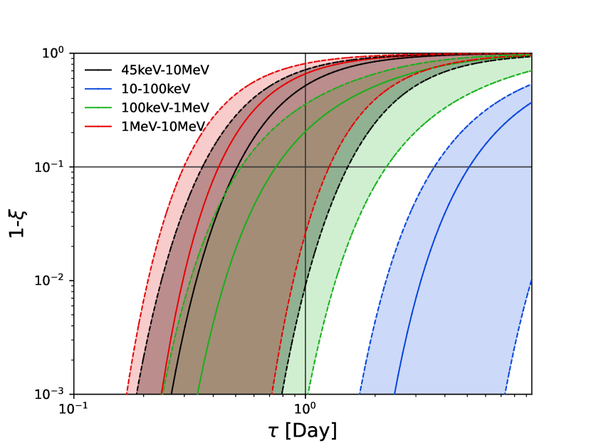
Then we conduct the integral in equation (28) to obtain as function of in Figure 4. The uncertainty bands are due to variations in BNS ejecta properties, including velocity, ejecta mass, and the components. Here we varied the ejecta mass between 0.005 to 0.03 , and the velocity between 0.1c to 0.3c. To test the sensitivity of the signal to the ejecta component, we adopted the parameterized BNS outflow conditions (Just et al., 2015; Radice et al., 2018) with a range of initial electron fractions as in Wang et al. (2020b), so that the ejecta component varies from the weak -process (no third peak and heavier actinides elements) to robust -process (with actinides). From Figure 4, we can see that at the detection window discussed above, the corresponding absorption factor is with an order of magnitude uncertainty. The burst detection rate after absorption of BNS ejecta considered is re-plotted in Figure 5. When plotting the figure, we calculate the rate with a randomly drawn from its corresponding range evaluated above with uniform distribution.
During the variation test, we find that the flare signal is more sensitive to the ejecta velocity and mass. Therefore, on the other hand, the detection rate obtained in the real observation could enable us to put a constraint on the BNS ejecta property.
6 Discussion
6.1 Potential cases in archival data from Fermi/GBM sGRB catalogue
The Fermi/GBM detector has an energy range of MeV, and a fluence limit (for a 1 s bursts) of erg/cm2 666Following the practice of Hendriks et al. (2022), we use the lowest observed fluence of the sGRB catalogue (Narayana Bhat et al., 2016) as the fluence limit of second duration bursts.. It has been monitoring GRBs for years. From our estimation, there should have been such bursts detected in its bursts catalogue. As mentioned above, such flares may exhibit spin modulation. Although there has been searches for QPOs in song of Fermi/GBM’s bright GRBs (Dichiara et al., 2013) with no positive results, a more careful survey focusing on those weak short bursts with a fast increasing period s might identify such bursts in the archival data, although with foreseeable difficulties due to their fewer photon counts. Recently, Chirenti et al. (2023) reported the detection of kHz QPOs in two archival sGRBs of the Burst and Transient Source Experiment (BATSE). BATSE works in lower energy range from 50 KeV to 300 keV, in which we expect significant absorption if they were merged-magnetar-flares. Besides, the found QPO are above 1 kHz, which is much higher than we expect for the stable merged-magnetar-flares. Therefore, these two sGRBs with QPOs should not be considered as cases of the proposed merger-magnetar-flares.
6.2 Prospects for the next generation MeV detectors
For the next generation MeV telescope, such as COSI777https://cosi.ssl.berkeley.edu, AMEGO888https://asd.gsfc.nasa.gov/amego/, or MeVGRO999https://indico.icranet.org/event/1/contributions/777/, the energy range between MeV will be well covered, and the detectors’ sensitivities at this energy range are expected to be at least 1-2 orders of magnitude better than current and previous MeV detectors like INTEGRAL101010https://www.cosmos.esa.int/web/integral and COMPTEL111111https://heasarc.gsfc.nasa.gov/docs/cgro/comptel/. However, as those detectors are not specially designed to monitor burst sources, their sensitivities to second-duration transients are much fainter than their reported value for continuous sources. Take MeVGRO as an example of the next generation MeV detectors, its fluence limit range estimated for second observing time is represented in Figure 5 as blue bands. We can tell that, using the next generation MeV detectors such as MeVGRO, the detection rate of the merged magnetar flares can only be mildly larger, or similar to that using Fermi/GBM.
The main sources of the uncertainties in the burst rate estimation is from: 1) the local rate density of the BNS collision; 2) the fraction of BNS merger which leaves long-lived magnetar, or as we denote in this paper; A future detection of a population of such bursts, together with multi-messenger observation from GW will in turn give inference on these aspects. The current BNS estimation is based on two BNS events (GW170817 and GW200311_115853) in LIGO-Virgo-Collaboration (LVC) O2-O3 period (The LIGO Scientific Collaboration et al., 2021). In the LVK-O4 period, it is estimated that BNS mergers shall be detected121212as reported in https://emfollow.docs.ligo.org/userguide/capabilities.html#datadrivenexpectations, using the same methodology in Abbott et al. (2020) but with updated input models for detector network and sources., which will return much tighter constraints on . The value of depends on the equation of state of NS matter, and also the mass function of NS. The latter can be better constraints by a larger sample of BNS observed with GWs. If multiple bursts could be observed from a single merger magnetar, the dependence of the bursts properties on its period spin could be studied, which will provide valuable insights into the emission mechanism of magnetar activities.
6.3 Solidification of the crust of the newly born magnetar
In order to justify the domination of the magnetar activity in its rapid braking stage in age of days under the star quake paradigm, we made an order-of-magnitude estimation of the burst rate in the introduction section. A crucial presumption was that the elastic property of the neutron star crust remains unchanged. First we need to check whether the surface of the NS has already cooled enough to have a solidified crust. According to Negele & Vautherin (1973); Haensel & Pichon (1994); Douchin & Haensel (2000), the melting temperature of the NS crust lies well above 108 K, and Lattimer et al. (1994) showed that the core of a newly born NS can fast cool down to temperature on the timescale:
| (30) |
Therefore, in the age of day, the new born magnetar already has a solid crust. As for its elastic properties, their are in general not constants and temperature dependent (e.g. Strohmayer et al. 1991). Therefore, a more careful quantitative calculation of the burst rate as function of the magnetar’s age should consider a realistic cooling curve of the NS’s crust and its temperature-dependent elastic properties.
6.4 Distinguishing the flaring paradigms with Galactic magnetars
The semi-quantitative argument in section 2 leads to an interesting observation: different flaring paradigm predicts a distinct flaring rate as a function of the magnetar age. More specifically, in both paradigms the characteristic flaring rate is , where for the crust crack and magnetosphere instability scenarios, respectively. Assuming that the surface magnetic field strength remains constant, and the spin down is solely contributed by magnetic dipole radiation braking, then . Therefore, the characteristic age of a magnetic is:
| (31) |
As a result,
| (32) |
One would therefore expect that by comparing the observed characteristic burst rate of the flaring activity of Galactic magnetars against prediction, it could be possible to distinct flaring paradigms.
7 Summary
From our above argument and calculation, we conclude that flares from merged massive magnetars can be expected as a population of gamma-ray transients, which associate GW chirp events of BNS mergers. Such a gamma-ray counterpart of GW may look like a short gamma-ray bursts (sGRB) according to its duration, but it can be found with several distinct features:
-
•
it tends to be weak in flux, and the time-lag between the burst and GW chirp is 1-2 days, rather than s as in sGRB;
-
•
its spectrum has a lower energy cut at 100 keV, due to absorption of the ejecta.
Besides, it may show spin modulation with a significant spin down, although the potential of significantly observing such short scale temporal structures is very challenging in reality.
Due to the absorption by the ejecta from the BNS collision, such flares are to be optimally observed in the energy range from 0.1 to 10 MeV. The estimated detection rate is increasing towards a fluence flux limit, with a power law with an index -1.5, while the rate of such bursts as GW association will also be limited by the detecting reach of GW detector networks, when the fluence limit of the HE detector is below some turn-over sensitivity. Below this turn-over fluence limit, the rate follows another power law with index -2/3. When observing with a detector of energy range 0.1-1 MeV, the turn-over flux limit is at erg/cm2, while for a detector of 1-10 MeV is at erg/cm2. Based on our evaluation from a population of BNS, a GRB monitor with energy range of MeV and a fluence limit of erg/cm2 could detect such flares as gamma-ray counterparts of GW events at a rate from 0.01 to 1 per year. To raise the detection rate of such event to a few to a few tens per year, we expect a future MeV detector working in a range from MeV with a fluence limit erg/cm2 for a 1s exposure time.
References
- Abbott et al. (2017a) Abbott, B. P., Abbott, R., Abbott, T. D., et al. 2017, Physical Review Letters, 119, 161101
- Abbott et al. (2017b) Abbott, B. P., Abbott, R., Abbott, T. D., et al. 2017, ApJ, 848, L12
- Abbott et al. (2020) Abbott, B. P., Abbott, R., Abbott, T. D., et al. 2020, Living Reviews in Relativity, 23, 3. doi:10.1007/s41114-020-00026-9
- Aschwanden (2011) Aschwanden, M. J. 2011, Self-Organized Criticality in Astrophysics, by Markus J. Aschwanden. Springer-Praxis, Berlin ISBN 978-3-642-15000-5, 416p.
- Bak et al. (1987) Bak, P., Tang, C., & Wiesenfeld, K. 1987, Phys. Rev. Lett., 59, 381. doi:10.1103/PhysRevLett.59.381
- Baym & Pines (1971) Baym, G. & Pines, D. 1971, Annals of Physics, 66, 816. doi:10.1016/0003-4916(71)90084-4
- Beloborodov (2020) Beloborodov, A. M. 2020, ApJ, 896, 142. doi:10.3847/1538-4357/ab83eb
- Blaes et al. (1989) Blaes, O., Blandford, R., Goldreich, P., et al. 1989, ApJ, 343, 839. doi:10.1086/167754
- Blackman & Yi (1998) Blackman, E. G. & Yi, I. 1998, ApJ, 498, L31. doi:10.1086/311311
- Bovard et al. (2017) Bovard, L., Martin, D., Guercilena, F., et al. 2017, Phys. Rev. D, 96, 124005
- Bransgrove et al. (2020) Bransgrove, A., Beloborodov, A. M., & Levin, Y. 2020, ApJ, 897, 173. doi:10.3847/1538-4357/ab93b7
- Burbidge et al. (1957) Burbidge, E. M., Burbidge, G. R., Fowler, W. A., & Hoyle, F. 1957, Reviews of Modern Physics, 29, 547
- Cheng et al. (2020) Cheng, Y., Zhang, G. Q., & Wang, F. Y. 2020, MNRAS, 491, 1498. doi:10.1093/mnras/stz3085
- Chirenti et al. (2023) Chirenti, C., Dichiara, S., Lien, A., et al. 2023, Nature, 613, 253. doi:10.1038/s41586-022-05497-0
- Côté et al. (2018) Côté, B., Fryer, C. L., Belczynski, K., et al. 2018, ApJ, 855, 99. doi:10.3847/1538-4357/aaad67
- Cowperthwaite et al. (2017) Cowperthwaite, P. S., Berger, E., Villar, V. A., et al. 2017, ApJ, 848, L17
- Dichiara et al. (2013) Dichiara, S., Guidorzi, C., Frontera, F., et al. 2013, ApJ, 777, 132. doi:10.1088/0004-637X/777/2/132
- Douchin & Haensel (2000) Douchin, F. & Haensel, P. 2000, Physics Letters B, 485, 107. doi:10.1016/S0370-2693(00)00672-9
- Duncan & Thompson (1992) Duncan, R. C. & Thompson, C. 1992, ApJ, 392, L9. doi:10.1086/186413
- Fahlman & Gregory (1981) Fahlman, G. G. & Gregory, P. C. 1981, Nature, 293, 202. doi:10.1038/293202a0
- Fernández et al. (2015) Fernández, R., Kasen, D., Metzger, B. D., et al. 2015, MNRAS, 446, 750. doi:10.1093/mnras/stu2112
- Ferrario & Wickramasinghe (2008) Ferrario, L. & Wickramasinghe, D. 2008, MNRAS, 389, L66. doi:10.1111/j.1745-3933.2008.00527.x
- Gavriil et al. (2002) Gavriil, F. P., Kaspi, V. M., & Woods, P. M. 2002, Nature, 419, 142. doi:10.1038/nature01011
- Golenetskii et al. (1984) Golenetskii, S. V., Ilinskii, V. N., & Mazets, E. P. 1984, Nature, 307, 41. doi:10.1038/307041a0
- Haensel & Pichon (1994) Haensel, P. & Pichon, B. 1994, A&A, 283, 313. doi:10.48550/arXiv.nucl-th/9310003
- Hartmann (1995) Hartmann, D. H. 1995, A&A Rev., 6, 225. doi:10.1007/BF01837116
- Hendriks et al. (2022) Hendriks, K., Yi, S.-X., & Nelemans, G. 2022, arXiv:2208.14156. doi:10.48550/arXiv.2208.14156
- Hurley et al. (2005) Hurley, K., Boggs, S. E., Smith, D. M., et al. 2005, Nature, 434, 1098. doi:10.1038/nature03519
- Just et al. (2015) Just, O., Bauswein, A., Ardevol Pulpillo, R., et al. 2015, MNRAS, 448, 541. doi:10.1093/mnras/stv009
- Kasen et al. (2017) Kasen, D., Metzger, B., Barnes, J., et al. 2017, Nature, 551, 80.
- Kaspi & Gavriil (2004) Kaspi, V. M. & Gavriil, F. P. 2004, Nuclear Physics B Proceedings Supplements, 132, 456. doi:10.1016/j.nuclphysbps.2004.04.080
- Kaspi & Beloborodov (2017) Kaspi, V. M. & Beloborodov, A. M. 2017, ARA&A, 55, 261. doi:10.1146/annurev-astro-081915-023329
- Kiuchi et al. (2014) Kiuchi, K., Kyutoku, K., Sekiguchi, Y., et al. 2014, Phys. Rev. D, 90, 041502. doi:10.1103/PhysRevD.90.041502
- Kluźniak & Ruderman (1998) Kluźniak, W. & Ruderman, M. 1998, ApJ, 505, L113. doi:10.1086/311622
- Komissarov et al. (2007) Komissarov, S. S., Barkov, M., & Lyutikov, M. 2007, MNRAS, 374, 415. doi:10.1111/j.1365-2966.2006.11152.x
- Korobkin et al. (2020) Korobkin, O., Hungerford, A. M., Fryer, C. L., et al. 2020, ApJ, 889, 168. doi:10.3847/1538-4357/ab64d8
- Lasky et al. (2011) Lasky, P. D., Zink, B., Kokkotas, K. D., et al. 2011, ApJ, 735, L20. doi:10.1088/2041-8205/735/1/L20
- Lattimer et al. (1994) Lattimer, J. M., van Riper, K. A., Prakash, M., et al. 1994, ApJ, 425, 802. doi:10.1086/174025
- Li & Paczyński (1998) Li, L.-X. & Paczyński, B. 1998, ApJ, 507, L59. doi:10.1086/311680
- Levin (2006) Levin, Y. 2006, MNRAS, 368, L35. doi:10.1111/j.1745-3933.2006.00155.x
- Lu & Hamilton (1991) Lu, E. T. & Hamilton, R. J. 1991, ApJ, 380, L89. doi:10.1086/186180
- Lyutikov (2003) Lyutikov, M. 2003, MNRAS, 346, 540. doi:10.1046/j.1365-2966.2003.07110.x
- Mahlmann et al. (2019) Mahlmann, J. F., Akgün, T., Pons, J. A., et al. 2019, MNRAS, 490, 4858. doi:10.1093/mnras/stz2729
- Mereghetti et al. (2015) Mereghetti, S., Pons, J. A., & Melatos, A. 2015, Space Sci. Rev., 191, 315. doi:10.1007/s11214-015-0146-y
- Mereghetti (2008) Mereghetti, S. 2008, A&A Rev., 15, 225. doi:10.1007/s00159-008-0011-z
- Metzger & Berger (2012) Metzger, B. D. & Berger, E. 2012, ApJ, 746, 48. doi:10.1088/0004-637X/746/1/48
- Minaev & Pozanenko (2020) Minaev, P. Y. & Pozanenko, A. S. 2020, Astronomy Letters, 46, 573. doi:10.1134/S1063773720090042
- Mumpower et al. (2018) Mumpower, M. R., Kawano, T., Sprouse, T. M., et al. 2018, ApJ, 869, 14
- Nakamura (1998) Nakamura, T. 1998, Progress of Theoretical Physics, 100, 921. doi:10.1143/PTP.100.921
- Narayana Bhat et al. (2016) Narayana Bhat, P., Meegan, C. A., von Kienlin, A., et al. 2016, ApJS, 223, 28. doi:10.3847/0067-0049/223/2/28
- Negele & Vautherin (1973) Negele, J. W. & Vautherin, D. 1973, Nucl. Phys. A, 207, 298. doi:10.1016/0375-9474(73)90349-7
- Norris et al. (1991) Norris, J. P., Hertz, P., Wood, K. S., et al. 1991, ApJ, 366, 240. doi:10.1086/169556
- Olami et al. (1992) Olami, Z., Feder, H. J. S., & Christensen, K. 1992, Phys. Rev. Lett., 68, 1244. doi:10.1103/PhysRevLett.68.1244
- Palmer et al. (2005) Palmer, D. M., Barthelmy, S., Gehrels, N., et al. 2005, Nature, 434, 1107. doi:10.1038/nature03525
- Radice et al. (2018) Radice, D., Perego, A., Hotokezaka, K., et al., 2018, ApJ, 869, 130
- Rea et al. (2010) Rea, N., Esposito, P., Turolla, R., et al. 2010, Science, 330, 944. doi:10.1126/science.1196088
- Rea & Esposito (2011) Rea, N. & Esposito, P. 2011, High-Energy Emission from Pulsars and their Systems, 21, 247. doi:10.1007/978-3-642-17251-9_21
- Ripperda et al. (2019) Ripperda, B., Porth, O., Sironi, L., et al. 2019, MNRAS, 485, 299. doi:10.1093/mnras/stz387
- Roberts et al. (2021) Roberts, O. J., Veres, P., Baring, M., et al. 2021, \aas
- Rosswog et al. (2013) Rosswog, S., Piran, T., & Nakar, E. 2013, MNRAS, 430, 2585. doi:10.1093/mnras/sts708
- Rosswog et al. (2018) Rosswog, S., Sollerman, J., Feindt, U., et al. 2018, A&A, 615, A132
- Ruderman et al. (2000) Ruderman, M. A., Tao, L., & Kluźniak, W. 2000, ApJ, 542, 243. doi:10.1086/309537
- Thompson (1994) Thompson, C. 1994, MNRAS, 270, 480. doi:10.1093/mnras/270.3.480
- Thompson & Duncan (1995) Thompson, C. & Duncan, R. C. 1995, MNRAS, 275, 255. doi:10.1093/mnras/275.2.255
- Thompson & Duncan (1996) Thompson, C. & Duncan, R. C. 1996, ApJ, 473, 322. doi:10.1086/178147
- Sharma et al. (2023) Sharma, P., Barkov, M., Lyutikov, M. 2023,arXiv: 2302.08848
- Sneden et al. (2008) Sneden, C., Cowan, J. J., & Gallino, R. 2008, ARA&A, 46, 241
- Spruit (1999) Spruit, H. C. 1999, A&A, 341, L1. doi:10.48550/arXiv.astro-ph/9811007
- Strohmayer et al. (1991) Strohmayer, T., Ogata, S., Iyetomi, H., et al. 1991, ApJ, 375, 679. doi:10.1086/170231
- Svinkin et al. (2021) Svinkin, D., Frederiks, D., Hurley, K., et al. 2021, Nature, 589, 211. doi:10.1038/s41586-020-03076-9
- Tanaka & Hotokezaka (2013) Tanaka, M., & Hotokezaka, K. 2013, ApJ, 775, 113
- The LIGO Scientific Collaboration et al. (2021) The LIGO Scientific Collaboration, the Virgo Collaboration, the KAGRA Collaboration, et al. 2021, arXiv:2111.03634. doi:10.48550/arXiv.2111.03634
- Turolla et al. (2015) Turolla, R., Zane, S., & Watts, A. L. 2015, Reports on Progress in Physics, 78, 116901. doi:10.1088/0034-4885/78/11/116901
- Turolla & Esposito (2013) Turolla, R. & Esposito, P. 2013, International Journal of Modern Physics D, 22, 1330024-163. doi:10.1142/S0218271813300243
- Usov (1992) Usov, V. V. 1992, Nature, 357, 472. doi:10.1038/357472a0
- Wang et al. (2020a) Wang, X., N3AS Collaboration, Fields, B. D., et al. 2020, ApJ, 893, 92. doi:10.3847/1538-4357/ab7ffd
- Wang et al. (2020b) Wang, X., N3AS Collaboration, Vassh, N., et al. 2020, ApJ, 903, L3. doi:10.3847/2041-8213/abbe18
- Watson et al. (2019) Watson, D., Hansen, C. J., Selsing, J., et al. 2019, Nature, 574, 497
- Wheeler et al. (2000) Wheeler, J. C., Yi, I., Höflich, P., et al. 2000, ApJ, 537, 810. doi:10.1086/309055
- Wollaeger et al. (2018) Wollaeger, R. T., Korobkin, O., Fontes, C. J., et al. 2018, MNRAS, 478, 3298
- Yi & Blackman (1998) Yi, I. & Blackman, E. G. 1998, ApJ, 494, L163. doi:10.1086/311192
- Yuan et al. (2020) Yuan, Y., Beloborodov, A. M., Chen, A. Y., et al. 2020, ApJ, 900, L21. doi:10.3847/2041-8213/abafa8
- Zhang & Mészáros (2001) Zhang, B. & Mészáros, P. 2001, ApJ, 552, L35. doi:10.1086/320255
- Zhang et al. (2020) Zhang, H.-M., Liu, R.-Y., Zhong, S.-Q., et al. 2020, ApJ, 903, L32. doi:10.3847/2041-8213/abc2c9
- Zhang et al. (2022) Zhang, Z., Yi, S.-X., Zhang, S.-N., Xiong, S.-L., and Xiao, S., 2022, ApJ, 939, L25. doi:10.3847/2041-8213/ac9b55