Fisher-KPP-type models of biological invasion: Open source computational tools, key concepts and analysis

Population biology can involve examining populations of individuals undergoing some form of migration mechanism together with a birth-death process. The combination of these two individual-level mechanisms can lead to the spatial expansion of that population in the form of moving density fronts. In certain contexts, these moving fronts are referred to as biological invasion or waves of biological colonisation. There are many biological and ecological applications in which biological invasion is important. These range from continental-scale ($25\times 10^{6}$ km²) colonisation of human populations over thousands of years [1] (Figure 1(a)); forest-scale ($10^{5}$ hectare) colonisation and growth of tropical rainforests over several decades [2] (Figure 1(b)); and tissue-scale (1-2 mm²) colonisation of populations of biological cells over two days [3, 4] (Figure 1(c)). As these three very disparate motivating examples indicate, the study of biological invasion, and hence the motivation to use mathematical models to explore and interrogate biological invasion, is particularly important in the field of ecology [5, 6, 7] and cell biology [9, 8]. In the field of cell biology, in particular, invasion fronts of motile and proliferative cells is important in tissue repair [10, 11, 12, 13, 14], embryonic development [15, 16, 17, 18] and disease progression, such as cancer [19, 20, 21, 22].

Continuum models of biological invasion are often extensions of the well-known Fisher-Kolmogorov (Fisher-KPP) model that was independently proposed by Fisher [23] as well as Kolmogorov, Petrovskii and Piskunov [24] in 1937,

$$\dfrac{\partial\bar{u}}{\partial\bar{t}}=\bar{D}\dfrac{\partial^{2}\bar{u}}{\partial\bar{x}^{2}}+\bar{\lambda}\bar{u}\left[1-\dfrac{\bar{u}}{\bar{K}}\right],$$

(1)

where $\bar{u}\geq 0$ is a dimensional density $[\textrm{individuals}/L^{2}]$, $\bar{D}>0$ is the diffusivity coefficient $[L^{2}/T]$ that is proportional to the rate at which individuals in the population undergo random, undirected migration, $\bar{\lambda}>0$ $[/T]$ is a growth rate associated with the logistic source term, and $\bar{K}$ is a carrying capacity density $[\textrm{individuals}/L^{2}]$. This simple reaction–diffusion model supposes that random movement of individuals in the population corresponds to a macroscopic linear diffusion term, and that the proliferation of individuals is described by a logistic growth term. While this model was first proposed as a theoretical modelling tool in 1937, it was not until 1990 that generalisations of this model were first used to explicitly study wound healing processes where $\bar{u}$ represents a density of epithelial cells that close a wound as a result of random migration and carrying capacity-limite logistic proliferation [10]. While the Fisher-KPP model involves a logistic source term, it is possible to work with a different sigmoid growth function, such as the Richards’, Gompertz or generalised logistic models [25, 26, 27].

An important feature of the Fisher-KPP model, and generalisations thereof, is the ability of these time-dependent partial differential equation (PDE) models to support travelling wave solutions. Travelling wave solutions are the long-time limit of a time-dependent solution, $\bar{t}\to\infty$ [28], where the time-dependent problem is posed on an infinite (or semi-infinite) domain with appropriate boundary conditions. The analysis of travelling wave solutions is a key topic within the applied mathematics literature [29, 30, 31, 32, 33, 34, 35, 36]. Within this context, the Fisher-KPP model is often viewed as a prototype model of high interest, especially in terms of senior undergraduate and graduate-level training in mathematical sciences [7, 9, 8]. While many methods of analysis have been deployed to interrogate and understand travelling wave solutions of the Fisher-KPP model, computational methods for solving the underlying time-dependent PDE model remain of central importance because travelling wave solutions arise as a long-time limit of the time-dependent solution of the nonlinear PDE model.

One well-known feature of travelling wave solutions of the Fisher-KPP model is that the travelling wave solutions are smooth, and do not have compact support as illustrated by the schematic travelling wave profile in Figure 1(d). This feature is at odds with many biological observations that involve a clear front position [37, 38]. This limitation of the Fisher-KPP model has been dealt with in two different ways. The first approach for introducing a sharp-fronted travelling wave solution is to generalise the linear diffusion term to a degenerate porous-media type nonlinear diffusivity [39, 40, 41, 42], giving rise to the Porous-Fisher model [9, 14, 39, 40, 41, 42, 43, 44, 45, 46, 47, 48, 49]. A second way of introducing a sharp-fronted travelling wave solution is to re-formulate the Fisher-KPP model, with linear diffusion and logistic growth, as a moving boundary model on $0<\bar{x}<\bar{L}(\bar{t})$ together with a Stefan-type boundary condition at $\bar{x}=\bar{L}(\bar{t})$ [50, 51]. This second type of generalisation has been referred to as the Fisher-Stefan model of biological invasion [52, 53, 54, 55, 56, 57, 58]. As we will show, these three relatively simple scalar reaction-diffusion models give rise to a range of interesting and partly tractable travelling wave solutions that include smooth and sharp-fronted travelling waves as illustrated in Figure 1(d)-(e). Furthermore, these models can be used to draw a distinction between invading travelling waves where $u(X,t)$ is an increasing function of time at a fixed location $X$, as well as receding travelling waves where $u(X,t)$ is a decreasing function of time at a fixed location $X$.

The aims of this review are broadly two-fold. First, we aim to provide an introduction to the well-known Fisher-KPP (Section 2) model together with details of the two lesser-known alternatives mentioned above, namely the Porous-Fisher (Section 3) and Fisher-Stefan (Section 5) models. As mentioned already, a recurring theme in our discussion will be ability of each model to describe sharp or smooth moving fronts. While all of these issues have been addressed in the literature, a feature of this review is that we will compare and contrast these three models in a single document that is accessible to graduate students and more experienced researchers alike. Second we present a series of intuitive and easy-to-use open access computational tools to generate time-dependent PDE solutions for the Fisher-KPP, Porous-Fisher and Fisher-Stefan models. Using computational tools we relate long-time PDE solutions with associated phase plane analysis and provide open access computational tools to visualise and explore the associated phase planes for travelling wave solutions of each model. We review and derive a range of various perturbation solutions that provide insight into important features of the travelling wave solutions in various asymptotic limits. Finally, we also provide, in the Appendix, another set of results for a fourth model that poses the Porous-Fisher model as a moving boundary problem which we call the Porous-Fisher-Stefan model [59, 60, 61]. Again, by providing all of our code written in the open source Julia programming language on GitHub, we aim to provide all researchers a suite of clear and practical tools to study PDE models for biological invasion that may be used directly or adapted as required.

Starting with the dimensional Fisher-KPP model, Equation (1), we re–scale density $u=\bar{u}/\bar{K}$, time $t=\bar{\lambda}\bar{t}$ and space $x=\bar{x}\sqrt{\bar{\lambda}/\bar{D}}$ to give a non-dimensional PDE model,

$$\dfrac{\partial u}{\partial t}=\dfrac{\partial^{2}u}{\partial x^{2}}+u(1-u),\quad\textrm{on}\quad 0<x<\infty,$$

(2)

whose solution $u(x,t)$ can be re-scaled to correspond to particular choices of dimensional parameters $\bar{D}$, $\bar{\lambda}$ and $\bar{K}$ for a particular application.

Relevant boundary conditions are $\partial u/\partial x=0$ at $x=0$ and $u\to 0$ as $x\to\infty$. For convenience, all time-dependent PDE problems on $0<x<\infty$ considered in this review focus on initial distributions of $u$ that are concentrated near the origin. To generate numerical solutions of Equation (2) we work on a truncated domain, $0<x<L$, where $L$ is chosen to be sufficiently large that we see clear numerical evidence of travelling wave solutions within a sufficiently long, but necessarily finite duration of time. For this study, we consider the initial condition

$$u(x,0)=\begin{cases}u_{0}&\text{if }x<b,\\ u_{0}\,\textrm{e}^{-a(x-b)}&\text{if }x>b,\end{cases}$$

(3)

where $a>0$ is the exponential decay rate of the initial density, $u_{0}>0$ is the initial maximum population density, and $b>0$ is an initial domain length where $u(x,0)=u_{0}$. For computational purposes we specify no flux boundary conditions at $x=L$, noting that if $L$ is chosen to be sufficiently large the boundary condition at $x=L$ does not play an important role in the time-dependent solution.

To explore the time-dependent solution of Equation (2) we discretize $0<x<L$ uniformly with mesh spacing $\delta x$ so that the location of the $i$th mesh point is given by $x_{i}=(i-1)\delta x$ for $i=1,2,3,\ldots,N$. For simplicity, we will write $u(x_{i},t)$ as $u_{i}$ to represent the density at the $i$th mesh point at time $t$. Taking a method-of-lines approach [62, 63], we approximate the spatial derivative terms in Equation (2) using a central difference approximation to give a system of semi-discrete coupled nonlinear ordinary differential equations (ODE),

$$\dfrac{\textrm{d}u_{i}}{\textrm{d}t}=\begin{cases}\dfrac{u_{i+1}-u_{i}}{(\delta x)^{2}}+u_{i}(1-u_{i}),&\text{if }i=1,\\ \dfrac{u_{i-1}-2u_{i}+u_{i+1}}{(\delta x)^{2}}+u_{i}(1-u_{i}),&\text{if }2\leq i\leq N-1,\\ \dfrac{u_{i-1}-u_{i}}{(\delta x)^{2}}+u_{i}(1-u_{i}),&\text{if }i=N.\end{cases}$$

(4)

Evaluating (3) on the finite difference mesh gives the initial condition for the solution of the semi-discrete system (4). This system of $N$ ODEs can be efficiently integrated through time to give $u_{i}$ for $i=1,2,3,\ldots,N$ using the DifferentialEquations.jl package in Julia [64]. Using standard convergence tolerance options, this package implements a range of numerical methods to incorporate automatic time stepping and truncation error control; for this work we implement a standard 4–5 Runge-Kutta approximation [65].

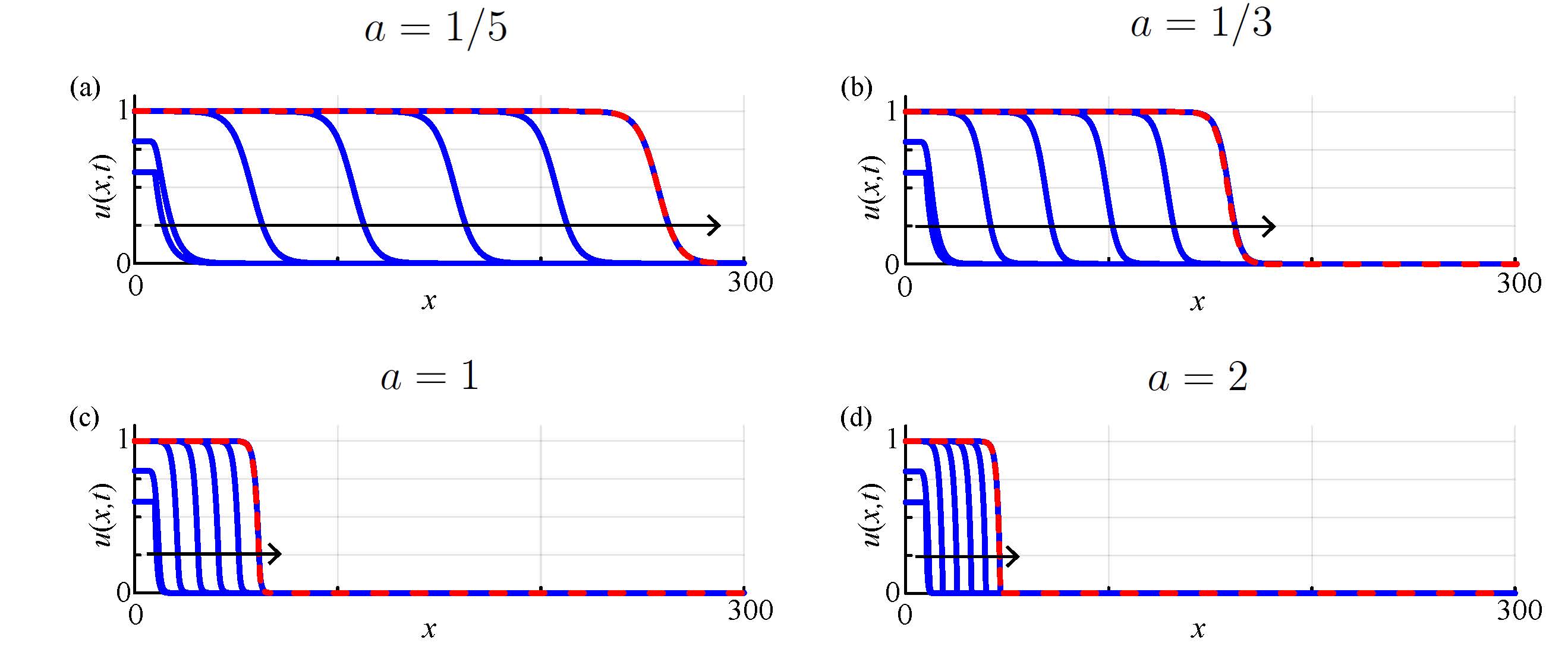
Before presenting time-dependent solutions of the Fisher-KPP model, it is worth noting that the only parameters we specify are the initial decay rate $a$, the initial length of the domain occupied by the density profile $b$, and the initial maximum density $u_{0}$. Preliminary numerical results (not shown) support the well-known results that the long-time travelling wave solutions are independent of $u_{0}$ and $b$, so we focus on the impact of different choices of $a$ for a fixed choice of $b$ and $u_{0}$. Results in Figure 2 show four different time-dependent solutions with different values of $a$; we will explain how we chose these particular values later. Results in the upper panel of Figure 2(a) correspond to $a=(5-\sqrt{21})/2$ where we show $u(x,t)$ at $t=0,1,10,20,30,40,50$ with the arrow showing the direction of increasing time. The initial condition shows the initial decay of $u(x,0)$ with position and the short-time solution $u(x,1)$ shows the impact of the logistic growth term as the density near the origin increases. The subsequent time-dependent solutions at $t=10,20,30,40,50$ illustrates that the time-dependent solution approaches a constant shape wave that appears to move with constant speed. To quantify the speed of the wave, we store the solution $u(x,t)$ at $t=0,1,2,\ldots,50$, and at each of the 51 time points we use linear interpolation to compute the value of $X$ so that $u(X,t)=1/2$. This computational procedure implicitly defines a function, $X(t)$, describing the time evolution of the position of the wave front. The lower panel of each subfigure in Figure 2 gives a scatter plot of $X(t)$ for $t=0,1,2,3,\ldots,50$ where we see that these points settle to a straight line with positive slope that represents the speed of the wave front during the simulation period. We quantify the speed of the front by taking late-time data, here chosen to be the last five time points (i.e. $t=46,47,48,49,50$) and fitting a straight line to this data to give an estimate of the speed of the front, $c$.

As suggested by the computational results in Figure 2, the long-time travelling wave speed is related to the spatial decay rate of the initial condition, $a$. It is possible to formalise this putative relationship by supposing we have $u(x,0)\sim u_{0}\textrm{exp}(-ax)$ as $x\to\infty$, and considering the motion of the leading edge where $u\ll 1$. Under these conditions the evolution of the leading edge can be approximated by the solution of a linear PDE [5] by writing $u\sim\hat{u}$, so that

$$\dfrac{\partial\hat{u}}{\partial t}=\dfrac{\partial^{2}\hat{u}}{\partial x^{2}}+\hat{u},\quad\textrm{for}\quad\hat{u}\ll 1.$$

(5)

Assuming the long-time solution takes the form of a constant speed travelling wave with an exponentially decaying front, $\hat{u}(x,t)=\textrm{const}\textrm{exp}(-a(x-ct))$, where $c$ is the travelling wave speed, we substitute this solution into the linearised PDE to give

$$c=a+\dfrac{1}{a},$$

(6)

which relates the decay rate of the initial condition $a$ to the long-time travelling wave speed, $c$. This expression is consistent with the results in Figure 2(a)–(c), however the computational results in Figure 2(d) lead to a slower observed travelling wave speed that indicated by Equation (6). The reason for the slow than expected travelling wave in Figure 2(d) is that for $a>1$, a comparison principle limits travelling wave speeds to be $c\leq 2$ [66]. Furthermore, a travelling wave analysis (below) shows that the minimum travelling wave speed possible is $c=2$, Therefore, for $a>1$ we have $c=2$. Together, these conditions give a continuous piecewise relationship

$$c=\begin{cases}a+\dfrac{1}{a},&\text{if }a<1,\\ 2,&\text{if }a>1,\end{cases}$$

(7)

where for $a$ sufficiently large the long-time travelling wave speed is independent of the initial decay rate. This explains the results in Figure 2 where we see that slowly decaying initial conditions lead to travelling wave solutions with $c>2$, whereas rapidly decaying initial conditions with $a\geq 1$ lead to travelling wave solutions that eventually move with the same minimum wave speed $c=2$. Equation (7) is often called the dispersion relationship.

To provide more insight into travelling wave solutions of the Fisher-KPP model, we explore the phase plane by writing the long time travelling wave solution as $u(x,t)=U(z)$, where $z=x-ct$. It is important to emphasise that working in the travelling wave coordinate implicitly assumes that we are dealing with a long-time solution of the time-dependent PDE where a constant speed and constant shape travelling wave solution has developed. Under these conditions, transforming the time-dependent PDE model into the travelling wave coordinate gives

$$\dfrac{\textrm{d}^{2}U}{\textrm{d}z^{2}}+c\dfrac{\textrm{d}U}{\textrm{d}z}+U(1-U)=0,\quad\textrm{on}\quad-\infty<z<\infty,$$

(8)

with boundary conditions

$$\lim_{z\to\infty}U(z)=0,\quad\textrm{and}\quad\lim_{z\to-\infty}U(z)=1.$$

(9)

Note that (8)–(9) is invariant under translation in $z$, which means that we may fix the solution by setting $U(0)=1/2$, for example. Exact, closed-form solutions of this boundary value problem for $U(z)$ are unknown except for the special case of $c^{2}=25/6$ where (8) has the Painlevé property [30, 36].

To make progress, we study the solution of (8)–(9) in the $(U,V)$ phase plane, where

	$\displaystyle\dfrac{\textrm{d}U}{\textrm{d}z}$	$\displaystyle=V,$		(10)
	$\displaystyle\dfrac{\textrm{d}V}{\textrm{d}z}$	$\displaystyle=-cV-U(1-U).$		(11)

At this point it is interesting to comment on the differences between studying travelling wave solutions of the Fisher-KPP model using the phase plane as opposed to considering long-time solutions of the time-dependent PDE model. As we pointed out previously, the latter involves specifying details of the initial condition, such as the decay rate $a$, and then solving the PDE to estimate the long-time travelling wave speed $c$ as an output of this computational task. In contrast, working with the phase plane implicitly assumes that we have moved to the long–time limit where a travelling wave solution $U(z)$ is relevant, which involves specifying the travelling wave speed $c$ as an input to this separate computational task. This means that we can visualise the phase plane for any value of $c$ that we choose, regardless of whether that value arises as a long–time output of a time–dependent PDE solution. This includes travelling wave solutions that are physically unrealistic, as we will explain and demonstrate later.

The dynamical system governing the phase plane (10)–(11) has two equilibrium points: $(\bar{U},\bar{V})=(0,0)$ and $(\bar{U},\bar{V})=(1,0)$. Linear stability indicates that $(\bar{U},\bar{V})=(1,0)$ is a saddle point for all values of $c$. The unstable and stable manifolds near the saddle point tend to straight lines passing through $(\bar{U},\bar{V})=(1,0)$ with slopes given by

$$m_{\pm}=\dfrac{-c\pm\sqrt{c^{2}+4}}{2}.$$

(12)

Linear stability analysis indicates that $(\bar{U},\bar{V})=(0,0)$ is a stable spiral for $c<2$ and a stable node for $c\geq 2$. As we shall explain, this bifurcation at $c=2$ shows that all physically realistic travelling wave solution to the Fisher-KPP model have $c\geq 2$.

With this information, we can now visualise various phase planes and explore the consequences of varying $c$. Results in Figure 3 illustrate key features of the phase planes for $c=3,2,1$, respectively. Trajectories in the phase planes are obtained by solving (10)–(11) numerically using DifferentialEquations.jl in Julia. The phase plane in Figure 3(a) for $c=3$ shows the two equilibria and a range of trajectories in blue that are included to provide visual interpretation of the full dynamical system. Each blue trajectory is a valid solution of (10)–(11), but these solutions are not relevant in the sense that they are not related to travelling wave solutions of the Fisher-KPP model since they do not satisfy the boundary conditions (9). We also show three yellow trajectories and one red trajectory. These four trajectories enter and leave the equilibrium point at $(1,0)$ along the stable and unstable manifolds and plotting these four trajectories on the phase plane makes the point that $(1,0)$ is a saddle point. The red trajectory that leaves $(1,0)$ along the unstable manifold into the fourth quadrant of the $(U,V)$ phase plane enters the origin to form a heteroclinic orbit. Of all the trajectories plotted in the phase plane, it is only this red heteroclinic orbit that has a physical interpretation in terms of the travelling wave solution since it satisfies the boundary conditions (9).

We can interpret this red heteroclinic orbit in the phase plane as a parametric curve $(U(z),V(z))$ from which we can plot $U(z)$ and compare the shape of this curve, after applying an appropriate shift in $z$, with a long-time solution of the time-dependent PDE. The dashed red curve in Figure 2(b) corresponds to $U(z)$ generated in the phase plane, appropriately shifted and superimposed on the late-time PDE solution $u(x,50)$. Comparing these two curves shows that the shape of the travelling wave solution obtained from the phase plane is visually indistinguishable from the shape of the late-time PDE solution on this scale. Indeed, each upper panel in the four subplots in Figure 2 compares the shape of a late-time PDE solution with the shape of $U(z)$, appropriately shifted, obtained from the phase plane for the corresponding value of $c$.

Results in Figure 3(b) shows a similar phase plane, together with many illustrative blue solution trajectories and the three yellow and one red solution trajectory for $c=2$. Linear stability indicates that the solution of (10)–(11) locally near the origin bifurcates at $c=2$ since the origin is a stable node for $c\geq 2$ and a stable spiral for $c<2$. The borderline case of $c=2$, shown in Figure 3(b) indicates that the heteroclinic orbit enters the origin with $U>0$ as $z\to\infty$. Taking the shape of the $U(z)$ solution from the phase plane, shifting this profile and superimposing on the late-time PDE solutions in Figure 2(c)–(d) shows that the shape of the wave obtained from the phase plane is visually indistinguishable from these two late-time PDE solutions that evolved from different initial conditions.

The phase plane in Figure 2(c) for $c=1$ shows similar features to the two previous phase planes with the exception that we now see the solution of (10)–(11) spirals into the origin, which implies that $U<0$ over infinitely many subintervals for $z>0$. While this trajectory is a valid solution of the dynamical system together with the boundary conditions (9), the heteroclinic orbit is not physical in the sense that it does not relate to a late-time solution of the Fisher-KPP model. Therefore, we see that from phase-plane analysis alone, we must have $c\geq 2$. Furthermore, this example makes the point we alluded to earlier that working in the phase plane allows us to specify a value of $c$ regardless of whether that value relates to a long-time output of a time-dependent PDE solution. This observation has often led researchers to discard this phase plane for $c<2$, however we will revisit this question later in Section 5 when we consider the Fisher-Stefan model.

Computational explorations of the time-dependent solutions of the Fisher-KPP model, along with our leading edge and phase plane analysis confirm that travelling wave solutions of the Fisher-KPP model involve $c\geq 2$. We will now show that it is possible to develop some mathematical insight into the shape of these travelling waves in the limit $c\to\infty$ by following Canosa [28]. Introducing the change of coordinates $\xi=z/c$ allows us to re-write Equation (8) as

$$\dfrac{1}{c^{2}}\dfrac{\textrm{d}^{2}U}{\textrm{d}\xi^{2}}+\dfrac{\textrm{d}U}{\textrm{d}\xi}+U(1-U)=0,\quad\textrm{on}\quad-\infty<z<\infty,$$

(13)

with boundary conditions

$$\lim_{\xi\to\infty}U(\xi)=0,\quad\textrm{and}\quad\lim_{\xi\to-\infty}U(\xi)=1.$$

(14)

Identifying the small parameter $c^{-1}$ and assuming the solution can be written as a regular perturbation expansion [67]

$$U(\xi)=U_{0}(\xi)+\left(\dfrac{1}{c^{2}}\right)U_{1}(\xi)+\mathcal{O}\left(\dfrac{1}{c^{4}}\right),$$

(15)

we substitute this expansion into (13) to give

	$\displaystyle\dfrac{\textrm{d}U_{0}}{\textrm{d}\xi}$	$\displaystyle=-U_{0}(1-U_{0}),\quad U_{0}(0)=\dfrac{1}{2},$		(16)
	$\displaystyle\dfrac{\textrm{d}U_{1}}{\textrm{d}\xi}$	$\displaystyle=-\dfrac{\textrm{d}^{2}U_{0}}{\textrm{d}\xi^{2}}-U_{1}(1-2U_{0}),\quad U_{1}(0)=0,$		(17)

whose solutions, $U_{0}(\xi)$ and $U_{1}(\xi)$, can be written in terms of the original independent variable as

	$\displaystyle U_{0}(z)$	$\displaystyle=\dfrac{1}{1+\textrm{e}^{z/c}},$		(18)
	$\displaystyle U_{1}(z)$	$\displaystyle=\dfrac{\textrm{e}^{z/c}}{\left(1+\textrm{e}^{z/c}\right)^{2}}\ln\left[\dfrac{4\textrm{e}^{z/c}}{\left(1+\textrm{e}^{z/c}\right)^{2}}\right].$		(19)

With these expressions for $U_{0}(z)$ and $U_{1}(z)$, we now have a two-term perturbation solution $U(z)=U_{0}(z)+c^{-2}U_{1}(z)$ that provides insight into how the shape of the travelling wave solution relates to the travelling wave speed $c$. Profiles in Figure 4(a) compare the leading order solution $U_{0}(z)$, and the two-term perturbation solution $U_{0}(z)+c^{-2}U_{1}(z)$ with a late-time solution of the time-dependent PDE for $c=3$. In this case we see that the leading order solution provides a very good approximation of the full travelling wave solution since the differences between the numerical result and the perturbation solution barely evident at this scale. Further, we see that the two-term perturbation solution is visually indistinguishable from the numerical solution at this scale. Profiles in Figure 4(b) are for the minimum travelling wave speed, $c=2$, where again we see that the two-term perturbation solution accurately matches the numerical result. The fact that the perturbation solution performs very well for the minimum travelling wave speed illustrates how useful perturbation solutions can be as we are unable to obtain closed form exact solutions for arbitrary values of $c$, yet these approximate solutions valid in the limit that $c\to\infty$ turn out to be relatively accurate for just $c=2$.

More generally, our perturbation solution provides insight into the relationship between the shape of the travelling wave solution and the speed of the wave, $c$. For example, evaluating the $\mathcal{O}(1)$ perturbation solution at $z=0$ gives

$$\dfrac{\textrm{d}U}{\textrm{d}z}=-\dfrac{1}{4c}+\mathcal{O}\left(\dfrac{1}{c^{2}}\right),$$

(20)

indicating that the faster the travelling wave speed, the flatter the shape of the wave since we have $\textrm{d}U/\textrm{d}z\to 0^{-}$ as $c\to\infty$ [9].

As explained in Section 2, one of the limitations of travelling wave solutions of the Fisher-KPP model is that they are smooth with $u>0$ for all $x>0$, which means that it is difficult to unambiguously identify the precise position of the leading edge of the moving front. This is a challenge because experimental observations often lead to clearly defined sharp fronts that are incompatible with this feature of the Fisher-KPP model [11, 12, 42]. As such, considerable effort has been spent in developing and understanding alternative reaction-diffusion models that lead to travelling wave solutions with compact support so that these solutions can be used to clearly identify the position of the moving front. Possibly the most common approach is to work with the Porous-Fisher model, which can be written in non-dimensional form as

$$\dfrac{\partial u}{\partial t}=\dfrac{\partial}{\partial x}\left[u\dfrac{\partial u}{\partial x}\right]+u(1-u),\quad\textrm{on}\quad 0<x<\infty,$$

(21)

with $\partial u/\partial x=0$ at $x=0$ and $u\to 0$ as $x\to\infty$. The key difference is that the linear diffusion flux in the Fisher-KPP model $\mathcal{J}=-\partial u/\partial x$ is replaced with a degenerate nonlinear diffusive flux $\mathcal{J}=-u\,\partial u/\partial x$ so that $\mathcal{J}$ vanishes when $u=0$ [39, 41, 49]. For numerical purposes, we will replace the far-field condition with $\partial u/\partial x=0$ at $x=L$, where the value of $L$ is chosen to be sufficiently large so that this does not affect our numerical solution. We will consider the same initial condition as for the Fisher-KPP model, namely (3). To explore time-dependent solutions of the Porous-Fisher model we discretise Equation (21) on the same equally-spaced finite difference mesh to give,

$$\dfrac{\textrm{d}u_{i}}{\textrm{d}t}=\begin{cases}\dfrac{(u_{i+1}+u_{i})(u_{i+1}-u_{i})}{2(\delta x)^{2}}+u_{i}(1-u_{i}),&\text{if }i=1,\\ \dfrac{(u_{i+1}+u_{i})(u_{i+1}-u_{i})-(u_{i-1}+u_{i})(u_{i}-u_{i-1})}{2(\delta x)^{2}}+u_{i}(1-u_{i}),&\text{if }2\leq i\leq N-1,\\ \dfrac{(u_{i-1}+u_{i})(u_{i-1}-u_{i})}{2(\delta x)^{2}}+u_{i}(1-u_{i}),&\text{if }i=N,\end{cases}$$

(22)

which can be integrated through time using the same Julia package as for the Fisher-KPP model. The inputs into these time-dependent PDE solutions are the parameters governing the initial condition $u_{0}$, $a$ and $b$; long-time PDE solutions can be used to estimate the travelling wave speed, $c$. Again, as for the Fisher-KPP model, preliminary explorations (now shown) indicate that $c$ depends upon $a$, but is independent of $u_{0}$ and $b$.

Results in Figure 5 illustrate time-dependent solutions of the Porous-Fisher model with the initial condition given by Equation (3) with $a=1/5,1/3,1,2$. In each case, we see the eventual formation of a constant speed, constant shape travelling wave. Using the same approach as for the Fisher-KPP model, we trace the evolution of $X(t)$, where $u(X,t)=0.5$, to generate a time series of $X(t)$ data which eventually falls on a straight line with a positive slope. Fitting a straight line regression model to the last five points in this time series gives us an estimate of $c$. Details of the $X(t)$ data and the straight line regression plot are not shown here as they look almost identical to those shown in Figure 2 for the Fisher-KPP model. More information can be obtained by exploring the time-dependent PDE codes available on GitHub.

An important point illustrated by the time-dependent PDE solutions in Figure 5 is that solutions with sufficiently slow initial decay rates lead to fast, smooth-fronted travelling wave solutions that qualitatively resemble travelling wave solutions to the Fisher-KPP model in Figure 2. Later in this Section we will provide a mathematical explanation of this observation. On the other hand, highlighted in Figure 5(d) is that the smooth initial condition with a sufficiently fast exponential decay appears to evolve into a sharp-fronted travelling wave with a well-defined front position. This is a very different outcome to the Fisher-KPP case and may be interpreted as a favourable feature in terms of mathematical modelling. We will investigate the sharp-fronted solution later when we explore these travelling wave solutions in the phase plane, and then provide a more detailed explanation of these results in Section 4.

From a numerical point of view it is worth noting that results in Figures 2 and 3 are obtained on the same domain, $0\leq x\leq 300$, but we have used a much finer discretisation to explore time-dependent solutions of the Porous-Fisher model. Our explorations (not shown) indicate that smooth-fronted solutions of the Porous-Fisher model and the Fisher-KPP model can be obtained using a relatively coarse discretisation (e.g. $\delta x=0.1$) leading to grid-independent results when plotted on this scale. The situation is different, however, with the apparent sharp-fronted solution of the Porous-Fisher model in Figure 3(d) where we require a much finer numerical discretisation to accurately resolve the shape of the leading edge of the travelling wave, and to provide an accurate estimate of $c$. Therefore, unlike the Fisher-KPP model where we find that it is possible to make an appropriate choice of $\delta x$ so that the numerical algorithm performs reasonably well for a range of $a$ values, much greater care needs to be exercised when solving the Porous-Fisher model numerically because the possibility of sharp-fronted solutions requires much finer resolution. For simplicity, all results in Figure 5 are generated with a much finer mesh resolution than the results in Figure 2 for the Fisher-KPP model. We encourage the reader to explore the impact of choosing different values of $\delta x$ using the code provided as it is straightforward to show that smooth travelling wave solutions of the Porous-Fisher model can be very accurate with a much coarser mesh.

Just as we did for the smooth-fronted travelling wave solutions of the Fisher-KPP model, it is possible to relate the long-time travelling wave speed $c$ to the decay rate of the initial condition for smooth-fronted travelling wave solutions of the Porous-Fisher model. Supposing we have $u(x,0)\sim u_{0}\textrm{exp}(-ax)$ as $x\to\infty$ for $a>0$, we can examine the motion of the leading edge by writing $u\sim\hat{u}$ so that

$$\dfrac{\partial\hat{u}}{\partial t}=\hat{u},\quad\textrm{for}\quad\hat{u}\ll 1.$$

(23)

If the travelling wave solution of (21) takes the form $\hat{u}(x,t)=\textrm{const}\,\textrm{exp}(-a(x-ct))$, substituting this solution into the linearised PDE (23) gives the dispersion relationship for the Porous-Fisher model

$$c=\dfrac{1}{a},$$

(24)

which is consistent with the smooth-fronted travelling wave solutions presented in Figure 5(a)–(c).

Unlike the Fisher-KPP model, the minimum travelling wave speed for travelling wave solutions of the Porous-Fisher model cannot be determined solely by examining the dispersion relationship and we now turn to the phase plane by writing the long-time travelling wave solution as $u(x,t)=U(z)$, where $z=x-ct$. Transforming the time-dependent PDE model into the travelling-wave coordinate gives

$$\dfrac{\textrm{d}}{\textrm{d}z}\left[U\dfrac{\textrm{d}U}{\textrm{d}z}\right]+c\dfrac{\textrm{d}U}{\textrm{d}z}+U(1-U)=0,\quad\textrm{on}\quad-\infty<z<\infty,$$

(25)

with boundary conditions

$$\lim_{z\to\infty}U(z)=0,\quad\textrm{and}\quad\lim_{z\to-\infty}U(z)=1.$$

(26)

As for travelling wave solutions of the Fisher-KPP model, it is not obvious how to solve Equation (25) for arbitrary values of $c$, so we study the solution of this boundary value problem in the $(U,V)$ phase plane where we have [9]

	$\displaystyle\dfrac{\textrm{d}U}{\textrm{d}z}$	$\displaystyle=V,$		(27)
	$\displaystyle U\dfrac{\textrm{d}V}{\textrm{d}z}$	$\displaystyle=-cV-U(1-U)-V^{2}.$		(28)

This dynamical system is singular when $U=0$. The singularity can be removed by introducing a transformed independent variable that we write implicitly as [9]

$$\dfrac{\textrm{d}}{\textrm{d}\zeta}=U\dfrac{\textrm{d}}{\textrm{d}z},$$

(29)

which gives a de-singularised system

	$\displaystyle\dfrac{\textrm{d}U}{\textrm{d}\zeta}$	$\displaystyle=UV,$		(30)
	$\displaystyle\dfrac{\textrm{d}V}{\textrm{d}\zeta}$	$\displaystyle=-cV-U(1-U)-V^{2}.$		(31)

This desingularised phase plane is has three equilibria: $(\bar{U},\bar{V})=(0,0)$, $(\bar{U},\bar{V})=(1,0)$ and $(\bar{U},\bar{V})=(0,-c)$. Linear stability analysis indicates that both $(\bar{U},\bar{V})=(1,0)$ and $(\bar{U},\bar{V})=(0,-c)$ are saddle points for all values of $c$, while the origin is a stable nonlinear node. Similar to the Fisher-KPP model, smooth travelling waves are associated with a heteroclinic orbit between $(1,0)$ and $(0,0)$, but we now have the possibility of a sharp-fronted heteroclinic orbit between $(1,0)$ and $(0,-c)$. In this case the heteroclinic orbit terminates at $(U,V)=(0,-c)$ meaning that the contact point, where $U=0$, has a finite negative slope for $c>0$.

Computationally-generated phase planes with various trajectories highlighted are given in Figure 6 for key choices of $c=1,1/\sqrt{2},1/2$. The phase plane in Figure 6(a) for $c=1$ shows a range of blue trajectories obtained by solving (30)–(31) numerically using codes provided on GitHub. These blue trajectories provide a visual picture of the phase plane within the vicinity of the three equilibrium points. The phase plane also includes seven yellow trajectories that either enter or leave $(0,-c)$ and $(1,0)$ along the associated unstable and stable manifolds of these saddle node points. Finally, in red we show the heteroclinic orbit leaving $(1,0)$ along the unstable manifold into the fourth quadrant of the $(U,V)$ phase plane, eventually entering the origin. This heteroclinic orbit corresponds to the smooth travelling wave solution in Figure 5(c).

Exploring various phase planes by gradually reducing $c<1$ indicates that smooth travelling wave solutions, corresponding to a heteroclinic orbit between $(1,0)$ and $(0,0)$, persist until we reach some critical value of $c$ where, as the equilibrium point at $(0,-c)$ moves up the $V$-axis, it becomes possible to have a straight-line heteroclinic orbit between $(1,0)$ and $(0,-c)$, as illustrated in Figure 6(b). The straight-line heteroclinic orbit, $V=-c(1-U)$, can be substituted into (30)–(31) to show that the corresponding special travelling wave speed is $c=1/\sqrt{2}$ [9]. This orbit corresponds to a sharp-fronted travelling wave solution like the results we obtained numerically in Figure 5(d). Since we now have a mathematical expression for the straight line heteroclinic orbit in the phase plane, we can give a closed-form expression for this special sharp-fronted solution

$$U(z)=\begin{cases}1-\textrm{e}^{z/\sqrt{2}},&\text{if }z\leq 0,\\ 0,&\text{if }z>0,\end{cases}$$

(32)

where this solution has been arbitrarily shifted so the position of the front is $z=0$. This solution is significant because, unlike the Fisher-KPP model, the Porous-Fisher model leads to travelling wave solutions with a natural front position meaning that this feature can be used to match with experimental observations more easily than working with a smooth–fronted travelling wave solution [14, 47]. To complete the picture, Figure 6(c) shows a phase plane and associated trajectories for $c=1/2<1/\sqrt{2}$ where we now see that there is no longer any possibility of a heteroclinic orbit, indicating that $c=1/\sqrt{2}$ is the minimum travelling wave speed for the Porous-Fisher model.

For smooth-fronted travelling wave solutions with $c>1/\sqrt{2}$ we can numerically integrate (30)–(31) to give numerical estimates of the trajectory in the $(U,V)$ phase plane. This trajectory can be interpreted as a parameterised curve with parameter $\zeta$. Our numerical algorithms on GitHub solve for $U(\zeta)$ and $V(\zeta)$, recording values of these quantities at equally-spaced intervals of $\zeta$, with spacing $\delta\zeta$. To compare our numerical estimate of $U(\zeta)$ with numerical solutions of the full time-dependent PDE model in Figure 5 we use (29) to relate $\zeta$ and $z$, noting that

$$z(\zeta)=\int^{\zeta}U(\zeta^{\prime})\,\textrm{d}\zeta^{\prime},$$

(33)

can be evaluated numerically to give a relationship between $z$ and $\zeta$. Since we store values of $U(\zeta)$ at equally-spaced intervals of $\zeta$, it is straightforward to compute $z(\zeta)$ by applying the trapezoid rule to evaluate the integral in (33). While other quadrature methods could be implemented, our approach is simple to implement, and leads to estimates of $U(z)$ that, after appropriate shifting, compare well with various late-time PDE solutions. Each smooth-fronted time-dependent PDE solution in Figure 5(a)–(c) includes a dashed red line superimposed on $u(x,50)$. These dashed red lines correspond to the appropriately shifted $U(z)$ profile obtained from the phase planes; we see that the shape of the travelling wave solution from the time-dependent PDE solution is visually indistinguishable from the profile obtained using the phase plane trajectories. The result in Figure 5(d) for the sharp-fronted travelling wave moving with the minimum travelling wave speed compares the late time PDE solution with the shifted exact solution, Equation (32). Again, as for the smooth-fronted travelling wave solutions, here we see that the time-dependent PDE solutions at late time are visually indistinguishable, at least at this scale, from the exact phase plane result.

To conclude this investigation into travelling wave solutions of the Porous-Fisher model evolving from smooth initial conditions, we now develop approximate perturbation solutions to describe the shape of smooth-fronted travelling wave solutions in the limit $c\to\infty$. Introducing the change of coordinates, $\xi=z/c$, gives

$$\dfrac{1}{c^{2}}\dfrac{\textrm{d}}{\textrm{d}\xi}\left[U\dfrac{\textrm{d}U}{\textrm{d}\xi}\right]+\dfrac{\textrm{d}U}{\textrm{d}\xi}+U(1-U)=0,\quad\textrm{on}\quad-\infty<\xi<\infty,$$

(34)

with boundary conditions

$$\lim_{\xi\to\infty}U(\xi)=0,\quad\textrm{and}\quad\lim_{\xi\to-\infty}U(\xi)=1.$$

(35)

Treating $c^{-1}$ as a small parameter, we assume that the solution can be written as

$$U(\xi)=U_{0}(\xi)+\left(\dfrac{1}{c^{2}}\right)U_{1}(\xi)+\mathcal{O}\left(\dfrac{1}{c^{4}}\right).$$

(36)

Substituting this expansion into (34) gives

	$\displaystyle\dfrac{\textrm{d}U_{0}}{\textrm{d}\xi}$	$\displaystyle=-U_{0}(1-U_{0}),\quad U_{0}(0)=\dfrac{1}{2},$		(37)
	$\displaystyle\dfrac{\textrm{d}U_{1}}{\textrm{d}\xi}$	$\displaystyle=-\dfrac{\textrm{d}}{\textrm{d}\xi}\left[U_{0}\dfrac{\textrm{d}U_{0}}{\textrm{d}\xi}\right]-U_{1}(1-2U_{0}),\quad U_{1}(0)=0,$		(38)

whose solutions, $U_{0}(\xi)$ and $U_{1}(\xi)$ can be written in terms of the original independent variable as,

	$\displaystyle U_{0}(z)$	$\displaystyle=\dfrac{1}{1+\textrm{e}^{z/c}},$		(39)
	$\displaystyle U_{1}(z)$	$\displaystyle=\dfrac{\textrm{e}^{z/c}}{\left(1+\textrm{e}^{z/c}\right)^{2}}\left[\ln 2-\dfrac{3}{2}+\dfrac{3+\left(1+\textrm{e}^{z/c}\right)\left[z/c-\ln\left(1+\textrm{e}^{z/c}\right)\right]}{1+\textrm{e}^{z/c}}\right].$		(40)

These expressions give a two-term perturbation solution $U(z)=U_{0}(z)+c^{-2}U_{1}(z)$ which provides insight into how the shape of the travelling wave solution relates to $c$, as we will now explore.

Profiles in Figure 7(a) compare the leading order solution $U_{0}(z)$, and the two-term perturbation solution $U_{0}(z)+c^{-2}U_{1}(z)$ with a late-time solution of the time-dependent PDE for $c=3$. As for the Fisher-KPP model, we see that the leading order solution provides a good approximation of the numerical solution of the full problem. It is useful to recall that travelling wave solutions of the Fisher-KPP model are restricted to $c\geq 2$ and in Figure 4(b) we saw that a large $c$ asymptotic approximation performed well, even for $c=2$. With the Porous-Fisher model we have smooth travelling wave solutions for $c>1/\sqrt{2}$ which means we can explore the accuracy of a large $c$ asymptotic approximation for even smaller values of $c$ than was possible with the Fisher-KPP model. Profiles in Figure 7(b) for $c=1$ illustrate that the $U_{0}(z)$ solution is visually-distinct from the full time-dependent solution whereas the two term solution gives a reasonably accurate approximation of the shape of the wave, which is remarkable given that we have $c=1$ and the perturbation approximation is valid for $c\to\infty$.

It is insightful to note that the $U_{0}(z)$ term in the large $c$ perturbation solution is identical for the Fisher-KPP and Porous-Fisher models. There are several inferences that can be drawn from this observation. First, we have the same qualitative relationship between the shape and speed of the travelling wave, namely the faster the travelling wave the flatter the shape of the travelling wave for sufficiently large $c$ for both models. Second, this indicates that the shape of a fast-moving travelling wave is primarily determined by the source term in the PDE model rather than the flux term because the influence of the diffusive flux term arises as a correction term whereas the proliferation mechanism controls the leading order features. This is biologically insightful because while both diffusion and a source term are required to form a travelling wave solution, it is the proliferation term that largely controls the shape of the travelling wave [16].

All time-dependent PDE solutions considered in Sections 2–3 are mathematically convenient since they have $u(x,0)\sim u_{0}\,\textrm{exp}(-ax)$ as $x\to\infty$ for $a>0$. This means that the initial conditions shown in Figures 2 and 5 are smooth with $u(x,0)>0$ for all $x>0$. This form of initial condition allows us derive a dispersion relationship that relates the exponential decay rate $a$ to the long-time travelling wave speed $c$, and our time-dependent PDE solutions in Figures 2 and 5 are consistent with the dispersion relationship in both cases. This approach, however, is not always preferred since real applications of biological invasion are unlikely to involve an initial distribution that decays exponentially with position [3, 1]. An alternative approach is to consider an initial condition of the form

$$u(x,0)=\begin{cases}u_{0},&\text{if }0<x<b,\\ 0,&\text{if }x>b,\end{cases}$$

(41)

which is far more practical because it models some initial region that is occupied at density $u_{0}$, that is adjacent to another region, $x>b$, which is completely vacant with $u=0$. This is precisely the kind of initial condition that is used in the case of applications in cell biology, such as modelling scratch assay experiments [14, 16, 11, 12].

Using our time-dependent PDE algorithms we can confirm that long-time shape and speed of the Fisher-KPP and Porous-Fisher solution profiles with the initial condition (41) are independent of the choice of $u_{0}$ and $b$ (not shown). For example, typical time-dependent solutions are shown in Figure 8 where we see that the long-time travelling wave solution of the Fisher-KPP model evolves to the travelling wave solution with the minimum wave speed $c=2$, while the long time travelling wave solution of the Porous-Fisher model also evolves to the travelling wave solution with the minimum wave speed with $c=1/\sqrt{2}$.

It is useful to know that travelling wave solutions evolving from initial conditions with compact support lead to travelling wave solutions with the minimum wave speed. For the Fisher-KPP model this is consistent with the observation that (41) can be interpreted as taking $a\to\infty$ in (3) which leads to $c=2$. The situation for the Porous-Fisher model is more subtle, as we now explain. The results in Figure 5 for the Porous-Fisher model involve $u(x,0)>0$ for all $x\geq 0$, leading to time-dependent solutions that, despite the apparent sharp front in Figure 5(d) strictly speaking all have $u(x,t)>0$ at all $x\geq 0$ and $t\geq 0$. This is different to the situation in Figure 8(b), where we have $u(x,0)>0$ for $0<x<b$ and $u(x,0)=0$ for $x>b$. In this case, the initial condition with compact support leads to a genuine sharp-fronted time-dependent solution that evolves to the sharp-fronted travelling wave (32). Therefore, strictly speaking the results in Figure 8(b) are the only initial conditions considered so far where there is a clear front position, and the time-dependent solution in Figure 8(b) is the only time-dependent PDE solution where the clear front position persists for $t>0$. The case in Figure 5(d) where $u(x,0)>0$ at all $x\geq 0$ is very interesting because we do not expect to have a time-dependent solution with compact support; we do, however, see the formation of an apparently sharp-fronted travelling wave form at late time, and this travelling wave has the same speed and shape as the minimum speed sharp-front solution (32). This observation turns out to be a computational artefact arising because of finite precision arithmetic where the far-field values of the initial condition, $u(x,0)\sim u_{0}\,\textrm{exp}(-ax)$, are eventually truncated to zero for sufficiently large values of $x$, thereby effectively turning the smooth initial condition into one with compact support.

The second approach to model travelling wave solutions with a well-defined front is to consider the Fisher-Stefan model [52, 53, 54, 55, 56, 57, 58] that is obtained by re-formulating the usual Fisher-KPP model as a moving boundary problem:

$$\dfrac{\partial u}{\partial t}=\dfrac{\partial^{2}u}{\partial x^{2}}+u(1-u),\quad\textrm{on}\quad 0<x<L(t),$$

(42)

with $\partial u/\partial x=0$ at $x=0$ and $u(L(t),t)=0$. Here the sharp-front at the leading edge arises because of the homogeneous Dirichlet boundary condition. In the moving boundary framework, the position of the leading edge is explicitly determined as part of the solution and evolves according to a one-phase Stefan condition

$$\dfrac{\textrm{d}L}{\textrm{d}t}=-\kappa\dfrac{\partial u}{\partial x},\quad\textrm{at}\quad x=L(t).$$

(43)

This boundary condition involves specifying a constant, $\kappa$, so that the velocity of the moving front is determined by both the choice of $\kappa$ and $\partial u/\partial x$ at the moving front. In the heat and mass transfer literature, the constant $\kappa$ is related to the Stefan number [50, 51]. All travelling wave solutions of the Fisher–Stefan problem are sharp–fronted, and there is no longer have the possibility of having smooth travelling wave solutions with this modelling framework.

Another point of interest is that the Fisher-KPP and Porous-Fisher models with initial conditions of the form (3) always lead to invading travelling wave solutions $(c>0$). In contrast, we will demonstrate that the Fisher-Stefan model supports both invading travelling wave solutions by setting $\kappa>0$ and receding travelling waves by setting $\kappa<0$. For the special case of $\kappa=0$, the Fisher-Stefan model leads to a stationary wave with $c=0$ [54]. This flexibility in modelling biological invasion and recession is not possible with the Fisher-KPP or Porous-Fisher models. One interpretation of this difference is that the Fisher-Stefan model allows us to model a wider range of biologically plausible outcomes than either the Fisher-KPP or Porous-Fisher models [54, 57].

It is worth noting that previous research has established various properties of the solution of the Fisher-Stefan model, such as existence and uniqueness [52, 53], as well as stability considerations [58]. Our approach, as demonstrated for the Fisher-KPP and Porous-Fisher models in Section 2–4, is to focus on using computational methods to explore time-dependent PDE solutions with the view to studying long-time travelling wave behaviour using a mixture of computational, phase plane and perturbation methods [54, 57, 56]. To illustrate our approach, we begin by solving Equation (42) numerically by specifying initial condition of the form

$$u(x,0)=\begin{cases}u_{0},&\text{if }0\leq x<L(0),\\ 0,&\text{if }x=L(0),\end{cases}$$

(44)

for some choice of $0<u_{0}\leq 1$. The first step is to transform the moving boundary problem to a fixed domain by writing $\rho=x/L(t)$, giving

$$\dfrac{\partial u}{\partial t}=\dfrac{1}{L^{2}}\dfrac{\partial^{2}u}{\partial\rho^{2}}+\dfrac{1}{L}\dfrac{\textrm{d}L}{\textrm{dt}}\dfrac{\partial u}{\partial\rho}+u(1-u),\quad\textrm{on}\quad 0<\rho<1,$$

(45)

with $\partial u/\partial\rho=0$ at $\rho=0$ and $u(1,t)=0$, and

$$\dfrac{\textrm{d}L}{\textrm{d}t}=-\dfrac{\kappa}{L}\dfrac{\partial u}{\partial\rho},\quad\textrm{at}\quad\rho=1.$$

(46)

To solve the time-dependent PDE problem we employ a uniform discretisation of $0<\rho<1$ with grid spacing $\delta\rho$. Applying central difference approximations gives

$$\dfrac{\textrm{d}u_{i}}{\textrm{d}t}=\begin{cases}\dfrac{u_{i+1}-u_{i}}{(L\delta\rho)^{2}}+\dfrac{\textrm{d}L}{\textrm{d}t}\left[\dfrac{u_{i+1}-u_{i}}{L\delta\rho}\right]+u_{i}(1-u_{i}),&\text{if }i=1,\\ \dfrac{u_{i-1}-2u_{i}+u_{i+1}}{(L\delta\rho)^{2}}+\dfrac{\textrm{d}L}{\textrm{d}t}\left[\dfrac{u_{i+1}-u_{i-1}}{2L\delta\rho}\right]+u_{i}(1-u_{i}),&\text{if }2\leq i\leq N-1,\\ 0,&\text{if }i=N,\end{cases}$$

(47)

which is closed by discretising the moving boundary condition

	$\displaystyle\dfrac{\textrm{d}L}{\textrm{d}t}$	$\displaystyle=-\dfrac{\kappa}{L}\left[\dfrac{3u_{N}-4u_{N-1}+u_{N-2}}{2\delta\rho}\right],$
		$\displaystyle=\dfrac{\kappa}{L}\left[\dfrac{4u_{N-1}-u_{N-2}}{2\delta\rho}\right],$		(48)

noting that $u_{N}=0$ because of the homogeneous Dirichlet boundary condition at $\rho=1$. Integrating these $N+1$ coupled nonlinear ODEs using DifferentialEquations.jl leads to time-dependent PDE solutions shown in Figure 9, each with $u_{0}=0.5$ and $L(0)=100$.

Simulations in Figure 9(a)–(b) for $\kappa>0$ lead to constant-speed, constant shape invading travelling wave solutions moving in the positive $x$-direction. The travelling wave speed of these solutions can be estimated numerically like we did in Figure 2 by tracking the position of some density contour and using regression. Since the Fisher-Stefan model is a moving boundary problem, there is a more obvious second approach to determine $c$ as we can use our numerical estimates of $u_{N-1}$ and $u_{N-2}$ to evaluate Equation (48) to give a direct estimate of $\textrm{d}L/\textrm{d}t$ without needing to use front tracking and regression. Using this approach at $t=1,2,3,\ldots,50$ indicates that $\textrm{d}L/\textrm{d}t$ settles to a constant speed that agrees very well with the result obtained by front tracking and regression (not shown). In this Section we simply report estimates of $c$ by evaluating (48) using late-time data. The two invading solutions in Figure 9(a)–(b) indicate that $c$ appears to increase with $\kappa$; we will formalise the relationship between these quantities later when we turn to the phase plane. Interestingly, we have $c\approx 0.36$ for $\kappa=1$ and $c\approx 0.666$ for $\kappa=3$, indicating that these two travelling wave speeds are slower than the minimum travelling wave speed for the Fisher-KPP or Porous-Fisher models. Results in Figure 9(c)–(d) for $\kappa<0$ lead to receding travelling wave solutions with $c<0$. Overall, we see that $c$ is an increasing function of $\kappa$ regardless of whether there is an invading or receding travelling wave; again we note that modelling biological recession is simply not possible using the Fisher-KPP or Porous-Fisher models, whereas in the moving boundary framework it is straightforward to model biological recession.

It is very interesting that travelling wave solutions of the Fisher-Stefan PDE model involve the same dynamical system as the Fisher-KPP model, namely

	$\displaystyle\dfrac{\textrm{d}U}{\textrm{d}z}$	$\displaystyle=V,$		(49)
	$\displaystyle\dfrac{\textrm{d}V}{\textrm{d}z}$	$\displaystyle=-cV-U(1-U),$		(50)

which we have already established has two equilibrium points $(\bar{U},\bar{V})=(0,0)$ and $(\bar{U},\bar{V})=(1,0)$, where $(\bar{U},\bar{V})=(1,0)$ is a saddle point for all values of $c$. We have previously established that the origin is a stable spiral for $c<2$, but we can anticipate from the time-dependent PDE solutions in Figure 9 that the origin of the phase plane plays no role in these travelling wave solutions since the leading edge of the travelling wave has a negative finite slope, whereas a heteroclinic orbit entering the origin would have zero slope as $U\to 0$. We will now explore some specific phase planes to provide additional insight.

Results in Figure 10 present numerically-generated phase plane trajectories for $c=\pm 0.1$ and $c=\pm 0.5$. The upper panel in each subfigure shows the phase plane with the two equilibrium points highlighted, and special yellow trajectories entering and leaving the $(1,0)$ equilibrium point along the stable and unstable manifolds. Each phase plane shows a red trajectory leaving the $(1,0)$ equilibrium point along the unstable manifold into the fourth quadrant of the phase plane until it eventually intersects with the $V$-avis at a special point $(0,V^{\dagger})$ which we highlight using a green square. The trajectory between $(1,0)$ and $(0,V^{\dagger})$ corresponds to the travelling wave solution; we have chosen to terminate this trajectory at the point where it intersects with the $V$-axis. Of course, since $c<2$, we know from linear stability analysis that the trajectory will eventually spiral into the origin but we do not show this here as this part of the trajectory is not associated with the travelling wave solution from the time-dependent PDE model.

To develop analytical insight into these travelling waves, we re-write (49)–(50) as a single differential equation that directly describes the shape of the $V(U)$ trajectory in the $(U,V)$ phase plane,

$$V(U)\dfrac{\textrm{d}V(U)}{\textrm{d}U}=-cV(U)-U\left(1-U\right),\quad V(1)=0.$$

(51)

While we are unable to solve (51) to give a general expression for $V(U)$ for arbitrary values of $c$, we can solve for $V(U)$ in the special case $c=0$ [68]. Our approach will be to use this result to construct a perturbation solution of the form

$$V(U)=V_{0}(U)+cV_{1}(U)+\mathcal{O}(c^{2}).$$

(52)

Substituting (52) into (51) gives

	$\displaystyle V_{0}(U)\dfrac{\textrm{d}V_{0}(U)}{\textrm{d}U}$	$\displaystyle=-U(1-U),\quad V_{0}(1)=0,$		(53)
	$\displaystyle V_{0}(U)\dfrac{\textrm{d}V_{1}(U)}{\textrm{d}U}$	$\displaystyle=-V_{0}(U)-V_{1}(U)\dfrac{\textrm{d}V_{0}(U)}{\textrm{d}U},\quad V_{1}(1)=0,$		(54)

which can be solved to give

	$\displaystyle V_{0}(U)$	$\displaystyle=\pm\sqrt{\dfrac{2U^{3}-3U^{2}+1}{3}},$		(55)
	$\displaystyle V_{1}(U)$	$\displaystyle=-\frac{\left(\sqrt{2U+1}\left[2U^{2}-3U-2\right]+3\sqrt{3}\right)}{5\sqrt{2U+1}\,\left(U-1\right)}.$		(56)

We choose the negative term in (55) since our numerical phase plane trajectories in Figure 10 involve $V<0$. Therefore, (56) is relevant for the negative square root in (55). We now have a two–term approximation $V(U)=V_{0}(U)+cV_{1}(U)$ describing the trajectory in the phase plane for $|c|\ll 1$. To illustrate how this approximation performs we superimpose plots of $V_{0}(U)+cV_{1}(U)$ in each phase plane in Figure 10 where we see that this approximate solution is visually indistinguishable from the full numerical solution of the dynamical system for $c=\pm 0.1$. In contrast, for $c=\pm 0.5$ we see a small difference between the perturbation solution and the full numerically–generated trajectory, as we might expect.

References

- [1] Steele J, Adams J, Sluckin T. 1998. Modelling paleoindian dispersals. World Archaeology. 30, 286–305. (doi:http://doi.org/10.1080/00438243.1998.9980411).
- [2] Acevedo MA, Marcano A, Fletcher Jr RJ. 2012. A diffusive logistic growth model to describe forest recovery. Ecological Modelling. 244, 13–19. (https://doi.org/10.1016/j.ecolmodel.2012.07.012).
- [3] Jin W, Shah ET, Penington CJ, McCue SW, Chopin LK, Simpson MJ. 2016. Reproducibility of scratch assays is affected by the initial degree of confluence: experiments, modelling and model selection. Journal of Theoretical Biology. 390:136–145. (https://doi.org/10.1016/j.jtbi.2015.10.040).
- [4] Simpson MJ, Murphy RJ, Maclaren OJ. 2024. Modelling count data with partial differential equations models in biology. Journal of Theoretical Biology. 580, 111732. (https://doi.org/10.1016/j.jtbi.2024.111732).
- [5] Skellam JG. 1951. Random dispersal in theoretical populations. Biometrika. 38, 196–218. (doi:http://doi.org/10.1093/biomet/38.1-2.196).
- [6] Shigesada N, Kawasaki K, Takeda Y. 1995. Modeling stratified diffusion in biological invasions. American Naturalist. 146, 229–251. (doi:http://doi.org/10.1086/285796).
- [7] Kot M. 2003. Elements of Mathematical Ecology. Cambridge University Press, Cambridge.
- [8] Edelstein-Keshet L. 2005. Mathematical Models in Biology. SIAM, Philadelphia.
- [9] Murray JD. 2002. Mathematical Biology I. An Introduction. New York: Springer.
- [10] Sherratt JA, Murray JD. 1990. Models of epidermal wound healing. Proceedings of the Royal Society of London Series B. 241, 29–36. (doi:http://doi.org/10.1098/rspb.1990.0061).
- [11] Maini PK, McElwain DLS, Leavesley DI. 2004. Traveling wave model to interpret a wound-healing cell migration assay for human peritoneal mesothelial cells. Tissue Engineering. 10, 475–482. (doi:http://doi.org/10.1089/107632704323061834).
- [12] Maini PK, McElwain DLS, Leavesley D. 2004. Travelling waves in a wound healing assay. Appied Mathematics Letters. 17, 575–580. (doi:http://doi.org/10.1016/S0893-9659(04)90128-0).
- [13] Cai AQ, Landman KA, Hughes BD. 2007. Multi-scale modeling of a wound-healing cell migration assay. Journal of Theoretical Biology. 245, 576–594. (doi:http://doi.org/10.1016/j.jtbi.2006.10.024).
- [14] Sengers BG, Please CP, Oreffo ROC. 2007. Experimental characterization and computational modelling of two-dimensional cell spreading for skeletal regeneration. Journal of Royal Society Interface. 4, 1107–1117. (doi:http://doi.org/10.1098/rsif.2007.0233).
- [15] Landman KA, Pettet GJ, Newgreen DF. 2003. Mathematical models of cell colonization of uniformly growing domains. Bulletin of Mathematical Biology. 65, 232–265. (doi:https://doi.org/10.1016/S0092-8240(02)00098-8).
- [16] Simpson MJ, Landman KA, Hughes BD, Newgreen DF. 2006. Looking inside an invasion wave of cells using continuum models: Proliferation is the key. Journal of Theroretical Biology. 243, 343–360. (doi:http://doi.org/10.1016/j.jtbi.2006.06.021).
- [17] Simpson MJ, Zhang DC, Mariani M, Landman KA, Newgreen DF. 2007. Cell proliferation drives neural crest cell invasion of the intestine. Developmental Biology. 302: 553–568. (doi:https://doi.org/10.1016/j.ydbio.2006.10.017).
- [18] Di Talia S, Vergassola M. 2022. Waves in embryonic development. Annual Review of Biophysics. 51, 327–353. (doi:http://doi.org/10.1146/annurev-biophys-111521-102500).
- [19] Gatenby RA, Gawlinski ET (1996) A reaction–diffusion model of cancer invasion. Cancer Research. 56, 5745–5753. (doi:https://aacrjournals.org/cancerres/article-pdf/56/24/5745/2462558/cr0560245745.pdf).
- [20] Perumpanani AJ, Sherratt JA, Norbury J, Byrne H. 1999. A two parameter family of travelling waves with a singular barrier arisi from the modelling of matrix mediated malignant invasion. Physica D: Nonlinear Phenomena. 126, 145–159. (doi:http://doi.org/10.1016/S0167-2789(98)00272-3).
- [21] Swanson KR, Bridge C, Murray JD, Alvord EC Jr. 2003. Virtual and real brain tumors: using mathematical modeling to quantify glioma growth and invasion. Journal of the Neurological Sciences. 216, 1–10. (doi:http://doi.org/10.1016/j.jns.2003.06.001).
- [22] Browning AP, Haridas P, Simpson MJ. 2019. A Bayesian sequential learning framework to parameterise continuum models of melanoma invasion into human skin. Bulletin of Mathematical Biology. 81, 676–698. (doi:https://doi.org/10.1007/s11538-018-0532-1).
- [23] Fisher RA. 1937. The wave of advance of advantageous genes. Annals of Eugenics. 7, 355–369. (doi:http://doi.org/10.1111/j.1469-1809.1937.tb02153.x).
- [24] Kolmogorov AN, Petrovskii IG, Piskunov NS. 1937. A study of the diffusion equation with increase in the amount of substance, and its application to a biological problem. Moscow University Mathematics Bulletin. 1, 1–26.
- [25] Richards FJ. 1959. A flexible growth function for empirical use. Journal of Experimental Biology. 10, 290-301. (doi: doi.org/10.1093/jxb/10.2.290).
- [26] Tsoularis A, Wallace J. 2002. Analysis of logistic growth models. Mathematical Biosciences. 179:21–55. (https://doi.org/10.1016/S0025-5564(02)00096-2).
- [27] Simpson MJ, Browning AP, Warne DJ, Maclaren OJ, Baker RE (2022) Parameter identifiability and model selection for sigmoid population growth models. Journal of Theoretical Biology. 535, 1100998. (doi: doi.org/10.1016/j.jtbi.2021.110998).
- [28] Canosa J. 1973. On a nonlinear diffusion equation describing population growth. IBM Journal of Research and Development. 17, 307–313. (doi:http://doi.org/10.1147/rd.174.0307).
- [29] Fife PC, McLeod JC. 1977. The approach of solutions of nonlinear diffusion equations to travelling front solutions. Archives for Rational Mechanics and Analysis. 65, 335–361. (doi:https://doi.org/10.1007/BF00250432).
- [30] Ablowitz MJ, Zeppetella A. 1979. Explicit solutions of Fisher’s equation for a special wave speed. Bulletin of Mathematical Biology 41, 835-–840. (doi:https://doi.org/10.1016/S0092-8240(79)80020-8).
- [31] Aronson DG. 1980. Density-dependent interaction–diffusion systems. In: Dynamics and modelling of reactive systems. Elsevier. 161–-176. (doi:https://doi.org/10.1016/B978-0-12-669550-2.50010-5).
- [32] Bramson M, Calderoni P, DeMasi A, Ferrari P, Lebowitz J, Schonmann RH. 1986. Microscopic selection principle for a diffusion–reaction equation. Journal of Statistical Physics. 45(5–6), 905–920. (doi:https://doi.org/10.1007/BF01020581).
- [33] van Saarloos W. 2003. Front propagation into unstable states. Physics Reports. 386(2–6), 29–222. (doi:https://doi.org/10.1016/j.physrep.2003.08.001).
- [34] Berestycki J, Brunet E, Derrida B. 2018. Exact solution and precise asymptotics of a Fisher–KPP type front. Journal of Physics A: Mathematical and Theoretical. 51, 035204. (doi.org/10.1088/1751-8121/aa899f).
- [35] Berestycki J, Brunet E, Derrida B. 2018. A new approach to computing the asymptotics of the position of Fisher-KPP fronts. Europhysics Letters. 122, 10001. (doi.org/10.1209/0295-5075/122/10001).
- [36] McCue SW, El-Hachem M, Simpson MJ. 2021. Exact sharp-fronted travelling waves of the Fisher-KPP equation. Applied Mathematics Letters. 114, 106918. (doi:https://doi.org/10.1016/j.aml.2020.106918).
- [37] Simpson MJ, Treloar KK, Binder BJ, Haridas P, Manton KJ, Leavesley DI, McElwain DLS, Baker RE. 2013. Quantifying the roles of cell motility and cell proliferation in a circular barrier assay. Journal of the Royal Society Interface. 10, 20130007. (doi:http://doi.org/10.1098/rsif.2013.0007).
- [38] Johnston ST, Shah ET, Chopin LK, McElwain DLS, Simpson MJ. 2015. Estimating cell diffusivity and cell proliferation rate by interpreting IncuCyte ZOOMTM assay data using the Fisher–Kolmogorov model. BMC Systems Biology. 9:38. (https://doi.org/10.1186/s12918-015-0182-y).
- [39] Pattle RE. 1959. Diffusion from an instantaneous point source with a concentration-dependent coefficient. The Quarterly Journal of Mechanics and Applied Mathematics. 12, 407–409. (doi.org/10.1093/qjmam/12.4.407).
- [40] Harris S. 2004. Fisher equation with density-dependent diffusion: special solutions. 37, 62–67. Journal of Physics A: Mathematical and General. (doi.org/10.1088/0305-4470/37/24/005).
- [41] Vázquez JL. 2006. The porous medium equation: Mathematical theory. Oxford University Press.
- [42] McCue SW, Jin W, Moroney TJ, Lo K-Y, Chou S-E, Simpson MJ. 2019. Hole-closing model reveals exponents for nonlinear degenerate diffusivity functions in cell biology. Physica D: Nonlinear Phenomena. 398, 130–140. (doi:https://doi.org/10.1016/j.physd.2019.06.005).
- [43] Sánchez-Garduño F, Maini PK. 1994. Existence and uniqueness of a sharp travelling wave in degenerate non-linear diffusion Fisher-KPP equations. Journal of Mathematical Biology. 33, 163–192. (doi:http://doi.org/10.1007/BF00160178).
- [44] Witelski TP. 1995. Merging traveling waves for the porous-Fisher’s equation. Applied Mathematics Letters. 8, 57–62. (doi:https://doi.org/10.1016/0893-9659(95)00047-T).
- [45] Witelski TP. 1997. Segregation and mixing in degenerate diffusion in population dynamics. Journal of Mathematical Biology. 35, 695–712. (doi:https://doi.org/10.1007/s002850050072).
- [46] Sherratt JA, Marchant BP. 1996. Non-sharp travelling wave fronts in the Fisher equation with degenerate nonlinear diffusion. Applied Mathematics Letters. 9, 33–38. (doi:http://doi.org/10.1016/0893-9659(96)00069-9).
- [47] Buenzli PR, Lanaro M, Wong C, McLaughlin MP, Allenby MC, Woodruff MA, Simpson MJ. 2020. Cell proliferation and migration explain pore bridging dynamics in 3D printed scaffolds of different pore size. Acta Biomaterialia. 114:285–295. (https://doi.org/10.1016/j.actbio.2020.07.010).
- [48] Johnston ST, Simpson MJ. 2023. Exact sharp-fronted solutions for nonlinear diffusion on evolving domains. Journal of Physics A: Mathematical and Theoretical. 56, 48LT01. (doi.org/10.1088/1751-8121/ad0699).
- [49] Simpson MJ, Murphy KM, McCue SW, Buenzli PR. 2024. Discrete and continuous mathematical models of sharp-fronted collective cell migration and invasion. Royal Society Open Science. 11: 240126. (https://doi.org/10.1098/rsos.240126).
- [50] Crank J. 1987. Free and Moving Boundary Problems. Oxford University Press, Oxford.
- [51] Gupta SC. 2017. The Classical Stefan Problem. Basic Concepts, Modelling and Analysis with Quasi-analytical Solutions and Methods. Second edition. Elsevier, Amsterdam.
- [52] Du Y, Lin Z. 2010. Spreading-vanishing dichotomy in the diffusive logistic model with a free boundary. SIAM Journal of Mathematical Analysis. 42, 377–405. (doi:http://doi.org/10.1137/090771089).
- [53] Du Y, Guo Z. 2011. Spreading-vanishing dichotomy in a diffusive logistic model with a free boundary, II. Journal of Differential Equations. 250, 4336–4366. (doi:http://doi.org/10.1016/j.jde.2011.02.011).
- [54] El-Hachem M, McCue SW, Jin W, Du Y, Simpson MJ. 2019. Revisiting the Fisher-Kolmogorov-Petrovsky-Piskunov equation to interpret the spreading-extinction dichotomy. Proceedings of the Royal Society A: Mathematical, Physical and Engineering Sciences. 475, 20190378. (doi:https://doi.org/10.1098/rspa.2019.0378).
- [55] El-Hachem M, McCue SW, Simpson MJ. 2021. Invading and receding sharp-fronted travelling waves. Bulletin of Mathematical Biology. 83, 35. (doi:https://doi.org/10.1007/s11538-021-00862-y).
- [56] Simpson MJ. 2020. Critical length for the spreading-vanishing dichotomy in higher dimensions. ANZIAM Journal. 62, 3-17. (doi:https://doi.org/10.1017/S1446181120000103).
- [57] El-Hachem M, McCue SW, Simpson MJ. 2022. Non-vanishing sharp-fronted travelling wave solutions of the Fisher-Kolmogorov model. Mathematical Medicine and Biology: A Journal of the IMA. 39: 226-250. (doi:https://doi.org/10.1093/imammb/dqac004).
- [58] Bui T, van Heijster P, Marangell R. 2024. Stability of asymptotic waves in the Fisher-Stefan equation. arXiv: 2402.10361. (https://arxiv.org/abs/2402.10361).
- [59] Fadai NT, Simpson MJ. 2020. New travelling wave solutions for the Porous-Fisher model with a moving boundary. Journal of Physics A: Mathematical and Theoretical. 53, 095601. (doi:https://doi.org/10.1088/1751-8121/ab6d3c).
- [60] Simpson MJ, Rahman N, McCue SW, Tam AKY. 2023. Survival, extinction, and interface stability in a two-phase moving boundary model of biological invasion. Physica D: Nonlinear Phenomena. 456: 133912. (doi:https://doi.org/10.1016/j.physd.2023.133912).
- [61] Simpson MJ, Rahman N, Tam AKY. 2024. Front stability of infinitely steep travelling waves in population biology. arXiv 2312.13601. (https://arxiv.org/abs/2312.13601).
- [62] Kreyszig E. 2006. Advanged engineering mathematics. Wiley.
- [63] Morton KW, Mayers DF. 2011. Numerical solution of partial differential equations. Cambridge.
- [64] Rackauckas C, Nie Q. 2017. DifferentialEquations.jl - a performant and feature-rich ecosystem for solving differential equations in Julia. Journal of Open Research Software. 5, 15. (http://doi.org/10.5334/jors.151).
- [65] Tsitouras Ch. 2011. Runge–Kutta pairs of order 5(4) satisfying only the first column simplifying assumption. Computers and Mathematics with Applications. 62, 770–775. (https://doi.org/10.1016/j.camwa.2011.06.002).
- [66] Larson DA. 1978. Transient bounsa and time-asymptotic behavior of solutions to nonlinear equations of Fisher type. SIAM Journal on Applied Mathematics. 34, 98–104. (https://doi.org/10.1137/0134008).
- [67] Murray JD. 1984. Asymptotic analysis. Springer, New York.
- [68] Witelski TP. 1994. An asymptotic solution for traveling waves of a nonlinear-diffusion Fisher’s equation. Journal of Mathematical Biology. 33, 1–16. (doi:https://doi.org/10.1007/BF00160171).
- [69] McCue SW, El-Hachem M, Simpson MJ. 2022. Traveling waves, blow-up and extinction in the Fisher-Stefan model. Studies in Applied Mathematics. 148, 964–986. (doi:https://doi.org/10.1111/sapm.12465).
- [70] Painter KJ, Sherratt JA. 2003. Modelling the movement of interacting cell populations. Journal of Theoretical Biology. 225:327–339. (https://doi.org/10.1016/S0022-5193(03)00258-3).
- [71] Landman KA, Pettet GJ (1998) Modelling the action of proteinase and inhibitor in tissue invasion. Mathematical Biosciences. 154: 23–37. (https://doi.org/10.1016/S0025-5564(98)10038-X).
- [72] Haridas P, Penington CJ, McGovern JA, McElwain DLS, Simpson MJ (2017) Quantifying rates of cell migration and cell proliferation in co-culture barrier assays reveals how skin and melanoma cells interact during melanoma spreading and invasion. Journal of Theoretical Biology. 423:13–25. (https://doi.org/10.1016/j.jtbi.2017.04.017).
- [73] El-Hachem M, McCue SW, Simpson MJ. 2020. A sharp-front moving boundary model for malignant invasion. Physica D: Nonlinear Phenomena. 412, 132639. (doi:https://doi.org/10.1016/j.physd.2020.132639).