This paper was converted on www.awesomepapers.org from LaTeX by an anonymous user.
Want to know more? Visit the Converter page.

Finite elements for divdiv-conforming symmetric tensors in three dimensions

Long Chen Department of Mathematics, University of California at Irvine, Irvine, CA 92697, USA [email protected]  and  Xuehai Huang School of Mathematics, Shanghai University of Finance and Economics, Shanghai 200433, China [email protected]
Abstract.

Two types of finite element spaces on a tetrahedron are constructed for divdiv conforming symmetric tensors in three dimensions. The key tools of the construction are the decomposition of polynomial tensor spaces and the characterization of the trace operators. First, the divdiv Hilbert complex and its corresponding polynomial complexes are presented. Several decompositions of polynomial vector and tensors spaces are derived from the polynomial complexes. Then, traces for div-div operator are characterized through a Green’s identity. Besides the normal-normal component, another trace involving combination of first order derivatives of the tensor is continuous across the face. Due to the smoothness of polynomials, the symmetric tensor element is also continuous at vertices, and on the plane orthogonal to each edge. Third, a finite element for sym curl-conforming trace-free tensors is constructed following the same approach. Finally, a finite element divdiv complex, as well as the bubble functions complex, in three dimensions are established.

2010 Mathematics Subject Classification:
65N30; 65N12; 65N22;
The first author was supported by NSF DMS-2012465, and in part by DMS-1913080.
The second author is the corresponding author. The second author was supported by the National Natural Science Foundation of China Project 11771338 and the Fundamental Research Funds for the Central Universities 2019110066.

1. Introduction

In this paper, we shall construct finite elements for space

𝑯(divdiv,Ω;𝕊):={𝝉𝑳2(Ω;𝕊):divdiv𝝉L2(Ω)},Ω3,\boldsymbol{H}(\operatorname{div}{\operatorname{div}},\Omega;\mathbb{S}):=\{\boldsymbol{\tau}\in\boldsymbol{L}^{2}(\Omega;\mathbb{S}):\operatorname{div}{\operatorname{div}}\boldsymbol{\tau}\in L^{2}(\Omega)\},\;\Omega\subset\mathbb{R}^{3},

which consists of symmetric tensors such that divdiv𝝉L2(Ω)\operatorname{div}{\operatorname{div}}\boldsymbol{\tau}\in L^{2}(\Omega) with the inner div\operatorname{div} applied row-wisely to 𝝉\boldsymbol{\tau} resulting a column vector for which the outer div\operatorname{div} operator is applied. H(divdiv)H(\operatorname{div}\operatorname{div})-conforming finite elements can be applied to discretize the linearized Einstein-Bianchi system [21, Section 4.11] and the mixed formulation of the biharmonic equation [19].

The construction in three dimensions is much harder than that in two dimensions. The essential difficulty arises from the underline divdiv Hilbert complex

where 𝑹𝑻={a𝒙+𝒃:a,𝒃3}\boldsymbol{RT}=\{a\boldsymbol{x}+\boldsymbol{b}:a\in\mathbb{R},\boldsymbol{b}\in\mathbb{R}^{3}\}, 𝑯1(Ω;3)\boldsymbol{H}^{1}(\Omega;\mathbb{R}^{3}) and L2(Ω)L^{2}(\Omega) are standard Sobolev spaces, and 𝑯(symcurl,Ω;𝕋)\boldsymbol{H}(\operatorname{sym}\operatorname{curl},\Omega;\mathbb{T}) is the space of traceless tensor 𝝈L2(Ω;𝕋)\boldsymbol{\sigma}\in L^{2}(\Omega;\mathbb{T}) such that symcurl𝝈L2(Ω;𝕊)\operatorname{sym}\operatorname{curl}\boldsymbol{\sigma}\in L^{2}(\Omega;\mathbb{S}) with the row-wise curl\operatorname{curl} operator. In the divdiv complex in three dimensions, the Sobolev space before 𝑯(divdiv,Ω;𝕊)\boldsymbol{H}(\operatorname{div}\operatorname{div},\Omega;\mathbb{S}) consists of tensor functions rather than vector functions in two dimensions. By comparison, the divdiv Hilbert complex in two dimensions is

𝑹𝑻𝑯1(Ω;2)symcurl𝑯(divdiv,Ω;𝕊)divdivL2(Ω)0.\boldsymbol{RT}\xrightarrow{\subset}\boldsymbol{H}^{1}(\Omega;\mathbb{R}^{2})\xrightarrow{\operatorname{sym}\operatorname{curl}}\boldsymbol{H}(\operatorname{div}{\operatorname{div}},\Omega;\mathbb{S})\xrightarrow{\operatorname{div}{\operatorname{div}}}L^{2}(\Omega)\xrightarrow{}0.

Finite element spaces for 𝑯1(Ω;2)\boldsymbol{H}^{1}(\Omega;\mathbb{R}^{2}) are relatively mature. Then the design of divdiv conforming finite elements in two dimensions is relatively easy; see [6] and also Section § 5.3.

We start our construction from the two polynomial complexes

(1)

𝑹𝑻\textstyle{\boldsymbol{RT}\ignorespaces\ignorespaces\ignorespaces\ignorespaces}\scriptstyle{\subset}k+2(Ω;3)\textstyle{\mathbb{P}_{k+2}(\Omega;\mathbb{R}^{3})\ignorespaces\ignorespaces\ignorespaces\ignorespaces\ignorespaces\ignorespaces\ignorespaces\ignorespaces}devgrad\scriptstyle{\operatorname{dev}\operatorname{grad}}𝝅RT\scriptstyle{\boldsymbol{\pi}_{RT}}k+1(Ω;𝕋)\textstyle{\mathbb{P}_{k+1}(\Omega;\mathbb{T})\ignorespaces\ignorespaces\ignorespaces\ignorespaces\ignorespaces\ignorespaces\ignorespaces\ignorespaces}symcurl\scriptstyle{\operatorname{sym}\operatorname{curl}}𝒙\scriptstyle{\cdot\boldsymbol{x}}k(Ω;𝕊)\textstyle{\mathbb{P}_{k}(\Omega;\mathbb{S})\ignorespaces\ignorespaces\ignorespaces\ignorespaces\ignorespaces\ignorespaces\ignorespaces\ignorespaces}divdiv\scriptstyle{\operatorname{div}{\operatorname{div}}}×𝒙\scriptstyle{\times\boldsymbol{x}}k2(Ω)\textstyle{\mathbb{P}_{k-2}(\Omega)\ignorespaces\ignorespaces\ignorespaces\ignorespaces\ignorespaces\ignorespaces\ignorespaces\ignorespaces}𝒙𝒙\scriptstyle{\boldsymbol{x}\boldsymbol{x}^{\intercal}}0\textstyle{0\ignorespaces\ignorespaces\ignorespaces\ignorespaces}\scriptstyle{\supset}

and reveal several decompositions of polynomial vector and tensors spaces from (1). We then present a Green’s identity

(divdiv𝝉,v)K\displaystyle(\operatorname{div}\operatorname{div}\boldsymbol{\tau},v)_{K} =(𝝉,2v)KF(K)e(F)(𝒏F,e𝝉𝒏,v)e\displaystyle=(\boldsymbol{\tau},\nabla^{2}v)_{K}-\sum_{F\in\mathcal{F}(K)}\sum_{e\in\mathcal{E}(F)}(\boldsymbol{n}_{F,e}^{\intercal}\boldsymbol{\tau}\boldsymbol{n},v)_{e}
F(K)[(𝒏𝝉𝒏,nv)F(2divF(𝝉𝒏)+n(𝒏𝝉𝒏),v)F],\displaystyle\quad-\sum_{F\in\mathcal{F}(K)}\left[(\boldsymbol{n}^{\intercal}\boldsymbol{\tau}\boldsymbol{n},\partial_{n}v)_{F}-(2\operatorname{div}_{F}(\boldsymbol{\tau}\boldsymbol{n})+\partial_{n}(\boldsymbol{n}^{\intercal}\boldsymbol{\tau}\boldsymbol{n}),v)_{F}\right],

and give a characterization of two traces for 𝝉𝑯(divdiv,K;𝕊)\boldsymbol{\tau}\in\boldsymbol{H}(\operatorname{div}{\operatorname{div}},K;\mathbb{S})

𝒏𝝉𝒏Hn1/2(K), and  2divF(𝝉𝒏)+n(𝒏𝝉𝒏)Ht3/2(K),\boldsymbol{n}^{\intercal}\boldsymbol{\tau}\boldsymbol{n}\in H_{n}^{-1/2}(\partial K),\quad\text{ and }\;2\operatorname{div}_{F}(\boldsymbol{\tau}\boldsymbol{n})+\partial_{n}(\boldsymbol{n}^{\intercal}\boldsymbol{\tau}\boldsymbol{n})\in H_{t}^{-3/2}(\partial K),

see Section § 4.3 for detailed definition of the negative Sobolev space for traces.

Based on the decomposition of polynomial tensors and the characterization of traces, we are able to construct two types of H(divdiv)H(\operatorname{div}\operatorname{div})-conforming finite element spaces on a tetrahedron. Here we present the BDM-type (full polynomial) space below. Let KK be a tetrahedron and let k3k\geq 3 be a positive integer. The shape function space is simply k(K;𝕊)\mathbb{P}_{k}(K;\mathbb{S}). The set of edges of KK is denoted by (K)\mathcal{E}(K), the set of faces by (K)\mathcal{F}(K), and the set of vertices by 𝒱(K)\mathcal{V}(K). For each edge, we chose two normal vectors 𝒏1\boldsymbol{n}_{1} and 𝒏2\boldsymbol{n}_{2}. The degrees of freedom (d.o.f) are given by

(2) 𝝉(δ)\displaystyle\boldsymbol{\tau}(\delta) δ𝒱(K),\displaystyle\quad\forall\leavevmode\nobreak\ \delta\in\mathcal{V}(K),
(3) (𝒏i𝝉𝒏j,q)e\displaystyle(\boldsymbol{n}_{i}^{\intercal}\boldsymbol{\tau}\boldsymbol{n}_{j},q)_{e} qk2(e),e(K),i,j=1,2,\displaystyle\quad\forall\leavevmode\nobreak\ q\in\mathbb{P}_{k-2}(e),e\in\mathcal{E}(K),\;i,j=1,2,
(4) (𝒏𝝉𝒏,q)F\displaystyle(\boldsymbol{n}^{\intercal}\boldsymbol{\tau}\boldsymbol{n},q)_{F} qk3(F),F(K),\displaystyle\quad\forall\leavevmode\nobreak\ q\in\mathbb{P}_{k-3}(F),F\in\mathcal{F}(K),
(5) (2divF(𝝉𝒏)+n(𝒏𝝉𝒏),q)F\displaystyle(2\operatorname{div}_{F}(\boldsymbol{\tau}\boldsymbol{n})+\partial_{n}(\boldsymbol{n}^{\intercal}\boldsymbol{\tau}\boldsymbol{n}),q)_{F} qk1(F),F(K),\displaystyle\quad\forall\leavevmode\nobreak\ q\in\mathbb{P}_{k-1}(F),F\in\mathcal{F}(K),
(6) (𝝉,𝝇)K\displaystyle(\boldsymbol{\tau},\boldsymbol{\varsigma})_{K} 𝝇2k2(K),\displaystyle\quad\forall\leavevmode\nobreak\ \boldsymbol{\varsigma}\in\nabla^{2}\mathbb{P}_{k-2}(K),
(7) (𝝉,𝝇)K\displaystyle(\boldsymbol{\tau},\boldsymbol{\varsigma})_{K} 𝝇sym(k2(K;𝕋)×𝒙),\displaystyle\quad\forall\leavevmode\nobreak\ \boldsymbol{\varsigma}\in\operatorname{sym}(\mathbb{P}_{k-2}(K;\mathbb{T})\times\boldsymbol{x}),
(8) (𝝉𝒏,𝒏×𝒙q)F1\displaystyle(\boldsymbol{\tau}\boldsymbol{n},\boldsymbol{n}\times\boldsymbol{x}q)_{F_{1}} qk2(F1),\displaystyle\quad\forall\leavevmode\nobreak\ q\in\mathbb{P}_{k-2}(F_{1}),

where F1(K)F_{1}\in\mathcal{F}(K) is an arbitrary but fixed face. The last degrees of freedom (8) will be regarded as interior degrees of freedom to the tetrahedron KK. Namely when a face FF is chosen in different elements, the degrees of freedom (8) are double-valued when defining the global finite element space. The RT-type (incomplete polynomial) space can be obtained by further reducing the index of degree of freedoms by 11 except the moment with 2k2(K)\nabla^{2}\mathbb{P}_{k-2}(K). To the best of our knowledge, these are the first H(divdiv)H(\operatorname{div}\operatorname{div})-conforming finite elements for symmetric tensors in three dimensions. We notice in the recent work [17], a new family of divdiv-conforming finite elements are introduced for triangular and tetrahedral grids in a more unified way. The constructed finite element spaces there are in 𝑯(divdiv,Ω;𝕊)𝑯(div,Ω;𝕊)\boldsymbol{H}(\operatorname{div}\operatorname{div},\Omega;\mathbb{S})\cap\boldsymbol{H}(\operatorname{div},\Omega;\mathbb{S}), which are smoother than ours.

To help the understanding of our construction, we sketch a decomposition of a finite element space associated to a generic differential operator d\,{\rm d} in Fig. 1, where d\,{\rm d}^{*} is the L2L^{2} adjoint of d\,{\rm d}.

Refer to caption
Figure 1. Decomposition of a generic finite element space

The boundary degree of freedoms (4)-(5) are obviously motivated by the Green’s formulae and the characterization of the trace of 𝑯(divdiv,Ω;𝕊)\boldsymbol{H}(\operatorname{div}{\operatorname{div}},\Omega;\mathbb{S}). The extra continuity (2)-(3) is to ensure the cancellation of the edge term when adding element-wise Green’s identity over a mesh. All together (2)-(5) will determine the trace on the boundary of a tetrahedron.

The interior moments of 2k2(K)\nabla^{2}\mathbb{P}_{k-2}(K) is to determine the image divdiv(k(K;𝕊)ker(tr))\operatorname{div}\operatorname{div}(\mathbb{P}_{k}(K;\mathbb{S})\cap\ker(\operatorname*{tr})), which is isomorphism to img(2)ker(tr){\rm img}(\nabla^{2})\cap\ker(\operatorname*{tr}) – the upper right block in Fig. 1. Together with sym(k2(K;𝕋)×𝒙)\operatorname{sym}(\mathbb{P}_{k-2}(K;\mathbb{T})\times\boldsymbol{x}), the volume moments can determine the polynomial of degree only up to k1k-1. We then use the vanished trace and the symmetry of the tensor to figure out the rest d.o.f. The degrees of freedom (7)-(8) will determine ker(divdiv)ker(tr)\ker(\operatorname{div}\operatorname{div})\cap\ker(\operatorname*{tr}) – the upper left block in Fig. 1.

For the symmetric tensor space, it seems odd to have degrees of freedom not symmetric, as a face is singled out. In view of Fig. 1 and the exactness of the polynomial divdiv complex (1), a symmetric set of d.o.f. is replacing (7)-(8) by

(9) (𝝉,𝝇)K𝝇symcurl𝑩k+1(symcurl,K;𝕋),(\boldsymbol{\tau},\boldsymbol{\varsigma})_{K}\quad\forall\leavevmode\nobreak\ \boldsymbol{\varsigma}\in\operatorname{sym}\operatorname{curl}\boldsymbol{B}_{k+1}(\operatorname{sym}\operatorname{curl},K;\mathbb{T}),

where 𝑩k+1(symcurl,K;𝕋)=k+1(K;𝕋)𝑯0(symcurl,K;𝕋)\boldsymbol{B}_{k+1}(\operatorname{sym}\operatorname{curl},K;\mathbb{T})=\mathbb{P}_{k+1}(K;\mathbb{T})\cap\boldsymbol{H}_{0}(\operatorname{sym}\operatorname{curl},K;\mathbb{T}) is the so-called bubble function space and will be characterized precisely in Section § 5.2. Although (9) is more symmetric, it is indeed not simpler than (7)-(8) in implementation as the formulation of symcurl𝑩k+1(symcurl,K;𝕋)\operatorname{sym}\operatorname{curl}\boldsymbol{B}_{k+1}(\operatorname{sym}\operatorname{curl},K;\mathbb{T}) is much more complicated than polynomials on a face.

With the help of the H(divdiv)H(\operatorname{div}\operatorname{div})-conforming finite elements for symmetric tensors and two traces 𝒏×sym(𝝉×𝒏)×𝒏\boldsymbol{n}\times\operatorname{sym}(\boldsymbol{\tau}\times\boldsymbol{n})\times\boldsymbol{n} and 𝒏𝝉×𝒏\boldsymbol{n}\cdot\boldsymbol{\tau}\times\boldsymbol{n} of space 𝑯(symcurl,K;𝕋)\boldsymbol{H}(\operatorname{sym}\operatorname{curl},K;\mathbb{T}), we construct H(symcurl){H}(\operatorname{sym}\operatorname{curl})-conforming finite elements for trace-free tensors with +1(K;𝕋)\mathbb{P}_{\ell+1}(K;\mathbb{T}) as the space of shape functions with max{k1,3}\ell\geq\max\{k-1,3\}. The degrees of freedom are

(10) 𝝉(δ)\displaystyle\boldsymbol{\tau}(\delta) δ𝒱(K),\displaystyle\quad\forall\leavevmode\nobreak\ \delta\in\mathcal{V}(K),
(11) (symcurl𝝉)(δ)\displaystyle(\operatorname{sym}\operatorname{curl}\boldsymbol{\tau})(\delta) δ𝒱(K),\displaystyle\quad\forall\leavevmode\nobreak\ \delta\in\mathcal{V}(K),
(12) (𝒏i(symcurl𝝉)𝒏j,q)e\displaystyle(\boldsymbol{n}_{i}^{\intercal}(\operatorname{sym}\operatorname{curl}\boldsymbol{\tau})\boldsymbol{n}_{j},q)_{e} q2(e),e(K),i,j=1,2,\displaystyle\quad\forall\leavevmode\nobreak\ q\in\mathbb{P}_{\ell-2}(e),e\in\mathcal{E}(K),i,j=1,2,
(13) (𝒏i𝝉𝒕,q)e\displaystyle(\boldsymbol{n}_{i}^{\intercal}\boldsymbol{\tau}\boldsymbol{t},q)_{e} q1(e),e(K),i=1,2,\displaystyle\quad\forall\leavevmode\nobreak\ q\in\mathbb{P}_{\ell-1}(e),e\in\mathcal{E}(K),i=1,2,
(14) (𝒏2(curl𝝉)𝒏1+t(𝒕𝝉𝒕),q)e\displaystyle(\boldsymbol{n}_{2}^{\intercal}(\operatorname{curl}\boldsymbol{\tau})\boldsymbol{n}_{1}+\partial_{t}(\boldsymbol{t}^{\intercal}\boldsymbol{\tau}\boldsymbol{t}),q)_{e} q(e),e(K),\displaystyle\quad\forall\leavevmode\nobreak\ q\in\mathbb{P}_{\ell}(e),e\in\mathcal{E}(K),
(15) (𝒏×sym(𝝉×𝒏)×𝒏,𝝇)F\displaystyle(\boldsymbol{n}\times\operatorname{sym}(\boldsymbol{\tau}\times\boldsymbol{n})\times\boldsymbol{n},\boldsymbol{\varsigma})_{F} 𝝇(F)21(F)sym(𝒙1(F;2)),\displaystyle\quad\forall\leavevmode\nobreak\ \boldsymbol{\varsigma}\in(\nabla_{F}^{\bot})^{2}\,\mathbb{P}_{\ell-1}(F)\oplus\operatorname{sym}(\boldsymbol{x}\otimes\mathbb{P}_{\ell-1}(F;\mathbb{R}^{2})),
(16) (𝒏𝝉×𝒏,𝒒)F\displaystyle(\boldsymbol{n}\cdot\boldsymbol{\tau}\times\boldsymbol{n},\boldsymbol{q})_{F} 𝒒F3(F)𝒙1(F),F(K),\displaystyle\quad\forall\leavevmode\nobreak\ \boldsymbol{q}\in\nabla_{F}\mathbb{P}_{\ell-3}(F)\oplus\boldsymbol{x}^{\perp}\mathbb{P}_{\ell-1}(F),F\in\mathcal{F}(K),
(17) (𝝉,𝒒)K\displaystyle(\boldsymbol{\tau},\boldsymbol{q})_{K} 𝒒𝑩+1(symcurl,K;𝕋).\displaystyle\quad\forall\leavevmode\nobreak\ \boldsymbol{q}\in\boldsymbol{B}_{\ell+1}(\operatorname{sym}\operatorname{curl},K;\mathbb{T}).

Combining previous finite elements for tensors and the vectorial Hermite element in three dimensions, we arrive at a finite element divdiv complex in three dimensions, and the associated finite element bubble divdiv complex. Recently a finite element divdiv complex in three dimensions involving the H(divdiv)H(\operatorname{div}\operatorname{div})-conforming finite elements for symmetric tensors constructed in this paper is devised in [16]. The H(symcurl){H}(\operatorname{sym}\operatorname{curl})-conforming finite elements for trace-free tensors and H1H^{1}-conforming finite elements for vectors employed in [16] are smoother than ours. Two dimensional finite element divdiv complexes can be found in [4, 6, 17].

The rest of this paper is organized as follows. We present some operations for vectors and tensors in Section 2. Two polynomial complexes related to the divdiv complex, and direct sum decompositions of polynomial spaces are shown in Section 3. We derive the Green’s identity and characterize the trace of 𝑯(divdiv,Ω;𝕊)\boldsymbol{H}(\operatorname{div}\operatorname{div},\Omega;\mathbb{S}) on polyhedrons in Section 4, and then construct the conforming finite elements for 𝑯(divdiv,Ω;𝕊)\boldsymbol{H}(\operatorname{div}{\operatorname{div}},\Omega;\mathbb{S}) in three dimensions in Section 5. In Section 6 we construct conforming finite elements for 𝑯(symcurl,Ω;𝕋)\boldsymbol{H}(\operatorname{sym}\operatorname{curl},\Omega;\mathbb{T}). With previous devised finite elements for tensors, we form a finite element divdiv complex in three dimensions in Section 7.

2. Matrix and Vector Operations

In this section, we shall survey operations for vectors and tensors. In particular, we shall distinguish operators applied to columns and rows of a matrix.

2.1. Matrix-vector products

The matrix-vector product 𝑨𝒃\boldsymbol{A}\boldsymbol{b} can be interpreted as the inner product of 𝒃\boldsymbol{b} with the row vectors of 𝑨\boldsymbol{A}. We thus define the dot operator 𝑨𝒃:=𝑨𝒃.\boldsymbol{A}\cdot\boldsymbol{b}:=\boldsymbol{A}\boldsymbol{b}. Similarly we can define the row-wise cross product from the right 𝑨×𝒃\boldsymbol{A}\times\boldsymbol{b}. Here rigorously speaking when a column vector 𝒃\boldsymbol{b} is treat as a row vector, notation 𝒃\boldsymbol{b}^{\intercal} should be used. In most places, however, we will sacrifice this precision for the ease of notation. When the vector is on the left of the matrix, the operation is defined column-wise. For example, 𝒃𝑨:=𝒃𝑨\boldsymbol{b}\cdot\boldsymbol{A}:=\boldsymbol{b}^{\intercal}\boldsymbol{A}. For dot products, we will still mainly use the conventional notation, e.g. 𝒃𝑨𝒄=𝒃𝑨𝒄\boldsymbol{b}\cdot\boldsymbol{A}\cdot\boldsymbol{c}=\boldsymbol{b}^{\intercal}\boldsymbol{A}\boldsymbol{c}. But for the cross products, we emphasize again the cross product of a vector from the left is column-wise and from the right is row-wise. The transpose rule still works, i.e. 𝒃×𝑨=(𝑨×𝒃)\boldsymbol{b}\times\boldsymbol{A}=-(\boldsymbol{A}^{\intercal}\times\boldsymbol{b})^{\intercal}. Here again, we mix the usage of column vector 𝒃\boldsymbol{b} and row vector 𝒃\boldsymbol{b}^{\intercal}.

The ordering of performing the row and column products does not matter which leads to the associative rule of the triple products

𝒃×𝑨×𝒄:=(𝒃×𝑨)×𝒄=𝒃×(𝑨×𝒄).\boldsymbol{b}\times\boldsymbol{A}\times\boldsymbol{c}:=(\boldsymbol{b}\times\boldsymbol{A})\times\boldsymbol{c}=\boldsymbol{b}\times(\boldsymbol{A}\times\boldsymbol{c}).

Similar rules hold for 𝒃𝑨𝒄\boldsymbol{b}\cdot\boldsymbol{A}\cdot\boldsymbol{c} and 𝒃𝑨×𝒄\boldsymbol{b}\cdot\boldsymbol{A}\times\boldsymbol{c} and thus parentheses can be safely skipped when no differentiation is involved.

For two column vectors 𝒖,𝒗\boldsymbol{u},\boldsymbol{v}, the tensor product 𝒖𝒗:=𝒖𝒗\boldsymbol{u}\otimes\boldsymbol{v}:=\boldsymbol{u}\boldsymbol{v}^{\intercal} is a matrix which is also known as the dyadic product 𝒖𝒗:=𝒖𝒗\boldsymbol{u}\boldsymbol{v}:=\boldsymbol{u}\boldsymbol{v}^{\intercal} with more clean notation (one is skipped). The row-wise product and column-wise product with another vector will be applied to the neighboring vector

(18) 𝒙(𝒖𝒗)=(𝒙𝒖)𝒗,(𝒖𝒗)𝒙=𝒖(𝒗𝒙),\displaystyle\boldsymbol{x}\cdot(\boldsymbol{u}\boldsymbol{v})=(\boldsymbol{x}\cdot\boldsymbol{u})\boldsymbol{v}^{\intercal},\quad(\boldsymbol{u}\boldsymbol{v})\cdot\boldsymbol{x}=\boldsymbol{u}(\boldsymbol{v}\cdot\boldsymbol{x}),
(19) 𝒙×(𝒖𝒗)=(𝒙×𝒖)𝒗,(𝒖𝒗)×𝒙=𝒖(𝒗×𝒙).\displaystyle\boldsymbol{x}\times(\boldsymbol{u}\boldsymbol{v})=(\boldsymbol{x}\times\boldsymbol{u})\boldsymbol{v},\quad(\boldsymbol{u}\boldsymbol{v})\times\boldsymbol{x}=\boldsymbol{u}(\boldsymbol{v}\times\boldsymbol{x}).

2.2. Differentiation

We treat Hamilton operator =(1,2,3)\nabla=(\partial_{1},\partial_{2},\partial_{3})^{\intercal} as a column vector. For a vector function 𝒖=(u1,u2,u3)\boldsymbol{u}=(u_{1},u_{2},u_{3})^{\intercal}, curl𝒖=×𝒖\operatorname{curl}\boldsymbol{u}=\nabla\times\boldsymbol{u}, and div𝒖=𝒖\operatorname{div}\boldsymbol{u}=\nabla\cdot\boldsymbol{u} are standard differential operations. Define 𝒖:=𝒖=(iuj)\nabla\boldsymbol{u}:=\nabla\boldsymbol{u}^{\intercal}=(\partial_{i}u_{j}), which can be understood as the dyadic product of Hamilton operator \nabla and column vector 𝒖\boldsymbol{u}.

Apply these matrix-vector operations to the Hamilton operator \nabla, we get column-wise differentiation 𝑨,×𝑨,\nabla\cdot\boldsymbol{A},\nabla\times\boldsymbol{A}, and row-wise differentiation 𝑨,𝑨×.\boldsymbol{A}\cdot\nabla,\boldsymbol{A}\times\nabla. Conventionally, the differentiation is applied to the function after the \nabla symbol. So a more conventional notation is

𝑨:=(𝑨),𝑨×:=(×𝑨).\displaystyle\boldsymbol{A}\cdot\nabla:=(\nabla\cdot\boldsymbol{A}^{\intercal})^{\intercal},\quad\boldsymbol{A}\times\nabla:=-(\nabla\times\boldsymbol{A}^{\intercal})^{\intercal}.

By moving the differential operator to the right, the notation is simplified and the transpose rule for matrix-vector products can be formally used. Again the right most column vector \nabla is treated as a row vector \nabla^{\intercal} to make the notation cleaner.

In the literature, differential operators are usually applied row-wisely to tensors. To distinguish with \nabla notation, we define operators in letters as

grad𝒖\displaystyle\operatorname{grad}\boldsymbol{u} :=𝒖=(jui)=(𝒖),\displaystyle:=\boldsymbol{u}\nabla^{\intercal}=(\partial_{j}u_{i})=(\nabla\boldsymbol{u})^{\intercal},
curl𝑨\displaystyle\operatorname{curl}\boldsymbol{A} :=𝑨×=(×𝑨),\displaystyle:=-\boldsymbol{A}\times\nabla=(\nabla\times\boldsymbol{A}^{\intercal})^{\intercal},
div𝑨\displaystyle\operatorname{div}\boldsymbol{A} :=𝑨=(𝑨).\displaystyle:=\boldsymbol{A}\cdot\nabla=(\nabla\cdot\boldsymbol{A}^{\intercal})^{\intercal}.

Then the double divergence operator can be written as

divdiv𝑨:=𝑨.\operatorname{div}\operatorname{div}\boldsymbol{A}:=\nabla\cdot\boldsymbol{A}\cdot\nabla.

Again as the column and row operations are independent, the ordering of operations is not important and parentheses is skipped.

2.3. Matrix decompositions

Denote the space of all 3×33\times 3 matrices by 𝕄\mathbb{M}, all symmetric 3×33\times 3 matrices by 𝕊\mathbb{S}, all skew-symmetric 3×33\times 3 matrices by 𝕂\mathbb{K}, and all trace-free 3×33\times 3 matrices by 𝕋\mathbb{T}. For any matrix 𝑩𝕄\boldsymbol{B}\in\mathbb{M}, we can decompose it into symmetric and skew-symmetric parts as

𝑩=sym(𝑩)+skw(𝑩):=12(𝑩+𝑩)+12(𝑩𝑩).\boldsymbol{B}={\rm sym}(\boldsymbol{B})+{\rm skw}(\boldsymbol{B}):=\frac{1}{2}(\boldsymbol{B}+\boldsymbol{B}^{\intercal})+\frac{1}{2}(\boldsymbol{B}-\boldsymbol{B}^{\intercal}).

We can also decompose it into a direct sum of a trace free matrix and a diagonal matrix as

(20) 𝑩=dev𝑩+13tr(𝑩)𝑰:=(𝑩13tr(𝑩)𝑰)+13tr(𝑩)𝑰.\boldsymbol{B}={\rm dev}\boldsymbol{B}+\frac{1}{3}\operatorname*{tr}(\boldsymbol{B})\boldsymbol{I}:=(\boldsymbol{B}-\frac{1}{3}\operatorname*{tr}(\boldsymbol{B})\boldsymbol{I})+\frac{1}{3}\operatorname*{tr}(\boldsymbol{B})\boldsymbol{I}.

Define symcurl\operatorname{sym}\operatorname{curl} operator for a matrix 𝑨\boldsymbol{A}

symcurl𝑨:=12(×𝑨+(×𝑨))=12(×𝑨𝑨×).\operatorname{sym}\operatorname{curl}\boldsymbol{A}:=\frac{1}{2}(\nabla\times\boldsymbol{A}^{\intercal}+(\nabla\times\boldsymbol{A}^{\intercal})^{\intercal})=\frac{1}{2}(\nabla\times\boldsymbol{A}^{\intercal}-\boldsymbol{A}\times\nabla).

We define an isomorphism of 3\mathbb{R}^{3} and the space of skew-symmetric matrices 𝕂\mathbb{K} as follows: for a vector 𝝎=(ω1,ω2,ω3)3,\boldsymbol{\omega}=(\omega_{1},\omega_{2},\omega_{3})^{\intercal}\in\mathbb{R}^{3},

mskw𝝎:=(0ω3ω2ω30ω1ω2ω10).\operatorname{mskw}\boldsymbol{\omega}:=\begin{pmatrix}0&-\omega_{3}&\omega_{2}\\ \omega_{3}&0&-\omega_{1}\\ -\omega_{2}&\omega_{1}&0\end{pmatrix}.

Obviously mskw:3𝕂\operatorname{mskw}:\mathbb{R}^{3}\to\mathbb{K} is a bijection. We define vskw:𝕄3\operatorname{vskw}:\mathbb{M}\to\mathbb{R}^{3} by vskw:=mskw1skw\operatorname{vskw}:=\operatorname{mskw}^{-1}\circ\operatorname{skw}.

We will use the following identities which can be verified by direct calculation.

skw(𝒖)\displaystyle{\rm skw}(\nabla\boldsymbol{u}) =12(mskw×𝒖),\displaystyle=\frac{1}{2}(\operatorname{mskw}\nabla\times\boldsymbol{u}),
(21) skw(curl𝑨)\displaystyle{\rm skw}(\operatorname{curl}\boldsymbol{A}) =12mskw[div(𝑨)grad(tr(𝑨))],\displaystyle=\frac{1}{2}\operatorname{mskw}\left[\operatorname{div}(\boldsymbol{A}^{\intercal})-\operatorname{grad}(\operatorname*{tr}(\boldsymbol{A}))\right],
(22) divmskw𝒖\displaystyle\operatorname{div}\operatorname{mskw}\boldsymbol{u} =curl𝒖,\displaystyle=-\operatorname{curl}\boldsymbol{u},
(23) curl(u𝑰)\displaystyle\operatorname{curl}(u\boldsymbol{I}) =mskwgrad(u),\displaystyle=-\operatorname{mskw}\operatorname{grad}(u),
(24) tr(𝝉×𝒙)\displaystyle\operatorname*{tr}(\boldsymbol{\tau}\times\boldsymbol{x}) =2𝒙vskw𝝉.\displaystyle=-2\boldsymbol{x}\cdot\operatorname{vskw}\boldsymbol{\tau}.

More identities involving the matrix operation and differentiation are summarized in [1]; see also [7].

2.4. Projections to a plane

Given a plane FF with normal vector 𝒏\boldsymbol{n}, for a vector 𝒗3\boldsymbol{v}\in\mathbb{R}^{3}, we have the orthogonal decomposition

𝒗=Πn𝒗+ΠF𝒗:=(𝒗𝒏)𝒏+(𝒏×𝒗)×𝒏.\boldsymbol{v}=\Pi_{n}\boldsymbol{v}+\Pi_{F}\boldsymbol{v}:=(\boldsymbol{v}\cdot\boldsymbol{n})\boldsymbol{n}+(\boldsymbol{n}\times\boldsymbol{v})\times\boldsymbol{n}.

The vector ΠF𝒗:=𝒏×𝒗\Pi_{F}^{\bot}\boldsymbol{v}:=\boldsymbol{n}\times\boldsymbol{v} is also on the plane FF and is a rotation of ΠF𝒗\Pi_{F}\boldsymbol{v} by 9090^{\circ} counter-clockwise with respect to 𝒏\boldsymbol{n}. We treat Hamilton operator =(1,2,3)\nabla=(\partial_{1},\partial_{2},\partial_{3})^{\intercal} as a column vector and define

F:=𝒏×,F:=ΠF=(𝒏×)×𝒏.\nabla_{F}^{\bot}:=\boldsymbol{n}\times\nabla,\quad\nabla_{F}:=\Pi_{F}\nabla=(\boldsymbol{n}\times\nabla)\times\boldsymbol{n}.

For a scalar function vv,

gradFv:=Fv=ΠF(v),\displaystyle\operatorname{grad}_{F}v:=\nabla_{F}v=\Pi_{F}(\nabla v),
curlFv:=Fv=𝒏×v,\displaystyle\operatorname{curl}_{F}v:=\nabla_{F}^{\bot}v=\boldsymbol{n}\times\nabla v,

are the surface gradient of vv and surface curl\operatorname{curl}, respectively. For a vector function 𝒗\boldsymbol{v}, F𝒗\nabla_{F}\cdot\boldsymbol{v} is the surface divergence

divF𝒗:=F𝒗=F(ΠF𝒗).\operatorname{div}_{F}\boldsymbol{v}:=\nabla_{F}\cdot\boldsymbol{v}=\nabla_{F}\cdot(\Pi_{F}\boldsymbol{v}).

By the cyclic invariance of the mix product and the fact 𝒏\boldsymbol{n} is constant, the surface rot operator is

rotF𝒗:=F𝒗=(𝒏×)𝒗=𝒏(×𝒗),{\rm rot}_{F}\boldsymbol{v}:=\nabla_{F}^{\bot}\cdot\boldsymbol{v}=(\boldsymbol{n}\times\nabla)\cdot\boldsymbol{v}=\boldsymbol{n}\cdot(\nabla\times\boldsymbol{v}),

which is the normal component of ×𝒗\nabla\times\boldsymbol{v}. The tangential trace of ×𝒖\nabla\times\boldsymbol{u} is

(25) 𝒏×(×𝒗)=(𝒏𝒗)n𝒗.\boldsymbol{n}\times(\nabla\times\boldsymbol{v})=\nabla(\boldsymbol{n}\cdot\boldsymbol{v})-\partial_{n}\boldsymbol{v}.

By definition,

(26) rotF𝒗=divF(𝒏×𝒗),divF𝒗=rotF(𝒏×𝒗).{\rm rot}_{F}\boldsymbol{v}=-\operatorname{div}_{F}(\boldsymbol{n}\times\boldsymbol{v}),\quad\operatorname{div}_{F}\boldsymbol{v}={\rm rot}_{F}(\boldsymbol{n}\times\boldsymbol{v}).

Note that the three dimensional curl\operatorname{curl} operator restricted to a two dimensional plane FF results in two operators: curlF\operatorname{curl}_{F} maps a scalar to a vector, which is a rotation of gradF\operatorname{grad}_{F}, and rotF\operatorname*{rot}_{F} maps a vector to a scalar which can be thought as a rotated version of divF\operatorname{div}_{F}. The surface differentiations satisfy the property divFcurlF=0\operatorname{div}_{F}\operatorname{curl}_{F}=0 and rotFgradF=0\operatorname*{rot}_{F}\operatorname{grad}_{F}=0 and when FF is simply connected, ker(divF)=img(curlF)\ker(\operatorname{div}_{F})={\rm img}(\operatorname{curl}_{F}) and ker(rotF)=img(gradF)\ker(\operatorname*{rot}_{F})={\rm img}(\operatorname{grad}_{F}).

Differentiation for two dimensional tensors can be defined similarly.

3. Divdiv Complex and Polynomial Complexes

In this section, we shall consider the divdiv complex and establish two related polynomial complexes. We assume Ω3\Omega\subset\mathbb{R}^{3} is a bounded and Lipschitz domain, which is topologically trivial in the sense that it is homeomorphic to a ball. Without loss of generality, we also assume (0,0,0)Ω(0,0,0)\in\Omega.

Recall that a Hilbert complex is a sequence of Hilbert spaces connected by a sequence of linear operators satisfying the property: the composition of two consecutive operators is vanished. A Hilbert complex is exact means the range of each map is the kernel of the succeeding map. As Ω\Omega is topologically trivial, the following de Rham Complex of Ω\Omega is exact

(27) 0H1(Ω)grad𝑯(curl;Ω)curl𝑯(div;Ω)divL2(Ω)0.0\xrightarrow{}H^{1}(\Omega)\xrightarrow{\operatorname{grad}}\boldsymbol{H}(\operatorname{curl};\Omega)\xrightarrow{\operatorname{curl}}\boldsymbol{H}(\operatorname{div};\Omega)\xrightarrow{\operatorname{div}}L^{2}(\Omega)\xrightarrow{}0.

We will abbreviate a Hilbert complex as a complex.

3.1. The divdiv\operatorname{div}\operatorname{div} complex

The divdiv\operatorname{div}\operatorname{div} complex in three dimensions reads as [1, 19]

(28)

𝑹𝑻𝑯1(Ω;3)devgrad𝑯(symcurl,Ω;𝕋)symcurl𝑯(divdiv,Ω;𝕊)divdivL2(Ω)0,\boldsymbol{RT}\xrightarrow{\subset}\boldsymbol{H}^{1}(\Omega;\mathbb{R}^{3})\xrightarrow{\operatorname{dev}\operatorname{grad}}\boldsymbol{H}(\operatorname{sym}\operatorname{curl},\Omega;\mathbb{T})\xrightarrow{\operatorname{sym}\operatorname{curl}}\boldsymbol{H}(\operatorname{div}\operatorname{div},\Omega;\mathbb{S})\xrightarrow{\operatorname{div}{\operatorname{div}}}L^{2}(\Omega)\xrightarrow{}0,

where 𝑹𝑻:={a𝒙+𝒃:a,𝒃3}\boldsymbol{RT}:=\{a\boldsymbol{x}+\boldsymbol{b}:a\in\mathbb{R},\boldsymbol{b}\in\mathbb{R}^{3}\} is the space of shape funcions of the lowest order Raviart-Thomas element [22]. For completeness, we prove the exactness of the complex (28) following [19].

Theorem 3.1.

Assume Ω\Omega is a bounded and topologically trivial Lipschitz domain in 3\mathbb{R}^{3}. Then (28) is an exact Hilbert complex.

Proof.

We verify the composition of consecutive operators is vanished from the left to the right. Take a function 𝒗=a𝒙+𝒃𝑹𝑻\boldsymbol{v}=a\boldsymbol{x}+\boldsymbol{b}\in\boldsymbol{RT}, then grad𝒗=a𝑰\operatorname{grad}\boldsymbol{v}=a\boldsymbol{I} and dev𝑰=0\operatorname{dev}\boldsymbol{I}=0. For any 𝒗𝒞2(Ω;3)\boldsymbol{v}\in\mathcal{C}^{2}(\Omega;\mathbb{R}^{3}), it holds from (23) that

symcurldevgrad𝒗\displaystyle\operatorname{sym}\operatorname{curl}\operatorname{dev}\operatorname{grad}\boldsymbol{v} =symcurl(grad𝒗13(div𝒗)𝑰)=13symcurl((div𝒗)𝑰)\displaystyle=\operatorname{sym}\operatorname{curl}\left(\operatorname{grad}\boldsymbol{v}-\frac{1}{3}(\operatorname{div}\boldsymbol{v})\boldsymbol{I}\right)=-\frac{1}{3}\operatorname{sym}\operatorname{curl}((\operatorname{div}\boldsymbol{v})\boldsymbol{I})
=13symmskw(grad(div𝒗))=0.\displaystyle=\frac{1}{3}\operatorname{sym}\operatorname{mskw}(\operatorname{grad}(\operatorname{div}\boldsymbol{v}))=0.

By the density argument, we get symcurldevgrad𝑯1(Ω;3)=𝟎\operatorname{sym}\operatorname{curl}\operatorname{dev}\operatorname{grad}\boldsymbol{H}^{1}(\Omega;\mathbb{R}^{3})=\boldsymbol{0}. For any 𝝉𝒞3(Ω;𝕋)\boldsymbol{\tau}\in\mathcal{C}^{3}(\Omega;\mathbb{T}),

divdivsymcurl𝝉=12(×𝑨𝑨×)=0.\operatorname{div}\operatorname{div}\operatorname{sym}\operatorname{curl}\boldsymbol{\tau}=\frac{1}{2}\nabla\cdot(\nabla\times\boldsymbol{A}^{\intercal}-\boldsymbol{A}\times\nabla)\cdot\nabla=0.

Again by the density argument, divdivsymcurl𝑯(symcurl,Ω;𝕋)=0\operatorname{div}\operatorname{div}\operatorname{sym}\operatorname{curl}\boldsymbol{H}(\operatorname{sym}\operatorname{curl},\Omega;\mathbb{T})=0. Thus (28) is a complex.

We then verify the exactness of (28) from the right to the left.

1. divdiv𝐇(divdiv,Ω;𝕊)=L2(Ω)\operatorname{div}\operatorname{div}\boldsymbol{H}(\operatorname{div}\operatorname{div},\Omega;\mathbb{S})=L^{2}(\Omega).

Recursively applying the exactness of de Rham complex (27), we can prove divdiv𝑯(divdiv,Ω;𝕄)=L2(Ω)\operatorname{div}\operatorname{div}\boldsymbol{H}(\operatorname{div}\operatorname{div},\Omega;\mathbb{M})=L^{2}(\Omega) without the symmetry requirement, where the space 𝑯(divdiv,Ω;𝕄)={𝝉L2(Ω;𝕄):divdiv𝝉L2(Ω)}\boldsymbol{H}(\operatorname{div}\operatorname{div},\Omega;\mathbb{M})=\{\boldsymbol{\tau}\in L^{2}(\Omega;\mathbb{M}):\operatorname{div}\operatorname{div}\boldsymbol{\tau}\in L^{2}(\Omega)\}.

Any skew-symmetric 𝝉\boldsymbol{\tau} can be written as 𝝉=mskw𝒗\boldsymbol{\tau}=\operatorname{mskw}\boldsymbol{v} for 𝒗=vskw(𝝉)\boldsymbol{v}=\operatorname{vskw}(\boldsymbol{\tau}). Assume 𝒗𝒞2(Ω;3)\boldsymbol{v}\in\mathcal{C}^{2}(\Omega;\mathbb{R}^{3}), it follows from (22) that

(29) divdiv𝝉=divdivmskw𝒗=div(curl𝒗)=0.\operatorname{div}{\operatorname{div}}\boldsymbol{\tau}=\operatorname{div}{\operatorname{div}}\operatorname{mskw}\boldsymbol{v}=-\operatorname{div}(\operatorname{curl}\boldsymbol{v})=0.

Since divdiv𝝉=0\operatorname{div}\operatorname{div}\boldsymbol{\tau}=0 for any smooth skew-symmetric tensor field 𝝉\boldsymbol{\tau}, we obtain

divdiv𝑯(divdiv,Ω;𝕊)=divdiv𝑯(divdiv,Ω;𝕄)=L2(Ω).\operatorname{div}\operatorname{div}\boldsymbol{H}(\operatorname{div}\operatorname{div},\Omega;\mathbb{S})=\operatorname{div}\operatorname{div}\boldsymbol{H}(\operatorname{div}\operatorname{div},\Omega;\mathbb{M})=L^{2}(\Omega).

2. 𝐇(divdiv,Ω;𝕊)ker(divdiv)=symcurl𝐇(symcurl,Ω;𝕋)\boldsymbol{H}(\operatorname{div}\operatorname{div},\Omega;\mathbb{S})\cap\ker(\operatorname{div}\operatorname{div})=\operatorname{sym}\operatorname{curl}\boldsymbol{H}(\operatorname{sym}\operatorname{curl},\Omega;\mathbb{T}), i.e. if divdiv𝛔=0\operatorname{div}\operatorname{div}\boldsymbol{\sigma}=0 and 𝛔𝐇(divdiv,Ω;𝕊)\boldsymbol{\sigma}\in\boldsymbol{H}(\operatorname{div}\operatorname{div},\Omega;\mathbb{S}), then there exists a 𝛕𝐇(symcurl,Ω;𝕋)\boldsymbol{\tau}\in\boldsymbol{H}(\operatorname{sym}\operatorname{curl},\Omega;\mathbb{T}), s.t. 𝛔=symcurl𝛕\boldsymbol{\sigma}=\operatorname{sym}\operatorname{curl}\boldsymbol{\tau}.

Since div(div𝝈)=0\operatorname{div}(\operatorname{div}\boldsymbol{\sigma})=0, by the exactness of the de Rham complex and identity  (22), there exists 𝒗𝑳2(Ω;3)\boldsymbol{v}\in\boldsymbol{L}^{2}(\Omega;\mathbb{R}^{3}) such that

div𝝈=curl𝒗=div(mskw𝒗).\operatorname{div}\boldsymbol{\sigma}=\operatorname{curl}\boldsymbol{v}=-\operatorname{div}(\operatorname{mskw}\boldsymbol{v}).

Namely div(𝝈+mskw𝒗)=0\operatorname{div}(\boldsymbol{\sigma}+\operatorname{mskw}\boldsymbol{v})=0. Again by the exactness of the de Rham complex, there exists 𝝉~𝑯1(Ω;𝕄)\widetilde{\boldsymbol{\tau}}\in\boldsymbol{H}^{1}(\Omega;\mathbb{M}) such that

𝝈=mskw𝒗+curl𝝉~.\boldsymbol{\sigma}=-\operatorname{mskw}\boldsymbol{v}+\operatorname{curl}\widetilde{\boldsymbol{\tau}}.

By the symmetry of 𝝈\boldsymbol{\sigma}, we have

𝝈=symcurl𝝉~=symcurl(dev𝝉~)+13symcurl((tr𝝉~)𝑰).\boldsymbol{\sigma}=\operatorname{sym}\operatorname{curl}\widetilde{\boldsymbol{\tau}}=\operatorname{sym}\operatorname{curl}(\operatorname{dev}\widetilde{\boldsymbol{\tau}})+\frac{1}{3}\operatorname{sym}\operatorname{curl}\left((\operatorname*{tr}\widetilde{\boldsymbol{\tau}})\boldsymbol{I}\right).

From (23) we get

symcurl((tr𝝉~)𝑰)=sym(mskwgrad(tr𝝉~))=0,\operatorname{sym}\operatorname{curl}\left((\operatorname*{tr}\widetilde{\boldsymbol{\tau}})\boldsymbol{I}\right)=-\operatorname{sym}(\operatorname{mskw}\operatorname{grad}(\operatorname*{tr}\widetilde{\boldsymbol{\tau}}))=0,

which indicates 𝝈=symcurl𝝉\boldsymbol{\sigma}=\operatorname{sym}\operatorname{curl}\boldsymbol{\tau} with 𝝉=dev𝝉~𝑯1(Ω;𝕋)\boldsymbol{\tau}=\operatorname{dev}\widetilde{\boldsymbol{\tau}}\in\boldsymbol{H}^{1}(\Omega;\mathbb{T}).

3. 𝐇(symcurl,Ω;𝕋)ker(symcurl)=devgrad𝐇1(Ω;3)\boldsymbol{H}(\operatorname{sym}\operatorname{curl},\Omega;\mathbb{T})\cap\ker(\operatorname{sym}\operatorname{curl})=\operatorname{dev}\operatorname{grad}\boldsymbol{H}^{1}(\Omega;\mathbb{R}^{3}), i.e. if symcurl𝛕=𝟎\operatorname{sym}\operatorname{curl}\boldsymbol{\tau}=\boldsymbol{0} and 𝛕𝐇(symcurl,Ω;𝕋)\boldsymbol{\tau}\in\boldsymbol{H}(\operatorname{sym}\operatorname{curl},\Omega;\mathbb{T}), then there exists a 𝐯𝐇1(Ω;3)\boldsymbol{v}\in\boldsymbol{H}^{1}(\Omega;\mathbb{R}^{3}), s.t. 𝛕=devgrad𝐯\boldsymbol{\tau}=\operatorname{dev}\operatorname{grad}\boldsymbol{v}.

Since sym(curl𝝉)=𝟎\operatorname{sym}(\operatorname{curl}\boldsymbol{\tau})=\boldsymbol{0} and tr𝝉=0\operatorname*{tr}\boldsymbol{\tau}=0, we have from (21) that

curl𝝉=skw(curl𝝉)=12mskw[div(𝝉)grad(tr(𝝉))]=12mskw(div(𝝉)).\operatorname{curl}\boldsymbol{\tau}=\operatorname{skw}(\operatorname{curl}\boldsymbol{\tau})=\frac{1}{2}\operatorname{mskw}\left[\operatorname{div}(\boldsymbol{\tau}^{\intercal})-\operatorname{grad}(\operatorname*{tr}(\boldsymbol{\tau}))\right]=\frac{1}{2}\operatorname{mskw}(\operatorname{div}(\boldsymbol{\tau}^{\intercal})).

Then by (22),

curl(div(𝝉))=div(mskwdiv(𝝉))=2div(curl𝝉)=𝟎.\operatorname{curl}(\operatorname{div}(\boldsymbol{\tau}^{\intercal}))=-\operatorname{div}(\operatorname{mskw}\operatorname{div}(\boldsymbol{\tau}^{\intercal}))=-2\operatorname{div}(\operatorname{curl}\boldsymbol{\tau})=\boldsymbol{0}.

Thus there exists wH1(Ω)w\in H^{1}(\Omega) satsifying div(𝝉)=2gradw\operatorname{div}(\boldsymbol{\tau}^{\intercal})=2\operatorname{grad}w, which together with (23) implies

curl𝝉=mskwgradw=curl(w𝑰).\operatorname{curl}\boldsymbol{\tau}=\operatorname{mskw}\operatorname{grad}w=-\operatorname{curl}(w\boldsymbol{I}).

Namely curl(𝝉+w𝑰)=0\operatorname{curl}(\boldsymbol{\tau}+w\boldsymbol{I})=0. Hence there exists 𝒗𝑯1(Ω;3)\boldsymbol{v}\in\boldsymbol{H}^{1}(\Omega;\mathbb{R}^{3}) such that 𝝉=w𝑰+grad𝒗\boldsymbol{\tau}=-w\boldsymbol{I}+\operatorname{grad}\boldsymbol{v}. Noting that 𝝉\boldsymbol{\tau} is trace-free, we achieve

𝝉=dev𝝉=devgrad𝒗.\boldsymbol{\tau}=\operatorname{dev}\boldsymbol{\tau}=\operatorname{dev}\operatorname{grad}\boldsymbol{v}.

4. 𝐇1(Ω;3)ker(devgrad)=𝐑𝐓\boldsymbol{H}^{1}(\Omega;\mathbb{R}^{3})\cap\ker(\operatorname{dev}\operatorname{grad})=\boldsymbol{RT}, i.e. if devgrad𝐯=𝟎\operatorname{dev}\operatorname{grad}\boldsymbol{v}=\boldsymbol{0} and 𝐯𝐇1(Ω;3)\boldsymbol{v}\in\boldsymbol{H}^{1}(\Omega;\mathbb{R}^{3}), then 𝐯𝐑𝐓\boldsymbol{v}\in\boldsymbol{RT}.

Notice that

(30) grad𝒗=13(div𝒗)𝑰.\operatorname{grad}\boldsymbol{v}=\frac{1}{3}(\operatorname{div}\boldsymbol{v})\boldsymbol{I}.

Apply curl\operatorname{curl} on both sides of (30) and use (23) to get

mskwgrad(div𝒗)=curl((div𝒗)𝑰)=3curl(grad𝒗)=𝟎.-\operatorname{mskw}\operatorname{grad}(\operatorname{div}\boldsymbol{v})=\operatorname{curl}((\operatorname{div}\boldsymbol{v})\boldsymbol{I})=3\operatorname{curl}(\operatorname{grad}\boldsymbol{v})=\boldsymbol{0}.

Hence div𝒗\operatorname{div}\boldsymbol{v} is a constant, which combined with (30) implies that 𝒗\boldsymbol{v} is a linear function. Assume 𝒗=𝑨𝒙+𝒃\boldsymbol{v}=\boldsymbol{A}\boldsymbol{x}+\boldsymbol{b} with 𝑨𝕄\boldsymbol{A}\in\mathbb{M} and 𝒃3\boldsymbol{b}\in\mathbb{R}^{3}, then (30) becomes 𝑨=13tr(𝑨)𝑰\boldsymbol{A}=\frac{1}{3}\operatorname*{tr}(\boldsymbol{A})\boldsymbol{I}, i.e. 𝑨\boldsymbol{A} is diagonal and consequently 𝒗𝑹𝑻\boldsymbol{v}\in\boldsymbol{RT}.

Thus the complex (28) is exact. ∎

3.2. A polynomial divdiv complex

Given a bounded domain G3G\subset\mathbb{R}^{3} and a non-negative integer mm, let m(G)\mathbb{P}_{m}(G) stand for the set of all polynomials in GG with the total degree no more than mm, and m(G;𝕏)\mathbb{P}_{m}(G;\mathbb{X}) with 𝕏\mathbb{X} being 𝕄,𝕊,𝕂,𝕋\mathbb{M},\mathbb{S},\mathbb{K},\mathbb{T} or 3\mathbb{R}^{3} denote the tensor or vector version. Recall that dimk(G)=(k+33)\dim\mathbb{P}_{k}(G)={k+3\choose 3}, dim𝕄=9,dim𝕊=6,dim𝕂=3\dim\mathbb{M}=9,\dim\mathbb{S}=6,\dim\mathbb{K}=3 and dim𝕋=8\dim\mathbb{T}=8. For a linear operator TT defined on a finite dimensional linear space VV, we have the relation

(31) dimV=dimker(T)+dimimg(T),\dim V=\dim\ker(T)+\dim\operatorname*{img}(T),

which can be used to count dimimg(T)\dim\operatorname*{img}(T) provided the space ker(T)\ker(T) is identified and vice verse.

The polynomial de Rham complex is

(32) k+1(Ω)gradk(Ω;3)curlk1(Ω;3)divk2(Ω)0.\mathbb{R}\xrightarrow{\subset}\mathbb{P}_{k+1}(\Omega)\xrightarrow{\operatorname{grad}}\mathbb{P}_{k}(\Omega;\mathbb{R}^{3})\xrightarrow{\operatorname{curl}}\mathbb{P}_{k-1}(\Omega;\mathbb{R}^{3})\xrightarrow{\operatorname{div}}\mathbb{P}_{k-2}(\Omega)\xrightarrow{}0.

As Ω\Omega is topologically trivial, complex (32) is also exact, i.e., the range of each map is the kernel of the succeeding map.

Lemma 3.2.

The polynomial complex

(33)

𝑹𝑻k+2(Ω;3)devgradk+1(Ω;𝕋)symcurlk(Ω;𝕊)divdivk2(Ω)0\boldsymbol{RT}\xrightarrow{\subset}\mathbb{P}_{k+2}(\Omega;\mathbb{R}^{3})\xrightarrow{\operatorname{dev}\operatorname{grad}}\mathbb{P}_{k+1}(\Omega;\mathbb{T})\xrightarrow{\operatorname{sym}\operatorname{curl}}\mathbb{P}_{k}(\Omega;\mathbb{S})\xrightarrow{\operatorname{div}{\operatorname{div}}}\mathbb{P}_{k-2}(\Omega)\xrightarrow{}0

is exact.

Proof.

Clearly (33) is a complex due to Theorem 3.1. We then verify the exactness.

1. k+2(Ω;3)ker(devgrad)=𝐑𝐓\mathbb{P}_{k+2}(\Omega;\mathbb{R}^{3})\cap\ker(\operatorname{dev}\operatorname{grad})=\boldsymbol{RT}. By the exactness of the complex (28),

𝑹𝑻k+2(Ω;3)ker(devgrad)𝑯1(Ω;3)ker(devgrad)=𝑹𝑻.\boldsymbol{RT}\subseteq\mathbb{P}_{k+2}(\Omega;\mathbb{R}^{3})\cap\ker(\operatorname{dev}\operatorname{grad})\subseteq\boldsymbol{H}^{1}(\Omega;\mathbb{R}^{3})\cap\ker(\operatorname{dev}\operatorname{grad})=\boldsymbol{RT}.

2. k+1(Ω;𝕋)ker(symcurl)=devgradk+2(Ω;3)\mathbb{P}_{k+1}(\Omega;\mathbb{T})\cap\ker(\operatorname{sym}\operatorname{curl})=\operatorname{dev}\operatorname{grad}\mathbb{P}_{k+2}(\Omega;\mathbb{R}^{3}), i.e. if symcurl𝛕=0\operatorname{sym}\operatorname{curl}\boldsymbol{\tau}=0 and 𝛕k+1(Ω;𝕋)\boldsymbol{\tau}\in\mathbb{P}_{k+1}(\Omega;\mathbb{T}), then there exists a 𝐯k+2(Ω;3)\boldsymbol{v}\in\mathbb{P}_{k+2}(\Omega;\mathbb{R}^{3}), s.t. 𝛕=devgrad𝐯\boldsymbol{\tau}=\operatorname{dev}\operatorname{grad}\boldsymbol{v}.

By symcurl𝝉=0\operatorname{sym}\operatorname{curl}\boldsymbol{\tau}=0, there exists 𝒗𝑯1(Ω;3)\boldsymbol{v}\in\boldsymbol{H}^{1}(\Omega;\mathbb{R}^{3}) satisfying 𝝉=devgrad𝒗\boldsymbol{\tau}=\operatorname{dev}\operatorname{grad}\boldsymbol{v}, i.e. 𝝉=grad𝒗13(div𝒗)𝑰\boldsymbol{\tau}=\operatorname{grad}\boldsymbol{v}-\frac{1}{3}(\operatorname{div}\boldsymbol{v})\boldsymbol{I}. Then we get from (23) that

mskw(graddiv𝒗)=curl((div𝒗)𝑰)=3curl(𝝉grad𝒗)=3curl𝝉,\operatorname{mskw}(\operatorname{grad}\operatorname{div}\boldsymbol{v})=-\operatorname{curl}((\operatorname{div}\boldsymbol{v})\boldsymbol{I})=3\operatorname{curl}(\boldsymbol{\tau}-\operatorname{grad}\boldsymbol{v})=3\operatorname{curl}\boldsymbol{\tau},

which implies graddiv𝒗=3vskw(curl𝝉)k(Ω;3)\operatorname{grad}\operatorname{div}\boldsymbol{v}=3\operatorname{vskw}(\operatorname{curl}\boldsymbol{\tau})\in\mathbb{P}_{k}(\Omega;\mathbb{R}^{3}). Hence div𝒗k+1(Ω)\operatorname{div}\boldsymbol{v}\in\mathbb{P}_{k+1}(\Omega). And thus grad𝒗=𝝉+13(div𝒗)𝑰k+1(Ω;𝕄)\operatorname{grad}\boldsymbol{v}=\boldsymbol{\tau}+\frac{1}{3}(\operatorname{div}\boldsymbol{v})\boldsymbol{I}\in\mathbb{P}_{k+1}(\Omega;\mathbb{M}). As a result 𝒗k+2(Ω;3)\boldsymbol{v}\in\mathbb{P}_{k+2}(\Omega;\mathbb{R}^{3}).

3. divdivk(Ω;𝕊)=k2(Ω)\operatorname{div}\operatorname{div}\mathbb{P}_{k}(\Omega;\mathbb{S})=\mathbb{P}_{k-2}(\Omega). Recursively applying the exactness of de Rham complex (32), we can prove divdivk(Ω;𝕄)=k2(Ω)\operatorname{div}\operatorname{div}\mathbb{P}_{k}(\Omega;\mathbb{M})=\mathbb{P}_{k-2}(\Omega). Then from (29) we have that

divdivk(Ω;𝕊)=divdivk(Ω;𝕄)=k2(Ω).\operatorname{div}{\operatorname{div}}\,\mathbb{P}_{k}(\Omega;\mathbb{S})=\operatorname{div}{\operatorname{div}}\,\mathbb{P}_{k}(\Omega;\mathbb{M})=\mathbb{P}_{k-2}(\Omega).

4. k(Ω;𝕊)ker(divdiv)=symcurlk+1(Ω;𝕋)\mathbb{P}_{k}(\Omega;\mathbb{S})\cap\ker(\operatorname{div}\operatorname{div})=\operatorname{sym}\operatorname{curl}\mathbb{P}_{k+1}(\Omega;\mathbb{T}).

Obviously symcurlk+1(Ω;𝕋)(k(Ω;𝕊)ker(divdiv))\operatorname{sym}\operatorname{curl}\mathbb{P}_{k+1}(\Omega;\mathbb{T})\subseteq(\mathbb{P}_{k}(\Omega;\mathbb{S})\cap\ker(\operatorname{div}\operatorname{div})). As divdiv:k(Ω;𝕊)k2(Ω)\operatorname{div}\operatorname{div}:\mathbb{P}_{k}(\Omega;\mathbb{S})\to\mathbb{P}_{k-2}(\Omega) is surjective by step 3, using (31), we have

dimk(Ω;𝕊)ker(divdiv)\displaystyle\dim\mathbb{P}_{k}(\Omega;\mathbb{S})\cap\ker(\operatorname{div}{\operatorname{div}}) =dimk(Ω;𝕊)dimk2(Ω)\displaystyle=\dim\mathbb{P}_{k}(\Omega;\mathbb{S})-\dim\mathbb{P}_{k-2}(\Omega)
=6(k+33)(k+13)\displaystyle=6{k+3\choose 3}-{k+1\choose 3}
(34) =16(5k3+36k2+67k+36).\displaystyle=\frac{1}{6}(5k^{3}+36k^{2}+67k+36).

Thank to results in steps 1 and 2, we can count the dimension of symcurlk+1(Ω;𝕋)\operatorname{sym}\operatorname{curl}\,\mathbb{P}_{k+1}(\Omega;\mathbb{T})

dimsymcurlk+1(Ω;𝕋)\displaystyle\dim\operatorname{sym}\operatorname{curl}\,\mathbb{P}_{k+1}(\Omega;\mathbb{T}) =dimk+1(Ω;𝕋)dimdevgradk+2(Ω;3)\displaystyle=\dim\mathbb{P}_{k+1}(\Omega;\mathbb{T})-\dim\operatorname{dev}\operatorname{grad}\mathbb{P}_{k+2}(\Omega;\mathbb{R}^{3})
=dimk+1(Ω;𝕋)(dimk+2(Ω;3)dim𝑹𝑻)\displaystyle=\dim\mathbb{P}_{k+1}(\Omega;\mathbb{T})-(\dim\mathbb{P}_{k+2}(\Omega;\mathbb{R}^{3})-\dim\boldsymbol{RT})
=8(k+43)3(k+53)+4\displaystyle=8{k+4\choose 3}-3{k+5\choose 3}+4
(35) =16(5k3+36k2+67k+36).\displaystyle=\frac{1}{6}(5k^{3}+36k^{2}+67k+36).

We conclude that k(Ω;𝕊)ker(divdiv)=symcurlk+1(Ω;𝕋)\mathbb{P}_{k}(\Omega;\mathbb{S})\cap\ker(\operatorname{div}{\operatorname{div}})=\operatorname{sym}\operatorname{curl}\,\mathbb{P}_{k+1}(\Omega;\mathbb{T}) as the dimensions matches, cf. (34) and (35).

Therefore the complex (33) is exact. ∎

3.3. A Koszul complex

The Koszul complex corresponding to the de Rham complex (32) is

(36) 0k2(Ω)𝒙k1(Ω;3)×𝒙k(Ω;3)𝒙k+1(Ω)0,0\xrightarrow{}\mathbb{P}_{k-2}(\Omega)\xrightarrow{\boldsymbol{x}}\mathbb{P}_{k-1}(\Omega;\mathbb{R}^{3})\xrightarrow{\times\boldsymbol{x}}\mathbb{P}_{k}(\Omega;\mathbb{R}^{3})\xrightarrow{\cdot\boldsymbol{x}}\mathbb{P}_{k+1}(\Omega)\xrightarrow{}0,

where the operators are appended to the right of the polynomial, i.e. v𝒙v\boldsymbol{x}, 𝒗×𝒙\boldsymbol{v}\times\boldsymbol{x}, or 𝒗𝒙\boldsymbol{v}\cdot\boldsymbol{x}. The following complex is a generalization of the Koszul complex (36) to the divdiv complex (33), where operator 𝝅RT:𝒞1(Ω;3)𝑹𝑻\boldsymbol{\pi}_{RT}:\mathcal{C}^{1}(\Omega;\mathbb{R}^{3})\to\boldsymbol{RT} is defined as

𝝅RT𝒗:=𝒗(0,0,0)+13(div𝒗)(0,0,0)𝒙,\boldsymbol{\pi}_{RT}\boldsymbol{v}:=\boldsymbol{v}(0,0,0)+\frac{1}{3}(\operatorname{div}\boldsymbol{v})(0,0,0)\boldsymbol{x},

and other operators are appended to the right of the polynomial, i.e., p𝒙𝒙p\boldsymbol{x}\boldsymbol{x}^{\intercal}, 𝝉×𝒙\boldsymbol{\tau}\times\boldsymbol{x}, or 𝝉𝒙\boldsymbol{\tau}\cdot\boldsymbol{x}. The Koszul operator 𝒙𝒙\boldsymbol{x}\boldsymbol{x}^{\intercal} can be constructed based on Poincaré operators constructed in [8], but others are simpler.

Lemma 3.3.

The following polynomial sequence

(37)

0k2(Ω)𝒙𝒙k(Ω;𝕊)×𝒙k+1(Ω;𝕋)𝒙k+2(Ω;3)𝝅RT𝑹𝑻00\xrightarrow{\subset}\mathbb{P}_{k-2}(\Omega)\xrightarrow{\boldsymbol{x}\boldsymbol{x}^{\intercal}}\mathbb{P}_{k}(\Omega;\mathbb{S})\xrightarrow{\times\boldsymbol{x}}\mathbb{P}_{k+1}(\Omega;\mathbb{T})\xrightarrow{\cdot\boldsymbol{x}}\mathbb{P}_{k+2}(\Omega;\mathbb{R}^{3})\xrightarrow{\boldsymbol{\pi}_{RT}}\boldsymbol{RT}\xrightarrow{}0

is an exact Hilbert complex.

Proof.

In the sequence (37) only the mapping k(Ω;𝕊)×𝒙k+1(Ω;𝕋)\mathbb{P}_{k}(\Omega;\mathbb{S})\stackrel{{\scriptstyle\times\boldsymbol{x}}}{{\longrightarrow}}\mathbb{P}_{k+1}(\Omega;\mathbb{T}) is less obvious, which can be justified by the identity (24).

To verify (37) is a complex, we use the product rule (18)-(19):

p𝒙𝒙×𝒙=p𝒙(𝒙×𝒙)=0,(𝝉×𝒙)𝒙=0.p\boldsymbol{x}\boldsymbol{x}^{\intercal}\times\boldsymbol{x}=p\boldsymbol{x}(\boldsymbol{x}\times\boldsymbol{x})^{\intercal}=0,\quad(\boldsymbol{\tau}\times\boldsymbol{x})\cdot\boldsymbol{x}=0.

To verify 𝝅RT(𝝉𝒙)=0\boldsymbol{\pi}_{RT}(\boldsymbol{\tau}\cdot\boldsymbol{x})=0 for 𝝉k+1(Ω;𝕋)\boldsymbol{\tau}\in\mathbb{P}_{k+1}(\Omega;\mathbb{T}), we use the formulae

(38) div(𝝉𝒙)=div(𝝉)𝒙+tr𝝉=𝒙div(𝝉),\operatorname{div}(\boldsymbol{\tau}\cdot\boldsymbol{x})=\operatorname{div}(\boldsymbol{\tau}^{\intercal})\cdot\boldsymbol{x}+\operatorname*{tr}\boldsymbol{\tau}=\boldsymbol{x}^{\intercal}\operatorname{div}(\boldsymbol{\tau}^{\intercal}),

and therefore evaluating at 𝟎\boldsymbol{0} is zero.

We then verify the exactness from right-to-left.

1. 𝛑RTk+2(Ω;3)=𝐑𝐓\boldsymbol{\pi}_{RT}\mathbb{P}_{k+2}(\Omega;\mathbb{R}^{3})=\boldsymbol{RT}.

It is straightforward to verify

(39) 𝝅RT𝒗=𝒗𝒗𝑹𝑻.\boldsymbol{\pi}_{RT}\boldsymbol{v}=\boldsymbol{v}\quad\forall\leavevmode\nobreak\ \boldsymbol{v}\in\boldsymbol{RT}.

Namely 𝝅RT\boldsymbol{\pi}_{RT} is a projector. Consequently, the operator 𝝅RT:k+2(Ω;3)𝑹𝑻\boldsymbol{\pi}_{RT}:\mathbb{P}_{k+2}(\Omega;\mathbb{R}^{3})\to\boldsymbol{RT} is surjective as 𝑹𝑻1(Ω;3)\boldsymbol{RT}\subset\mathbb{P}_{1}(\Omega;\mathbb{R}^{3}).

2. k+2(Ω;3)ker(𝛑RT)=k+1(Ω;𝕋)𝐱\mathbb{P}_{k+2}(\Omega;\mathbb{R}^{3})\cap\ker(\boldsymbol{\pi}_{RT})=\mathbb{P}_{k+1}(\Omega;\mathbb{T})\cdot\boldsymbol{x}, i.e. if 𝛑RT𝐯=𝟎\boldsymbol{\pi}_{RT}\boldsymbol{v}=\boldsymbol{0} and 𝐯k+2(Ω;3)\boldsymbol{v}\in\mathbb{P}_{k+2}(\Omega;\mathbb{R}^{3}), then there exists a 𝛕k+1(Ω;𝕋)\boldsymbol{\tau}\in\mathbb{P}_{k+1}(\Omega;\mathbb{T}), s.t. 𝐯=𝛕𝐱\boldsymbol{v}=\boldsymbol{\tau}\cdot\boldsymbol{x}.

Since 𝒗(0,0,0)=𝟎\boldsymbol{v}(0,0,0)=\boldsymbol{0}, by the fundamental theorem of calculus,

𝒗=(01grad𝒗(t𝒙)dt)𝒙.\boldsymbol{v}=\left(\int_{0}^{1}\operatorname{grad}\boldsymbol{v}(t\boldsymbol{x})\,{\rm d}t\right)\boldsymbol{x}.

Using the decomposition (20), we conclude that there exist 𝝉1k+1(Ω;𝕋)\boldsymbol{\tau}_{1}\in\mathbb{P}_{k+1}(\Omega;\mathbb{T}) and qk+1(Ω)q\in\mathbb{P}_{k+1}(\Omega) such that 𝒗=𝝉1𝒙+q𝒙\boldsymbol{v}=\boldsymbol{\tau}_{1}\boldsymbol{x}+q\boldsymbol{x}. Again by (38), we have

𝝅RT(q𝒙)=𝝅RT𝒗𝝅RT(𝝉1𝒙)=𝟎,\boldsymbol{\pi}_{RT}(q\boldsymbol{x})=\boldsymbol{\pi}_{RT}\boldsymbol{v}-\boldsymbol{\pi}_{RT}(\boldsymbol{\tau}_{1}\boldsymbol{x})=\boldsymbol{0},

which indicates (div(q𝒙))(0,0,0)=0(\operatorname{div}(q\boldsymbol{x}))(0,0,0)=0. As div(q𝒙)=(𝒙)q+3q\operatorname{div}(q\boldsymbol{x})=(\boldsymbol{x}\cdot\nabla)q+3q, we conclude q(0,0,0)=0q(0,0,0)=0. Again using the fundamental theorem of calculus to conclude that there exists 𝒒1k(Ω;3)\boldsymbol{q}_{1}\in\mathbb{P}_{k}(\Omega;\mathbb{R}^{3}) such that q=𝒒1𝒙q=\boldsymbol{q}_{1}^{\intercal}\boldsymbol{x}. Taking 𝝉=𝝉1+32𝒙𝒒112𝒒1𝒙𝑰k+1(Ω;𝕋)\boldsymbol{\tau}=\boldsymbol{\tau}_{1}+\frac{3}{2}\boldsymbol{x}\boldsymbol{q}_{1}^{\intercal}-\frac{1}{2}\boldsymbol{q}_{1}^{\intercal}\boldsymbol{x}\boldsymbol{I}\in\mathbb{P}_{k+1}(\Omega;\mathbb{T}), we get

𝝉𝒙=𝝉1𝒙+𝒙𝒒1𝒙=𝝉1𝒙+q𝒙=𝒗.\boldsymbol{\tau}\boldsymbol{x}=\boldsymbol{\tau}_{1}\boldsymbol{x}+\boldsymbol{x}\boldsymbol{q}_{1}^{\intercal}\boldsymbol{x}=\boldsymbol{\tau}_{1}\boldsymbol{x}+q\boldsymbol{x}=\boldsymbol{v}.

3. k(Ω;𝕊)ker(()×𝐱)=k2(Ω)𝐱𝐱\mathbb{P}_{k}(\Omega;\mathbb{S})\cap\ker((\cdot)\times\boldsymbol{x})=\mathbb{P}_{k-2}(\Omega)\boldsymbol{x}\boldsymbol{x}^{\intercal}, i.e. if 𝛕×𝐱=𝟎\boldsymbol{\tau}\times\boldsymbol{x}=\boldsymbol{0} and 𝛕k(Ω;𝕊)\boldsymbol{\tau}\in\mathbb{P}_{k}(\Omega;\mathbb{S}), then there exists a qk2(Ω)q\in\mathbb{P}_{k-2}(\Omega), s.t. 𝛕=q𝐱𝐱\boldsymbol{\tau}=q\boldsymbol{x}\boldsymbol{x}^{\intercal}.

Thanks to 𝝉×𝒙=𝟎\boldsymbol{\tau}\times\boldsymbol{x}=\boldsymbol{0}, there exists 𝒗k1(Ω;3)\boldsymbol{v}\in\mathbb{P}_{k-1}(\Omega;\mathbb{R}^{3}) such that 𝝉=𝒗𝒙\boldsymbol{\tau}=\boldsymbol{v}\boldsymbol{x}^{\intercal}. By the symmetry of 𝝉\boldsymbol{\tau}, it follows

(𝒙𝒗)×𝒙=(𝒗𝒙)×𝒙=𝝉×𝒙=𝟎,(\boldsymbol{x}\boldsymbol{v}^{\intercal})\times\boldsymbol{x}=(\boldsymbol{v}\boldsymbol{x}^{\intercal})^{\intercal}\times\boldsymbol{x}=\boldsymbol{\tau}\times\boldsymbol{x}=\boldsymbol{0},

which indicates 𝒗×𝒙=𝟎\boldsymbol{v}\times\boldsymbol{x}=\boldsymbol{0}. Then there exists qk2(Ω)q\in\mathbb{P}_{k-2}(\Omega) satisfying 𝒗=q𝒙\boldsymbol{v}=q\boldsymbol{x}. Hence 𝝉=q𝒙𝒙\boldsymbol{\tau}=q\boldsymbol{x}\boldsymbol{x}^{\intercal}.

4. k+1(Ω;𝕋)ker(()𝐱)=k(Ω;𝕊)×𝐱\mathbb{P}_{k+1}(\Omega;\mathbb{T})\cap\ker((\cdot)\cdot\boldsymbol{x})=\mathbb{P}_{k}(\Omega;\mathbb{S})\times\boldsymbol{x}.

It follows from steps 1 and 2 that

dim(k+1(Ω;𝕋)ker(()𝒙))\displaystyle\dim(\mathbb{P}_{k+1}(\Omega;\mathbb{T})\cap\ker((\cdot)\cdot\boldsymbol{x})) =dimk+1(Ω;𝕋)dim(k+1(Ω;𝕋)𝒙)\displaystyle=\dim\mathbb{P}_{k+1}(\Omega;\mathbb{T})-\dim(\mathbb{P}_{k+1}(\Omega;\mathbb{T})\boldsymbol{x})
=dimk+1(Ω;𝕋)dim(k+2(Ω;3)ker(𝝅RT))\displaystyle=\dim\mathbb{P}_{k+1}(\Omega;\mathbb{T})-\dim(\mathbb{P}_{k+2}(\Omega;\mathbb{R}^{3})\cap\ker(\boldsymbol{\pi}_{RT}))
=dimk+1(Ω;𝕋)dimk+2(Ω;3)+4\displaystyle=\dim\mathbb{P}_{k+1}(\Omega;\mathbb{T})-\dim\mathbb{P}_{k+2}(\Omega;\mathbb{R}^{3})+4
(40) =16(5k3+36k2+67k+36).\displaystyle=\frac{1}{6}(5k^{3}+36k^{2}+67k+36).

And by step 3,

dim(k(Ω;𝕊)×𝒙)\displaystyle\dim(\mathbb{P}_{k}(\Omega;\mathbb{S})\times\boldsymbol{x}) =dimk(Ω;𝕊)dim(k(Ω;𝕊)ker(()×𝒙))\displaystyle=\dim\mathbb{P}_{k}(\Omega;\mathbb{S})-\dim(\mathbb{P}_{k}(\Omega;\mathbb{S})\cap\ker((\cdot)\times\boldsymbol{x}))
=dimk(Ω;𝕊)dim(k2(Ω)𝒙𝒙)\displaystyle=\dim\mathbb{P}_{k}(\Omega;\mathbb{S})-\dim(\mathbb{P}_{k-2}(\Omega)\boldsymbol{x}\boldsymbol{x}^{\intercal})
=16(5k3+36k2+67k+36),\displaystyle=\frac{1}{6}(5k^{3}+36k^{2}+67k+36),

which together with (40) implies k+1(Ω;𝕋)ker(()𝒙)=k(Ω;𝕊)×𝒙\mathbb{P}_{k+1}(\Omega;\mathbb{T})\cap\ker((\cdot)\cdot\boldsymbol{x})=\mathbb{P}_{k}(\Omega;\mathbb{S})\times\boldsymbol{x}.

Therefore the complex (37) is exact. ∎

3.4. Decomposition of polynomial tensors

Those two complexes (33) and (37) can be combined into one double direction complex

𝑹𝑻k+2(Ω;3)devgrad𝝅RTk+1(Ω;𝕋)symcurl𝒙k(Ω;𝕊)divdiv×𝒙k2(Ω)𝒙𝒙0.\lx@xy@svg{\hbox{\raise 0.0pt\hbox{\kern 10.4514pt\hbox{\ignorespaces\ignorespaces\ignorespaces\hbox{\vtop{\kern 0.0pt\offinterlineskip\halign{\entry@#!@&&\entry@@#!@\cr&&&&&\crcr}}}\ignorespaces{\hbox{\kern-10.4514pt\raise 0.0pt\hbox{\hbox{\kern 0.0pt\raise 0.0pt\hbox{\hbox{\kern 3.0pt\raise 0.0pt\hbox{$\textstyle{\boldsymbol{RT}\ignorespaces\ignorespaces\ignorespaces\ignorespaces}$}}}}}}}\ignorespaces\ignorespaces\ignorespaces\ignorespaces{}{\hbox{\lx@xy@droprule}}\ignorespaces\ignorespaces\ignorespaces{\hbox{\kern 16.72917pt\raise 6.74586pt\hbox{{}\hbox{\kern 0.0pt\raise 0.0pt\hbox{\hbox{\kern 3.0pt\hbox{\hbox{\kern 0.0pt\raise-1.75pt\hbox{$\scriptstyle{\subset}$}}}\kern 3.0pt}}}}}}\ignorespaces{\hbox{\kern 34.4514pt\raise 1.72218pt\hbox{\hbox{\kern 0.0pt\raise 0.0pt\hbox{\lx@xy@tip{1}\lx@xy@tip{-1}}}}}}{\hbox{\lx@xy@droprule}}{\hbox{\lx@xy@droprule}}{\hbox{\kern 34.4514pt\raise 0.0pt\hbox{\hbox{\kern 0.0pt\raise 0.0pt\hbox{\hbox{\kern 3.0pt\raise 0.0pt\hbox{$\textstyle{\mathbb{P}_{k+2}(\Omega;\mathbb{R}^{3})\ignorespaces\ignorespaces\ignorespaces\ignorespaces\ignorespaces\ignorespaces\ignorespaces\ignorespaces}$}}}}}}}\ignorespaces\ignorespaces\ignorespaces\ignorespaces{}{\hbox{\lx@xy@droprule}}\ignorespaces\ignorespaces\ignorespaces{\hbox{\kern 82.28061pt\raise 7.83328pt\hbox{{}\hbox{\kern 0.0pt\raise 0.0pt\hbox{\hbox{\kern 3.0pt\hbox{\hbox{\kern 0.0pt\raise-1.75pt\hbox{$\scriptstyle{\operatorname{dev}\operatorname{grad}}$}}}\kern 3.0pt}}}}}}\ignorespaces{\hbox{\kern 109.44313pt\raise 1.72218pt\hbox{\hbox{\kern 0.0pt\raise 0.0pt\hbox{\lx@xy@tip{1}\lx@xy@tip{-1}}}}}}{\hbox{\lx@xy@droprule}}{\hbox{\lx@xy@droprule}}\ignorespaces\ignorespaces\ignorespaces\ignorespaces{}{\hbox{\lx@xy@droprule}}\ignorespaces\ignorespaces\ignorespaces{\hbox{\kern 14.47575pt\raise-6.91246pt\hbox{{}\hbox{\kern 0.0pt\raise 0.0pt\hbox{\hbox{\kern 3.0pt\hbox{\hbox{\kern 0.0pt\raise-0.82361pt\hbox{$\scriptstyle{\boldsymbol{\pi}_{RT}}$}}}\kern 3.0pt}}}}}}\ignorespaces{\hbox{\kern 10.4514pt\raise-1.72218pt\hbox{\hbox{\kern 0.0pt\raise 0.0pt\hbox{\lx@xy@tip{1}\lx@xy@tip{-1}}}}}}{\hbox{\lx@xy@droprule}}{\hbox{\lx@xy@droprule}}{\hbox{\kern 109.44313pt\raise 0.0pt\hbox{\hbox{\kern 0.0pt\raise 0.0pt\hbox{\hbox{\kern 3.0pt\raise 0.0pt\hbox{$\textstyle{\mathbb{P}_{k+1}(\Omega;\mathbb{T})\ignorespaces\ignorespaces\ignorespaces\ignorespaces\ignorespaces\ignorespaces\ignorespaces\ignorespaces}$}}}}}}}\ignorespaces\ignorespaces\ignorespaces\ignorespaces{}{\hbox{\lx@xy@droprule}}\ignorespaces\ignorespaces\ignorespaces{\hbox{\kern 154.50844pt\raise 7.83328pt\hbox{{}\hbox{\kern 0.0pt\raise 0.0pt\hbox{\hbox{\kern 3.0pt\hbox{\hbox{\kern 0.0pt\raise-1.75pt\hbox{$\scriptstyle{\operatorname{sym}\operatorname{curl}}$}}}\kern 3.0pt}}}}}}\ignorespaces{\hbox{\kern 181.49596pt\raise 1.72218pt\hbox{\hbox{\kern 0.0pt\raise 0.0pt\hbox{\lx@xy@tip{1}\lx@xy@tip{-1}}}}}}{\hbox{\lx@xy@droprule}}{\hbox{\lx@xy@droprule}}\ignorespaces\ignorespaces\ignorespaces\ignorespaces{}{\hbox{\lx@xy@droprule}}\ignorespaces\ignorespaces\ignorespaces{\hbox{\kern 91.47057pt\raise-6.27774pt\hbox{{}\hbox{\kern 0.0pt\raise 0.0pt\hbox{\hbox{\kern 3.0pt\hbox{\hbox{\kern 0.0pt\raise-1.55556pt\hbox{$\scriptstyle{\cdot\boldsymbol{x}}$}}}\kern 3.0pt}}}}}}\ignorespaces{\hbox{\kern 85.44313pt\raise-1.72218pt\hbox{\hbox{\kern 0.0pt\raise 0.0pt\hbox{\lx@xy@tip{1}\lx@xy@tip{-1}}}}}}{\hbox{\lx@xy@droprule}}{\hbox{\lx@xy@droprule}}{\hbox{\kern 181.49596pt\raise 0.0pt\hbox{\hbox{\kern 0.0pt\raise 0.0pt\hbox{\hbox{\kern 3.0pt\raise 0.0pt\hbox{$\textstyle{\mathbb{P}_{k}(\Omega;\mathbb{S})\ignorespaces\ignorespaces\ignorespaces\ignorespaces\ignorespaces\ignorespaces\ignorespaces\ignorespaces}$}}}}}}}\ignorespaces\ignorespaces\ignorespaces\ignorespaces{}{\hbox{\lx@xy@droprule}}\ignorespaces\ignorespaces\ignorespaces{\hbox{\kern 220.19878pt\raise 7.15274pt\hbox{{}\hbox{\kern 0.0pt\raise 0.0pt\hbox{\hbox{\kern 3.0pt\hbox{\hbox{\kern 0.0pt\raise-2.43056pt\hbox{$\scriptstyle{\operatorname{div}{\operatorname{div}}}$}}}\kern 3.0pt}}}}}}\ignorespaces{\hbox{\kern 244.72658pt\raise 1.72218pt\hbox{\hbox{\kern 0.0pt\raise 0.0pt\hbox{\lx@xy@tip{1}\lx@xy@tip{-1}}}}}}{\hbox{\lx@xy@droprule}}{\hbox{\lx@xy@droprule}}\ignorespaces\ignorespaces\ignorespaces\ignorespaces{}{\hbox{\lx@xy@droprule}}\ignorespaces\ignorespaces\ignorespaces{\hbox{\kern 161.7734pt\raise-7.05551pt\hbox{{}\hbox{\kern 0.0pt\raise 0.0pt\hbox{\hbox{\kern 3.0pt\hbox{\hbox{\kern 0.0pt\raise-1.75pt\hbox{$\scriptstyle{\times\boldsymbol{x}}$}}}\kern 3.0pt}}}}}}\ignorespaces{\hbox{\kern 157.49597pt\raise-1.72218pt\hbox{\hbox{\kern 0.0pt\raise 0.0pt\hbox{\lx@xy@tip{1}\lx@xy@tip{-1}}}}}}{\hbox{\lx@xy@droprule}}{\hbox{\lx@xy@droprule}}{\hbox{\kern 244.72658pt\raise 0.0pt\hbox{\hbox{\kern 0.0pt\raise 0.0pt\hbox{\hbox{\kern 3.0pt\raise 0.0pt\hbox{$\textstyle{\mathbb{P}_{k-2}(\Omega)\ignorespaces\ignorespaces\ignorespaces\ignorespaces\ignorespaces\ignorespaces\ignorespaces\ignorespaces}$}}}}}}}\ignorespaces\ignorespaces\ignorespaces\ignorespaces{}{\hbox{\lx@xy@droprule}}\ignorespaces\ignorespaces{\hbox{\kern 289.29051pt\raise 1.72218pt\hbox{{}\hbox{\kern 0.0pt\raise 0.0pt\hbox{\hbox{\kern 3.0pt\hbox{\hbox{\kern 0.0pt\raise 0.0pt\hbox{$\scriptstyle{}$}}}\kern 3.0pt}}}}}}\ignorespaces{\hbox{\kern 304.29051pt\raise 1.72218pt\hbox{\hbox{\kern 0.0pt\raise 0.0pt\hbox{\lx@xy@tip{1}\lx@xy@tip{-1}}}}}}{\hbox{\lx@xy@droprule}}{\hbox{\lx@xy@droprule}}\ignorespaces\ignorespaces\ignorespaces\ignorespaces{}{\hbox{\lx@xy@droprule}}\ignorespaces\ignorespaces\ignorespaces{\hbox{\kern 224.61478pt\raise-6.65968pt\hbox{{}\hbox{\kern 0.0pt\raise 0.0pt\hbox{\hbox{\kern 3.0pt\hbox{\hbox{\kern 0.0pt\raise-1.9375pt\hbox{$\scriptstyle{\boldsymbol{x}\boldsymbol{x}^{\intercal}}$}}}\kern 3.0pt}}}}}}\ignorespaces{\hbox{\kern 220.72658pt\raise-1.72218pt\hbox{\hbox{\kern 0.0pt\raise 0.0pt\hbox{\lx@xy@tip{1}\lx@xy@tip{-1}}}}}}{\hbox{\lx@xy@droprule}}{\hbox{\lx@xy@droprule}}{\hbox{\kern 304.29051pt\raise 0.0pt\hbox{\hbox{\kern 0.0pt\raise 0.0pt\hbox{\hbox{\kern 3.0pt\raise 0.0pt\hbox{$\textstyle{0\ignorespaces\ignorespaces\ignorespaces\ignorespaces}$}}}}}}}\ignorespaces\ignorespaces\ignorespaces\ignorespaces{}{\hbox{\lx@xy@droprule}}\ignorespaces\ignorespaces\ignorespaces{\hbox{\kern 286.56828pt\raise-6.74586pt\hbox{{}\hbox{\kern 0.0pt\raise 0.0pt\hbox{\hbox{\kern 3.0pt\hbox{\hbox{\kern 0.0pt\raise-1.75pt\hbox{$\scriptstyle{\supset}$}}}\kern 3.0pt}}}}}}\ignorespaces{\hbox{\kern 280.29051pt\raise-1.72218pt\hbox{\hbox{\kern 0.0pt\raise 0.0pt\hbox{\lx@xy@tip{1}\lx@xy@tip{-1}}}}}}{\hbox{\lx@xy@droprule}}{\hbox{\lx@xy@droprule}}\ignorespaces}}}}\ignorespaces.

Unlike the Koszul complex for vectors functions, we do not have the identity property applied to homogenous polynomials. Fortunately decomposition of polynomial spaces using Koszul and differential operators still holds.

Let k(Ω):=k(Ω)/k1(Ω)\mathbb{H}_{k}(\Omega):=\mathbb{P}_{k}(\Omega)/\mathbb{P}_{k-1}(\Omega) be the space of homogeneous polynomials of degree kk. Then by Euler’s formula

(41) 𝒙q=kqqk(Ω).\boldsymbol{x}\cdot\nabla q=kq\quad\forall\leavevmode\nobreak\ q\in\mathbb{H}_{k}(\Omega).

Due to (41), we have

(42) k(Ω)ker(𝒙)\displaystyle\mathbb{P}_{k}(\Omega)\cap\ker(\boldsymbol{x}\cdot\nabla) =0(Ω),\displaystyle=\mathbb{P}_{0}(\Omega),
(43) k(Ω)ker(𝒙+)\displaystyle\mathbb{P}_{k}(\Omega)\cap\ker(\boldsymbol{x}\cdot\nabla+\ell) =0\displaystyle=0

for any positive number \ell.

It follows from (39) and the complex (37) that

k+2(Ω;3)=k+1(Ω;𝕋)𝒙𝑹𝑻.\mathbb{P}_{k+2}(\Omega;\mathbb{R}^{3})=\mathbb{P}_{k+1}(\Omega;\mathbb{T})\boldsymbol{x}\oplus\boldsymbol{RT}.

We then move to the space k+1(Ω;𝕋)\mathbb{P}_{k+1}(\Omega;\mathbb{T}).

Lemma 3.4.

We have the decomposition

(44) k+1(Ω;𝕋)=(k(Ω;𝕊)×𝒙)devgradk+2(Ω;3).\mathbb{P}_{k+1}(\Omega;\mathbb{T})=(\mathbb{P}_{k}(\Omega;\mathbb{S})\times\boldsymbol{x})\oplus\operatorname{dev}\operatorname{grad}\mathbb{P}_{k+2}(\Omega;\mathbb{R}^{3}).
Proof.

Let us count the dimension.

dimk+1(Ω;𝕋)=8(k+43),\dim\mathbb{P}_{k+1}(\Omega;\mathbb{T})=8{k+4\choose 3},

while by the exactness of the Koszul complex (37)

dimk(Ω;𝕊)×𝒙\displaystyle\dim\mathbb{P}_{k}(\Omega;\mathbb{S})\times\boldsymbol{x} =dimk(Ω;𝕊)𝒙𝒙k2(Ω)\displaystyle=\dim\mathbb{P}_{k}(\Omega;\mathbb{S})-\boldsymbol{x}\boldsymbol{x}^{\intercal}\mathbb{P}_{k-2}(\Omega)
=6(k+33)(k+13),\displaystyle=6{k+3\choose 3}-{k+1\choose 3},
dimdevgradk+2(Ω;3)\displaystyle\dim\operatorname{dev}\operatorname{grad}\mathbb{P}_{k+2}(\Omega;\mathbb{R}^{3}) =dimk+2(Ω;3)ker(devgrad)\displaystyle=\dim\mathbb{P}_{k+2}(\Omega;\mathbb{R}^{3})-\ker(\operatorname{dev}\operatorname{grad})
=3(k+53)4.\displaystyle=3{k+5\choose 3}-4.

By direct computation, the dimension of space in the left hand side is the summation of the dimension of the two spaces in the right hand side in (44). So we only need to prove that the sum in (44) is a direct sum.

Take 𝝉=devgrad𝒒\boldsymbol{\tau}=\operatorname{dev}\operatorname{grad}\boldsymbol{q} for some 𝒒k+2(Ω;3)\boldsymbol{q}\in\mathbb{P}_{k+2}(\Omega;\mathbb{R}^{3}), and also assume 𝝉k(Ω;𝕊)×𝒙\boldsymbol{\tau}\in\mathbb{P}_{k}(\Omega;\mathbb{S})\times\boldsymbol{x}. We have 𝝉𝒙=(devgrad𝒒)𝒙=𝟎\boldsymbol{\tau}\cdot\boldsymbol{x}=(\operatorname{dev}\operatorname{grad}\boldsymbol{q})\cdot\boldsymbol{x}=\boldsymbol{0}, that is

(45) (grad𝒒)𝒙=13(div𝒒)𝒙.(\operatorname{grad}\boldsymbol{q})\cdot\boldsymbol{x}=\frac{1}{3}(\operatorname{div}\boldsymbol{q})\boldsymbol{x}.

Since div((grad𝒒)𝒙)=(1+𝒙grad)div𝒒\operatorname{div}((\operatorname{grad}\boldsymbol{q})\cdot\boldsymbol{x})=(1+\boldsymbol{x}\cdot\operatorname{grad})\operatorname{div}\boldsymbol{q}, applying the divergence operator div\operatorname{div} on both side of (45) gives

(1+𝒙grad)div𝒒=13(3+𝒙grad)div𝒒.(1+\boldsymbol{x}\cdot\operatorname{grad})\operatorname{div}\boldsymbol{q}=\frac{1}{3}(3+\boldsymbol{x}\cdot\operatorname{grad})\operatorname{div}\boldsymbol{q}.

Hence (𝒙grad)div𝒒=0(\boldsymbol{x}\cdot\operatorname{grad})\operatorname{div}\boldsymbol{q}=0, which together with (42) indicates div𝒒0(Ω)\operatorname{div}\boldsymbol{q}\in\mathbb{P}_{0}(\Omega). Due to (45), (grad𝒒)𝒙(\operatorname{grad}\boldsymbol{q})\cdot\boldsymbol{x} is a linear function. It follows from  (41) that 𝒒1(Ω)\boldsymbol{q}\in\mathbb{P}_{1}(\Omega) and 𝝉=devgrad𝒒0(Ω;𝕋)\boldsymbol{\tau}=\operatorname{dev}\operatorname{grad}\boldsymbol{q}\in\mathbb{P}_{0}(\Omega;\mathbb{T}), which together with 𝝉𝒙=𝟎\boldsymbol{\tau}\cdot\boldsymbol{x}=\boldsymbol{0} implies 𝝉=𝟎\boldsymbol{\tau}=\boldsymbol{0}. ∎

Finally we present a decomposition of space k(Ω;𝕊)\mathbb{P}_{k}(\Omega;\mathbb{S}). Let

k(Ω;𝕊):=symcurlk+1(Ω;𝕋),k(Ω;𝕊):=𝒙𝒙k2(Ω).\mathbb{C}_{k}(\Omega;\mathbb{S}):=\operatorname{sym}\operatorname{curl}\,\mathbb{P}_{k+1}(\Omega;\mathbb{T}),\quad\mathbb{C}_{k}^{\oplus}(\Omega;\mathbb{S}):=\boldsymbol{x}\boldsymbol{x}^{\intercal}\mathbb{P}_{k-2}(\Omega).

Their dimensions are

(46) dimk(Ω;𝕊)=16(5k3+36k2+67k+36),dimk(Ω;𝕊)=16(k3k).\dim\mathbb{C}_{k}(\Omega;\mathbb{S})=\frac{1}{6}(5k^{3}+36k^{2}+67k+36),\quad\dim\mathbb{C}_{k}^{\oplus}(\Omega;\mathbb{S})=\frac{1}{6}(k^{3}-k).

The calculation of dimk(Ω;𝕊)\dim\mathbb{C}_{k}^{\oplus}(\Omega;\mathbb{S}) is easy and dimk(Ω;𝕊)\dim\mathbb{C}_{k}(\Omega;\mathbb{S}) is detailed in (35).

Lemma 3.5.

We have

  1. (i)

    divdiv(𝒙𝒙q)=(k+4)(k+3)q\displaystyle\operatorname{div}\operatorname{div}(\boldsymbol{x}\boldsymbol{x}^{\intercal}q)=(k+4)(k+3)q for any qk(Ω).q\in\mathbb{H}_{k}(\Omega).

  2. (ii)

    divdiv:k(Ω;𝕊)k2(Ω)\operatorname{div}\operatorname{div}:\mathbb{C}_{k}^{\oplus}(\Omega;\mathbb{S})\to\mathbb{P}_{k-2}(\Omega) is a bijection.

  3. (iii)

    k(Ω;𝕊)=k(Ω;𝕊)k(Ω;𝕊).\displaystyle\mathbb{P}_{k}(\Omega;\mathbb{S})=\mathbb{C}_{k}(\Omega;\mathbb{S})\oplus\mathbb{C}_{k}^{\oplus}(\Omega;\mathbb{S}).

Proof.

Since div(𝒙𝒙q)=(div(𝒙q)+q)𝒙{\operatorname{div}}(\boldsymbol{x}\boldsymbol{x}^{\intercal}q)=(\operatorname{div}(\boldsymbol{x}q)+q)\boldsymbol{x} and div(𝒙q)=(𝒙)q+3q\operatorname{div}(\boldsymbol{x}q)=(\boldsymbol{x}\cdot\nabla)q+3q, we get

(47) divdiv(𝒙𝒙q)=div(((𝒙+4)q)𝒙)=(𝒙+3)(𝒙+4)q.\operatorname{div}\operatorname{div}(\boldsymbol{x}\boldsymbol{x}^{\intercal}q)=\operatorname{div}(((\boldsymbol{x}\cdot\nabla+4)q)\boldsymbol{x})=(\boldsymbol{x}\cdot\nabla+3)(\boldsymbol{x}\cdot\nabla+4)q.

Hence property (i) follows from (41). Property (ii) is obtained by writing k2(Ω)=i=0k2i(Ω)\mathbb{P}_{k-2}(\Omega)=\bigoplus_{i=0}^{k-2}\mathbb{H}_{i}(\Omega). Now we prove property (iii). First the dimension of space in the left hand side is the summation of the dimension of the two spaces in the right hand side in (iii). Assume qk2(Ω)q\in\mathbb{P}_{k-2}(\Omega) satisfies 𝒙𝒙qk(Ω;𝕊)\boldsymbol{x}\boldsymbol{x}^{\intercal}q\in\mathbb{C}_{k}(\Omega;\mathbb{S}), which means

divdiv(𝒙𝒙q)=0.\operatorname{div}{\operatorname{div}}(\boldsymbol{x}\boldsymbol{x}^{\intercal}q)=0.

Thus q=0q=0 from (47) and (43) and consequently property (iii) holds. ∎

For the simplification of the degree of freedoms, we need another decomposition of the symmetric tensor polynomial space, which can be derived from the polynomial Hessian complex

(48)

1(Ω)k+2(Ω)hessπ1vk(Ω;𝕊)curl𝒙𝝉𝒙k1(Ω;𝕋)divsym(𝝉×𝒙)k2(Ω;3)dev(𝒗𝒙)0,\lx@xy@svg{\hbox{\raise 0.0pt\hbox{\kern 15.3028pt\hbox{\ignorespaces\ignorespaces\ignorespaces\hbox{\vtop{\kern 0.0pt\offinterlineskip\halign{\entry@#!@&&\entry@@#!@\cr&&&&&\crcr}}}\ignorespaces{\hbox{\kern-15.3028pt\raise 0.0pt\hbox{\hbox{\kern 0.0pt\raise 0.0pt\hbox{\hbox{\kern 3.0pt\raise 0.0pt\hbox{$\textstyle{\mathbb{P}_{1}(\Omega)\ignorespaces\ignorespaces\ignorespaces\ignorespaces}$}}}}}}}\ignorespaces\ignorespaces\ignorespaces\ignorespaces{}{\hbox{\lx@xy@droprule}}\ignorespaces\ignorespaces\ignorespaces{\hbox{\kern 21.58057pt\raise 6.74586pt\hbox{{}\hbox{\kern 0.0pt\raise 0.0pt\hbox{\hbox{\kern 3.0pt\hbox{\hbox{\kern 0.0pt\raise-1.75pt\hbox{$\scriptstyle{\subset}$}}}\kern 3.0pt}}}}}}\ignorespaces{\hbox{\kern 39.3028pt\raise 1.72218pt\hbox{\hbox{\kern 0.0pt\raise 0.0pt\hbox{\lx@xy@tip{1}\lx@xy@tip{-1}}}}}}{\hbox{\lx@xy@droprule}}{\hbox{\lx@xy@droprule}}{\hbox{\kern 39.3028pt\raise 0.0pt\hbox{\hbox{\kern 0.0pt\raise 0.0pt\hbox{\hbox{\kern 3.0pt\raise 0.0pt\hbox{$\textstyle{\mathbb{P}_{k+2}(\Omega)\ignorespaces\ignorespaces\ignorespaces\ignorespaces\ignorespaces\ignorespaces\ignorespaces\ignorespaces}$}}}}}}}\ignorespaces\ignorespaces\ignorespaces\ignorespaces{}{\hbox{\lx@xy@droprule}}\ignorespaces\ignorespaces\ignorespaces{\hbox{\kern 80.09451pt\raise 7.15274pt\hbox{{}\hbox{\kern 0.0pt\raise 0.0pt\hbox{\hbox{\kern 3.0pt\hbox{\hbox{\kern 0.0pt\raise-2.43056pt\hbox{$\scriptstyle{\operatorname{hess}}$}}}\kern 3.0pt}}}}}}\ignorespaces{\hbox{\kern 101.35562pt\raise 1.72218pt\hbox{\hbox{\kern 0.0pt\raise 0.0pt\hbox{\lx@xy@tip{1}\lx@xy@tip{-1}}}}}}{\hbox{\lx@xy@droprule}}{\hbox{\lx@xy@droprule}}\ignorespaces\ignorespaces\ignorespaces\ignorespaces{}{\hbox{\lx@xy@droprule}}\ignorespaces\ignorespaces\ignorespaces{\hbox{\kern 19.48561pt\raise-6.87357pt\hbox{{}\hbox{\kern 0.0pt\raise 0.0pt\hbox{\hbox{\kern 3.0pt\hbox{\hbox{\kern 0.0pt\raise-0.8625pt\hbox{$\scriptstyle{\pi_{1}v}$}}}\kern 3.0pt}}}}}}\ignorespaces{\hbox{\kern 15.30281pt\raise-1.72218pt\hbox{\hbox{\kern 0.0pt\raise 0.0pt\hbox{\lx@xy@tip{1}\lx@xy@tip{-1}}}}}}{\hbox{\lx@xy@droprule}}{\hbox{\lx@xy@droprule}}{\hbox{\kern 101.35562pt\raise 0.0pt\hbox{\hbox{\kern 0.0pt\raise 0.0pt\hbox{\hbox{\kern 3.0pt\raise 0.0pt\hbox{$\textstyle{\mathbb{P}_{k}(\Omega;\mathbb{S})\ignorespaces\ignorespaces\ignorespaces\ignorespaces\ignorespaces\ignorespaces\ignorespaces\ignorespaces}$}}}}}}}\ignorespaces\ignorespaces\ignorespaces\ignorespaces{}{\hbox{\lx@xy@droprule}}\ignorespaces\ignorespaces\ignorespaces{\hbox{\kern 143.74318pt\raise 7.15274pt\hbox{{}\hbox{\kern 0.0pt\raise 0.0pt\hbox{\hbox{\kern 3.0pt\hbox{\hbox{\kern 0.0pt\raise-2.43056pt\hbox{$\scriptstyle{\operatorname{curl}}$}}}\kern 3.0pt}}}}}}\ignorespaces{\hbox{\kern 164.58624pt\raise 1.72218pt\hbox{\hbox{\kern 0.0pt\raise 0.0pt\hbox{\lx@xy@tip{1}\lx@xy@tip{-1}}}}}}{\hbox{\lx@xy@droprule}}{\hbox{\lx@xy@droprule}}\ignorespaces\ignorespaces\ignorespaces\ignorespaces{}{\hbox{\lx@xy@droprule}}\ignorespaces\ignorespaces\ignorespaces{\hbox{\kern 79.71379pt\raise-6.65968pt\hbox{{}\hbox{\kern 0.0pt\raise 0.0pt\hbox{\hbox{\kern 3.0pt\hbox{\hbox{\kern 0.0pt\raise-1.9375pt\hbox{$\scriptstyle{\boldsymbol{x}^{\intercal}\boldsymbol{\tau}\boldsymbol{x}}$}}}\kern 3.0pt}}}}}}\ignorespaces{\hbox{\kern 77.35562pt\raise-1.72218pt\hbox{\hbox{\kern 0.0pt\raise 0.0pt\hbox{\lx@xy@tip{1}\lx@xy@tip{-1}}}}}}{\hbox{\lx@xy@droprule}}{\hbox{\lx@xy@droprule}}{\hbox{\kern 164.58624pt\raise 0.0pt\hbox{\hbox{\kern 0.0pt\raise 0.0pt\hbox{\hbox{\kern 3.0pt\raise 0.0pt\hbox{$\textstyle{\mathbb{P}_{k-1}(\Omega;\mathbb{T})\ignorespaces\ignorespaces\ignorespaces\ignorespaces\ignorespaces\ignorespaces\ignorespaces\ignorespaces}$}}}}}}}\ignorespaces\ignorespaces\ignorespaces\ignorespaces{}{\hbox{\lx@xy@droprule}}\ignorespaces\ignorespaces\ignorespaces{\hbox{\kern 214.38628pt\raise 7.15274pt\hbox{{}\hbox{\kern 0.0pt\raise 0.0pt\hbox{\hbox{\kern 3.0pt\hbox{\hbox{\kern 0.0pt\raise-2.43056pt\hbox{$\scriptstyle{{\operatorname{div}}}$}}}\kern 3.0pt}}}}}}\ignorespaces{\hbox{\kern 234.15018pt\raise 1.72218pt\hbox{\hbox{\kern 0.0pt\raise 0.0pt\hbox{\lx@xy@tip{1}\lx@xy@tip{-1}}}}}}{\hbox{\lx@xy@droprule}}{\hbox{\lx@xy@droprule}}\ignorespaces\ignorespaces\ignorespaces\ignorespaces{}{\hbox{\lx@xy@droprule}}\ignorespaces\ignorespaces\ignorespaces{\hbox{\kern 134.46695pt\raise-8.22218pt\hbox{{}\hbox{\kern 0.0pt\raise 0.0pt\hbox{\hbox{\kern 3.0pt\hbox{\hbox{\kern 0.0pt\raise-1.75pt\hbox{$\scriptstyle{\operatorname{sym}(\boldsymbol{\tau}\times\boldsymbol{x})}$}}}\kern 3.0pt}}}}}}\ignorespaces{\hbox{\kern 140.58624pt\raise-1.72218pt\hbox{\hbox{\kern 0.0pt\raise 0.0pt\hbox{\lx@xy@tip{1}\lx@xy@tip{-1}}}}}}{\hbox{\lx@xy@droprule}}{\hbox{\lx@xy@droprule}}{\hbox{\kern 234.15018pt\raise 0.0pt\hbox{\hbox{\kern 0.0pt\raise 0.0pt\hbox{\hbox{\kern 3.0pt\raise 0.0pt\hbox{$\textstyle{\mathbb{P}_{k-2}(\Omega;\mathbb{R}^{3})\ignorespaces\ignorespaces\ignorespaces\ignorespaces\ignorespaces\ignorespaces\ignorespaces\ignorespaces}$}}}}}}}\ignorespaces\ignorespaces\ignorespaces\ignorespaces{}{\hbox{\lx@xy@droprule}}\ignorespaces\ignorespaces{\hbox{\kern 291.65302pt\raise 1.72218pt\hbox{{}\hbox{\kern 0.0pt\raise 0.0pt\hbox{\hbox{\kern 3.0pt\hbox{\hbox{\kern 0.0pt\raise 0.0pt\hbox{$\scriptstyle{}$}}}\kern 3.0pt}}}}}}\ignorespaces{\hbox{\kern 306.65302pt\raise 1.72218pt\hbox{\hbox{\kern 0.0pt\raise 0.0pt\hbox{\lx@xy@tip{1}\lx@xy@tip{-1}}}}}}{\hbox{\lx@xy@droprule}}{\hbox{\lx@xy@droprule}}\ignorespaces\ignorespaces\ignorespaces\ignorespaces{}{\hbox{\lx@xy@droprule}}\ignorespaces\ignorespaces\ignorespaces{\hbox{\kern 206.14717pt\raise-8.22218pt\hbox{{}\hbox{\kern 0.0pt\raise 0.0pt\hbox{\hbox{\kern 3.0pt\hbox{\hbox{\kern 0.0pt\raise-1.75pt\hbox{$\scriptstyle{\operatorname{dev}(\boldsymbol{v}\boldsymbol{x}^{\intercal})}$}}}\kern 3.0pt}}}}}}\ignorespaces{\hbox{\kern 210.15019pt\raise-1.72218pt\hbox{\hbox{\kern 0.0pt\raise 0.0pt\hbox{\lx@xy@tip{1}\lx@xy@tip{-1}}}}}}{\hbox{\lx@xy@droprule}}{\hbox{\lx@xy@droprule}}{\hbox{\kern 306.65302pt\raise 0.0pt\hbox{\hbox{\kern 0.0pt\raise 0.0pt\hbox{\hbox{\kern 3.0pt\raise 0.0pt\hbox{$\textstyle{0\ignorespaces\ignorespaces\ignorespaces\ignorespaces}$}}}}}}}\ignorespaces\ignorespaces\ignorespaces\ignorespaces{}{\hbox{\lx@xy@droprule}}\ignorespaces\ignorespaces\ignorespaces{\hbox{\kern 288.93079pt\raise-6.74586pt\hbox{{}\hbox{\kern 0.0pt\raise 0.0pt\hbox{\hbox{\kern 3.0pt\hbox{\hbox{\kern 0.0pt\raise-1.75pt\hbox{$\scriptstyle{\supset}$}}}\kern 3.0pt}}}}}}\ignorespaces{\hbox{\kern 282.65302pt\raise-1.72218pt\hbox{\hbox{\kern 0.0pt\raise 0.0pt\hbox{\lx@xy@tip{1}\lx@xy@tip{-1}}}}}}{\hbox{\lx@xy@droprule}}{\hbox{\lx@xy@droprule}}\ignorespaces}}}}\ignorespaces,

where π1v:=v(0,0,0)+𝒙(v)(0,0,0).\pi_{1}v:=v(0,0,0)+\boldsymbol{x}^{\intercal}(\nabla v)(0,0,0). A proof of the exactness of (48) is similar to that of Lemma 3.3 and can be found in [5]. Based on (48), we have the following decomposition of symmetric polynomial tensors.

Lemma 3.6.

It holds

(49) k(Ω;𝕊)=2k+2(Ω)sym(k1(Ω;𝕋)×𝒙).\mathbb{P}_{k}(\Omega;\mathbb{S})=\nabla^{2}\mathbb{P}_{k+2}(\Omega)\oplus\operatorname{sym}(\mathbb{P}_{k-1}(\Omega;\mathbb{T})\times\boldsymbol{x}).
Proof.

Obviously the space on the right is contained in the space on the left. We then count the dimensions of spaces on both sides:

dimk(Ω;𝕊)\displaystyle\dim\mathbb{P}_{k}(\Omega;\mathbb{S}) =6(k+33)=(k+3)(k+2)(k+1),\displaystyle=6{k+3\choose 3}=(k+3)(k+2)(k+1),
dim2k+2(Ω)\displaystyle\dim\nabla^{2}\mathbb{P}_{k+2}(\Omega) =dimk+2(Ω)dim1(Ω)=(k+53)4,\displaystyle=\dim\mathbb{P}_{k+2}(\Omega)-\dim\mathbb{P}_{1}(\Omega)={k+5\choose 3}-4,
dimsym(k1(Ω;𝕋)×𝒙)\displaystyle\dim\operatorname{sym}(\mathbb{P}_{k-1}(\Omega;\mathbb{T})\times\boldsymbol{x}) =dimk1(Ω;𝕋)dimk2(Ω;3)\displaystyle=\dim\mathbb{P}_{k-1}(\Omega;\mathbb{T})-\dim\mathbb{P}_{k-2}(\Omega;\mathbb{R}^{3})
(50) =8(k+23)3(k+13)=16(k+1)k(5k+19).\displaystyle=8{k+2\choose 3}-3{k+1\choose 3}=\frac{1}{6}(k+1)k(5k+19).

Then by direct calculation,

dim2k+2(Ω)+dimsym(k1(Ω;𝕋)×𝒙)=dimk(Ω;𝕊)=k3+6k2+11k+6.\dim\nabla^{2}\mathbb{P}_{k+2}(\Omega)+\dim\operatorname{sym}(\mathbb{P}_{k-1}(\Omega;\mathbb{T})\times\boldsymbol{x})=\dim\mathbb{P}_{k}(\Omega;\mathbb{S})=k^{3}+6k^{2}+11k+6.

We only need to prove that the sum is direct.

For any 𝝉=2q\boldsymbol{\tau}=\nabla^{2}q with qk+2(Ω)q\in\mathbb{P}_{k+2}(\Omega) satisfying 𝝉sym(k1(Ω;𝕋)×𝒙)\boldsymbol{\tau}\in\operatorname{sym}(\mathbb{P}_{k-1}(\Omega;\mathbb{T})\times\boldsymbol{x}), it follows (𝒙)((𝒙)qq)=𝒙(2q)𝒙=0(\boldsymbol{x}\cdot\nabla)((\boldsymbol{x}\cdot\nabla)q-q)=\boldsymbol{x}^{\intercal}(\nabla^{2}q)\boldsymbol{x}=0. Applying (42) and (41), we get q1(Ω)q\in\mathbb{P}_{1}(\Omega) and 2q=0\nabla^{2}q=0. Thus the decomposition (49) holds. ∎

Similarly for a two dimensional domain F2F\subset\mathbb{R}^{2}, we have the following divdiv polynomial complex and its Koszul complex

(51) 𝑹𝑻k+1(F;2)symcurlF𝝅RTk(F;𝕊)divFdivF𝒙k2(F)𝒙𝒙0,\lx@xy@svg{\hbox{\raise 0.0pt\hbox{\kern 10.4514pt\hbox{\ignorespaces\ignorespaces\ignorespaces\hbox{\vtop{\kern 0.0pt\offinterlineskip\halign{\entry@#!@&&\entry@@#!@\cr&&&&\crcr}}}\ignorespaces{\hbox{\kern-10.4514pt\raise 0.0pt\hbox{\hbox{\kern 0.0pt\raise 0.0pt\hbox{\hbox{\kern 3.0pt\raise 0.0pt\hbox{$\textstyle{\boldsymbol{RT}\ignorespaces\ignorespaces\ignorespaces\ignorespaces}$}}}}}}}\ignorespaces\ignorespaces\ignorespaces\ignorespaces{}{\hbox{\lx@xy@droprule}}\ignorespaces\ignorespaces\ignorespaces{\hbox{\kern 16.72917pt\raise 6.74586pt\hbox{{}\hbox{\kern 0.0pt\raise 0.0pt\hbox{\hbox{\kern 3.0pt\hbox{\hbox{\kern 0.0pt\raise-1.75pt\hbox{$\scriptstyle{\subset}$}}}\kern 3.0pt}}}}}}\ignorespaces{\hbox{\kern 34.4514pt\raise 1.72218pt\hbox{\hbox{\kern 0.0pt\raise 0.0pt\hbox{\lx@xy@tip{1}\lx@xy@tip{-1}}}}}}{\hbox{\lx@xy@droprule}}{\hbox{\lx@xy@droprule}}{\hbox{\kern 34.4514pt\raise 0.0pt\hbox{\hbox{\kern 0.0pt\raise 0.0pt\hbox{\hbox{\kern 3.0pt\raise 0.0pt\hbox{$\textstyle{\;\mathbb{P}_{k+1}(F;\mathbb{R}^{2})\;\ignorespaces\ignorespaces\ignorespaces\ignorespaces\ignorespaces\ignorespaces\ignorespaces\ignorespaces}$}}}}}}}\ignorespaces\ignorespaces\ignorespaces\ignorespaces{}{\hbox{\lx@xy@droprule}}\ignorespaces\ignorespaces\ignorespaces{\hbox{\kern 87.04437pt\raise 7.83607pt\hbox{{}\hbox{\kern 0.0pt\raise 0.0pt\hbox{\hbox{\kern 3.0pt\hbox{\hbox{\kern 0.0pt\raise-1.74722pt\hbox{$\scriptstyle{\operatorname{sym}\operatorname{curl}_{F}}$}}}\kern 3.0pt}}}}}}\ignorespaces{\hbox{\kern 115.59578pt\raise 1.72218pt\hbox{\hbox{\kern 0.0pt\raise 0.0pt\hbox{\lx@xy@tip{1}\lx@xy@tip{-1}}}}}}{\hbox{\lx@xy@droprule}}{\hbox{\lx@xy@droprule}}\ignorespaces\ignorespaces\ignorespaces\ignorespaces{}{\hbox{\lx@xy@droprule}}\ignorespaces\ignorespaces\ignorespaces{\hbox{\kern 14.47575pt\raise-6.91246pt\hbox{{}\hbox{\kern 0.0pt\raise 0.0pt\hbox{\hbox{\kern 3.0pt\hbox{\hbox{\kern 0.0pt\raise-0.82361pt\hbox{$\scriptstyle{\boldsymbol{\pi}_{RT}}$}}}\kern 3.0pt}}}}}}\ignorespaces{\hbox{\kern 10.4514pt\raise-1.72218pt\hbox{\hbox{\kern 0.0pt\raise 0.0pt\hbox{\lx@xy@tip{1}\lx@xy@tip{-1}}}}}}{\hbox{\lx@xy@droprule}}{\hbox{\lx@xy@droprule}}{\hbox{\kern 115.59578pt\raise 0.0pt\hbox{\hbox{\kern 0.0pt\raise 0.0pt\hbox{\hbox{\kern 3.0pt\raise 0.0pt\hbox{$\textstyle{\;\mathbb{P}_{k}(F;\mathbb{S})\ignorespaces\ignorespaces\ignorespaces\ignorespaces\;\ignorespaces\ignorespaces\ignorespaces\ignorespaces}$}}}}}}}\ignorespaces\ignorespaces\ignorespaces\ignorespaces{}{\hbox{\lx@xy@droprule}}\ignorespaces\ignorespaces\ignorespaces{\hbox{\kern 157.32347pt\raise 7.83607pt\hbox{{}\hbox{\kern 0.0pt\raise 0.0pt\hbox{\hbox{\kern 3.0pt\hbox{\hbox{\kern 0.0pt\raise-1.74722pt\hbox{$\scriptstyle{\operatorname{div}_{F}{\operatorname{div}}_{F}}$}}}\kern 3.0pt}}}}}}\ignorespaces{\hbox{\kern 184.97905pt\raise 1.72218pt\hbox{\hbox{\kern 0.0pt\raise 0.0pt\hbox{\lx@xy@tip{1}\lx@xy@tip{-1}}}}}}{\hbox{\lx@xy@droprule}}{\hbox{\lx@xy@droprule}}\ignorespaces\ignorespaces\ignorespaces\ignorespaces{}{\hbox{\lx@xy@droprule}}\ignorespaces\ignorespaces\ignorespaces{\hbox{\kern 96.06766pt\raise-6.92357pt\hbox{{}\hbox{\kern 0.0pt\raise 0.0pt\hbox{\hbox{\kern 3.0pt\hbox{\hbox{\kern 0.0pt\raise-2.20139pt\hbox{$\scriptstyle{\cdot\boldsymbol{x}^{\bot}}$}}}\kern 3.0pt}}}}}}\ignorespaces{\hbox{\kern 91.59578pt\raise-1.72218pt\hbox{\hbox{\kern 0.0pt\raise 0.0pt\hbox{\lx@xy@tip{1}\lx@xy@tip{-1}}}}}}{\hbox{\lx@xy@droprule}}{\hbox{\lx@xy@droprule}}{\hbox{\kern 184.97905pt\raise 0.0pt\hbox{\hbox{\kern 0.0pt\raise 0.0pt\hbox{\hbox{\kern 3.0pt\raise 0.0pt\hbox{$\textstyle{\;\mathbb{P}_{k-2}(F)\;\ignorespaces\ignorespaces\ignorespaces\ignorespaces\ignorespaces\ignorespaces\ignorespaces\ignorespaces}$}}}}}}}\ignorespaces\ignorespaces\ignorespaces\ignorespaces{}{\hbox{\lx@xy@droprule}}\ignorespaces\ignorespaces{\hbox{\kern 235.69563pt\raise 1.72218pt\hbox{{}\hbox{\kern 0.0pt\raise 0.0pt\hbox{\hbox{\kern 3.0pt\hbox{\hbox{\kern 0.0pt\raise 0.0pt\hbox{$\scriptstyle{}$}}}\kern 3.0pt}}}}}}\ignorespaces{\hbox{\kern 250.69563pt\raise 1.72218pt\hbox{\hbox{\kern 0.0pt\raise 0.0pt\hbox{\lx@xy@tip{1}\lx@xy@tip{-1}}}}}}{\hbox{\lx@xy@droprule}}{\hbox{\lx@xy@droprule}}\ignorespaces\ignorespaces\ignorespaces\ignorespaces{}{\hbox{\lx@xy@droprule}}\ignorespaces\ignorespaces\ignorespaces{\hbox{\kern 164.86725pt\raise-6.65968pt\hbox{{}\hbox{\kern 0.0pt\raise 0.0pt\hbox{\hbox{\kern 3.0pt\hbox{\hbox{\kern 0.0pt\raise-1.9375pt\hbox{$\scriptstyle{\boldsymbol{x}\boldsymbol{x}^{\intercal}}$}}}\kern 3.0pt}}}}}}\ignorespaces{\hbox{\kern 160.97905pt\raise-1.72218pt\hbox{\hbox{\kern 0.0pt\raise 0.0pt\hbox{\lx@xy@tip{1}\lx@xy@tip{-1}}}}}}{\hbox{\lx@xy@droprule}}{\hbox{\lx@xy@droprule}}{\hbox{\kern 250.69563pt\raise 0.0pt\hbox{\hbox{\kern 0.0pt\raise 0.0pt\hbox{\hbox{\kern 3.0pt\raise 0.0pt\hbox{$\textstyle{0\ignorespaces\ignorespaces\ignorespaces\ignorespaces}$}}}}}}}\ignorespaces\ignorespaces\ignorespaces\ignorespaces{}{\hbox{\lx@xy@droprule}}\ignorespaces\ignorespaces\ignorespaces{\hbox{\kern 232.9734pt\raise-6.74586pt\hbox{{}\hbox{\kern 0.0pt\raise 0.0pt\hbox{\hbox{\kern 3.0pt\hbox{\hbox{\kern 0.0pt\raise-1.75pt\hbox{$\scriptstyle{\supset}$}}}\kern 3.0pt}}}}}}\ignorespaces{\hbox{\kern 226.69563pt\raise-1.72218pt\hbox{\hbox{\kern 0.0pt\raise 0.0pt\hbox{\lx@xy@tip{1}\lx@xy@tip{-1}}}}}}{\hbox{\lx@xy@droprule}}{\hbox{\lx@xy@droprule}}\ignorespaces}}}}\ignorespaces,

where 𝝅RT𝒗:=𝒗(0,0)+12(div𝒗)(0,0)𝒙\boldsymbol{\pi}_{RT}\boldsymbol{v}:=\boldsymbol{v}(0,0)+\frac{1}{2}(\operatorname{div}\boldsymbol{v})(0,0)\boldsymbol{x}, 𝒙=(x2,x1)\boldsymbol{x}^{\bot}=(x_{2},-x_{1})^{\intercal} is the rotation of 𝒙=(x1,x2)\boldsymbol{x}=(x_{1},x_{2})^{\intercal}. A two dimensional Hessian polynomial complex and its Koszul complex are

(52) 1(F)k+1(F)F2π1k(F;𝕊)rotF𝒙𝝉𝒙k2(F)sym(𝒙𝒗)0,\lx@xy@svg{\hbox{\raise 0.0pt\hbox{\kern 15.60141pt\hbox{\ignorespaces\ignorespaces\ignorespaces\hbox{\vtop{\kern 0.0pt\offinterlineskip\halign{\entry@#!@&&\entry@@#!@\cr&&&&\crcr}}}\ignorespaces{\hbox{\kern-15.60141pt\raise 0.0pt\hbox{\hbox{\kern 0.0pt\raise 0.0pt\hbox{\hbox{\kern 3.0pt\raise 0.0pt\hbox{$\textstyle{\mathbb{P}_{1}(F)\ignorespaces\ignorespaces\ignorespaces\ignorespaces}$}}}}}}}\ignorespaces\ignorespaces\ignorespaces\ignorespaces{}{\hbox{\lx@xy@droprule}}\ignorespaces\ignorespaces\ignorespaces{\hbox{\kern 21.87918pt\raise 6.74586pt\hbox{{}\hbox{\kern 0.0pt\raise 0.0pt\hbox{\hbox{\kern 3.0pt\hbox{\hbox{\kern 0.0pt\raise-1.75pt\hbox{$\scriptstyle{\subset}$}}}\kern 3.0pt}}}}}}\ignorespaces{\hbox{\kern 39.60141pt\raise 1.72218pt\hbox{\hbox{\kern 0.0pt\raise 0.0pt\hbox{\lx@xy@tip{1}\lx@xy@tip{-1}}}}}}{\hbox{\lx@xy@droprule}}{\hbox{\lx@xy@droprule}}{\hbox{\kern 39.60141pt\raise 0.0pt\hbox{\hbox{\kern 0.0pt\raise 0.0pt\hbox{\hbox{\kern 3.0pt\raise 0.0pt\hbox{$\textstyle{\;\mathbb{P}_{k+1}(F)\;\ignorespaces\ignorespaces\ignorespaces\ignorespaces\ignorespaces\ignorespaces\ignorespaces\ignorespaces}$}}}}}}}\ignorespaces\ignorespaces\ignorespaces\ignorespaces{}{\hbox{\lx@xy@droprule}}\ignorespaces\ignorespaces\ignorespaces{\hbox{\kern 88.89021pt\raise 8.44162pt\hbox{{}\hbox{\kern 0.0pt\raise 0.0pt\hbox{\hbox{\kern 3.0pt\hbox{\hbox{\kern 0.0pt\raise-2.35277pt\hbox{$\scriptstyle{\nabla^{2}_{F}}$}}}\kern 3.0pt}}}}}}\ignorespaces{\hbox{\kern 107.80688pt\raise 1.72218pt\hbox{\hbox{\kern 0.0pt\raise 0.0pt\hbox{\lx@xy@tip{1}\lx@xy@tip{-1}}}}}}{\hbox{\lx@xy@droprule}}{\hbox{\lx@xy@droprule}}\ignorespaces\ignorespaces\ignorespaces\ignorespaces{}{\hbox{\lx@xy@droprule}}\ignorespaces\ignorespaces\ignorespaces{\hbox{\kern 21.60634pt\raise-6.87357pt\hbox{{}\hbox{\kern 0.0pt\raise 0.0pt\hbox{\hbox{\kern 3.0pt\hbox{\hbox{\kern 0.0pt\raise-0.8625pt\hbox{$\scriptstyle{\pi_{1}}$}}}\kern 3.0pt}}}}}}\ignorespaces{\hbox{\kern 15.60143pt\raise-1.72218pt\hbox{\hbox{\kern 0.0pt\raise 0.0pt\hbox{\lx@xy@tip{1}\lx@xy@tip{-1}}}}}}{\hbox{\lx@xy@droprule}}{\hbox{\lx@xy@droprule}}{\hbox{\kern 107.80688pt\raise 0.0pt\hbox{\hbox{\kern 0.0pt\raise 0.0pt\hbox{\hbox{\kern 3.0pt\raise 0.0pt\hbox{$\textstyle{\;\mathbb{P}_{k}(F;\mathbb{S})\ignorespaces\ignorespaces\ignorespaces\ignorespaces\;\ignorespaces\ignorespaces\ignorespaces\ignorespaces}$}}}}}}}\ignorespaces\ignorespaces\ignorespaces\ignorespaces{}{\hbox{\lx@xy@droprule}}\ignorespaces\ignorespaces\ignorespaces{\hbox{\kern 156.14432pt\raise 7.5583pt\hbox{{}\hbox{\kern 0.0pt\raise 0.0pt\hbox{\hbox{\kern 3.0pt\hbox{\hbox{\kern 0.0pt\raise-1.46945pt\hbox{$\scriptstyle{{\rm rot}_{F}}$}}}\kern 3.0pt}}}}}}\ignorespaces{\hbox{\kern 177.19016pt\raise 1.72218pt\hbox{\hbox{\kern 0.0pt\raise 0.0pt\hbox{\lx@xy@tip{1}\lx@xy@tip{-1}}}}}}{\hbox{\lx@xy@droprule}}{\hbox{\lx@xy@droprule}}\ignorespaces\ignorespaces\ignorespaces\ignorespaces{}{\hbox{\lx@xy@droprule}}\ignorespaces\ignorespaces\ignorespaces{\hbox{\kern 86.16505pt\raise-6.65968pt\hbox{{}\hbox{\kern 0.0pt\raise 0.0pt\hbox{\hbox{\kern 3.0pt\hbox{\hbox{\kern 0.0pt\raise-1.9375pt\hbox{$\scriptstyle{\boldsymbol{x}^{\intercal}\boldsymbol{\tau}\boldsymbol{x}}$}}}\kern 3.0pt}}}}}}\ignorespaces{\hbox{\kern 83.80688pt\raise-1.72218pt\hbox{\hbox{\kern 0.0pt\raise 0.0pt\hbox{\lx@xy@tip{1}\lx@xy@tip{-1}}}}}}{\hbox{\lx@xy@droprule}}{\hbox{\lx@xy@droprule}}{\hbox{\kern 177.19016pt\raise 0.0pt\hbox{\hbox{\kern 0.0pt\raise 0.0pt\hbox{\hbox{\kern 3.0pt\raise 0.0pt\hbox{$\textstyle{\;\mathbb{P}_{k-2}(F)\;\ignorespaces\ignorespaces\ignorespaces\ignorespaces\ignorespaces\ignorespaces\ignorespaces\ignorespaces}$}}}}}}}\ignorespaces\ignorespaces\ignorespaces\ignorespaces{}{\hbox{\lx@xy@droprule}}\ignorespaces\ignorespaces{\hbox{\kern 227.90674pt\raise 1.72218pt\hbox{{}\hbox{\kern 0.0pt\raise 0.0pt\hbox{\hbox{\kern 3.0pt\hbox{\hbox{\kern 0.0pt\raise 0.0pt\hbox{$\scriptstyle{}$}}}\kern 3.0pt}}}}}}\ignorespaces{\hbox{\kern 242.90674pt\raise 1.72218pt\hbox{\hbox{\kern 0.0pt\raise 0.0pt\hbox{\lx@xy@tip{1}\lx@xy@tip{-1}}}}}}{\hbox{\lx@xy@droprule}}{\hbox{\lx@xy@droprule}}\ignorespaces\ignorespaces\ignorespaces\ignorespaces{}{\hbox{\lx@xy@droprule}}\ignorespaces\ignorespaces\ignorespaces{\hbox{\kern 146.83435pt\raise-8.22218pt\hbox{{}\hbox{\kern 0.0pt\raise 0.0pt\hbox{\hbox{\kern 3.0pt\hbox{\hbox{\kern 0.0pt\raise-1.75pt\hbox{$\scriptstyle{\operatorname{sym}(\boldsymbol{x}^{\bot}\boldsymbol{v}^{\intercal})}$}}}\kern 3.0pt}}}}}}\ignorespaces{\hbox{\kern 153.19016pt\raise-1.72218pt\hbox{\hbox{\kern 0.0pt\raise 0.0pt\hbox{\lx@xy@tip{1}\lx@xy@tip{-1}}}}}}{\hbox{\lx@xy@droprule}}{\hbox{\lx@xy@droprule}}{\hbox{\kern 242.90674pt\raise 0.0pt\hbox{\hbox{\kern 0.0pt\raise 0.0pt\hbox{\hbox{\kern 3.0pt\raise 0.0pt\hbox{$\textstyle{0\ignorespaces\ignorespaces\ignorespaces\ignorespaces}$}}}}}}}\ignorespaces\ignorespaces\ignorespaces\ignorespaces{}{\hbox{\lx@xy@droprule}}\ignorespaces\ignorespaces\ignorespaces{\hbox{\kern 225.18451pt\raise-6.74586pt\hbox{{}\hbox{\kern 0.0pt\raise 0.0pt\hbox{\hbox{\kern 3.0pt\hbox{\hbox{\kern 0.0pt\raise-1.75pt\hbox{$\scriptstyle{\supset}$}}}\kern 3.0pt}}}}}}\ignorespaces{\hbox{\kern 218.90674pt\raise-1.72218pt\hbox{\hbox{\kern 0.0pt\raise 0.0pt\hbox{\lx@xy@tip{1}\lx@xy@tip{-1}}}}}}{\hbox{\lx@xy@droprule}}{\hbox{\lx@xy@droprule}}\ignorespaces}}}}\ignorespaces,

where π1v:=v(0,0)+𝒙(v)(0,0).\pi_{1}v:=v(0,0)+\boldsymbol{x}^{\intercal}(\nabla v)(0,0). Verification of the exactness of these two complexes and corresponding space decompositions can be found in [6].

4. Green’s Identities and Traces

We first present a Green’s identity based on which we can characterize two traces of 𝑯(divdiv,Ω;𝕊)\boldsymbol{H}(\operatorname{div}\operatorname{div},\Omega;\mathbb{S}) on polyhedrons and give a sufficient continuity condition for a piecewise smooth function to be in 𝑯(divdiv,Ω;𝕊)\boldsymbol{H}(\operatorname{div}\operatorname{div},\Omega;\mathbb{S}).

4.1. Notation

Let {𝒯h}h>0\{\mathcal{T}_{h}\}_{h>0} be a regular family of polyhedral meshes of Ω\Omega. Our finite element spaces are constructed for tetrahedrons but some results, e.g., traces and Green’s formulae etc, hold for general polyhedrons. For each element K𝒯hK\in\mathcal{T}_{h}, denote by 𝒏K\boldsymbol{n}_{K} the unit outward normal vector to K\partial K, which will be abbreviated as 𝒏\boldsymbol{n} for simplicity. Let h\mathcal{F}_{h}, hi\mathcal{F}^{i}_{h}, h\mathcal{E}_{h}, hi\mathcal{E}^{i}_{h}, 𝒱h\mathcal{V}_{h} and 𝒱hi\mathcal{V}^{i}_{h} be the union of all faces, interior faces, all edges, interior edges, vertices and interior vertices of the partition 𝒯h\mathcal{T}_{h}, respectively. For any FhF\in\mathcal{F}_{h}, fix a unit normal vector 𝒏F\boldsymbol{n}_{F} and two unit tangent vectors 𝒕F,1\boldsymbol{t}_{F,1} and 𝒕F,2\boldsymbol{t}_{F,2}, which will be abbreviated as 𝒕1\boldsymbol{t}_{1} and 𝒕2\boldsymbol{t}_{2} without causing any confusions. For any ehe\in\mathcal{E}_{h}, fix a unit tangent vector 𝒕e\boldsymbol{t}_{e} and two unit normal vectors 𝒏e,1\boldsymbol{n}_{e,1} and 𝒏e,2\boldsymbol{n}_{e,2}, which will be abbreviated as 𝒏1\boldsymbol{n}_{1} and 𝒏2\boldsymbol{n}_{2} without causing any confusions. For KK being a polyhedron, denote by (K)\mathcal{F}(K), (K)\mathcal{E}(K) and 𝒱(K)\mathcal{V}(K) the set of all faces, edges and vertices of KK, respectively. For any FhF\in\mathcal{F}_{h}, let (F)\mathcal{E}(F) be the set of all edges of FF. And for each e(F)e\in\mathcal{E}(F), denote by 𝒏F,e\boldsymbol{n}_{F,e} the unit vector being parallel to FF and outward normal to F\partial F. Furthermore, set

i(K):=(K)hi,i(F):=(F)hi.\mathcal{F}^{i}(K):=\mathcal{F}(K)\cap\mathcal{F}^{i}_{h},\quad\mathcal{E}^{i}(F):=\mathcal{E}(F)\cap\mathcal{E}^{i}_{h}.

4.2. Green’s identities

We first derive a Green’s identity for smooth functions on polyhedrons.

Lemma 4.1 (Green’s identity in 3D).

Let KK be a polyhedron, and let 𝛕𝒞2(K;𝕊)\boldsymbol{\tau}\in\mathcal{C}^{2}(K;\mathbb{S}) and vH2(K)v\in H^{2}(K). Then we have

(divdiv𝝉,v)K\displaystyle(\operatorname{div}\operatorname{div}\boldsymbol{\tau},v)_{K} =(𝝉,2v)KF(K)e(F)(𝒏F,e𝝉𝒏,v)e\displaystyle=(\boldsymbol{\tau},\nabla^{2}v)_{K}-\sum_{F\in\mathcal{F}(K)}\sum_{e\in\mathcal{E}(F)}(\boldsymbol{n}_{F,e}^{\intercal}\boldsymbol{\tau}\boldsymbol{n},v)_{e}
(53) F(K)[(𝒏𝝉𝒏,nv)F(2divF(𝝉𝒏)+n(𝒏𝝉𝒏),v)F].\displaystyle\quad-\sum_{F\in\mathcal{F}(K)}\left[(\boldsymbol{n}^{\intercal}\boldsymbol{\tau}\boldsymbol{n},\partial_{n}v)_{F}-(2\operatorname{div}_{F}(\boldsymbol{\tau}\boldsymbol{n})+\partial_{n}(\boldsymbol{n}^{\intercal}\boldsymbol{\tau}\boldsymbol{n}),v)_{F}\right].
Proof.

We start from the standard integration by parts

(divdiv𝝉,v)K=(div𝝉,v)K+F(K)(𝒏div𝝉,v)F=(𝝉,2v)KF(K)(𝝉𝒏,v)F+F(K)(𝒏div𝝉,v)F.\displaystyle\begin{aligned} (\operatorname{div}\operatorname{div}\boldsymbol{\tau},v)_{K}&=-(\operatorname{div}\boldsymbol{\tau},\nabla v)_{K}+\sum_{F\in\mathcal{F}(K)}(\boldsymbol{n}^{\intercal}\operatorname{div}\boldsymbol{\tau},v)_{F}\\ &=\left(\boldsymbol{\tau},\nabla^{2}v\right)_{K}-\sum_{F\in\mathcal{F}(K)}(\boldsymbol{\tau}\boldsymbol{n},\nabla v)_{F}+\sum_{F\in\mathcal{F}(K)}(\boldsymbol{n}^{\intercal}\operatorname{div}\boldsymbol{\tau},v)_{F}.\end{aligned}

We then decompose v=nv𝒏+Fv\nabla v=\partial_{n}v\boldsymbol{n}+\nabla_{F}v and apply the Stokes theorem to get

(𝝉𝒏,v)F\displaystyle(\boldsymbol{\tau}\boldsymbol{n},\nabla v)_{F} =(𝝉𝒏,nv𝒏+Fv)F\displaystyle=(\boldsymbol{\tau}\boldsymbol{n},\partial_{n}v\boldsymbol{n}+\nabla_{F}v)_{F}
=(𝒏𝝉𝒏,nv)F(divF(𝝉𝒏),v)F+e(F)(𝒏F,e𝝉𝒏,v)e.\displaystyle=(\boldsymbol{n}^{\intercal}\boldsymbol{\tau}\boldsymbol{n},\partial_{n}v)_{F}-(\operatorname{div}_{F}(\boldsymbol{\tau}\boldsymbol{n}),v)_{F}+\sum_{e\in\mathcal{E}(F)}(\boldsymbol{n}_{F,e}^{\intercal}\boldsymbol{\tau}\boldsymbol{n},v)_{e}.

Now we rewrite the term

(𝒏div𝝉,v)F=(div(𝝉𝒏),v)F=(divF(𝝉𝒏),v)F+(n(𝒏𝝉𝒏),v)F.(\boldsymbol{n}^{\intercal}\operatorname{div}\boldsymbol{\tau},v)_{F}=(\operatorname{div}(\boldsymbol{\tau}\boldsymbol{n}),v)_{F}=(\operatorname{div}_{F}(\boldsymbol{\tau}\boldsymbol{n}),v)_{F}+(\partial_{n}\boldsymbol{(}\boldsymbol{n}^{\intercal}\boldsymbol{\tau}\boldsymbol{n}),v)_{F}.

Thus the Green’s identity (53) follows by merging all terms. ∎

When the domain is smooth in the sense that (K)\mathcal{E}(K) is an empty set, the term F(K)e(F)(𝒏F,e𝝉𝒏,v)e\sum\limits_{F\in\mathcal{F}(K)}\sum\limits_{e\in\mathcal{E}(F)}(\boldsymbol{n}_{F,e}^{\intercal}\boldsymbol{\tau}\boldsymbol{n},v)_{e} disappears. When vv is continuous on edge ee, this term will define a jump of the tensor.

A similar Green’s identity in two dimensions is included here for later usage. To avoid confusion with three dimensional version, 𝒏e\boldsymbol{n}_{e} is used to emphasize it is a normal vector of edge ee of a polygon FF and differential operators with subscript FF are used.

Lemma 4.2 (Green’s identity in 2D).

Let FF be a polygon, and let 𝛕𝒞2(F;𝕊)\boldsymbol{\tau}\in\mathcal{C}^{2}(F;\mathbb{S}) and vH2(F)v\in H^{2}(F). Then we have

(divFdivF𝝉,v)F\displaystyle(\operatorname{div}_{F}\operatorname{div}_{F}\boldsymbol{\tau},v)_{F} =(𝝉,F2v)Fe(K)δesigne,δ(𝒕𝝉𝒏e)(δ)v(δ)\displaystyle=(\boldsymbol{\tau},\nabla_{F}^{2}v)_{F}-\sum_{e\in\mathcal{E}(K)}\sum_{\delta\in\partial e}\operatorname{sign}_{e,\delta}(\boldsymbol{t}^{\intercal}\boldsymbol{\tau}\boldsymbol{n}_{e})(\delta)v(\delta)
e(K)[(𝒏𝝉𝒏e,nv)e(2t(𝒕𝝉𝒏)+n(𝒏e𝝉𝒏e),v)e],\displaystyle\quad-\sum_{e\in\mathcal{E}(K)}\left[(\boldsymbol{n}^{\intercal}\boldsymbol{\tau}\boldsymbol{n}_{e},\partial_{n}v)_{e}-(2\partial_{t}(\boldsymbol{t}^{\intercal}\boldsymbol{\tau}\boldsymbol{n})+\partial_{n}(\boldsymbol{n}_{e}^{\intercal}\boldsymbol{\tau}\boldsymbol{n}_{e}),v)_{e}\right],

where

signe,δ:={1, if δ is the end point of e,1, if δ is the start point of e.\operatorname{sign}_{e,\delta}:=\begin{cases}1,&\textrm{ if }\delta\textrm{ is the end point of }e,\\ -1,&\textrm{ if }\delta\textrm{ is the start point of }e.\end{cases}

Here the trace 2t(𝒕𝝉𝒏e)+n(𝒏e𝝉𝒏e)=t(𝒕𝝉𝒏e)+𝒏ediv𝝉2\partial_{t}(\boldsymbol{t}^{\intercal}\boldsymbol{\tau}\boldsymbol{n}_{e})+\partial_{n}(\boldsymbol{n}_{e}^{\intercal}\boldsymbol{\tau}\boldsymbol{n}_{e})=\partial_{t}(\boldsymbol{t}^{\intercal}\boldsymbol{\tau}\boldsymbol{n}_{e})+\boldsymbol{n}_{e}^{\intercal}\operatorname{div}\boldsymbol{\tau} is called the effective transverse shear force respectively for 𝝉\boldsymbol{\tau} being a moment and 𝒏e𝝉𝒏e\boldsymbol{n}_{e}^{\intercal}\boldsymbol{\tau}\boldsymbol{n}_{e} is the normal bending moment in the context of elastic mechanics [11].

4.3. Traces and continuity across the boundary

The Green’s identity (53) motives the definition of two trace operators for function 𝝉𝑯(divdiv,K;𝕊)\boldsymbol{\tau}\in\boldsymbol{H}(\operatorname{div}{\operatorname{div}},K;\mathbb{S}):

tr1(𝝉)=𝒏𝝉𝒏,tr2(𝝉)=2divF(𝝉𝒏)+n(𝒏𝝉𝒏).{\rm tr}_{1}(\boldsymbol{\tau})=\boldsymbol{n}^{\intercal}\boldsymbol{\tau}\boldsymbol{n},\quad{\rm tr}_{2}(\boldsymbol{\tau})=2\operatorname{div}_{F}(\boldsymbol{\tau}\boldsymbol{n})+\partial_{n}(\boldsymbol{n}^{\intercal}\boldsymbol{\tau}\boldsymbol{n}).

We first recall the trace of the space 𝑯(divdiv,K;𝕊)\boldsymbol{H}(\operatorname{div}{\operatorname{div}},K;\mathbb{S}) on the boundary of polyhedron KK (cf. [12, Lemma 3.2] and [23, 20]). Let H001/2(F)H_{00}^{1/2}(F) be the closure of 𝒞0(F)\mathcal{C}_{0}^{\infty}(F) with respect to the norm H1/2(K)\|\cdot\|_{H^{1/2}(\partial K)}, which includes all functions in H1/2(F)H^{1/2}(F) whose continuation to the whole boundary K\partial K by zero belongs to H1/2(K)H^{1/2}(\partial K). Define trace spaces

Hn,01/2(K)\displaystyle H_{n,0}^{1/2}(\partial K) :={nv|K:vH2(K)H01(K)}\displaystyle:=\{\partial_{n}v|_{\partial K}:v\in H^{2}(K)\cap H_{0}^{1}(K)\}
={gL2(K):g|FH001/2(F)F(K)}\displaystyle\;=\{g\in L^{2}(\partial K):g|_{F}\in H_{00}^{1/2}(F)\;\;\forall\leavevmode\nobreak\ F\in\mathcal{F}(K)\}

with norm

gHn,01/2(K):=infvH2(K)H01(K)nv=gv2,\|g\|_{H_{n,0}^{1/2}(\partial K)}:=\inf_{v\in H^{2}(K)\cap H_{0}^{1}(K)\atop\partial_{n}v=g}\|v\|_{2},

and

Ht,03/2(K)\displaystyle H_{t,0}^{3/2}(\partial K) :={v|K:vH2(K),nv|K=0,v|e=0 for each edge e(K)}\displaystyle:=\{v|_{\partial K}:v\in H^{2}(K),\partial_{n}v|_{\partial K}=0,v|_{e}=0\textrm{ for each edge }e\in\mathcal{E}(K)\}

with norm

gHt,03/2(K):=infvH2(K)nv=0,v=gv2.\|g\|_{H_{t,0}^{3/2}(\partial K)}:=\inf_{v\in H^{2}(K)\atop\partial_{n}v=0,v=g}\|v\|_{2}.

Let Hn1/2(K):=(Hn,01/2(K))H_{n}^{-1/2}(\partial K):=(H_{n,0}^{1/2}(\partial K))^{\prime} for tr1\operatorname*{tr}_{1}, and Ht3/2(K):=(Ht,03/2(K))H_{t}^{-3/2}(\partial K):=(H_{t,0}^{3/2}(\partial K))^{\prime} for tr2\operatorname*{tr}_{2}.

Lemma 4.3 (Lemma 3.2 in [12]).

For any 𝛕𝐇(divdiv,K;𝕊)\boldsymbol{\tau}\in\boldsymbol{H}(\operatorname{div}{\operatorname{div}},K;\mathbb{S}), it holds

𝒏𝝉𝒏Hn1/2(K)+2divF(𝝉𝒏)+n(𝒏𝝉𝒏)Ht3/2(K)𝝉𝑯(divdiv,K).\|\boldsymbol{n}^{\intercal}\boldsymbol{\tau}\boldsymbol{n}\|_{H_{n}^{-1/2}(\partial K)}+\|2\operatorname{div}_{F}(\boldsymbol{\tau}\boldsymbol{n})+\partial_{n}(\boldsymbol{n}^{\intercal}\boldsymbol{\tau}\boldsymbol{n})\|_{H_{t}^{-3/2}(\partial K)}\lesssim\|\boldsymbol{\tau}\|_{\boldsymbol{H}(\operatorname{div}{\operatorname{div}},K)}.

Conversely, for any gnHn1/2(K)g_{n}\in H_{n}^{-1/2}(\partial K) and gtHt3/2(K)g_{t}\in H_{t}^{-3/2}(\partial K), there exists some 𝛕𝐇(divdiv,K;𝕊)\boldsymbol{\tau}\in\boldsymbol{H}(\operatorname{div}{\operatorname{div}},K;\mathbb{S}) such that

𝒏𝝉𝒏|K=gn,2divF(𝝉𝒏)+n(𝒏𝝉𝒏)=gt,\boldsymbol{n}^{\intercal}\boldsymbol{\tau}\boldsymbol{n}|_{\partial K}=g_{n},\quad 2\operatorname{div}_{F}(\boldsymbol{\tau}\boldsymbol{n})+\partial_{n}(\boldsymbol{n}^{\intercal}\boldsymbol{\tau}\boldsymbol{n})=g_{t},
𝝉𝑯(divdiv,K)gnHn1/2(K)+gtHt3/2(K).\|\boldsymbol{\tau}\|_{\boldsymbol{H}(\operatorname{div}{\operatorname{div}},K)}\lesssim\|g_{n}\|_{H_{n}^{-1/2}(\partial K)}+\|g_{t}\|_{H_{t}^{-3/2}(\partial K)}.

The hidden constants depend only the shape of the domain KK.

Notice that the term (𝒏F,e𝝉𝒏,v)e(\boldsymbol{n}_{F,e}^{\intercal}\boldsymbol{\tau}\boldsymbol{n},v)_{e} in the Green’s identity (53) is not covered by Lemma 4.3. Indeed, the full characterization of the trace of 𝑯(divdiv,K;𝕊)\boldsymbol{H}(\operatorname{div}{\operatorname{div}},K;\mathbb{S}) is defined by (divdiv𝝉,v)(𝝉,2v)K(\operatorname{div}{\operatorname{div}}\boldsymbol{\tau},v)-\left(\boldsymbol{\tau},\nabla^{2}v\right)_{K}, which cannot be equivalently decoupled [12, Lemma 3.2]. It is possible, however, to face-wisely localize the trace if imposing additional smoothness.

We then present a sufficient continuity condition for piecewise smooth functions to be in 𝑯(divdiv,Ω;𝕊)\boldsymbol{H}(\operatorname{div}{\operatorname{div}},\Omega;\mathbb{S}).

Lemma 4.4 (cf. Proposition 3.6 in [12]).

Let 𝛕𝐋2(Ω;𝕊)\boldsymbol{\tau}\in\boldsymbol{L}^{2}(\Omega;\mathbb{S}) such that

  1. (i)

    𝝉|K𝑯(divdiv,K;𝕊)\boldsymbol{\tau}|_{K}\in\boldsymbol{H}(\operatorname{div}{\operatorname{div}},K;\mathbb{S}) for each polyhedron K𝒯hK\in\mathcal{T}_{h};

  2. (ii)

    (2divF(𝝉𝒏F)+nF(𝒏𝝉𝒏))|FL2(F)(2\operatorname{div}_{F}(\boldsymbol{\tau}\boldsymbol{n}_{F})+\partial_{n_{F}}(\boldsymbol{n}^{\intercal}\boldsymbol{\tau}\boldsymbol{n}))|_{F}\in L^{2}(F) is single-valued for each FhiF\in\mathcal{F}_{h}^{i};

  3. (iii)

    (𝒏𝝉𝒏)|FL2(F)(\boldsymbol{n}^{\intercal}\boldsymbol{\tau}\boldsymbol{n})|_{F}\in L^{2}(F) is single-valued for each FhiF\in\mathcal{F}_{h}^{i};

  4. (iv)

    (𝒏i𝝉𝒏j)|eL2(e)(\boldsymbol{n}_{i}^{\intercal}\boldsymbol{\tau}\boldsymbol{n}_{j})|_{e}\in L^{2}(e) is single-valued for each ehie\in\mathcal{E}_{h}^{i}, i,j=1,2\,i,j=1,2,

then 𝛕𝐇(divdiv,Ω;𝕊)\boldsymbol{\tau}\in\boldsymbol{H}(\operatorname{div}{\operatorname{div}},\Omega;\mathbb{S}).

Proof.

For any v𝒞0(Ω)v\in\mathcal{C}_{0}^{\infty}(\Omega), we get from the Green’s identity (53) that

(𝝉,2v)\displaystyle(\boldsymbol{\tau},\nabla^{2}v) =K𝒯h(divdiv𝝉,v)K+K𝒯hFi(K)ei(F)(𝒏F,e𝝉𝒏,v)e\displaystyle=\sum_{K\in\mathcal{T}_{h}}(\operatorname{div}\operatorname{div}\boldsymbol{\tau},v)_{K}+\sum_{K\in\mathcal{T}_{h}}\sum_{F\in\mathcal{F}^{i}(K)}\sum_{e\in\mathcal{E}^{i}(F)}(\boldsymbol{n}_{F,e}^{\intercal}\boldsymbol{\tau}\boldsymbol{n},v)_{e}
+K𝒯hFi(K)[(𝒏𝝉𝒏,nv)F(2divF(𝝉𝒏)+n(𝒏𝝉𝒏),v)F].\displaystyle\quad+\sum_{K\in\mathcal{T}_{h}}\sum_{F\in\mathcal{F}^{i}(K)}\left[(\boldsymbol{n}^{\intercal}\boldsymbol{\tau}\boldsymbol{n},\partial_{n}v)_{F}-(2\operatorname{div}_{F}(\boldsymbol{\tau}\boldsymbol{n})+\partial_{n}(\boldsymbol{n}^{\intercal}\boldsymbol{\tau}\boldsymbol{n}),v)_{F}\right].

Since the terms in (ii)-(iv) are single-valued and each interior face is repeated twice in the summation with opposite orientation, it follows

divdiv𝝉,v=K𝒯h(divdiv𝝉,v)K.\langle\operatorname{div}\operatorname{div}\boldsymbol{\tau},v\rangle=\sum_{K\in\mathcal{T}_{h}}(\operatorname{div}\operatorname{div}\boldsymbol{\tau},v)_{K}.

Thus we have 𝝉𝑯(divdiv,Ω;𝕊)\boldsymbol{\tau}\in\boldsymbol{H}(\operatorname{div}{\operatorname{div}},\Omega;\mathbb{S}) by the definition of derivatives of the distribution, and (divdiv𝝉)|K=divdiv(𝝉|K)(\operatorname{div}\operatorname{div}\boldsymbol{\tau})|_{K}=\operatorname{div}\operatorname{div}(\boldsymbol{\tau}|_{K}) for each K𝒯hK\in\mathcal{T}_{h}. ∎

For any piecewise smooth 𝝉𝑯(divdiv,Ω;𝕊)\boldsymbol{\tau}\in\boldsymbol{H}(\operatorname{div}{\operatorname{div}},\Omega;\mathbb{S}), the single-valued term (𝒏i𝝉𝒏j)|e(\boldsymbol{n}_{i}^{\intercal}\boldsymbol{\tau}\boldsymbol{n}_{j})|_{e} in (iv) in Lemma 4.4 implies that there is some compatible condition for 𝝉\boldsymbol{\tau} at each vertex δ𝒱hi\delta\in\mathcal{V}_{h}^{i}. Indeed, for any δ𝒱hi\delta\in\mathcal{V}_{h}^{i} and FhiF\in\mathcal{F}_{h}^{i} with δ\delta being a vertex of FF, let 𝒏1=𝒕1×𝒏F\boldsymbol{n}_{1}=\boldsymbol{t}_{1}\times\boldsymbol{n}_{F} and 𝒏2=𝒕2×𝒏F\boldsymbol{n}_{2}=\boldsymbol{t}_{2}\times\boldsymbol{n}_{F}, where 𝒕1\boldsymbol{t}_{1} and 𝒕2\boldsymbol{t}_{2} are the unit tangential vectors of two edges of FF sharing δ\delta. Then by (iv) we have

𝒏1𝝉𝒏1F(δ)=𝒏2𝝉𝒏2F(δ)=𝒏F𝝉𝒏FF(δ)=𝒏1𝝉𝒏FF(δ)=𝒏2𝝉𝒏FF(δ)=0,\llbracket\boldsymbol{n}_{1}^{\intercal}\boldsymbol{\tau}\boldsymbol{n}_{1}\rrbracket_{F}(\delta)=\llbracket\boldsymbol{n}_{2}^{\intercal}\boldsymbol{\tau}\boldsymbol{n}_{2}\rrbracket_{F}(\delta)=\llbracket\boldsymbol{n}_{F}^{\intercal}\boldsymbol{\tau}\boldsymbol{n}_{F}\rrbracket_{F}(\delta)=\llbracket\boldsymbol{n}_{1}^{\intercal}\boldsymbol{\tau}\boldsymbol{n}_{F}\rrbracket_{F}(\delta)=\llbracket\boldsymbol{n}_{2}^{\intercal}\boldsymbol{\tau}\boldsymbol{n}_{F}\rrbracket_{F}(\delta)=0,

where F\llbracket\cdot\rrbracket_{F} is the jump across FF. Hence this suggests the tensor value at vertex as the degree of freedom when defining the finite element.

Continuity of (𝒏i𝝉𝒏j)|e(\boldsymbol{n}_{i}^{\intercal}\boldsymbol{\tau}\boldsymbol{n}_{j})|_{e} is a sufficient but not necessary condition for functions in 𝑯(divdiv,Ω;𝕊)\boldsymbol{H}(\operatorname{div}{\operatorname{div}},\Omega;\mathbb{S}). Sufficient and necessary conditions are presented in [12, Proposition 3.6].

5. Didiv Conforming Finite Elements

In this section we construct conforming finite element space for 𝑯(divdiv,Ω;𝕊)\boldsymbol{H}(\operatorname{div}{\operatorname{div}},\Omega;\mathbb{S}) and prove the unisolvence.

5.1. Finite element spaces for symmetric tensors

Let KK be a tetrahedron. Take the space of shape functions

𝚺,k(K):=(K;𝕊)k(K;𝕊)\boldsymbol{\Sigma}_{\ell,k}(K):=\mathbb{C}_{\ell}(K;\mathbb{S})\oplus\mathbb{C}_{k}^{\oplus}(K;\mathbb{S})

with k3k\geq 3 and max{k1,3}\ell\geq\max\{k-1,3\}. Recall that

(K;𝕊)=symcurl+1(K;𝕋),k(K;𝕊)=𝒙𝒙k2(K).\mathbb{C}_{\ell}(K;\mathbb{S})=\operatorname{sym}\operatorname{curl}\,\mathbb{P}_{\ell+1}(K;\mathbb{T}),\quad\mathbb{C}_{k}^{\oplus}(K;\mathbb{S})=\boldsymbol{x}\boldsymbol{x}^{\intercal}\mathbb{P}_{k-2}(K).

By Lemma 3.5, we have

min{,k}(K;𝕊)𝚺,k(K)max{,k}(K;𝕊) and 𝚺k,k(K)=k(K;𝕊).\mathbb{P}_{\min\{\ell,k\}}(K;\mathbb{S})\subseteq\boldsymbol{\Sigma}_{\ell,k}(K)\subseteq\mathbb{P}_{\max\{\ell,k\}}(K;\mathbb{S})\quad\textrm{ and }\quad\boldsymbol{\Sigma}_{k,k}(K)=\mathbb{P}_{k}(K;\mathbb{S}).

The most interesting cases are =k1\ell=k-1 and =k\ell=k, which correspond to RT (incomplete polynomial) and BDM (complete polynomial) H(div)H(\operatorname{div})-conforming elements for the vector functions, respectively.

For each edge, we chose two normal vectors 𝒏1\boldsymbol{n}_{1} and 𝒏2\boldsymbol{n}_{2}. The degrees of freedom are given by

(54) 𝝉(δ)\displaystyle\boldsymbol{\tau}(\delta) δ𝒱(K),\displaystyle\quad\forall\leavevmode\nobreak\ \delta\in\mathcal{V}(K),
(55) (𝒏i𝝉𝒏j,q)e\displaystyle(\boldsymbol{n}_{i}^{\intercal}\boldsymbol{\tau}\boldsymbol{n}_{j},q)_{e} q2(e),e(K),i,j=1,2,\displaystyle\quad\forall\leavevmode\nobreak\ q\in\mathbb{P}_{\ell-2}(e),e\in\mathcal{E}(K),\;i,j=1,2,
(56) (𝒏𝝉𝒏,q)F\displaystyle(\boldsymbol{n}^{\intercal}\boldsymbol{\tau}\boldsymbol{n},q)_{F} q3(F),F(K),\displaystyle\quad\forall\leavevmode\nobreak\ q\in\mathbb{P}_{\ell-3}(F),F\in\mathcal{F}(K),
(57) (2divF(𝝉𝒏)+n(𝒏𝝉𝒏),q)F\displaystyle(2\operatorname{div}_{F}(\boldsymbol{\tau}\boldsymbol{n})+\partial_{n}(\boldsymbol{n}^{\intercal}\boldsymbol{\tau}\boldsymbol{n}),q)_{F} q1(F),F(K),\displaystyle\quad\forall\leavevmode\nobreak\ q\in\mathbb{P}_{\ell-1}(F),F\in\mathcal{F}(K),
(58) (𝝉,𝝇)K\displaystyle(\boldsymbol{\tau},\boldsymbol{\varsigma})_{K} 𝝇2k2(K),\displaystyle\quad\forall\leavevmode\nobreak\ \boldsymbol{\varsigma}\in\nabla^{2}\mathbb{P}_{k-2}(K),
(59) (𝝉,𝝇)K\displaystyle(\boldsymbol{\tau},\boldsymbol{\varsigma})_{K} 𝝇sym(2(K;𝕋)×𝒙),\displaystyle\quad\forall\leavevmode\nobreak\ \boldsymbol{\varsigma}\in\operatorname{sym}(\mathbb{P}_{\ell-2}(K;\mathbb{T})\times\boldsymbol{x}),
(60) (𝝉𝒏,𝒏×𝒙q)F1\displaystyle(\boldsymbol{\tau}\boldsymbol{n},\boldsymbol{n}\times\boldsymbol{x}q)_{F_{1}} q2(F1),\displaystyle\quad\forall\leavevmode\nobreak\ q\in\mathbb{P}_{\ell-2}(F_{1}),

where F1(K)F_{1}\in\mathcal{F}(K) is an arbitrary but fixed face. The degrees of freedom (60) will be regarded as interior degrees of freedom to the tetrahedron KK, that is the degrees of freedom (60) will be double-valued if FhiF\in\mathcal{F}_{h}^{i} is selected in different elements.

Before we prove the unisolvence, we give characterization of the space of shape functions restricted to edges and faces, and derive some consequence of vanishing degree of freedoms.

Lemma 5.1.

For any 𝛕𝚺,k(K)\boldsymbol{\tau}\in\boldsymbol{\Sigma}_{\ell,k}(K), we have

𝒏i𝝉𝒏j|e(e),𝒏𝝉𝒏|F(F),2divF(𝝉𝒏)+n(𝒏𝝉𝒏)|F1(F)\boldsymbol{n}_{i}^{\intercal}\boldsymbol{\tau}\boldsymbol{n}_{j}|_{e}\in\mathbb{P}_{\ell}(e),\quad\boldsymbol{n}^{\intercal}\boldsymbol{\tau}\boldsymbol{n}|_{F}\in\mathbb{P}_{\ell}(F),\quad 2\operatorname{div}_{F}(\boldsymbol{\tau}\boldsymbol{n})+\partial_{n}(\boldsymbol{n}^{\intercal}\boldsymbol{\tau}\boldsymbol{n})|_{F}\in\mathbb{P}_{\ell-1}(F)

for each edge e(K)e\in\mathcal{E}(K), each face F(K)F\in\mathcal{F}(K) and i,j=1,2i,j=1,2.

Proof.

Take any 𝝉=𝒙𝒙qk(K;𝕊)\boldsymbol{\tau}=\boldsymbol{x}\boldsymbol{x}^{\intercal}q\in\mathbb{C}_{k}^{\oplus}(K;\mathbb{S}) with qk2(K)q\in\mathbb{P}_{k-2}(K). Since 𝒏i𝒙\boldsymbol{n}_{i}^{\intercal}\boldsymbol{x} is constant on each edge of KK and 𝒏𝒙\boldsymbol{n}^{\intercal}\boldsymbol{x} is constant on each face of KK,

𝒏i𝝉𝒏j|e=(𝒏i𝒙)(𝒏j𝒙)qk2(e),𝒏𝝉𝒏|F=(𝒏𝒙)2qk2(F),\boldsymbol{n}_{i}^{\intercal}\boldsymbol{\tau}\boldsymbol{n}_{j}|_{e}=(\boldsymbol{n}_{i}^{\intercal}\boldsymbol{x})(\boldsymbol{n}_{j}^{\intercal}\boldsymbol{x})q\in\mathbb{P}_{k-2}(e),\quad\boldsymbol{n}^{\intercal}\boldsymbol{\tau}\boldsymbol{n}|_{F}=(\boldsymbol{n}^{\intercal}\boldsymbol{x})^{2}q\in\mathbb{P}_{k-2}(F),

and

2divF(𝝉𝒏)+n(𝒏𝝉𝒏)\displaystyle 2\operatorname{div}_{F}(\boldsymbol{\tau}\boldsymbol{n})+\partial_{n}(\boldsymbol{n}^{\intercal}\boldsymbol{\tau}\boldsymbol{n}) =(divF(𝝉𝒏)+𝒏div𝝉)|F\displaystyle=(\operatorname{div}_{F}(\boldsymbol{\tau}\boldsymbol{n})+\boldsymbol{n}^{\intercal}\operatorname{div}\boldsymbol{\tau})|_{F}
=𝒏𝒙(divF(𝒙q)+div(𝒙q)+q)k2(F).\displaystyle=\boldsymbol{n}^{\intercal}\boldsymbol{x}(\operatorname{div}_{F}(\boldsymbol{x}q)+\operatorname{div}(\boldsymbol{x}q)+q)\in\mathbb{P}_{k-2}(F).

Thus we conclude the results from the requirement k1\ell\geq k-1. ∎

Lemma 5.2.

For any 𝛕𝚺,k(K)\boldsymbol{\tau}\in\boldsymbol{\Sigma}_{\ell,k}(K) with the degrees of freedom (54)-(59) vanishing, we have

(61) 𝒏i𝝉𝒏j|e\displaystyle\boldsymbol{n}_{i}^{\intercal}\boldsymbol{\tau}\boldsymbol{n}_{j}|_{e} =0e(K),i,j=1,2,\displaystyle=0\quad\forall\leavevmode\nobreak\ e\in\mathcal{E}(K),\;i,j=1,2,
(62) 𝒏𝝉𝒏|F\displaystyle\boldsymbol{n}^{\intercal}\boldsymbol{\tau}\boldsymbol{n}|_{F} =0F(K),\displaystyle=0\quad\forall\leavevmode\nobreak\ F\in\mathcal{F}(K),
(63) (2divF(𝝉𝒏)+n(𝒏𝝉𝒏))|F\displaystyle(2\operatorname{div}_{F}(\boldsymbol{\tau}\boldsymbol{n})+\partial_{n}(\boldsymbol{n}^{\intercal}\boldsymbol{\tau}\boldsymbol{n}))|_{F} =0F(K),\displaystyle=0\quad\forall\leavevmode\nobreak\ F\in\mathcal{F}(K),
divdiv𝝉\displaystyle\operatorname{div}\operatorname{div}\boldsymbol{\tau} =0,\displaystyle=0,
(64) (𝝉,𝝇)K\displaystyle(\boldsymbol{\tau},\boldsymbol{\varsigma})_{K} =0𝝇1(K;𝕊).\displaystyle=0\quad\forall\leavevmode\nobreak\ \boldsymbol{\varsigma}\in\mathbb{P}_{\ell-1}(K;\mathbb{S}).
Proof.

According to Lemma 5.1, we acquire (61)-(63) from the vanishing degrees of freedom (54)-(57) directly. The scalar function 𝒏𝝉𝒏|F\boldsymbol{n}^{\intercal}\boldsymbol{\tau}\boldsymbol{n}|_{F} is the standard Lagrange element and the vanishing function value 𝝉(δ)\boldsymbol{\tau}(\delta) at vertices are used to ensure (62).

Noting that divdiv𝝉k2(K)\operatorname{div}\operatorname{div}\boldsymbol{\tau}\in\mathbb{P}_{k-2}(K), we get from the Green’s identity (53),  (61)-(63) and the vanishing degrees of freedom (58) that divdiv𝝉=0\operatorname{div}\operatorname{div}\boldsymbol{\tau}=0. Applying the Green’s identity (53) and  (61)-(63), it follows

(𝝉,2v)K=0vH2(K),(\boldsymbol{\tau},\nabla^{2}v)_{K}=0\quad\forall\leavevmode\nobreak\ v\in H^{2}(K),

which together with (59) and the decomposition (49) yields (64). ∎

With previous preparations, we prove the unisolvence as follows. For any 𝝉𝚺,k(K)\boldsymbol{\tau}\in\boldsymbol{\Sigma}_{\ell,k}(K) satisfying divdiv𝝉=0\operatorname{div}\operatorname{div}\boldsymbol{\tau}=0, we have 𝝉(K;𝕊)\boldsymbol{\tau}\in\mathbb{P}_{\ell}(K;\mathbb{S}) as no contribution from k(K;𝕊)\mathbb{C}_{k}^{\oplus}(K;\mathbb{S}). By (64) the volume moments can only determine the polynomial of degree up to 1\ell-1.

We then use the vanished trace. Similarly as the RT and BDM elements [2], the vanishing normal-normal trace (62) implies the normal-normal part of 𝝉\boldsymbol{\tau} is zero. To determine the normal-tangential terms, further degrees of freedoms are needed.

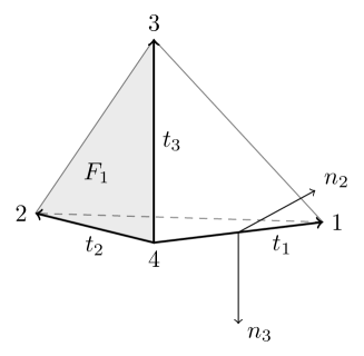
Unlike the traditional approach by transforming back to the reference element, we will chose an intrinsic coordinate. For ease of presentation, denote the four faces in (K)\mathcal{F}(K) by FiF_{i}, which is opposite to the iith vertex of KK, and by 𝒏i\boldsymbol{n}_{i} the outward unit normal vector of FiF_{i} for i=1,2,3,4i=1,2,3,4. Let 𝒕i\boldsymbol{t}_{i} be the unit tangential vector of the edge from vertex 44 to vertex ii; see Fig. 2. The set of three vectors {𝒕1,𝒕2,𝒕3}\{\boldsymbol{t}_{1},\boldsymbol{t}_{2},\boldsymbol{t}_{3}\} forms a basis of 3\mathbb{R}^{3} although they may not be orthogonal in general. Consequently {𝒕i𝒕j}i,j=13\{\boldsymbol{t}_{i}\boldsymbol{t}_{j}^{\intercal}\}_{i,j=1}^{3} forms a basis of the second order tensor and (𝒕i,𝒏i)0(\boldsymbol{t}_{i},\boldsymbol{n}_{i})\neq 0 for i=1,2,3i=1,2,3.

Refer to caption
Figure 2. Local coordinate formed by three edge vectors.

Let λi(𝒙)\lambda_{i}(\boldsymbol{x}) be the iith barycentric coordinate with respect to the tetrahedron KK for i=1,2,3,4i=1,2,3,4. Then λi|Fi=0\lambda_{i}|_{F_{i}}=0 and λi=ci𝒏i\nabla\lambda_{i}=-c_{i}\boldsymbol{n}_{i} for some ci>0c_{i}>0.

Theorem 5.3.

The degrees of freedom (54)-(60) are unisolvent for 𝚺,k(K)\boldsymbol{\Sigma}_{\ell,k}(K).

Proof.

We first count the number of the degrees of freedom (54)-(60). Calculation of d.o.f. (59) can be found in (50). The number of d.o.f. (54)-(60) is

24+18(1)+2[(1)(2)+(+1)]\displaystyle 24+18(\ell-1)+2[(\ell-1)(\ell-2)+(\ell+1)\ell]
+16(k3k)4+16(1)(5+14)+12(1)\displaystyle\quad+\frac{1}{6}(k^{3}-k)-4+\frac{1}{6}\ell(\ell-1)(5\ell+14)+\frac{1}{2}\ell(\ell-1)
=\displaystyle= 16(53+362+67+36)+16(k3k),\displaystyle\frac{1}{6}(5\ell^{3}+36\ell^{2}+67\ell+36)+\frac{1}{6}(k^{3}-k),

which is same as dim𝚺,k(K)\dim\boldsymbol{\Sigma}_{\ell,k}(K) cf. (46).

Take any 𝝉𝚺,k(K)\boldsymbol{\tau}\in\boldsymbol{\Sigma}_{\ell,k}(K) and suppose all the degrees of freedom (54)-(60) vanish. We are going to prove the function 𝝉=0\boldsymbol{\tau}=0. Using the local coordinate sketched in Fig. 2, we can expand 𝝉\boldsymbol{\tau} as

𝝉=i,j=13τij𝒕i𝒕jwithτij=𝒏i𝝉𝒏j(𝒕i𝒏i)(𝒕j𝒏j).\boldsymbol{\tau}=\sum_{i,j=1}^{3}\tau_{ij}\boldsymbol{t}_{i}\boldsymbol{t}_{j}^{\intercal}\quad\textrm{with}\quad\tau_{ij}=\frac{\boldsymbol{n}_{i}^{\intercal}\boldsymbol{\tau}\boldsymbol{n}_{j}}{(\boldsymbol{t}_{i}^{\intercal}\boldsymbol{n}_{i})(\boldsymbol{t}_{j}^{\intercal}\boldsymbol{n}_{j})}.

As 𝝉\boldsymbol{\tau} is symmetric, τij=τji\tau_{ij}=\tau_{ji}. By (62), it follows

τii|Fi=𝒏i𝝉𝒏i|Fi=0,i=1,2,3.\tau_{ii}|_{F_{i}}=\boldsymbol{n}_{i}^{\intercal}\boldsymbol{\tau}\boldsymbol{n}_{i}|_{F_{i}}=0,\quad i=1,2,3.

Thus there exists q11(K)q_{\ell-1}\in\mathbb{P}_{\ell-1}(K) satisfying τii=λiq1\tau_{ii}=\lambda_{i}q_{\ell-1} for i=1,2,3i=1,2,3. Taking 𝝇=q1𝒏i𝒏i\boldsymbol{\varsigma}=q_{\ell-1}\boldsymbol{n}_{i}\boldsymbol{n}_{i}^{\intercal} in (64) will produce

(65) τii=0,i=1,2,3.\tau_{ii}=0,\quad i=1,2,3.

Namely the diagonal of 𝝉\boldsymbol{\tau} is zero. So far, in the chosen coordinate, 𝒏4𝝉𝒏4=0\boldsymbol{n}_{4}^{\intercal}\boldsymbol{\tau}\boldsymbol{n}_{4}=0 has no simple formulation and will be used later on.

On the other hand, from (61) we have ΠF1(𝝉𝒏1)H0(divF1,F1)\Pi_{F_{1}}(\boldsymbol{\tau}\boldsymbol{n}_{1})\in H_{0}(\operatorname{div}_{F_{1}},F_{1}). As 𝒏1𝝉𝒏1=τ11=0\boldsymbol{n}_{1}^{\intercal}\boldsymbol{\tau}\boldsymbol{n}_{1}=\tau_{11}=0 in KK cf. (65), it follows n1(𝒏1𝝉𝒏1)|F1=0\partial_{n_{1}}(\boldsymbol{n}_{1}^{\intercal}\boldsymbol{\tau}\boldsymbol{n}_{1})|_{F_{1}}=0. Therefore (63) becomes

2divF1(𝝉𝒏1)|F1=0.2\operatorname{div}_{F_{1}}(\boldsymbol{\tau}\boldsymbol{n}_{1})|_{F_{1}}=0.

Hence there exists q22(F1)q_{\ell-2}\in\mathbb{P}_{\ell-2}(F_{1}) such that 𝒏1×(𝝉𝒏1)=F1(bF1q2)\boldsymbol{n}_{1}\times(\boldsymbol{\tau}\boldsymbol{n}_{1})=\nabla_{F_{1}}(b_{F_{1}}q_{\ell-2}), where bF1b_{F_{1}} is the cubic bubble function on face F1F_{1}. Together with (60) and the fact divF1(𝒙2(F1))=2(F1)\operatorname{div}_{F_{1}}(\boldsymbol{x}\mathbb{P}_{\ell-2}(F_{1}))=\mathbb{P}_{\ell-2}(F_{1}), we get (𝒏1×(𝝉𝒏1))|F1=𝟎(\boldsymbol{n}_{1}\times(\boldsymbol{\tau}\boldsymbol{n}_{1}))|_{F_{1}}=\boldsymbol{0}. Thus (𝝉𝒏1)|F1=𝟎(\boldsymbol{\tau}\boldsymbol{n}_{1})|_{F_{1}}=\boldsymbol{0}. Then there exists 𝒒11(K;3)\boldsymbol{q}_{\ell-1}\in\mathbb{P}_{\ell-1}(K;\mathbb{R}^{3}) such that 𝝉𝒏1=λ1𝒒1\boldsymbol{\tau}\boldsymbol{n}_{1}=\lambda_{1}\boldsymbol{q}_{\ell-1}, combined with (64) yields 𝝉𝒏1=𝟎\boldsymbol{\tau}\boldsymbol{n}_{1}=\boldsymbol{0}. That is the first row of 𝝉\boldsymbol{\tau} is zero, i.e. τ11=τ12=τ13=0\tau_{11}=\tau_{12}=\tau_{13}=0.

By the symmetry, now 𝝉=2τ23sym(𝒕2𝒕3)\boldsymbol{\tau}=2\tau_{23}\operatorname{sym}(\boldsymbol{t}_{2}\boldsymbol{t}_{3}^{\intercal}). Multiplying 𝝉\boldsymbol{\tau} by 𝒏4\boldsymbol{n}_{4} from both sides and restricting to F4F_{4}, we have

τ23|F4=12𝒏4𝝉𝒏4(𝒕2𝒏4)(𝒕3𝒏4)|F4=0.\tau_{23}|_{F_{4}}=\frac{1}{2}\frac{\boldsymbol{n}_{4}^{\intercal}\boldsymbol{\tau}\boldsymbol{n}_{4}}{(\boldsymbol{t}_{2}^{\intercal}\boldsymbol{n}_{4})(\boldsymbol{t}_{3}^{\intercal}\boldsymbol{n}_{4})}|_{F_{4}}=0.

The denominator is non-zero as 𝒕2,𝒕3\boldsymbol{t}_{2},\boldsymbol{t}_{3} are non tangential vectors of face F4F_{4}. Again there exists q11(K)q_{\ell-1}\in\mathbb{P}_{\ell-1}(K) satisfying τ23=λ4q1\tau_{23}=\lambda_{4}q_{\ell-1}. Taking 𝝇=sym(𝒕2𝒕3)q1\boldsymbol{\varsigma}=\operatorname{sym}(\boldsymbol{t}_{2}\boldsymbol{t}_{3}^{\intercal})q_{\ell-1} in (64) gives τ23=0\tau_{23}=0. We thus have proved 𝝉=0\boldsymbol{\tau}=0 and consequently the unisolvence. ∎

Due to (57), it is arduous to figure out the explicit basis functions of 𝚺,k(K)\boldsymbol{\Sigma}_{\ell,k}(K), which are dual to the degrees of freedom (54)-(60). Alternatively we can hybridize the degrees of freedom (57), and use the basis functions of the standard Lagrange element [6].

5.2. Polynomial bubble function spaces and the bubble complex

Let

𝚺̊,k(K)\displaystyle\mathring{\boldsymbol{\Sigma}}_{\ell,k}(K) :={𝝉𝚺,k(K):all degrees of freedom (54)-(57) vanish}.\displaystyle:=\{\boldsymbol{\tau}\in\boldsymbol{\Sigma}_{\ell,k}(K):\textrm{all degrees of freedom\leavevmode\nobreak\ \eqref{Hdivdivfem3ddof1}-\eqref{Hdivdivfem3ddof4} vanish}\}.

Together with vanishing (58), we can conclude that divdiv𝝉=0\operatorname{div}\operatorname{div}\boldsymbol{\tau}=0. In view of Fig. 1 and Lemma 5.2, the last two set of d.o.f. (59)-(60) can be replaced by

(𝝉,𝝇)K𝝇𝚺̊,k(K)ker(divdiv),(\boldsymbol{\tau},\boldsymbol{\varsigma})_{K}\quad\forall\leavevmode\nobreak\ \boldsymbol{\varsigma}\in\mathring{\boldsymbol{\Sigma}}_{\ell,k}(K)\cap\ker(\operatorname{div}\operatorname{div}),

Next we give characterization of 𝚺̊,k(K)ker(divdiv)\mathring{\boldsymbol{\Sigma}}_{\ell,k}(K)\cap\ker(\operatorname{div}\operatorname{div}).

By the exactness of divdiv complex, if divdiv𝝉=0\operatorname{div}\operatorname{div}\boldsymbol{\tau}=0 and tr(𝝉)=0\operatorname*{tr}(\boldsymbol{\tau})=0, it is possible that 𝝉=symcurl𝝈\boldsymbol{\tau}=\operatorname{sym}\operatorname{curl}\boldsymbol{\sigma} for some 𝝈𝑩+1(symcurl,K;𝕋):=𝑯0(symcurl,K;𝕋)+1(K;𝕋)\boldsymbol{\sigma}\in\boldsymbol{B}_{\ell+1}(\operatorname{sym}\operatorname{curl},K;\mathbb{T}):=\boldsymbol{H}_{0}(\operatorname{sym}\operatorname{curl},K;\mathbb{T})\cap\mathbb{P}_{\ell+1}(K;\mathbb{T}). We will give an explicit characterization of 𝑩+1(symcurl,K;𝕋)\boldsymbol{B}_{\ell+1}(\operatorname{sym}\operatorname{curl},K;\mathbb{T}), show 𝚺̊,k(K)ker(divdiv)=symcurl𝑩+1(symcurl,K;𝕋)\mathring{\boldsymbol{\Sigma}}_{\ell,k}(K)\cap\ker(\operatorname{div}\operatorname{div})=\operatorname{sym}\operatorname{curl}\boldsymbol{B}_{\ell+1}(\operatorname{sym}\operatorname{curl},K;\mathbb{T}), and consequently get a set of computable and symmetric d.o.f..

We begin with a characterization of the trace of functions in 𝑯(symcurl,K;𝕋)\boldsymbol{H}(\operatorname{sym}\operatorname{curl},K;\mathbb{T}).

Lemma 5.4 (Green’s identity).

Let KK be a polyhedron, and let 𝛕𝐇1(K;𝕄)\boldsymbol{\tau}\in\boldsymbol{H}^{1}(K;\mathbb{M}) and 𝛔𝐇1(K;𝕊)\boldsymbol{\sigma}\in\boldsymbol{H}^{1}(K;\mathbb{S}). Then we have

(symcurl𝝉,𝝈)K=(𝝉,curl𝝈)K\displaystyle(\operatorname{sym}\operatorname{curl}\boldsymbol{\tau},\boldsymbol{\sigma})_{K}=(\boldsymbol{\tau},\operatorname{curl}\boldsymbol{\sigma})_{K} F(K)(symΠF(𝝉×𝒏)ΠF,ΠF𝝈ΠF)F\displaystyle-\sum_{F\in\mathcal{F}(K)}(\operatorname{sym}\Pi_{F}(\boldsymbol{\tau}\times\boldsymbol{n})\Pi_{F},\Pi_{F}\boldsymbol{\sigma}\Pi_{F})_{F}
F(K)(𝒏𝝉×𝒏,𝒏𝝈ΠF)F.\displaystyle-\sum_{F\in\mathcal{F}(K)}(\boldsymbol{n}\cdot\boldsymbol{\tau}\times\boldsymbol{n},\boldsymbol{n}\cdot\boldsymbol{\sigma}\Pi_{F})_{F}.
Proof.

As 𝝈\boldsymbol{\sigma} is symmetric,

(symcurl𝝉,𝝈)K\displaystyle(\operatorname{sym}\operatorname{curl}\boldsymbol{\tau},\boldsymbol{\sigma})_{K} =(curl𝝉,𝝈)K=(𝝉,curl𝝈)K(𝝉×𝒏,𝝈)K.\displaystyle=(\operatorname{curl}\boldsymbol{\tau},\boldsymbol{\sigma})_{K}=(\boldsymbol{\tau},\operatorname{curl}\boldsymbol{\sigma})_{K}-(\boldsymbol{\tau}\times\boldsymbol{n},\boldsymbol{\sigma})_{\partial K}.

On each face, we expand the boundary term

(𝝉×𝒏,𝝈)F=(ΠF(𝝉×𝒏)ΠF,ΠF𝝈ΠF)F+(𝒏𝝉×𝒏,𝒏𝝈ΠF)F.\displaystyle(\boldsymbol{\tau}\times\boldsymbol{n},\boldsymbol{\sigma})_{F}=(\Pi_{F}(\boldsymbol{\tau}\times\boldsymbol{n})\Pi_{F},\Pi_{F}\boldsymbol{\sigma}\Pi_{F})_{F}+(\boldsymbol{n}\cdot\boldsymbol{\tau}\times\boldsymbol{n},\boldsymbol{n}\cdot\boldsymbol{\sigma}\Pi_{F})_{F}.

Then we use the fact ΠF𝝈ΠF\Pi_{F}\boldsymbol{\sigma}\Pi_{F} is symmetric to arrive the desired identity. ∎

Based on the Green’s identity, we introduce the following trace operators for 𝑯(symcurl)\boldsymbol{H}(\operatorname{sym}\operatorname{curl}) space

  1. (1)

    tr1(𝝉):=ΠFsym(𝝉×𝒏)ΠF\operatorname*{tr}_{1}(\boldsymbol{\tau}):=\Pi_{F}\operatorname{sym}(\boldsymbol{\tau}\times\boldsymbol{n})\Pi_{F},

  2. (2)

    tr1(𝝉):=𝒏×sym(𝝉×𝒏)×𝒏\operatorname*{tr}_{1}^{\bot}(\boldsymbol{\tau}):=\boldsymbol{n}\times\operatorname{sym}(\boldsymbol{\tau}\times\boldsymbol{n})\times\boldsymbol{n},

  3. (3)

    tr2(𝝉):=𝒏𝝉×𝒏\operatorname*{tr}_{2}(\boldsymbol{\tau}):=\boldsymbol{n}\cdot\boldsymbol{\tau}\times\boldsymbol{n}.

Both tr1(𝝉)\operatorname*{tr}_{1}(\boldsymbol{\tau}) and tr1(𝝉)\operatorname*{tr}_{1}^{\bot}(\boldsymbol{\tau}) are symmetric tensors on each face and tr2(𝝉)\operatorname*{tr}_{2}(\boldsymbol{\tau}) is a vector function. Obviously tr1(𝝉)=0\operatorname*{tr}_{1}(\boldsymbol{\tau})=0 if and only if tr1(𝝉)=0\operatorname*{tr}_{1}^{\bot}(\boldsymbol{\tau})=0 as tr1(𝝉)\operatorname*{tr}_{1}^{\bot}(\boldsymbol{\tau}) is just a rotation of tr1(𝝉)\operatorname*{tr}_{1}(\boldsymbol{\tau}). Using the trace operators, 𝑯(symcurl)\boldsymbol{H}(\operatorname{sym}\operatorname{curl}) polynomial bubble function space can be defined as

𝑩+1(symcurl,K;𝕋):={\displaystyle\boldsymbol{B}_{\ell+1}(\operatorname{sym}\operatorname{curl},K;\mathbb{T}):=\{ 𝝉+1(K;𝕋):(𝒏𝝉×𝒏)|F=𝟎,\displaystyle\boldsymbol{\tau}\in\mathbb{P}_{\ell+1}(K;\mathbb{T}):(\boldsymbol{n}\cdot\boldsymbol{\tau}\times\boldsymbol{n})|_{F}=\boldsymbol{0},
(𝒏×sym(𝝉×𝒏)×𝒏)|F=𝟎F(K)}.\displaystyle(\boldsymbol{n}\times\operatorname{sym}(\boldsymbol{\tau}\times\boldsymbol{n})\times\boldsymbol{n})|_{F}=\boldsymbol{0}\quad\forall\leavevmode\nobreak\ F\in\mathcal{F}(K)\}.

We shall give an explicit characterization of 𝑩+1(symcurl,K;𝕋)\boldsymbol{B}_{\ell+1}(\operatorname{sym}\operatorname{curl},K;\mathbb{T}).

Lemma 5.5.

Let 𝛕𝐁+1(symcurl,K;𝕋)\boldsymbol{\tau}\in\boldsymbol{B}_{\ell+1}(\operatorname{sym}\operatorname{curl},K;\mathbb{T}). It holds

(66) 𝝉|e=𝟎e(K).\boldsymbol{\tau}|_{e}=\boldsymbol{0}\quad\forall\leavevmode\nobreak\ e\in\mathcal{E}(K).
Proof.

It is straightforward to verify (66) on the reference tetrahedron for which 𝒆=(1,0,0)\boldsymbol{e}=(1,0,0) and two normal vectors of the face containing 𝒆\boldsymbol{e} is 𝒏1=(1,0,0)\boldsymbol{n}_{1}=(1,0,0) and 𝒏2=(0,0,1)\boldsymbol{n}_{2}=(0,0,1). To avoid complicated transformation of trace operators, we provide a proof using an intrinsic basis of 𝕋\mathbb{T} on KK.

Take any edge e(K)e\in\mathcal{E}(K) with the tangential vector 𝒕\boldsymbol{t}. Let 𝒏1\boldsymbol{n}_{1} and 𝒏2\boldsymbol{n}_{2} be the unit outward normal vectors of two faces sharing edge ee. Set 𝒔i:=𝒕×𝒏i\boldsymbol{s}_{i}:=\boldsymbol{t}\times\boldsymbol{n}_{i} for i=1,2i=1,2. By direction computation, we get on edge ee for i=1,2i=1,2 that

𝒏i𝝉𝒕=(𝒏i𝝉×𝒏i)𝒔i=0,\boldsymbol{n}_{i}^{\intercal}\boldsymbol{\tau}\boldsymbol{t}=(\boldsymbol{n}_{i}\cdot\boldsymbol{\tau}\times\boldsymbol{n}_{i})\cdot\boldsymbol{s}_{i}=0,
𝒏i𝝉𝒔i=(𝒏i𝝉×𝒏i)𝒕=0,\boldsymbol{n}_{i}^{\intercal}\boldsymbol{\tau}\boldsymbol{s}_{i}=-(\boldsymbol{n}_{i}\cdot\boldsymbol{\tau}\times\boldsymbol{n}_{i})\cdot\boldsymbol{t}=0,
𝒕𝝉𝒕𝒔i𝝉𝒔i=2𝒕sym(𝝉×𝒏i)𝒔i=2𝒔i(𝒏i×sym(𝝉×𝒏i)×𝒏i)𝒕=0,\boldsymbol{t}^{\intercal}\boldsymbol{\tau}\boldsymbol{t}-\boldsymbol{s}_{i}^{\intercal}\boldsymbol{\tau}\boldsymbol{s}_{i}=2\boldsymbol{t}\cdot\operatorname{sym}(\boldsymbol{\tau}\times\boldsymbol{n}_{i})\cdot\boldsymbol{s}_{i}=2\boldsymbol{s}_{i}\cdot(\boldsymbol{n}_{i}\times\operatorname{sym}(\boldsymbol{\tau}\times\boldsymbol{n}_{i})\times\boldsymbol{n}_{i})\cdot\boldsymbol{t}=0,
𝒕𝝉𝒔i=𝒕sym(𝝉×𝒏i)𝒕=𝒔i(𝒏i×sym(𝝉×𝒏i)×𝒏i)𝒔i=0.\boldsymbol{t}^{\intercal}\boldsymbol{\tau}\boldsymbol{s}_{i}=-\boldsymbol{t}\cdot\operatorname{sym}(\boldsymbol{\tau}\times\boldsymbol{n}_{i})\cdot\boldsymbol{t}=\boldsymbol{s}_{i}\cdot(\boldsymbol{n}_{i}\times\operatorname{sym}(\boldsymbol{\tau}\times\boldsymbol{n}_{i})\times\boldsymbol{n}_{i})\cdot\boldsymbol{s}_{i}=0.

Both span{𝒔1,𝒔2}\textrm{span}\{\boldsymbol{s}_{1},\boldsymbol{s}_{2}\} and span{𝒏1,𝒏2}\textrm{span}\{\boldsymbol{n}_{1},\boldsymbol{n}_{2}\} form the same normal vector space of edge ee, then the last identity implies

𝒕𝝉𝒏i=0.\boldsymbol{t}^{\intercal}\boldsymbol{\tau}\boldsymbol{n}_{i}=0.

Then it is sufficient to prove the eight trace-free tensors

(67) 𝒏1𝒕,𝒏2𝒕,𝒏1𝒔1,𝒏2𝒔2,𝒕𝒏1,𝒕𝒏2,𝒕𝒕𝒔1𝒔1,𝒕𝒕𝒔2𝒔2\boldsymbol{n}_{1}\boldsymbol{t}^{\intercal},\;\boldsymbol{n}_{2}\boldsymbol{t}^{\intercal},\;\boldsymbol{n}_{1}\boldsymbol{s}_{1}^{\intercal},\;\boldsymbol{n}_{2}\boldsymbol{s}_{2}^{\intercal},\;\boldsymbol{t}\,\boldsymbol{n}_{1}^{\intercal},\;\boldsymbol{t}\,\boldsymbol{n}_{2}^{\intercal},\;\boldsymbol{t}\,\boldsymbol{t}^{\intercal}-\boldsymbol{s}_{1}\boldsymbol{s}_{1}^{\intercal},\;\boldsymbol{t}\,\boldsymbol{t}^{\intercal}-\boldsymbol{s}_{2}\boldsymbol{s}_{2}^{\intercal}

are linear independent. Assume there exist cic_{i}\in\mathbb{R}, i=1,,8i=1,\cdots,8 such that

c1𝒏1𝒕+c2𝒏2𝒕+c3𝒏1𝒔1+c4𝒏2𝒔2+c5𝒕𝒏1+c6𝒕𝒏2\displaystyle c_{1}\boldsymbol{n}_{1}\boldsymbol{t}^{\intercal}+c_{2}\boldsymbol{n}_{2}\boldsymbol{t}^{\intercal}+c_{3}\boldsymbol{n}_{1}\boldsymbol{s}_{1}^{\intercal}+c_{4}\boldsymbol{n}_{2}\boldsymbol{s}_{2}^{\intercal}+c_{5}\boldsymbol{t}\,\boldsymbol{n}_{1}^{\intercal}+c_{6}\boldsymbol{t}\,\boldsymbol{n}_{2}^{\intercal}
+c7(𝒕𝒕𝒔1𝒔1)+c8(𝒕𝒕𝒔2𝒔2)\displaystyle+c_{7}(\boldsymbol{t}\,\boldsymbol{t}^{\intercal}-\boldsymbol{s}_{1}\boldsymbol{s}_{1}^{\intercal})+c_{8}(\boldsymbol{t}\,\boldsymbol{t}^{\intercal}-\boldsymbol{s}_{2}\boldsymbol{s}_{2}^{\intercal}) =𝟎.\displaystyle=\boldsymbol{0}.

Multiplying the last equation by 𝒕\boldsymbol{t} from the right and left respectively, we obtain

c1𝒏1+c2𝒏2+(c7+c8)𝒕=𝟎,c5𝒏1+c6𝒏2+(c7+c8)𝒕=𝟎.c_{1}\boldsymbol{n}_{1}+c_{2}\boldsymbol{n}_{2}+(c_{7}+c_{8})\boldsymbol{t}=\boldsymbol{0},\quad c_{5}\boldsymbol{n}_{1}^{\intercal}+c_{6}\boldsymbol{n}_{2}^{\intercal}+(c_{7}+c_{8})\boldsymbol{t}^{\intercal}=\boldsymbol{0}.

Hence c1=c2=c5=c6=c7+c8=0c_{1}=c_{2}=c_{5}=c_{6}=c_{7}+c_{8}=0, which yields

c3𝒏1𝒔1+c4𝒏2𝒔2+c7(𝒔2𝒔2𝒔1𝒔1)=𝟎.c_{3}\boldsymbol{n}_{1}\boldsymbol{s}_{1}^{\intercal}+c_{4}\boldsymbol{n}_{2}\boldsymbol{s}_{2}^{\intercal}+c_{7}(\boldsymbol{s}_{2}\boldsymbol{s}_{2}^{\intercal}-\boldsymbol{s}_{1}\boldsymbol{s}_{1}^{\intercal})=\boldsymbol{0}.

Multiplying the last equation by 𝒏1\boldsymbol{n}_{1} from the right, it follows

(𝒔2𝒏1)(c4𝒏2+c7𝒔2)=𝟎.(\boldsymbol{s}_{2}\cdot\boldsymbol{n}_{1})(c_{4}\boldsymbol{n}_{2}+c_{7}\boldsymbol{s}_{2})=\boldsymbol{0}.

As a result c4=c7=0c_{4}=c_{7}=0, and then c3=0c_{3}=0. ∎

We write +1(K;𝕋)\mathbb{P}_{\ell+1}(K;\mathbb{T}) as +1(K)𝕋\mathbb{P}_{\ell+1}(K)\otimes\mathbb{T} and use the barycentric coordinate representation of a polynomial. That is a polynomial p+1(K)p\in\mathbb{P}_{\ell+1}(K) has a unique representation in terms of

(68) p=λ1α1λ2α2λ3α3λ4α4,i=14αi=+1,αi.p=\lambda_{1}^{\alpha_{1}}\lambda_{2}^{\alpha_{2}}\lambda_{3}^{\alpha_{3}}\lambda_{4}^{\alpha_{4}},\quad\sum_{i=1}^{4}\alpha_{i}=\ell+1,\alpha_{i}\in\mathbb{N}.

Lemma 5.5 implies that pp must contain a face bubble bF=λiλjλkb_{F}=\lambda_{i}\lambda_{j}\lambda_{k} where (i,j,k)(i,j,k) are three vertices of FF. Otherwise, if p=λiαiλjαj,αi+αj=+1p=\lambda_{i}^{\alpha_{i}}\lambda_{j}^{\alpha_{j}},\alpha_{i}+\alpha_{j}=\ell+1, then pp is not zero on the edge (i,j)(i,j).

We consider the subspace bF2(K)𝕋b_{F}\mathbb{P}_{\ell-2}(K)\otimes\mathbb{T} and identify its intersection with ker(tr)\ker(\operatorname*{tr}). Due to the face bubble bFb_{F}, the polynomial is zero on the other faces. So we only need to consider the trace on face FF. Without loss of generality, we can chose the coordinate s.t. nF=(0,0,1)n_{F}=(0,0,1). Chose the canonical basis of 𝕋\mathbb{T} associated to this coordinate. Then by direct calculation to find out ker(tr)𝕋\ker(\operatorname*{tr})\cap\mathbb{T} consists of

(001000000),(000001000), and (100010002).\begin{pmatrix}0&0&1\\ 0&0&0\\ 0&0&0\end{pmatrix},\begin{pmatrix}0&0&0\\ 0&0&1\\ 0&0&0\end{pmatrix},\text{ and }\begin{pmatrix}1&0&0\\ 0&1&0\\ 0&0&-2\end{pmatrix}.

Switch to an intrinsic basis, we obtain the following explicit characterization of 𝑩+1(symcurl,K;𝕋)\boldsymbol{B}_{\ell+1}(\operatorname{sym}\operatorname{curl},K;\mathbb{T}).

Lemma 5.6.

For each face FF, we chose two unit tangent vectors 𝐭1,𝐭2\boldsymbol{t}_{1},\boldsymbol{t}_{2} s.t. (𝐭1,𝐭2,𝐧F)(\boldsymbol{t}_{1},\boldsymbol{t}_{2},\boldsymbol{n}_{F}) forms an orthonormal basis of 3\mathbb{R}^{3}. Then

(69) 𝑩+1(symcurl,K;𝕋)=span{pbFψiF,p2(K),F(K),i=1,2,3},\boldsymbol{B}_{\ell+1}(\operatorname{sym}\operatorname{curl},K;\mathbb{T})={\rm span}\{pb_{F}\psi_{i}^{F},p\in\mathbb{P}_{\ell-2}(K),F\in\mathcal{F}(K),i=1,2,3\},

where the three bubble functions are:

ψ1F=𝒕1𝒏F,ψ2F=𝒕2𝒏F,ψ3F=𝒕1𝒕1+𝒕2𝒕22𝒏F𝒏F.\psi_{1}^{F}=\boldsymbol{t}_{1}\boldsymbol{n}_{F}^{\intercal},\quad\psi_{2}^{F}=\boldsymbol{t}_{2}\boldsymbol{n}_{F}^{\intercal},\quad\psi_{3}^{F}=\boldsymbol{t}_{1}\boldsymbol{t}_{1}^{\intercal}+\boldsymbol{t}_{2}\boldsymbol{t}_{2}^{\intercal}-2\boldsymbol{n}_{F}\boldsymbol{n}_{F}^{\intercal}.
Proof.

Using the formulae (18)-(19), by the direct calculation, we can easily show ψiFker(tr)𝕋\psi_{i}^{F}\in\ker(\operatorname*{tr})\cap\mathbb{T} for each face FF and i=1,2,3i=1,2,3. As dimker(tr)𝕋=3\dim\ker(\operatorname*{tr})\cap\mathbb{T}=3, we conclude that

ker(tr)(bF2(K)𝕋)=span{pbFψiF,p2(K),i=1,2,3}.\ker(\operatorname*{tr})\cap(b_{F}\mathbb{P}_{\ell-2}(K)\otimes\mathbb{T})={\rm span}\{pb_{F}\psi_{i}^{F},p\in\mathbb{P}_{\ell-2}(K),i=1,2,3\}.

By Lemma 5.5 we know that

ker(tr)(+1𝕋)=Fker(tr)(bF2(K)𝕋)\ker(\operatorname*{tr})\cap(\mathbb{P}_{\ell+1}\otimes\mathbb{T})=\cup_{F}\ker(\operatorname*{tr})\cap(b_{F}\mathbb{P}_{\ell-2}(K)\otimes\mathbb{T})

and thus (69) follows. ∎

We only give a generating set of the bubble function space as the 1212 constant matrices {ψ1F,ψ2F,ψ3F,F(K)},\{\psi_{1}^{F},\psi_{2}^{F},\psi_{3}^{F},F\in\mathcal{F}(K)\}, are not linear independent. Next we find out a basis from this generating set.

Lemma 5.7.

Let (i,j,k)(i,j,k) be three vertices of face FF and 2(F)={λiα1λjα2λkα3,α1+α2+α3=2,αi,i=1,2,3}\mathbb{P}_{\ell-2}(F)=\{\lambda_{i}^{\alpha_{1}}\lambda_{j}^{\alpha_{2}}\lambda_{k}^{\alpha_{3}},\alpha_{1}+\alpha_{2}+\alpha_{3}=\ell-2,\alpha_{i}\in\mathbb{N},i=1,2,3\}. Define 𝐁F,+1:=bF2(F)span{ψ1F,ψ2F,ψ3F}\boldsymbol{B}_{F,\ell+1}:=b_{F}\mathbb{P}_{\ell-2}(F)\otimes{\rm span}\{\psi_{1}^{F},\psi_{2}^{F},\psi_{3}^{F}\} and 𝐁K,+1=bK3(K)span{ψ1F,ψ2F,F(K)}\boldsymbol{B}_{K,\ell+1}=b_{K}\mathbb{P}_{\ell-3}(K)\otimes{\rm span}\{\psi_{1}^{F},\psi_{2}^{F},F\in\mathcal{F}(K)\}. Then

(70) 𝑩+1(symcurl,K;𝕋)=F(K)𝑩F,+1𝑩K,+1,\boldsymbol{B}_{\ell+1}(\operatorname{sym}\operatorname{curl},K;\mathbb{T})=\oplus_{F\in\mathcal{F}(K)}\boldsymbol{B}_{F,\ell+1}\oplus\boldsymbol{B}_{K,\ell+1},

and consequently

dim𝑩+1(symcurl,K;𝕋)=23(1)(2+5)=13(43+6210).\dim\boldsymbol{B}_{\ell+1}(\operatorname{sym}\operatorname{curl},K;\mathbb{T})=\frac{2}{3}\ell(\ell-1)(2\ell+5)=\frac{1}{3}(4\ell^{3}+6\ell^{2}-10\ell).
Proof.

The 1212 constant matrices {ψ1F,ψ2F,ψ3F,F(K)}\{\psi_{1}^{F},\psi_{2}^{F},\psi_{3}^{F},F\in\mathcal{F}(K)\} are not linear independent as dim𝕋=8\dim\mathbb{T}=8. Among them, {ψ1F,ψ2F,F(K)}\{\psi_{1}^{F},\psi_{2}^{F},F\in\mathcal{F}(K)\} forms a basis of 𝕋\mathbb{T} which can be proved as verifying the linear independence of (67) in Lemma 5.5 or see [15].

For each pbFpb_{F}, with p2(K)p\in\mathbb{P}_{\ell-2}(K), we can group into either bK3(K)b_{K}\mathbb{P}_{\ell-3}(K) or bF2(F)b_{F}\mathbb{P}_{\ell-2}(F) depending on if the polynomial p|Fp|_{F} is zero or not, respectively. That is, for one fixed face FF:

bF2(K)=bF2(F)bK3(K).b_{F}\mathbb{P}_{\ell-2}(K)=b_{F}\mathbb{P}_{\ell-2}(F)\oplus b_{K}\mathbb{P}_{\ell-3}(K).

The sum is direct in view of the barycentric representation (68) of a polynomial. Then coupled with {ψiF}\{\psi_{i}^{F}\}, we get the basis (70) of the bubble function space.

The dimension of 𝑩+1(symcurl,K;𝕋)\boldsymbol{B}_{\ell+1}(\operatorname{sym}\operatorname{curl},K;\mathbb{T}) is

43dim2(F)+8dim3(K)=13(43+6210),\displaystyle 4\cdot 3\cdot\dim\mathbb{P}_{\ell-2}(F)+8\dim\mathbb{P}_{\ell-3}(K)=\frac{1}{3}(4\ell^{3}+6\ell^{2}-10\ell),

as required. ∎

We then verify symcurl𝑩+1(symcurl,K;𝕋)𝚺̊,k(K)\operatorname{sym}\operatorname{curl}\boldsymbol{B}_{\ell+1}(\operatorname{sym}\operatorname{curl},K;\mathbb{T})\subset\mathring{\boldsymbol{\Sigma}}_{\ell,k}(K) by verifying all boundary d.o.f. are vanished.

Lemma 5.8.

Let 𝛕𝐁+1(symcurl,K;𝕋)\boldsymbol{\tau}\in\boldsymbol{B}_{\ell+1}(\operatorname{sym}\operatorname{curl},K;\mathbb{T}). Assume edge e(K)e\in\mathcal{E}(K) is shared by faces FiF_{i} and FjF_{j}. It holds 𝐧i(symcurl𝛕)𝐧j|e=0\boldsymbol{n}_{i}^{\intercal}(\operatorname{sym}\operatorname{curl}\boldsymbol{\tau})\boldsymbol{n}_{j}|_{e}=0.

Proof.

For the ease of notation, let 𝝈=symcurl𝝉\boldsymbol{\sigma}=\operatorname{sym}\operatorname{curl}\boldsymbol{\tau}. Suppose 𝝉=F(K)l=13qF,lbFψlF\boldsymbol{\tau}=\sum\limits_{F\in\mathcal{F}(K)}\sum\limits_{l=1}^{3}q_{F,l}b_{F}\psi_{l}^{F} with qF,l2(K)q_{F,l}\in\mathbb{P}_{\ell-2}(K). By bF|e=0b_{F}|_{e}=0, we get

𝒏i𝝈𝒏j|e=F(K)l=13qF,l|e(𝒏isymcurl(bFψlF)𝒏j)|e.\boldsymbol{n}_{i}^{\intercal}\boldsymbol{\sigma}\boldsymbol{n}_{j}|_{e}=\sum_{F\in\mathcal{F}(K)}\sum_{l=1}^{3}q_{F,l}|_{e}(\boldsymbol{n}_{i}^{\intercal}\operatorname{sym}\operatorname{curl}(b_{F}\psi_{l}^{F})\boldsymbol{n}_{j})|_{e}.

Since λi|e=λj|e=0\lambda_{i}|_{e}=\lambda_{j}|_{e}=0, we can see that (𝒏i×𝒏FbF)|e=(𝒏j×𝒏FbF)|e=0(\boldsymbol{n}_{i}\times\boldsymbol{n}_{F}\cdot\nabla b_{F})|_{e}=(\boldsymbol{n}_{j}\times\boldsymbol{n}_{F}\cdot\nabla b_{F})|_{e}=0. Thus for l=1,2l=1,2,

(𝒏isymcurl(bFψlF)𝒏j)|e\displaystyle\quad\;(\boldsymbol{n}_{i}^{\intercal}\operatorname{sym}\operatorname{curl}(b_{F}\psi_{l}^{F})\boldsymbol{n}_{j})|_{e}
=(𝒏i(bF𝒕l𝒏F)×𝒏j)|e(𝒏j(bF𝒕l𝒏F)×𝒏i)|e\displaystyle=-(\boldsymbol{n}_{i}\cdot(b_{F}\boldsymbol{t}_{l}\boldsymbol{n}_{F})\times\nabla\cdot\boldsymbol{n}_{j})|_{e}-(\boldsymbol{n}_{j}\cdot(b_{F}\boldsymbol{t}_{l}\boldsymbol{n}_{F})\times\nabla\cdot\boldsymbol{n}_{i})|_{e}
=𝒏i𝒕l(𝒏F×𝒏jbF)|e+𝒏j𝒕l(𝒏F×𝒏ibF)|e\displaystyle=\boldsymbol{n}_{i}\cdot\boldsymbol{t}_{l}(\boldsymbol{n}_{F}\times\boldsymbol{n}_{j}\cdot\nabla b_{F})|_{e}+\boldsymbol{n}_{j}\cdot\boldsymbol{t}_{l}(\boldsymbol{n}_{F}\times\boldsymbol{n}_{i}\cdot\nabla b_{F})|_{e}
=0.\displaystyle=0.

Next consider l=3l=3. When FFjF\neq F_{j}, the face bubble bFb_{F} has a factor λj\lambda_{j}, which implies (𝒏j×bF)|e=𝟎(\boldsymbol{n}_{j}\times\nabla b_{F})|_{e}=\boldsymbol{0}. Thus

(𝒏icurl(bFψ3F)𝒏j)|e=(𝒏i(bFψ3F)×𝒏j)|e=(𝒏iψ3F(𝒏j×bF))|e=0.(\boldsymbol{n}_{i}^{\intercal}\operatorname{curl}(b_{F}\psi_{3}^{F})\boldsymbol{n}_{j})|_{e}=-(\boldsymbol{n}_{i}\cdot(b_{F}\psi_{3}^{F})\times\nabla\cdot\boldsymbol{n}_{j})|_{e}=(\boldsymbol{n}_{i}\cdot\psi_{3}^{F}\cdot(\boldsymbol{n}_{j}\times\nabla b_{F}))|_{e}=0.

When F=FjF=F_{j}, the face bubble bFb_{F} has a factor λi\lambda_{i}. By the fact that (𝒕1,𝒕2,𝒏j)(\boldsymbol{t}_{1},\boldsymbol{t}_{2},\boldsymbol{n}_{j}) forms an orthonormal basis of 3\mathbb{R}^{3},

𝒏i𝒕2(𝒕2×𝒏jλi)\displaystyle\boldsymbol{n}_{i}\cdot\boldsymbol{t}_{2}(\boldsymbol{t}_{2}\times\boldsymbol{n}_{j}\cdot\nabla\lambda_{i}) =𝒏i(𝒏j×𝒕1)(𝒕1λi)=(𝒕1λi)(𝒏j×𝒏i𝒕1)\displaystyle=\boldsymbol{n}_{i}\cdot(\boldsymbol{n}_{j}\times\boldsymbol{t}_{1})(\boldsymbol{t}_{1}\cdot\nabla\lambda_{i})=-(\boldsymbol{t}_{1}\cdot\nabla\lambda_{i})(\boldsymbol{n}_{j}\times\boldsymbol{n}_{i}\cdot\boldsymbol{t}_{1})
=𝒏i𝒕1(𝒏j×λi𝒕1),\displaystyle=-\boldsymbol{n}_{i}\cdot\boldsymbol{t}_{1}(\boldsymbol{n}_{j}\times\nabla\lambda_{i}\cdot\boldsymbol{t}_{1}),

which implies

𝒏i𝒕1(𝒏j×λi𝒕1)+𝒏i𝒕2(𝒏j×λi𝒕2)=0.\boldsymbol{n}_{i}\cdot\boldsymbol{t}_{1}(\boldsymbol{n}_{j}\times\nabla\lambda_{i}\cdot\boldsymbol{t}_{1})+\boldsymbol{n}_{i}\cdot\boldsymbol{t}_{2}(\boldsymbol{n}_{j}\times\nabla\lambda_{i}\cdot\boldsymbol{t}_{2})=0.

As a result,

(𝒏icurl(bFψ3F)𝒏j)|e=𝒏i𝒕1(𝒏j×bF𝒕1)|e+𝒏i𝒕2(𝒏j×bF𝒕2)|e=0.(\boldsymbol{n}_{i}^{\intercal}\operatorname{curl}(b_{F}\psi_{3}^{F})\boldsymbol{n}_{j})|_{e}=\boldsymbol{n}_{i}\cdot\boldsymbol{t}_{1}(\boldsymbol{n}_{j}\times\nabla b_{F}\cdot\boldsymbol{t}_{1})|_{e}+\boldsymbol{n}_{i}\cdot\boldsymbol{t}_{2}(\boldsymbol{n}_{j}\times\nabla b_{F}\cdot\boldsymbol{t}_{2})|_{e}=0.

Similarly (𝒏jcurl(bFψ3F)𝒏i)|e=0(\boldsymbol{n}_{j}^{\intercal}\operatorname{curl}(b_{F}\psi_{3}^{F})\boldsymbol{n}_{i})|_{e}=0 holds. Hence (𝒏isymcurl(bFψ3F)𝒏j)|e=0(\boldsymbol{n}_{i}^{\intercal}\operatorname{sym}\operatorname{curl}(b_{F}\psi_{3}^{F})\boldsymbol{n}_{j})|_{e}=0.

Therefore 𝒏i𝝈𝒏j|e=0\boldsymbol{n}_{i}^{\intercal}\boldsymbol{\sigma}\boldsymbol{n}_{j}|_{e}=0. ∎

Next we show the two traces tr2(𝝉)\operatorname*{tr}_{2}(\boldsymbol{\tau}) is in H(divF)H(\operatorname{div}_{F}) and tr1(𝝉)\operatorname*{tr}_{1}(\boldsymbol{\tau}) in H(divFdivF)H(\operatorname{div}_{F}\operatorname{div}_{F}).

Lemma 5.9.

When 𝛔=symcurl𝛕\boldsymbol{\sigma}=\operatorname{sym}\operatorname{curl}\,\boldsymbol{\tau} with 𝛕𝐇2(K;𝕄)\boldsymbol{\tau}\in\boldsymbol{H}^{2}(K;\mathbb{M}), we can express the trace in terms of the differential operators on surface FF of KK

(71) 𝒏𝝈𝒏\displaystyle\boldsymbol{n}^{\intercal}\boldsymbol{\sigma}\boldsymbol{n} =divF(𝒏𝝉×𝒏),\displaystyle=\operatorname{div}_{F}(\boldsymbol{n}\cdot\boldsymbol{\tau}\times\boldsymbol{n}),
(72) F(𝒏×𝝈𝒏)+𝒏div𝝈\displaystyle\nabla_{F}^{\bot}\cdot(\boldsymbol{n}\times\boldsymbol{\sigma}\cdot\boldsymbol{n})+\boldsymbol{n}^{\intercal}\operatorname{div}\boldsymbol{\sigma} =rotFrotF(𝒏×sym(𝝉×𝒏)×𝒏)\displaystyle=-\mathrm{rot}_{F}\mathrm{rot}_{F}(\boldsymbol{n}\times\operatorname{sym}(\boldsymbol{\tau}\times\boldsymbol{n})\times\boldsymbol{n})
=divFdivF(ΠFsym(𝝉×𝒏)ΠF).\displaystyle=\operatorname{div}_{F}\operatorname{div}_{F}(\Pi_{F}\operatorname{sym}(\boldsymbol{\tau}\times\boldsymbol{n})\Pi_{F}).
Proof.

By

𝒏𝝈𝒏\displaystyle\boldsymbol{n}^{\intercal}\boldsymbol{\sigma}\boldsymbol{n} =12𝒏(×(𝝉)𝝉×)𝒏=12F(𝝉)𝒏+12𝒏𝝉F\displaystyle=\frac{1}{2}\boldsymbol{n}\cdot(\nabla\times(\boldsymbol{\tau}^{\intercal})-\boldsymbol{\tau}\times\nabla)\cdot\boldsymbol{n}=\frac{1}{2}\nabla_{F}^{\bot}\cdot(\boldsymbol{\tau}^{\intercal})\cdot\boldsymbol{n}+\frac{1}{2}\boldsymbol{n}\cdot\boldsymbol{\tau}\cdot\nabla_{F}^{\bot}

and the fact F(𝝉)𝒏=𝒏𝝉F\nabla_{F}^{\bot}\cdot(\boldsymbol{\tau}^{\intercal})\cdot\boldsymbol{n}=\boldsymbol{n}\cdot\boldsymbol{\tau}\cdot\nabla_{F}^{\bot}, we get

𝒏𝝈𝒏=𝒏𝝉F=rotF(𝒏𝝉ΠF).\boldsymbol{n}^{\intercal}\boldsymbol{\sigma}\boldsymbol{n}=\boldsymbol{n}\cdot\boldsymbol{\tau}\cdot\nabla_{F}^{\bot}=\mathrm{rot}_{F}(\boldsymbol{n}\cdot\boldsymbol{\tau}\Pi_{F}).

Then the identity (71) holds from (26).

Next we prove (72). Employing (25) with 𝒗=𝝉𝒏\boldsymbol{v}=\boldsymbol{\tau}^{\intercal}\cdot\boldsymbol{n},

F(𝒏×𝝈𝒏)\displaystyle\nabla_{F}^{\bot}\cdot(\boldsymbol{n}\times\boldsymbol{\sigma}\cdot\boldsymbol{n}) =12F(𝒏×(×(𝝉)𝝉×)𝒏)\displaystyle=\frac{1}{2}\nabla_{F}^{\bot}\cdot\big{(}\boldsymbol{n}\times(\nabla\times(\boldsymbol{\tau}^{\intercal})-\boldsymbol{\tau}\times\nabla)\cdot\boldsymbol{n}\big{)}
=12F(𝒏×(×(𝝉𝒏)))+12F(𝒏×𝝉)F\displaystyle=\frac{1}{2}\nabla_{F}^{\bot}\cdot\big{(}\boldsymbol{n}\times(\nabla\times(\boldsymbol{\tau}^{\intercal}\cdot\boldsymbol{n}))\big{)}+\frac{1}{2}\nabla_{F}^{\bot}\cdot(\boldsymbol{n}\times\boldsymbol{\tau})\cdot\nabla_{F}^{\bot}
=12F((𝒏𝝉𝒏)n(𝝉𝒏))+12F(𝒏×𝝉)F\displaystyle=\frac{1}{2}\nabla_{F}^{\bot}\cdot\big{(}\nabla(\boldsymbol{n}\cdot\boldsymbol{\tau}^{\intercal}\cdot\boldsymbol{n})-\partial_{n}(\boldsymbol{\tau}^{\intercal}\cdot\boldsymbol{n})\big{)}+\frac{1}{2}\nabla_{F}^{\bot}\cdot(\boldsymbol{n}\times\boldsymbol{\tau})\cdot\nabla_{F}^{\bot}
=12F(n(𝝉𝒏))+12F(𝒏×𝝉)F.\displaystyle=-\frac{1}{2}\nabla_{F}^{\bot}\cdot\big{(}\partial_{n}(\boldsymbol{\tau}^{\intercal}\cdot\boldsymbol{n})\big{)}+\frac{1}{2}\nabla_{F}^{\bot}\cdot(\boldsymbol{n}\times\boldsymbol{\tau})\cdot\nabla_{F}^{\bot}.

On the other side, we have

𝒏div𝝈\displaystyle\boldsymbol{n}\cdot\operatorname{div}\boldsymbol{\sigma} =𝒏𝝈=12𝒏(×(𝝉))=12F(𝝉)\displaystyle=\boldsymbol{n}\cdot\boldsymbol{\sigma}\cdot\nabla=\frac{1}{2}\boldsymbol{n}\cdot(\nabla\times(\boldsymbol{\tau}^{\intercal}))\cdot\nabla=\frac{1}{2}\nabla_{F}^{\bot}\cdot(\boldsymbol{\tau}^{\intercal})\cdot\nabla
=12F(𝝉)(𝒏n+F)=12F(n(𝝉𝒏))+12F(𝝉)F\displaystyle=\frac{1}{2}\nabla_{F}^{\bot}\cdot(\boldsymbol{\tau}^{\intercal})\cdot(\boldsymbol{n}\partial_{n}+\nabla_{F})=\frac{1}{2}\nabla_{F}^{\bot}\cdot\big{(}\partial_{n}(\boldsymbol{\tau}^{\intercal}\cdot\boldsymbol{n})\big{)}+\frac{1}{2}\nabla_{F}^{\bot}\cdot(\boldsymbol{\tau}^{\intercal})\cdot\nabla_{F}
=12F(n(𝝉𝒏))12F(𝝉×𝒏)F.\displaystyle=\frac{1}{2}\nabla_{F}^{\bot}\cdot\big{(}\partial_{n}(\boldsymbol{\tau}^{\intercal}\cdot\boldsymbol{n})\big{)}-\frac{1}{2}\nabla_{F}^{\bot}\cdot(\boldsymbol{\tau}^{\intercal}\times\boldsymbol{n})\cdot\nabla_{F}^{\bot}.

The sum of the last two identities gives

F(𝒏×𝝈𝒏)+𝒏div𝝈\displaystyle\nabla_{F}^{\bot}\cdot(\boldsymbol{n}\times\boldsymbol{\sigma}\cdot\boldsymbol{n})+\boldsymbol{n}\cdot\operatorname{div}\boldsymbol{\sigma} =Fsym(𝒏×𝝉ΠF)F.\displaystyle=\nabla_{F}^{\bot}\cdot\operatorname{sym}(\boldsymbol{n}\times\boldsymbol{\tau}\Pi_{F})\cdot\nabla_{F}^{\bot}.

Therefore (72) follows from sym(𝒏×𝝉ΠF)=𝒏×sym(𝝉×𝒏)×𝒏\operatorname{sym}(\boldsymbol{n}\times\boldsymbol{\tau}\Pi_{F})=-\boldsymbol{n}\times\operatorname{sym}(\boldsymbol{\tau}\times\boldsymbol{n})\times\boldsymbol{n}. ∎

Note that F(𝒏×𝝈𝒏)+𝒏div𝝈\nabla_{F}^{\bot}\cdot(\boldsymbol{n}\times\boldsymbol{\sigma}\cdot\boldsymbol{n})+\boldsymbol{n}^{\intercal}\operatorname{div}\boldsymbol{\sigma} is an equivalent formulation of the second trace of 𝝈\boldsymbol{\sigma}. Combining Lemmas 5.8 and 5.9 gives the following result.

Lemma 5.10.

It holds

(73) symcurl𝑩+1(symcurl,K;𝕋)(𝚺̊,k(K)ker(divdiv)).\operatorname{sym}\operatorname{curl}\boldsymbol{B}_{\ell+1}(\operatorname{sym}\operatorname{curl},K;\mathbb{T})\subseteq(\mathring{\boldsymbol{\Sigma}}_{\ell,k}(K)\cap\ker(\operatorname{div}\operatorname{div})).
Proof.

For 𝝉𝑩+1(symcurl,K;𝕋)\boldsymbol{\tau}\in\boldsymbol{B}_{\ell+1}(\operatorname{sym}\operatorname{curl},K;\mathbb{T}), by construction, 𝒏𝝉×𝒏=0\boldsymbol{n}\cdot\boldsymbol{\tau}\times\boldsymbol{n}=0 and 𝒏×sym(𝝉×𝒏)×𝒏=0\boldsymbol{n}\times\operatorname{sym}(\boldsymbol{\tau}\times\boldsymbol{n})\times\boldsymbol{n}=0 on K\partial K. Let 𝝈=symcurl𝝉\boldsymbol{\sigma}=\operatorname{sym}\operatorname{curl}\boldsymbol{\tau}. Then by Lemma 5.9, d.o.f. (56)-(57) vanish. By Lemma 5.8, (55) vanish. As 𝝉\boldsymbol{\tau} contains a face bubble, 𝝈\boldsymbol{\sigma} will have an edge bubble function which means 𝝈(δ)=0\boldsymbol{\sigma}(\delta)=0 for all δ𝒱(K)\delta\in\mathcal{V}(K). Therefore symcurl𝑩+1(symcurl,K;𝕋)𝚺̊,k(K)\operatorname{sym}\operatorname{curl}\boldsymbol{B}_{\ell+1}(\operatorname{sym}\operatorname{curl},K;\mathbb{T})\subseteq\mathring{\boldsymbol{\Sigma}}_{\ell,k}(K). The property divdiv(symcurl𝝉)=0\operatorname{div}\operatorname{div}(\operatorname{sym}\operatorname{curl}\boldsymbol{\tau})=0 is from the divdiv complex. ∎

Indeed the ``"``\subseteq" in (73) can be changed to “=”. This will be clean after we present a bubble complex.

Lemma 5.11.

For each K𝒯hK\in\mathcal{T}_{h}, it holds

(74) divdiv𝚺̊,k(K)=k2(K)1(K),\operatorname{div}\operatorname{div}\mathring{\boldsymbol{\Sigma}}_{\ell,k}(K)=\mathbb{P}_{k-2}(K)\cap\mathbb{P}_{1}^{\bot}(K),

where 1(K)\mathbb{P}_{1}^{\bot}(K) is a subspace of L2(K)L^{2}(K) being orthogonal to 1(K)\mathbb{P}_{1}(K) with respect to the L2L^{2}-inner product (,)K(\cdot,\cdot)_{K}. Consequently

(75) dim(𝚺̊,k(K)ker(divdiv))=16(1)(5+17).\dim(\mathring{\boldsymbol{\Sigma}}_{\ell,k}(K)\cap\ker(\operatorname{div}\operatorname{div}))=\frac{1}{6}\ell(\ell-1)(5\ell+17).
Proof.

From the integration by parts, it is obviously true that divdiv𝚺̊,k(K)k2(K)1(K)\operatorname{div}\operatorname{div}\mathring{\boldsymbol{\Sigma}}_{\ell,k}(K)\subseteq\mathbb{P}_{k-2}(K)\cap\mathbb{P}_{1}^{\bot}(K). On the other side, for any vk2(K)1(K)v\in\mathbb{P}_{k-2}(K)\cap\mathbb{P}_{1}^{\bot}(K), due to the fact that divdiv𝑯02(K;𝕊)=L2(K)1(K)\operatorname{div}\operatorname{div}\boldsymbol{H}_{0}^{2}(K;\mathbb{S})=L^{2}(K)\cap\mathbb{P}_{1}^{\bot}(K) [10], there exists 𝝉~𝑯02(K;𝕊)\widetilde{\boldsymbol{\tau}}\in\boldsymbol{H}_{0}^{2}(K;\mathbb{S}) such that

divdiv𝝉~=v.\operatorname{div}\operatorname{div}\widetilde{\boldsymbol{\tau}}=v.

Then take 𝝉𝚺̊,k(K)\boldsymbol{\tau}\in\mathring{\boldsymbol{\Sigma}}_{\ell,k}(K) with the rest d.o.f.

(𝝉𝝉~,𝝇)K=0\displaystyle(\boldsymbol{\tau}-\widetilde{\boldsymbol{\tau}},\boldsymbol{\varsigma})_{K}=0 𝝇2k2(K)sym(2(K;𝕋)×𝒙),\displaystyle\quad\forall\leavevmode\nobreak\ \boldsymbol{\varsigma}\in\nabla^{2}\mathbb{P}_{k-2}(K)\oplus\operatorname{sym}(\mathbb{P}_{\ell-2}(K;\mathbb{T})\times\boldsymbol{x}),
((𝝉𝝉~)𝒏,𝒏×𝒙q)F1=0\displaystyle((\boldsymbol{\tau}-\widetilde{\boldsymbol{\tau}})\boldsymbol{n},\boldsymbol{n}\times\boldsymbol{x}q)_{F_{1}}=0 q2(F1).\displaystyle\quad\forall\leavevmode\nobreak\ q\in\mathbb{P}_{\ell-2}(F_{1}).

Applying the Green’s identity (53), we get

(divdiv(𝝉𝝉~),q)K=0qk2(K).(\operatorname{div}\operatorname{div}(\boldsymbol{\tau}-\widetilde{\boldsymbol{\tau}}),q)_{K}=0\quad\forall\leavevmode\nobreak\ q\in\mathbb{P}_{k-2}(K).

This implies divdiv𝝉=divdiv𝝉~=v\operatorname{div}\operatorname{div}\boldsymbol{\tau}=\operatorname{div}\operatorname{div}\widetilde{\boldsymbol{\tau}}=v. Namely (74) holds.

An immediate result of (74) is

dim(𝚺̊,k(K)ker(divdiv))\displaystyle\dim(\mathring{\boldsymbol{\Sigma}}_{\ell,k}(K)\cap\ker(\operatorname{div}\operatorname{div})) =dim𝚺̊,k(K)dimk2(K)+4\displaystyle=\dim\mathring{\boldsymbol{\Sigma}}_{\ell,k}(K)-\dim\mathbb{P}_{k-2}(K)+4
=16(1)(5+14)+12(1)\displaystyle=\frac{1}{6}\ell(\ell-1)(5\ell+14)+\frac{1}{2}\ell(\ell-1)
=16(1)(5+17).\displaystyle=\frac{1}{6}\ell(\ell-1)(5\ell+17).

Define

𝑩+2(K;3):={𝒗+2(K;3):𝒗|K=𝟎}=bK2(K;3).\boldsymbol{B}_{\ell+2}(K;\mathbb{R}^{3}):=\{\boldsymbol{v}\in\mathbb{P}_{\ell+2}(K;\mathbb{R}^{3}):\boldsymbol{v}|_{\partial K}=\boldsymbol{0}\}=b_{K}\mathbb{P}_{\ell-2}(K;\mathbb{R}^{3}).

Now we are in the position to present the so-called bubble complex.

Theorem 5.12.

The bubble function spaces for the divdiv complex

(76)

0𝑩+2(K;3)devgrad𝑩+1(symcurl,K;𝕋)symcurl𝚺̊,k(K)divdivk2(K)1(K)00\xrightarrow{}\boldsymbol{B}_{\ell+2}(K;\mathbb{R}^{3})\xrightarrow{\operatorname{dev}\operatorname{grad}}\boldsymbol{B}_{\ell+1}(\operatorname{sym}\operatorname{curl},K;\mathbb{T})\xrightarrow{\operatorname{sym}\operatorname{curl}}\mathring{\boldsymbol{\Sigma}}_{\ell,k}(K)\xrightarrow{\operatorname{div}{\operatorname{div}}}\mathbb{P}_{k-2}(K)\cap\mathbb{P}_{1}^{\bot}(K)\xrightarrow{}0

form an exact Hilbert complex.

Proof.

Take any 𝒗𝑩+2(K;3)\boldsymbol{v}\in\boldsymbol{B}_{\ell+2}(K;\mathbb{R}^{3}) with 𝒗|K=𝟎\boldsymbol{v}|_{\partial K}=\boldsymbol{0}. We have on each face F(K)F\in\mathcal{F}(K),

(77) 𝒏(devgrad𝒗)×𝒏=𝒏(grad𝒗)×𝒏=(𝒏×)(𝒗𝒏)=𝟎,\boldsymbol{n}\cdot(\operatorname{dev}\operatorname{grad}\boldsymbol{v})\times\boldsymbol{n}=\boldsymbol{n}\cdot(\operatorname{grad}\boldsymbol{v})\times\boldsymbol{n}=-(\boldsymbol{n}\times\nabla)(\boldsymbol{v}\cdot\boldsymbol{n})=\boldsymbol{0},

and

𝒏×sym((devgrad𝒗)×𝒏)×𝒏\displaystyle\boldsymbol{n}\times\operatorname{sym}((\operatorname{dev}\operatorname{grad}\boldsymbol{v})\times\boldsymbol{n})\times\boldsymbol{n} =𝒏×sym((grad𝒗)×𝒏)×𝒏\displaystyle=\boldsymbol{n}\times\operatorname{sym}((\operatorname{grad}\boldsymbol{v})\times\boldsymbol{n})\times\boldsymbol{n}
=𝒏×sym(𝒗F)×𝒏\displaystyle=-\boldsymbol{n}\times\operatorname{sym}(\boldsymbol{v}\nabla_{F}^{\bot})\times\boldsymbol{n}
(78) =𝒏×sym((ΠF𝒗)F)×𝒏=𝟎.\displaystyle=-\boldsymbol{n}\times\operatorname{sym}((\Pi_{F}\boldsymbol{v})\nabla_{F}^{\bot})\times\boldsymbol{n}=\boldsymbol{0}.

Hence devgrad𝑩+2(K;3)𝑩+1(symcurl,K;𝕋)ker(symcurl)\operatorname{dev}\operatorname{grad}\boldsymbol{B}_{\ell+2}(K;\mathbb{R}^{3})\subseteq\boldsymbol{B}_{\ell+1}(\operatorname{sym}\operatorname{curl},K;\mathbb{T})\cap\ker(\operatorname{sym}\operatorname{curl}). Thanks to Lemma 5.10 and (74), we conclude that  (76) is a complex.

We then verify the exactness from the left to the right.

1. 𝐁+1(symcurl,K;𝕋)ker(symcurl)=devgrad𝐁+2(K;3)\boldsymbol{B}_{\ell+1}(\operatorname{sym}\operatorname{curl},K;\mathbb{T})\cap\ker(\operatorname{sym}\operatorname{curl})=\operatorname{dev}\operatorname{grad}\boldsymbol{B}_{\ell+2}(K;\mathbb{R}^{3}), i.e. if symcurl𝛕=𝟎\operatorname{sym}\operatorname{curl}\boldsymbol{\tau}=\boldsymbol{0} and 𝛕𝐁+1(symcurl,K;𝕋)\boldsymbol{\tau}\in\boldsymbol{B}_{\ell+1}(\operatorname{sym}\operatorname{curl},K;\mathbb{T}), then there exists a 𝐯𝐁+2(K;3)\boldsymbol{v}\in\boldsymbol{B}_{\ell+2}(K;\mathbb{R}^{3}), s.t. 𝛕=devgrad𝐯\boldsymbol{\tau}=\operatorname{dev}\operatorname{grad}\boldsymbol{v}.

Firstly, by the exactness of the polynomial divdiv complex (33), there exists 𝒗+2(K;3)\boldsymbol{v}\in\mathbb{P}_{\ell+2}(K;\mathbb{R}^{3}) such that 𝝉=devgrad𝒗\boldsymbol{\tau}=\operatorname{dev}\operatorname{grad}\boldsymbol{v}. As 𝑹𝑻=ker(devgrad)\boldsymbol{RT}=\ker(\operatorname{dev}\operatorname{grad}), we can further impose constraint F𝒗𝒏=0\int_{F}\boldsymbol{v}\cdot\boldsymbol{n}=0 for each F(K)F\in\mathcal{F}(K). By (77), we get 𝒗𝒏F0(F)\boldsymbol{v}\cdot\boldsymbol{n}\mid_{F}\in\mathbb{P}_{0}(F). Hence 𝒗𝒏|F=0\boldsymbol{v}\cdot\boldsymbol{n}|_{F}=0, which indicates 𝒗(δ)=𝟎\boldsymbol{v}(\delta)=\boldsymbol{0} for each vertex δ𝒱(K)\delta\in\mathcal{V}(K). By (78), we obtain sym((ΠF𝒗)F)=𝟎\operatorname{sym}((\Pi_{F}\boldsymbol{v})\nabla_{F}^{\bot})=\boldsymbol{0}, i.e. ΠF𝒗0(F;2)+(ΠF𝒙)0(F)\Pi_{F}\boldsymbol{v}\in\mathbb{P}_{0}(F;\mathbb{R}^{2})+(\Pi_{F}\boldsymbol{x})\mathbb{P}_{0}(F). This combined with 𝒗(δ)=𝟎\boldsymbol{v}(\delta)=\boldsymbol{0} for each vertex δ𝒱(F)\delta\in\mathcal{V}(F) means ΠF𝒗=𝟎\Pi_{F}\boldsymbol{v}=\boldsymbol{0}, and then 𝒗|F=𝟎\boldsymbol{v}|_{F}=\boldsymbol{0} for each F(K)F\in\mathcal{F}(K). Thus 𝒗𝑩+2(K;3)\boldsymbol{v}\in\boldsymbol{B}_{\ell+2}(K;\mathbb{R}^{3}).

2. symcurl𝐁+1(symcurl,K;𝕋)=𝚺̊,k(K)ker(divdiv)\operatorname{sym}\operatorname{curl}\boldsymbol{B}_{\ell+1}(\operatorname{sym}\operatorname{curl},K;\mathbb{T})=\mathring{\boldsymbol{\Sigma}}_{\ell,k}(K)\cap\ker(\operatorname{div}\operatorname{div}).

By step 1, we acquire

dimsymcurl𝑩+1(symcurl,K;𝕋)\displaystyle\quad\,\dim\operatorname{sym}\operatorname{curl}\boldsymbol{B}_{\ell+1}(\operatorname{sym}\operatorname{curl},K;\mathbb{T})
=dim𝑩+1(symcurl,K;𝕋)dim𝑩+2(K;3)\displaystyle=\dim\boldsymbol{B}_{\ell+1}(\operatorname{sym}\operatorname{curl},K;\mathbb{T})-\dim\boldsymbol{B}_{\ell+2}(K;\mathbb{R}^{3})
=dim𝑩+1(symcurl,K;𝕋)dim2(K;3)\displaystyle=\dim\boldsymbol{B}_{\ell+1}(\operatorname{sym}\operatorname{curl},K;\mathbb{T})-\dim\mathbb{P}_{\ell-2}(K;\mathbb{R}^{3})
(79) =16(1)(5+17),\displaystyle=\frac{1}{6}\ell(\ell-1)(5\ell+17),

which together with (75) indicates

dimsymcurl𝑩+1(symcurl,K;𝕋)=dim(𝚺̊,k(K)ker(divdiv)).\dim\operatorname{sym}\operatorname{curl}\boldsymbol{B}_{\ell+1}(\operatorname{sym}\operatorname{curl},K;\mathbb{T})=\dim(\mathring{\boldsymbol{\Sigma}}_{\ell,k}(K)\cap\ker(\operatorname{div}\operatorname{div})).

Together with (73) implies symcurl𝑩+1(symcurl,K;𝕋)=𝚺̊,k(K)ker(divdiv)\operatorname{sym}\operatorname{curl}\boldsymbol{B}_{\ell+1}(\operatorname{sym}\operatorname{curl},K;\mathbb{T})=\mathring{\boldsymbol{\Sigma}}_{\ell,k}(K)\cap\ker(\operatorname{div}\operatorname{div}).

3. divdiv𝚺̊,k(K)=k2(K)1(K)\operatorname{div}\operatorname{div}\mathring{\boldsymbol{\Sigma}}_{\ell,k}(K)=\mathbb{P}_{k-2}(K)\cap\mathbb{P}_{1}^{\bot}(K). This is (74) proved in Lemma 5.11.

Therefore complex (76) is exact. ∎

As a result of complex (76), we can replace the degrees of freedom (59)-(60) by

(80) (𝝉,𝝇)K\displaystyle(\boldsymbol{\tau},\boldsymbol{\varsigma})_{K} 𝝇symcurl𝑩+1(symcurl,K;𝕋).\displaystyle\quad\forall\leavevmode\nobreak\ \boldsymbol{\varsigma}\in\operatorname{sym}\operatorname{curl}\boldsymbol{B}_{\ell+1}(\operatorname{sym}\operatorname{curl},K;\mathbb{T}).

The dimension of (80) is counted in (79), which also matches the sum of (59)-(60).

We summarize the unisolvence below.

Corollary 5.13.

The degrees of freedom (54)-(58) and (80) are unisolvent for 𝚺,k(K)\boldsymbol{\Sigma}_{\ell,k}(K).

Notice that although 𝑩+1(symcurl,K;𝕋)\boldsymbol{B}_{\ell+1}(\operatorname{sym}\operatorname{curl},K;\mathbb{T}) is in a symmetric form, cf. (70), the degrees of freedom (80) is indeed not simpler than (59)-(60) in computation as symcurl𝑩+1(symcurl,K;𝕋)\operatorname{sym}\operatorname{curl}\boldsymbol{B}_{\ell+1}(\operatorname{sym}\operatorname{curl},K;\mathbb{T}) is much more complicated than polynomials on a face.

5.3. Two dimensional divdiv conforming finite elements

Recently we have constructed divdiv conforming finite elements in two dimensions in [6]. Here we briefly review the results and compare to the three dimensional case.

Let FF be a triangle. Take the space of shape functions

(81) 𝚺,k(F):=(F;𝕊)k(F;𝕊)\boldsymbol{\Sigma}_{\ell,k}(F):=\mathbb{C}_{\ell}(F;\mathbb{S})\oplus\mathbb{C}_{k}^{\oplus}(F;\mathbb{S})

with k3k\geq 3 and max{k1,3}\ell\geq\max\{k-1,3\} and

(F;𝕊)=symcurlF+1(F;2),k(F;𝕊)=𝒙𝒙k2(F).\mathbb{C}_{\ell}(F;\mathbb{S})=\operatorname{sym}\operatorname{curl}_{F}\,\mathbb{P}_{\ell+1}(F;\mathbb{R}^{2}),\quad\mathbb{C}_{k}^{\oplus}(F;\mathbb{S})=\boldsymbol{x}\boldsymbol{x}^{\intercal}\mathbb{P}_{k-2}(F).

Here the polynomial space for 𝑯(symcurl,F;2)\boldsymbol{H}(\operatorname{sym}\operatorname{curl},F;\mathbb{R}^{2}) is the vector space not a tensor space, which simplifies the construction significantly.

The degrees of freedom are given by

(82) 𝝉(δ)\displaystyle\boldsymbol{\tau}(\delta) δ𝒱(F),\displaystyle\quad\forall\leavevmode\nobreak\ \delta\in\mathcal{V}(F),
(83) (𝒏e𝝉𝒏e,q)e\displaystyle(\boldsymbol{n}_{e}^{\intercal}\boldsymbol{\tau}\boldsymbol{n}_{e},q)_{e} q2(e),e(F),\displaystyle\quad\forall\leavevmode\nobreak\ q\in\mathbb{P}_{\ell-2}(e),e\in\mathcal{E}(F),
(84) (t(𝒕𝝉𝒏e)+𝒏edivF𝝉,q)e\displaystyle(\partial_{t}(\boldsymbol{t}^{\intercal}\boldsymbol{\tau}\boldsymbol{n}_{e})+\boldsymbol{n}_{e}^{\intercal}\operatorname{div}_{F}\boldsymbol{\tau},q)_{e} q1(e),e(F),\displaystyle\quad\forall\leavevmode\nobreak\ q\in\mathbb{P}_{\ell-1}(e),e\in\mathcal{E}(F),
(85) (𝝉,𝝇)F\displaystyle(\boldsymbol{\tau},\boldsymbol{\varsigma})_{F} 𝝇F2k2(F),\displaystyle\quad\forall\leavevmode\nobreak\ \boldsymbol{\varsigma}\in\nabla_{F}^{2}\mathbb{P}_{k-2}(F),
(86) (𝝉,𝝇)F\displaystyle(\boldsymbol{\tau},\boldsymbol{\varsigma})_{F} 𝝇sym(𝒙2(F;2)).\displaystyle\quad\forall\leavevmode\nobreak\ \boldsymbol{\varsigma}\in\operatorname{sym}(\boldsymbol{x}^{\bot}\mathbb{P}_{\ell-2}(F;\mathbb{R}^{2})).

Here to avoid confusion with three dimensional version, we use 𝒏e\boldsymbol{n}_{e} to emphasize it is a normal vector of edge vector ee.

The unisolvence is again better understood with the help of Fig. 1. By the vanishing degrees of freedom (82)-(84), the trace is vanished. Then together with the vanishing  (85), divdiv𝝉=0\operatorname{div}\operatorname{div}\boldsymbol{\tau}=0. The rest is to identify the intersection of the bubble space and the kernel of divdiv\operatorname{div}\operatorname{div}. Define

𝚺̊,k(F)\displaystyle\mathring{\boldsymbol{\Sigma}}_{\ell,k}(F) :={𝝉𝚺,k(F):all degrees of freedom (82)-(84) vanish}.\displaystyle:=\{\boldsymbol{\tau}\in\boldsymbol{\Sigma}_{\ell,k}(F):\textrm{all degrees of freedom\leavevmode\nobreak\ \eqref{Hdivdivfemdof1}-\eqref{Hdivdivfemdof3} vanish}\}.

It turns out the space 𝚺̊,k(F)ker(divFdivF)\mathring{\boldsymbol{\Sigma}}_{\ell,k}(F)\cap\ker(\operatorname{div}_{F}\operatorname{div}_{F}) is much simpler in two dimensions.

The key is the following formulae on the trace tr2\operatorname*{tr}_{2}.

Lemma 5.14.

When 𝛕=symcurlF𝐯\boldsymbol{\tau}=\operatorname{sym}\operatorname{curl}_{F}\,\boldsymbol{v}, we have

(87) t(𝒕𝝉𝒏e)+𝒏edivF𝝉\displaystyle\partial_{t}(\boldsymbol{t}^{\intercal}\boldsymbol{\tau}\boldsymbol{n}_{e})+\boldsymbol{n}_{e}^{\intercal}\operatorname{div}_{F}\boldsymbol{\tau} =t(𝒕t𝒗).\displaystyle=\partial_{t}(\boldsymbol{t}^{\intercal}\partial_{t}\boldsymbol{v}).
Proof.

Since divFcurlF𝒗=0\operatorname{div}_{F}\operatorname{curl}_{F}\,\boldsymbol{v}=0, we have

𝒏divF𝝉=12𝒏edivF(curlF𝒗)=12𝒏ecurlFdivF𝒗=12tdivF𝒗.\boldsymbol{n}^{\intercal}\operatorname{div}_{F}\boldsymbol{\tau}=\frac{1}{2}\boldsymbol{n}_{e}^{\intercal}\operatorname{div}_{F}(\operatorname{curl}_{F}\,\boldsymbol{v})^{\intercal}=\frac{1}{2}\boldsymbol{n}_{e}^{\intercal}\operatorname{curl}_{F}\operatorname{div}_{F}\boldsymbol{v}=\frac{1}{2}\partial_{t}\operatorname{div}_{F}\boldsymbol{v}.

As divF𝒗=trace(F𝒗)\operatorname{div}_{F}\boldsymbol{v}={\rm trace}(\nabla_{F}\boldsymbol{v}) is invariant to the rotation, we can write it as

divF𝒗=𝒕F𝒗𝒕+𝒏eF𝒗𝒏e=𝒕t𝒗+𝒏en𝒗.\operatorname{div}_{F}\boldsymbol{v}=\boldsymbol{t}^{\intercal}\nabla_{F}\boldsymbol{v}\boldsymbol{t}+\boldsymbol{n}_{e}^{\intercal}\nabla_{F}\boldsymbol{v}\boldsymbol{n}_{e}=\boldsymbol{t}^{\intercal}\partial_{t}\boldsymbol{v}+\boldsymbol{n}_{e}^{\intercal}\partial_{n}\boldsymbol{v}.

Then

t(𝒕𝝉𝒏e)+𝒏edivF𝝉=12t[𝒕t𝒗𝒏en𝒗+divF𝒗]=t(𝒕t𝒗),\partial_{t}(\boldsymbol{t}^{\intercal}\boldsymbol{\tau}\boldsymbol{n}_{e})+\boldsymbol{n}_{e}^{\intercal}\operatorname{div}_{F}\boldsymbol{\tau}=\frac{1}{2}\partial_{t}[\boldsymbol{t}^{\intercal}\partial_{t}\boldsymbol{v}-\boldsymbol{n}_{e}^{\intercal}\partial_{n}\boldsymbol{v}+\operatorname{div}_{F}\boldsymbol{v}]=\partial_{t}(\boldsymbol{t}^{\intercal}\partial_{t}\boldsymbol{v}),

i.e. (87) holds. ∎

Lemma 5.15.

The following bubble complex:

𝟎bF2(F;2)symcurlF𝚺̊,k(F)divFdivFk2(F)1(F)0\boldsymbol{0}\xrightarrow{\subset}b_{F}\mathbb{P}_{\ell-2}(F;\mathbb{R}^{2})\xrightarrow{\operatorname{sym}\operatorname{curl}_{F}}\mathring{\boldsymbol{\Sigma}}_{\ell,k}(F)\xrightarrow{\operatorname{div}_{F}\operatorname{div}_{F}}\mathbb{P}_{k-2}(F)\cap\mathbb{P}_{1}^{\perp}(F)\xrightarrow{}0

is exact.

Proof.

The fact divFdivF:𝚺̊,k(F)k2(F)1(F)\operatorname{div}_{F}\operatorname{div}_{F}:\mathring{\boldsymbol{\Sigma}}_{\ell,k}(F)\to\mathbb{P}_{k-2}(F)\cap\mathbb{P}_{1}^{\perp}(F) is surjective can be proved similarly to Lemma 5.11.

For 𝝉𝚺̊,k(F)ker(divFdivF)\boldsymbol{\tau}\in\mathring{\boldsymbol{\Sigma}}_{\ell,k}(F)\cap\ker(\operatorname{div}_{F}\operatorname{div}_{F}), from the complex (51), we can find 𝒗+1(F)\boldsymbol{v}\in\mathbb{P}_{\ell+1}(F) s.t. symcurlF𝒗=𝝉\operatorname{sym}\operatorname{curl}_{F}\boldsymbol{v}=\boldsymbol{\tau}. We will prove 𝒗|F=𝟎\boldsymbol{v}|_{\partial F}=\boldsymbol{0}.

Since 𝑹𝑻=ker(symcurlF)\boldsymbol{RT}=\ker(\operatorname{sym}\operatorname{curl}_{F}), we can further impose constraint e𝒗𝒏e=0\int_{e}\boldsymbol{v}\cdot\boldsymbol{n}_{e}=0 for each e(F)e\in\mathcal{E}(F). The fact (𝒏e𝝉𝒏e)|F=0(\boldsymbol{n}_{e}^{\intercal}\boldsymbol{\tau}\boldsymbol{n}_{e})|_{\partial F}=0 implies

t(𝒏e𝒗)|F=(𝒏e𝝉𝒏e)|F=0.\partial_{t}(\boldsymbol{n}_{e}^{\intercal}\boldsymbol{v})|_{\partial F}=(\boldsymbol{n}_{e}^{\intercal}\boldsymbol{\tau}\boldsymbol{n}_{e})|_{\partial F}=0.

Hence 𝒏e𝒗|F=0\boldsymbol{n}_{e}^{\intercal}\boldsymbol{v}|_{\partial F}=0. This also means 𝒗(δ)=𝟎\boldsymbol{v}(\delta)=\boldsymbol{0} for each δ𝒱(F)\delta\in\mathcal{V}(F).

By Lemma 5.14, since

t(𝒕𝝉𝒏e)+𝒏edivF𝝉=t(𝒕t𝒗)\partial_{t}(\boldsymbol{t}^{\intercal}\boldsymbol{\tau}\boldsymbol{n}_{e})+\boldsymbol{n}_{e}^{\intercal}\operatorname{div}_{F}\boldsymbol{\tau}=\partial_{t}(\boldsymbol{t}^{\intercal}\partial_{t}\boldsymbol{v})

and (t(𝒕𝝉𝒏e)+𝒏edivF𝝉)|F=0(\partial_{t}(\boldsymbol{t}^{\intercal}\boldsymbol{\tau}\boldsymbol{n}_{e})+\boldsymbol{n}_{e}^{\intercal}\operatorname{div}_{F}\boldsymbol{\tau})|_{\partial F}=0, we acquire

tt(𝒕𝒗)|F=0.\partial_{tt}(\boldsymbol{t}^{\intercal}\boldsymbol{v})|_{\partial F}=0.

That is 𝒕𝒗|e1(e)\boldsymbol{t}^{\intercal}\boldsymbol{v}|_{e}\in\mathbb{P}_{1}(e) on each edge e(F)e\in\mathcal{E}(F). Noting that 𝒗(δ)=𝟎\boldsymbol{v}(\delta)=\boldsymbol{0} for each δ𝒱(F)\delta\in\mathcal{V}(F), we get 𝒕𝒗|F=0\boldsymbol{t}^{\intercal}\boldsymbol{v}|_{\partial F}=0 and consequently 𝒗|F=𝟎\boldsymbol{v}|_{\partial F}=\boldsymbol{0}, i.e.,

𝒗=bFψ2,for some ψ22(F;2).\boldsymbol{v}=b_{F}\psi_{\ell-2},\quad\text{for some }\psi_{\ell-2}\in\mathbb{P}_{\ell-2}(F;\mathbb{R}^{2}).

We now prove the unisolvence as follows.

Theorem 5.16.

The degrees of freedom (82)-(85) are unisolvent for 𝚺,k(F)\boldsymbol{\Sigma}_{\ell,k}(F) (81).

Proof.

We first count the number of the degrees of freedom (82)-(85) and the dimension of the space, i.e., dim𝚺,k(K)\dim\boldsymbol{\Sigma}_{\ell,k}(K). Both of them are

2+5+3+12k(k1).\ell^{2}+5\ell+3+\frac{1}{2}k(k-1).

Then suppose all the degrees of freedom (82)-(85) applied to 𝝉\boldsymbol{\tau} vanish. We are going to prove the function 𝝉=0\boldsymbol{\tau}=0.

By the vanishing degrees of freedom (82)-(84), the two traces are vanished. Together with (85), the Green’s identity implies divFdivF𝝉=0\operatorname{div}_{F}\operatorname{div}_{F}\boldsymbol{\tau}=0. Then

𝝉=symcurlF(bFψ2),for some ψ22(F;2).\boldsymbol{\tau}=\operatorname{sym}\operatorname{curl}_{F}(b_{F}\psi_{\ell-2}),\quad\text{for some }\psi_{\ell-2}\in\mathbb{P}_{\ell-2}(F;\mathbb{R}^{2}).

We then use the fact rotF:sym(𝒙2(F;2))2(F;2)\operatorname*{rot}_{F}:\operatorname{sym}(\boldsymbol{x}^{\perp}\mathbb{P}_{\ell-2}(F;\mathbb{R}^{2}))\to\mathbb{P}_{\ell-2}(F;\mathbb{R}^{2}) is bijection, cf. the complex (52), to find ϕ2\phi_{\ell-2} s.t. rotF(sym(𝒙ϕ2))=ψ2\operatorname*{rot}_{F}(\operatorname{sym}(\boldsymbol{x}^{\perp}\phi_{\ell-2}))=\psi_{\ell-2}. Finally we finish the unisolvence proof by choosing 𝝇=sym(𝒙ϕ2)\boldsymbol{\varsigma}=\operatorname{sym}(\boldsymbol{x}^{\perp}\phi_{\ell-2}) in (86). The fact

(𝝉,𝝇)F=(symcurlF(bFψ2),sym(𝒙ϕ2))F=(bFψ2,ψ2)F=0(\boldsymbol{\tau},\boldsymbol{\varsigma})_{F}=(\operatorname{sym}\operatorname{curl}_{F}(b_{F}\psi_{\ell-2}),\operatorname{sym}(\boldsymbol{x}^{\perp}\phi_{\ell-2}))_{F}=(b_{F}\psi_{\ell-2},\psi_{\ell-2})_{F}=0

will imply ψ2=0\psi_{\ell-2}=0 and consequently 𝝉=0\boldsymbol{\tau}=0. ∎

As finite element spaces for 𝑯1\boldsymbol{H}^{1} are relatively mature and the bubble function space of +1(F;2)𝑯01(F;2)=bF2(F;2)\mathbb{P}_{\ell+1}(F;\mathbb{R}^{2})\cap\boldsymbol{H}_{0}^{1}(F;\mathbb{R}^{2})=b_{F}\mathbb{P}_{\ell-2}(F;\mathbb{R}^{2}), the design of divdiv conforming finite elements in two dimensions is relatively easy. By rotation, we can also get finite elements for the strain space 𝑯(rotFrotF,F;𝕊)\boldsymbol{H}(\operatorname*{rot}_{F}\operatorname*{rot}_{F},F;\mathbb{S}); see [6, Section 3.4].

6. Finite Elements for Sym Curl-Conforming Trace-Free Tensors

In this section we construct conforming finite element spaces for 𝑯(symcurl,Ω;𝕋)\boldsymbol{H}(\operatorname{sym}\operatorname{curl},\Omega;\mathbb{T}).

6.1. A finite element space

Let KK be a tetrahedron. For each edge ee, we have a direction vector 𝒕\boldsymbol{t} and then chose two orthonormal vectors 𝒏1\boldsymbol{n}_{1} and 𝒏2\boldsymbol{n}_{2} being orthogonal to ee such that 𝒏2=𝒕×𝒏1\boldsymbol{n}_{2}=\boldsymbol{t}\times\boldsymbol{n}_{1} and 𝒏1=𝒏2×𝒕\boldsymbol{n}_{1}=\boldsymbol{n}_{2}\times\boldsymbol{t}. Take the space of shape functions as +1(K;𝕋)\mathbb{P}_{\ell+1}(K;\mathbb{T}). The degrees of freedom 𝒩+1(K)\mathcal{N}_{\ell+1}(K) are given by

(88) 𝝉(δ)\displaystyle\boldsymbol{\tau}(\delta) δ𝒱(K),\displaystyle\quad\forall\leavevmode\nobreak\ \delta\in\mathcal{V}(K),
(89) (symcurl𝝉)(δ)\displaystyle(\operatorname{sym}\operatorname{curl}\boldsymbol{\tau})(\delta) δ𝒱(K),\displaystyle\quad\forall\leavevmode\nobreak\ \delta\in\mathcal{V}(K),
(90) (𝒏i(symcurl𝝉)𝒏j,q)e\displaystyle(\boldsymbol{n}_{i}^{\intercal}(\operatorname{sym}\operatorname{curl}\boldsymbol{\tau})\boldsymbol{n}_{j},q)_{e} q2(e),e(K),i,j=1,2,\displaystyle\quad\forall\leavevmode\nobreak\ q\in\mathbb{P}_{\ell-2}(e),e\in\mathcal{E}(K),i,j=1,2,
(91) (𝒏i𝝉𝒕,q)e\displaystyle(\boldsymbol{n}_{i}^{\intercal}\boldsymbol{\tau}\boldsymbol{t},q)_{e} q1(e),e(K),i=1,2,\displaystyle\quad\forall\leavevmode\nobreak\ q\in\mathbb{P}_{\ell-1}(e),e\in\mathcal{E}(K),i=1,2,
(92) (𝒏2(curl𝝉)𝒏1+t(𝒕𝝉𝒕),q)e\displaystyle(\boldsymbol{n}_{2}^{\intercal}(\operatorname{curl}\boldsymbol{\tau})\boldsymbol{n}_{1}+\partial_{t}(\boldsymbol{t}^{\intercal}\boldsymbol{\tau}\boldsymbol{t}),q)_{e} q(e),e(K),\displaystyle\quad\forall\leavevmode\nobreak\ q\in\mathbb{P}_{\ell}(e),e\in\mathcal{E}(K),
(93) (𝒏×sym(𝝉×𝒏)×𝒏,𝝇)F\displaystyle(\boldsymbol{n}\times\operatorname{sym}(\boldsymbol{\tau}\times\boldsymbol{n})\times\boldsymbol{n},\boldsymbol{\varsigma})_{F} 𝝇(F)21(F)sym(𝒙1(F;2)),\displaystyle\quad\forall\leavevmode\nobreak\ \boldsymbol{\varsigma}\in(\nabla_{F}^{\bot})^{2}\,\mathbb{P}_{\ell-1}(F)\oplus\operatorname{sym}(\boldsymbol{x}\otimes\mathbb{P}_{\ell-1}(F;\mathbb{R}^{2})),
(94) (𝒏𝝉×𝒏,𝒒)F\displaystyle(\boldsymbol{n}\cdot\boldsymbol{\tau}\times\boldsymbol{n},\boldsymbol{q})_{F} 𝒒F3(F)𝒙1(F),F(K),\displaystyle\quad\forall\leavevmode\nobreak\ \boldsymbol{q}\in\nabla_{F}\mathbb{P}_{\ell-3}(F)\oplus\boldsymbol{x}^{\perp}\mathbb{P}_{\ell-1}(F),F\in\mathcal{F}(K),
(95) (𝝉,𝒒)K\displaystyle(\boldsymbol{\tau},\boldsymbol{q})_{K} 𝒒𝑩+1(symcurl,K;𝕋).\displaystyle\quad\forall\leavevmode\nobreak\ \boldsymbol{q}\in\boldsymbol{B}_{\ell+1}(\operatorname{sym}\operatorname{curl},K;\mathbb{T}).

The degree of freedom (89), (90), and (95) are motivated by (54), (55), and (80), respectively, as symcurl𝝉𝑯(divdiv,K;𝕊)\operatorname{sym}\operatorname{curl}\boldsymbol{\tau}\in\boldsymbol{H}(\operatorname{div}\operatorname{div},K;\mathbb{S}). Recall that tr2(𝝉)H(divF)\operatorname*{tr}_{2}(\boldsymbol{\tau})\in H(\operatorname{div}_{F}) and tr1(𝝉)H(divFdivF)\operatorname*{tr}_{1}(\boldsymbol{\tau})\in H(\operatorname{div}_{F}\operatorname{div}_{F}), cf. Lemma 5.9. Let 𝒏F,e=𝒕×𝒏\boldsymbol{n}_{F,e}=\boldsymbol{t}\times\boldsymbol{n} be the norm vector of ee sitting on the face FF. For divF\operatorname{div}_{F} elements on face FF, the normal trace becomes

(𝒏𝝉×𝒏)𝒏F,e=𝒏𝝉𝒕,(\boldsymbol{n}\cdot\boldsymbol{\tau}\times\boldsymbol{n})\cdot\boldsymbol{n}_{F,e}=\boldsymbol{n}^{\intercal}\boldsymbol{\tau}\boldsymbol{t},

which motivates d.o.f. (91). Together with d.o.f. (94), 𝒏𝝉×𝒏\boldsymbol{n}\cdot\boldsymbol{\tau}\times\boldsymbol{n} can be determined. For the divFdivF\operatorname{div}_{F}\operatorname{div}_{F} element, the normal-normal trace becomes

(96) 𝒏F,e(ΠFsym(𝝉×𝒏)ΠF)𝒏F,e=𝒏F,esym(𝝉×𝒏)𝒏F,e=𝒏F,e𝝉𝒕,\boldsymbol{n}_{F,e}^{\intercal}(\Pi_{F}\operatorname{sym}(\boldsymbol{\tau}\times\boldsymbol{n})\Pi_{F})\boldsymbol{n}_{F,e}=\boldsymbol{n}_{F,e}^{\intercal}\operatorname{sym}(\boldsymbol{\tau}\times\boldsymbol{n})\boldsymbol{n}_{F,e}=\boldsymbol{n}_{F,e}^{\intercal}\boldsymbol{\tau}\boldsymbol{t},

which can be also determined by (91). Notice that for each edge ee, there are two 𝒏F,e\boldsymbol{n}_{F,e} inside one tetrahedron. In (91), the two normal vectors 𝒏1,𝒏2\boldsymbol{n}_{1},\boldsymbol{n}_{2} are chosen independent of elements and (91) can determine the projection of vector 𝝉𝒕\boldsymbol{\tau}\boldsymbol{t} to the plane orthogonal to edge ee including 𝒏F,e𝝉𝒕\boldsymbol{n}_{F,e}^{\intercal}\boldsymbol{\tau}\boldsymbol{t}.

The other trace of a divFdivF\operatorname{div}_{F}\operatorname{div}_{F} element will be determined by (90) and (92), which is less obvious. The following lemma is borrowed from [16, Lemma 9 and Remark 8].

Lemma 6.1.

Let F(K)F\in\mathcal{F}(K) with a normal vector 𝐧F\boldsymbol{n}_{F}. For an edge e(F)e\in\mathcal{E}(F), we fix a direction vector 𝐭\boldsymbol{t} for ee and chose two orthonormal vectors 𝐧1\boldsymbol{n}_{1} and 𝐧2\boldsymbol{n}_{2} being orthogonal to ee such that 𝐧2=𝐭×𝐧1\boldsymbol{n}_{2}=\boldsymbol{t}\times\boldsymbol{n}_{1} and 𝐧1=𝐧2×𝐭\boldsymbol{n}_{1}=\boldsymbol{n}_{2}\times\boldsymbol{t}. Let 𝐧F,e=𝐭×𝐧F\boldsymbol{n}_{F,e}=\boldsymbol{t}\times\boldsymbol{n}_{F}. For any sufficiently smooth tensor 𝛕\boldsymbol{\tau}, we have

𝒏F,e(curl𝝉)𝒏F\displaystyle\boldsymbol{n}_{F,e}^{\intercal}(\operatorname{curl}\boldsymbol{\tau})\boldsymbol{n}_{F} =(𝒏F𝒏1)(𝒏F𝒏2)[𝒏2(symcurl𝝉)𝒏2𝒏1(symcurl𝝉)𝒏1]\displaystyle=(\boldsymbol{n}_{F}\cdot\boldsymbol{n}_{1})(\boldsymbol{n}_{F}\cdot\boldsymbol{n}_{2})\left[\boldsymbol{n}_{2}^{\intercal}(\operatorname{sym}\operatorname{curl}\boldsymbol{\tau})\boldsymbol{n}_{2}-\boldsymbol{n}_{1}^{\intercal}(\operatorname{sym}\operatorname{curl}\boldsymbol{\tau})\boldsymbol{n}_{1}\right]
(97) 2(𝒏F𝒏2)2𝒏1(symcurl𝝉)𝒏2+𝒏2(curl𝝉)𝒏1,\displaystyle\quad-2(\boldsymbol{n}_{F}\cdot\boldsymbol{n}_{2})^{2}\boldsymbol{n}_{1}^{\intercal}(\operatorname{sym}\operatorname{curl}\boldsymbol{\tau})\boldsymbol{n}_{2}+\boldsymbol{n}_{2}^{\intercal}(\operatorname{curl}\boldsymbol{\tau})\boldsymbol{n}_{1},

For tr1(𝛕)=ΠFsym(𝛕×𝐧F)ΠF{\rm tr}_{1}(\boldsymbol{\tau})=\Pi_{F}\operatorname{sym}(\boldsymbol{\tau}\times\boldsymbol{n}_{F})\Pi_{F}, we have

(98) t(𝒕tr1(𝝉)𝒏F,e)+𝒏F,edivF(tr1(𝝉))=𝒏F,e(curl𝝉)𝒏F+t(𝒕𝝉𝒕).\partial_{t}(\boldsymbol{t}^{\intercal}{\rm tr}_{1}(\boldsymbol{\tau})\boldsymbol{n}_{F,e})+\boldsymbol{n}_{F,e}^{\intercal}\operatorname{div}_{F}({\rm tr}_{1}(\boldsymbol{\tau}))=\boldsymbol{n}_{F,e}^{\intercal}(\operatorname{curl}\boldsymbol{\tau})\boldsymbol{n}_{F}+\partial_{t}(\boldsymbol{t}^{\intercal}\boldsymbol{\tau}\boldsymbol{t}).

Consequently it can be determined by d.o.f. (90) and (92).

Proof.

On the plane orthogonal to ee, the vectors 𝒏1\boldsymbol{n}_{1} and 𝒏2\boldsymbol{n}_{2} form an orthonormal basis. We expand 𝒏F=c1𝒏1+c2𝒏2\boldsymbol{n}_{F}=c_{1}\boldsymbol{n}_{1}+c_{2}\boldsymbol{n}_{2} in this coordinate, with ci=𝒏F𝒏ic_{i}=\boldsymbol{n}_{F}\cdot\boldsymbol{n}_{i} for i=1,2i=1,2. Then 𝒏F,e=𝒕×𝒏F=c1𝒏2c2𝒏1.\boldsymbol{n}_{F,e}=\boldsymbol{t}\times\boldsymbol{n}_{F}=c_{1}\boldsymbol{n}_{2}-c_{2}\boldsymbol{n}_{1}. Then in this coordinate

𝒏F,e(curl𝝉)𝒏F\displaystyle\boldsymbol{n}_{F,e}^{\intercal}(\operatorname{curl}\boldsymbol{\tau})\boldsymbol{n}_{F} =(c1𝒏2c2𝒏1)(curl𝝉)(c1𝒏1+c2𝒏2)\displaystyle=(c_{1}\boldsymbol{n}_{2}-c_{2}\boldsymbol{n}_{1})^{\intercal}(\operatorname{curl}\boldsymbol{\tau})(c_{1}\boldsymbol{n}_{1}+c_{2}\boldsymbol{n}_{2})
=c1c2(𝒏2(curl𝝉)𝒏2𝒏1(curl𝝉)𝒏1)\displaystyle=c_{1}c_{2}(\boldsymbol{n}_{2}^{\intercal}(\operatorname{curl}\boldsymbol{\tau})\boldsymbol{n}_{2}-\boldsymbol{n}_{1}^{\intercal}(\operatorname{curl}\boldsymbol{\tau})\boldsymbol{n}_{1})
+c12𝒏2(curl𝝉)𝒏1c22𝒏1(curl𝝉)𝒏2.\displaystyle\quad+c_{1}^{2}\boldsymbol{n}_{2}^{\intercal}(\operatorname{curl}\boldsymbol{\tau})\boldsymbol{n}_{1}-c_{2}^{2}\boldsymbol{n}_{1}^{\intercal}(\operatorname{curl}\boldsymbol{\tau})\boldsymbol{n}_{2}.

Thus we acquire (97) from the fact c12+c22=1c_{1}^{2}+c_{2}^{2}=1.

On the other hand, by the fact F=𝒕t+𝒏F,enF,e\nabla_{F}=\boldsymbol{t}\partial_{t}+\boldsymbol{n}_{F,e}\partial_{n_{F,e}}, we obtain

t(𝒕tr1(𝝉)𝒏F,e)+𝒏F,edivF(tr1(𝝉))\displaystyle\partial_{t}(\boldsymbol{t}^{\intercal}{\rm tr}_{1}(\boldsymbol{\tau})\boldsymbol{n}_{F,e})+\boldsymbol{n}_{F,e}^{\intercal}\operatorname{div}_{F}({\rm tr}_{1}(\boldsymbol{\tau}))
=\displaystyle= 2t(𝒕tr1(𝝉)𝒏F,e)+nF,e(𝒏F,etr1(𝝉)𝒏F,e)\displaystyle 2\partial_{t}(\boldsymbol{t}^{\intercal}{\rm tr}_{1}(\boldsymbol{\tau})\boldsymbol{n}_{F,e})+\partial_{n_{F,e}}(\boldsymbol{n}_{F,e}^{\intercal}{\rm tr}_{1}(\boldsymbol{\tau})\boldsymbol{n}_{F,e})
=\displaystyle= 2t(𝒕sym(𝝉×𝒏F)𝒏F,e)+nF,e(𝒏F,esym(𝝉×𝒏F)𝒏F,e)\displaystyle 2\partial_{t}(\boldsymbol{t}^{\intercal}\operatorname{sym}(\boldsymbol{\tau}\times\boldsymbol{n}_{F})\boldsymbol{n}_{F,e})+\partial_{n_{F,e}}(\boldsymbol{n}_{F,e}^{\intercal}\operatorname{sym}(\boldsymbol{\tau}\times\boldsymbol{n}_{F})\boldsymbol{n}_{F,e})
=\displaystyle= t(𝒕𝝉𝒕𝒏F,e𝝉𝒏F,e)+nF,e(𝒏F,e𝝉𝒕),\displaystyle\partial_{t}(\boldsymbol{t}^{\intercal}\boldsymbol{\tau}\boldsymbol{t}-\boldsymbol{n}_{F,e}^{\intercal}\boldsymbol{\tau}\boldsymbol{n}_{F,e})+\partial_{n_{F,e}}(\boldsymbol{n}_{F,e}^{\intercal}\boldsymbol{\tau}\boldsymbol{t}),

and

𝒏F,e(curl𝝉)𝒏F\displaystyle\boldsymbol{n}_{F,e}^{\intercal}(\operatorname{curl}\boldsymbol{\tau})\boldsymbol{n}_{F} =(𝒏F×)(𝒏F,e𝝉)=(𝒏F×)(𝒏F,e𝝉𝒕𝒕+𝒏F,e𝝉𝒏F,e𝒏F,e)\displaystyle=(\boldsymbol{n}_{F}\times\nabla)\cdot(\boldsymbol{n}_{F,e}^{\intercal}\boldsymbol{\tau})=(\boldsymbol{n}_{F}\times\nabla)\cdot(\boldsymbol{n}_{F,e}^{\intercal}\boldsymbol{\tau}\boldsymbol{t}\boldsymbol{t}+\boldsymbol{n}_{F,e}^{\intercal}\boldsymbol{\tau}\boldsymbol{n}_{F,e}\boldsymbol{n}_{F,e})
=nF,e(𝒏F,e𝝉𝒕)t(𝒏F,e𝝉𝒏F,e).\displaystyle=\partial_{n_{F,e}}(\boldsymbol{n}_{F,e}^{\intercal}\boldsymbol{\tau}\boldsymbol{t})-\partial_{t}(\boldsymbol{n}_{F,e}^{\intercal}\boldsymbol{\tau}\boldsymbol{n}_{F,e}).

Therefore (98) is true. ∎

The trace t(𝒕tr1(𝝉)𝒏F,e)+𝒏F,edivF(tr1(𝝉))\partial_{t}(\boldsymbol{t}^{\intercal}{\rm tr}_{1}(\boldsymbol{\tau})\boldsymbol{n}_{F,e})+\boldsymbol{n}_{F,e}^{\intercal}\operatorname{div}_{F}({\rm tr}_{1}(\boldsymbol{\tau})) depends on FF. For one edge ee in a tetrahedron KK, there are two such traces. Lemma 6.1 shows that these two traces are linear dependent and only one d.o.f. (92) is needed.

Lemma 6.2.

Let F(K)F\in\mathcal{F}(K) and 𝛕+1(K;𝕋)\boldsymbol{\tau}\in\mathbb{P}_{\ell+1}(K;\mathbb{T}). If all the degrees of freedom (88)-(94) vanish, then 𝐧𝛕×𝐧=𝟎\boldsymbol{n}\cdot\boldsymbol{\tau}\times\boldsymbol{n}=\boldsymbol{0} and 𝐧×sym(𝛕×𝐧)×𝐧=𝟎\boldsymbol{n}\times\operatorname{sym}(\boldsymbol{\tau}\times\boldsymbol{n})\times\boldsymbol{n}=\boldsymbol{0} on face FF.

Proof.

It follows from (71), (91) and the first part of (94) that

(𝒏(symcurl𝝉)𝒏,q)F=(divF(𝒏𝝉×𝒏),q)F=0q3(F).(\boldsymbol{n}^{\intercal}(\operatorname{sym}\operatorname{curl}\boldsymbol{\tau})\boldsymbol{n},q)_{F}=(\operatorname{div}_{F}(\boldsymbol{n}\cdot\boldsymbol{\tau}\times\boldsymbol{n}),q)_{F}=0\quad\forall\leavevmode\nobreak\ q\in\mathbb{P}_{\ell-3}(F).

This combined with (89)-(90) yields 𝒏(symcurl𝝉)𝒏|F=𝟎\boldsymbol{n}^{\intercal}(\operatorname{sym}\operatorname{curl}\boldsymbol{\tau})\boldsymbol{n}|_{F}=\boldsymbol{0}, i.e. divF(𝒏𝝉×𝒏|F)=0\operatorname{div}_{F}(\boldsymbol{n}\cdot\boldsymbol{\tau}\times\boldsymbol{n}|_{F})=0. Thanks to the unisolvence of BDM element, we achieve 𝒏𝝉×𝒏|F=𝟎\boldsymbol{n}\cdot\boldsymbol{\tau}\times\boldsymbol{n}|_{F}=\boldsymbol{0} from (91) and the second part of (94).

Let 𝝈=ΠFsym(𝝉×𝒏F)ΠF\boldsymbol{\sigma}=\Pi_{F}\operatorname{sym}(\boldsymbol{\tau}\times\boldsymbol{n}_{F})\Pi_{F} for simplicity. Thanks to (96), we get from (91) that 𝒏F,e𝝈𝒏F,e=0\boldsymbol{n}_{F,e}^{\intercal}\boldsymbol{\sigma}\boldsymbol{n}_{F,e}=0 on each edge e(F)e\in\mathcal{E}(F). By (97)-(98), it follows from (89)-(90) and (92) that (t(𝒕𝝈𝒏F,e)+𝒏F,edivF𝝈)|e=0(\partial_{t}(\boldsymbol{t}^{\intercal}\boldsymbol{\sigma}\boldsymbol{n}_{F,e})+\boldsymbol{n}_{F,e}^{\intercal}\operatorname{div}_{F}\boldsymbol{\sigma})|_{e}=0, which together with (93) and the unisolvence of divdiv element in two dimensions, i.e. Theorem 5.16, implies that 𝝈|F=𝟎\boldsymbol{\sigma}|_{F}=\boldsymbol{0}. ∎

We are in the position to prove the unisolvence.

Theorem 6.3.

The degrees of freedom (88)-(95) are unisolvent for +1(K;𝕋)\mathbb{P}_{\ell+1}(K;\mathbb{T}).

Proof.

It is easy to see that

#𝒩+1(K)\displaystyle\#\mathcal{N}_{\ell+1}(K) =56+6(62)+4(2(+1)+12(1)(2)4)\displaystyle=56+6(6\ell-2)+4\left(2\ell(\ell+1)+\frac{1}{2}(\ell-1)(\ell-2)-4\right)
+13(43+6210)=43(+4)(+3)(+2)\displaystyle\quad+\frac{1}{3}(4\ell^{3}+6\ell^{2}-10\ell)=\frac{4}{3}(\ell+4)(\ell+3)(\ell+2)
=dim+1(K;𝕋).\displaystyle=\dim\mathbb{P}_{\ell+1}(K;\mathbb{T}).

Take any 𝝉+1(K;𝕋)\boldsymbol{\tau}\in\mathbb{P}_{\ell+1}(K;\mathbb{T}) and suppose all the degrees of freedom (88)-(95) vanish. Then by Lemmas 6.2, 𝝉𝑩+1(symcurl,K;𝕋)\boldsymbol{\tau}\in\boldsymbol{B}_{\ell+1}(\operatorname{sym}\operatorname{curl},K;\mathbb{T}). Then taking 𝒒=𝝉\boldsymbol{q}=\boldsymbol{\tau} in (95), we conclude 𝝉=0\boldsymbol{\tau}=0. ∎

6.2. Lagrange-type Degree of freedoms

The d.o.f. 𝒩+1\mathcal{N}_{\ell+1} is designed to form a finite element divdiv complex. If the exactness of the sequence is not the concern, we can construct simpler degree of freedoms. Below is the Lagrange-type 𝑯(symcurl)\boldsymbol{H}(\operatorname{sym}\operatorname{curl})-conforming finite elements for trace-free tensors. Take the space of shape functions as +1(K;𝕋)\mathbb{P}_{\ell+1}(K;\mathbb{T}). The degrees of freedom are given by

(99) 𝝉(δ)\displaystyle\boldsymbol{\tau}(\delta) δ𝒱(K),\displaystyle\quad\forall\leavevmode\nobreak\ \delta\in\mathcal{V}(K),
(100) (𝝉,𝒒)e\displaystyle(\boldsymbol{\tau},\boldsymbol{q})_{e} 𝒒1(e;𝕋),e(K),\displaystyle\quad\forall\leavevmode\nobreak\ \boldsymbol{q}\in\mathbb{P}_{\ell-1}(e;\mathbb{T}),e\in\mathcal{E}(K),
(101) (𝒏×sym(𝝉×𝒏)×𝒏,𝒒)F\displaystyle(\boldsymbol{n}\times\operatorname{sym}(\boldsymbol{\tau}\times\boldsymbol{n})\times\boldsymbol{n},\boldsymbol{q})_{F} 𝒒2(F;𝕊),F(K),\displaystyle\quad\forall\leavevmode\nobreak\ \boldsymbol{q}\in\mathbb{P}_{\ell-2}(F;\mathbb{S}),F\in\mathcal{F}(K),
(102) (𝒏𝝉×𝒏,𝒒)F\displaystyle(\boldsymbol{n}\cdot\boldsymbol{\tau}\times\boldsymbol{n},\boldsymbol{q})_{F} 𝒒2(F;2),F(K),\displaystyle\quad\forall\leavevmode\nobreak\ \boldsymbol{q}\in\mathbb{P}_{\ell-2}(F;\mathbb{R}^{2}),F\in\mathcal{F}(K),
(103) (𝝉,𝒒)K\displaystyle(\boldsymbol{\tau},\boldsymbol{q})_{K} 𝒒𝑩+1(symcurl,K;𝕋).\displaystyle\quad\forall\leavevmode\nobreak\ \boldsymbol{q}\in\boldsymbol{B}_{\ell+1}(\operatorname{sym}\operatorname{curl},K;\mathbb{T}).

It is straightforward to verify the unisolvence of (99)-(103) due to the characterization of trace operators and bubble functions.

We can also take another set of degrees of freedom

(104) 𝝉(δ)\displaystyle\boldsymbol{\tau}(\delta) δ𝒱(K),\displaystyle\quad\forall\leavevmode\nobreak\ \delta\in\mathcal{V}(K),
(105) (𝒏i𝝉𝒕,q)e\displaystyle(\boldsymbol{n}_{i}^{\intercal}\boldsymbol{\tau}\boldsymbol{t},q)_{e} q1(e),e(K),i=1,2,\displaystyle\quad\forall\leavevmode\nobreak\ q\in\mathbb{P}_{\ell-1}(e),e\in\mathcal{E}(K),i=1,2,
(106) (𝒏×sym(𝝉×𝒏)×𝒏,𝒒)F\displaystyle(\boldsymbol{n}\times\operatorname{sym}(\boldsymbol{\tau}\times\boldsymbol{n})\times\boldsymbol{n},\boldsymbol{q})_{F} 𝒒̊(F;𝕊),F(K),\displaystyle\quad\forall\leavevmode\nobreak\ \boldsymbol{q}\in\mathring{\mathbb{P}}_{\ell}(F;\mathbb{S}),F\in\mathcal{F}(K),
(107) (𝒏𝝉×𝒏,𝒒)F\displaystyle(\boldsymbol{n}\cdot\boldsymbol{\tau}\times\boldsymbol{n},\boldsymbol{q})_{F} 𝒒F(F)𝒙1(F),F(K),\displaystyle\quad\forall\leavevmode\nobreak\ \boldsymbol{q}\in\nabla_{F}\mathbb{P}_{\ell}(F)\oplus\boldsymbol{x}^{\perp}\mathbb{P}_{\ell-1}(F),F\in\mathcal{F}(K),
(108) (𝝉,𝒒)K\displaystyle(\boldsymbol{\tau},\boldsymbol{q})_{K} 𝒒𝑩+1(symcurl,K;𝕋),\displaystyle\quad\forall\leavevmode\nobreak\ \boldsymbol{q}\in\boldsymbol{B}_{\ell+1}(\operatorname{sym}\operatorname{curl},K;\mathbb{T}),

where

̊(F;𝕊):={𝒒(F;𝕊):(𝒕1𝒒𝒕2)(δ)=0 for each δ𝒱(K)}\mathring{\mathbb{P}}_{\ell}(F;\mathbb{S}):=\{\boldsymbol{q}\in\mathbb{P}_{\ell}(F;\mathbb{S}):(\boldsymbol{t}_{1}^{\intercal}\boldsymbol{q}\boldsymbol{t}_{2})(\delta)=0\textrm{ for each }\delta\in\mathcal{V}(K)\}

with 𝒕1\boldsymbol{t}_{1} and 𝒕2\boldsymbol{t}_{2} being the unit tangential vectors of two edges of FF sharing δ\delta. The degree of freedom (106) is motivated by the Hellan-Herrmann-Johnson mixed method for the Kirchhoff plate bending problems [13, 14, 18].

7. A Finite Element Divdiv Complex in Three Dimensions

In this section, we collect finite element spaces defined before to form a finite element div-div complex. We assume 𝒯h\mathcal{T}_{h} is a triangulation of a topological trivial domain Ω\Omega.

7.1. A finite element divdiv complex

We start from the vectorial Hermite element space in three dimensions [9]

𝑽h:={𝒗h𝑯1(Ω;3):\displaystyle\boldsymbol{V}_{h}:=\{\boldsymbol{v}_{h}\in\boldsymbol{H}^{1}(\Omega;\mathbb{R}^{3}): 𝒗h|K+2(K;3) for each K𝒯h,\displaystyle\boldsymbol{v}_{h}|_{K}\in\mathbb{P}_{\ell+2}(K;\mathbb{R}^{3})\textrm{ for each }K\in\mathcal{T}_{h},
𝒗h(δ) is single-valued at each vertex δ𝒱h}.\displaystyle\nabla\boldsymbol{v}_{h}(\delta)\textrm{ is single-valued at each vertex }\delta\in\mathcal{V}_{h}\}.

The local degrees of freedom for 𝑽h(K):=𝑽h|K\boldsymbol{V}_{h}(K):=\boldsymbol{V}_{h}|_{K} are

(109) 𝒗(δ),𝒗(δ)\displaystyle\boldsymbol{v}(\delta),\nabla\boldsymbol{v}(\delta) δ𝒱(K),\displaystyle\quad\forall\leavevmode\nobreak\ \delta\in\mathcal{V}(K),
(110) (𝒗,𝒒)e\displaystyle(\boldsymbol{v},\boldsymbol{q})_{e} 𝒒2(e;3),e(K),\displaystyle\quad\forall\leavevmode\nobreak\ \boldsymbol{q}\in\mathbb{P}_{\ell-2}(e;\mathbb{R}^{3}),e\in\mathcal{E}(K),
(111) (𝒗,𝒒)F\displaystyle(\boldsymbol{v},\boldsymbol{q})_{F} 𝒒1(F;3),F(K),\displaystyle\quad\forall\leavevmode\nobreak\ \boldsymbol{q}\in\mathbb{P}_{\ell-1}(F;\mathbb{R}^{3}),F\in\mathcal{F}(K),
(112) (𝒗,𝒒)K\displaystyle(\boldsymbol{v},\boldsymbol{q})_{K} 𝒒2(K;3).\displaystyle\quad\forall\leavevmode\nobreak\ \boldsymbol{q}\in\mathbb{P}_{\ell-2}(K;\mathbb{R}^{3}).

The unisolvence for 𝑽h(K)\boldsymbol{V}_{h}(K) is trivial. And

dim𝑽h=12#𝒱h+3(1)#h+32(+1)#h+12(3)#𝒯h.\dim\boldsymbol{V}_{h}=12\#\mathcal{V}_{h}+3(\ell-1)\#\mathcal{E}_{h}+\frac{3}{2}(\ell+1)\ell\#\mathcal{F}_{h}+\frac{1}{2}(\ell^{3}-\ell)\#\mathcal{T}_{h}.

Let

𝚺h𝕋:={𝝉h𝑳2(Ω;𝕋):\displaystyle\boldsymbol{\Sigma}_{h}^{\mathbb{T}}:=\{\boldsymbol{\tau}_{h}\in\boldsymbol{L}^{2}(\Omega;\mathbb{T}): 𝝉h|K+1(K;𝕋) for each K𝒯h, all the\displaystyle\boldsymbol{\tau}_{h}|_{K}\in\mathbb{P}_{\ell+1}(K;\mathbb{T})\textrm{ for each }K\in\mathcal{T}_{h},\textrm{ all the }
degrees of freedom (88)-(94) are single-valued},\displaystyle\textrm{ degrees of freedom\leavevmode\nobreak\ \eqref{Hsymcurlfem3ddof1}-\eqref{Hsymcurlfem3ddof7} are single-valued}\},

then

dim𝚺h𝕋\displaystyle\dim\boldsymbol{\Sigma}_{h}^{\mathbb{T}} =14#𝒱h+(62)#h+(2(+1)+12(1)(2)4)#h\displaystyle=14\#\mathcal{V}_{h}+(6\ell-2)\#\mathcal{E}_{h}+\left(2\ell(\ell+1)+\frac{1}{2}(\ell-1)(\ell-2)-4\right)\#\mathcal{F}_{h}
+13(43+6210)#𝒯h.\displaystyle\quad+\frac{1}{3}(4\ell^{3}+6\ell^{2}-10\ell)\#\mathcal{T}_{h}.

Clearly Lemma 6.2 ensures 𝚺h𝕋𝑯(symcurl,Ω;𝕋)\boldsymbol{\Sigma}_{h}^{\mathbb{T}}\subset\boldsymbol{H}(\operatorname{sym}\operatorname{curl},\Omega;\mathbb{T}). Let

𝚺h𝕊:={𝝉h𝑳2(Ω;𝕊):\displaystyle\boldsymbol{\Sigma}_{h}^{\mathbb{S}}:=\{\boldsymbol{\tau}_{h}\in\boldsymbol{L}^{2}(\Omega;\mathbb{S}): 𝝉h|K𝚺,k(K) for each K𝒯h, all the\displaystyle\boldsymbol{\tau}_{h}|_{K}\in\boldsymbol{\Sigma}_{\ell,k}(K)\textrm{ for each }K\in\mathcal{T}_{h},\textrm{ all the }
degrees of freedom (54)-(57) are single-valued},\displaystyle\textrm{ degrees of freedom\leavevmode\nobreak\ \eqref{Hdivdivfem3ddof1}-\eqref{Hdivdivfem3ddof4} are single-valued}\},

then

dim𝚺h𝕊\displaystyle\dim\boldsymbol{\Sigma}_{h}^{\mathbb{S}} =6#𝒱h+3(1)#h+(2+1)#h\displaystyle=6\#\mathcal{V}_{h}+3(\ell-1)\#\mathcal{E}_{h}+(\ell^{2}-\ell+1)\#\mathcal{F}_{h}
+(12(1)+16(1)(5+14)+16(k3k)4)#𝒯h.\displaystyle\quad+\left(\frac{1}{2}\ell(\ell-1)+\frac{1}{6}(\ell-1)\ell(5\ell+14)+\frac{1}{6}(k^{3}-k)-4\right)\#\mathcal{T}_{h}.

It follows from the proof of Lemma 5.2 ensures 𝚺h𝕊𝑯(divdiv,Ω;𝕊)\boldsymbol{\Sigma}_{h}^{\mathbb{S}}\subset\boldsymbol{H}(\operatorname{div}\operatorname{div},\Omega;\mathbb{S}). Let

𝒬h:=k2(𝒯h)={qhL2(Ω):qh|Kk2(K) for each K𝒯h}\mathcal{Q}_{h}:=\mathbb{P}_{k-2}(\mathcal{T}_{h})=\{q_{h}\in L^{2}(\Omega):q_{h}|_{K}\in\mathbb{P}_{k-2}(K)\textrm{ for each }K\in\mathcal{T}_{h}\}

be the discontinuous polynomial space. Obviously

dim𝒬h=16(k3k)#𝒯h.\dim\mathcal{Q}_{h}=\frac{1}{6}(k^{3}-k)\#\mathcal{T}_{h}.
Lemma 7.1.

It holds

divdiv𝚺h𝕊=𝒬h.\operatorname{div}\operatorname{div}\boldsymbol{\Sigma}_{h}^{\mathbb{S}}=\mathcal{Q}_{h}.
Proof.

Apparently divdiv𝚺h𝕊𝒬h\operatorname{div}\operatorname{div}\boldsymbol{\Sigma}_{h}^{\mathbb{S}}\subseteq\mathcal{Q}_{h}. Then we focus on 𝒬hdivdiv𝚺h𝕊\mathcal{Q}_{h}\subseteq\operatorname{div}\operatorname{div}\boldsymbol{\Sigma}_{h}^{\mathbb{S}}.

Take any vh𝒬hv_{h}\in\mathcal{Q}_{h}. By the fact divdiv𝑯2(Ω;𝕊)=L2(Ω)\operatorname{div}\operatorname{div}\boldsymbol{H}^{2}(\Omega;\mathbb{S})=L^{2}(\Omega) [10], there exists 𝝉𝑯2(Ω;𝕊)\boldsymbol{\tau}\in\boldsymbol{H}^{2}(\Omega;\mathbb{S}) such that

divdiv𝝉=vh.\operatorname{div}\operatorname{div}\boldsymbol{\tau}=v_{h}.

Let Ih𝝉𝚺h𝕊I_{h}{\boldsymbol{\tau}}\in\boldsymbol{\Sigma}_{h}^{\mathbb{S}} be determined by

𝑵(Ih𝝉)=𝑵(𝝉)\boldsymbol{N}(I_{h}\boldsymbol{\tau})=\boldsymbol{N}(\boldsymbol{\tau})

for all d.o.f. 𝑵\boldsymbol{N} from (54) to (60). Note that for functions in H2(K)H^{2}(K), the integrals on edge and pointwise value are well-defined. Since 3\ell\geq 3, it follows from the Green’s identity (53) that

(divdiv(𝝉Ih𝝉),q)K=0q1(K),K𝒯h.\left(\operatorname{div}\operatorname{div}(\boldsymbol{\tau}-I_{h}{\boldsymbol{\tau}}),q\right)_{K}=0\quad\forall\leavevmode\nobreak\ q\in\mathbb{P}_{1}(K),\;K\in\mathcal{T}_{h}.

Hence (vhdivdivIh𝝉)|K=divdiv(𝝉Ih𝝉)|Kk2(K)1(K)(v_{h}-\operatorname{div}\operatorname{div}I_{h}\boldsymbol{\tau})|_{K}=\operatorname{div}\operatorname{div}(\boldsymbol{\tau}-I_{h}\boldsymbol{\tau})|_{K}\in\mathbb{P}_{k-2}(K)\cap\mathbb{P}_{1}^{\bot}(K). Applying (74), there exists 𝝉b𝚺h𝕊\boldsymbol{\tau}_{b}\in\boldsymbol{\Sigma}_{h}^{\mathbb{S}} such that 𝝉b|K𝚺̊,k(K)\boldsymbol{\tau}_{b}|_{K}\in\mathring{\boldsymbol{\Sigma}}_{\ell,k}(K) for each K𝒯hK\in\mathcal{T}_{h}, and

vhdivdivIh𝝉=divdiv𝝉b.v_{h}-\operatorname{div}\operatorname{div}I_{h}\boldsymbol{\tau}=\operatorname{div}\operatorname{div}\boldsymbol{\tau}_{b}.

Therefore vh=divdiv(Ih𝝉+𝝉b)v_{h}=\operatorname{div}\operatorname{div}(I_{h}\boldsymbol{\tau}+\boldsymbol{\tau}_{b}), where Ih𝝉+𝝉b𝚺h𝕊I_{h}\boldsymbol{\tau}+\boldsymbol{\tau}_{b}\in\boldsymbol{\Sigma}_{h}^{\mathbb{S}}, as required. ∎

Theorem 7.2.

Assume Ω\Omega is a bounded and topologically trivial Lipschitz domain in 3\mathbb{R}^{3}. The finite element divdiv complex

(113) 𝑹𝑻𝑽hdevgrad𝚺h𝕋symcurl𝚺h𝕊divdiv𝒬h0\boldsymbol{RT}\xrightarrow{\subset}\boldsymbol{V}_{h}\xrightarrow{\operatorname{dev}\operatorname{grad}}\boldsymbol{\Sigma}_{h}^{\mathbb{T}}\xrightarrow{\operatorname{sym}\operatorname{curl}}\boldsymbol{\Sigma}_{h}^{\mathbb{S}}\xrightarrow{\operatorname{div}{\operatorname{div}}}\mathcal{Q}_{h}\xrightarrow{}0

is exact.

Proof.

For any sufficient vector function 𝒗\boldsymbol{v} and e(K)e\in\mathcal{E}(K), we have from 𝒕=𝒏1×𝒏2\boldsymbol{t}=\boldsymbol{n}_{1}\times\boldsymbol{n}_{2} that

𝒏2(curl(devgrad𝒗)))𝒏1+t(𝒕(devgrad𝒗)𝒕)\displaystyle\quad\boldsymbol{n}_{2}^{\intercal}(\operatorname{curl}(\operatorname{dev}\operatorname{grad}\boldsymbol{v})))\boldsymbol{n}_{1}+\partial_{t}(\boldsymbol{t}^{\intercal}(\operatorname{dev}\operatorname{grad}\boldsymbol{v})\boldsymbol{t})
=13𝒏1curl(𝒏2div𝒗)+tt(𝒗𝒕)13t(div𝒗)\displaystyle=-\frac{1}{3}\boldsymbol{n}_{1}\cdot\operatorname{curl}(\boldsymbol{n}_{2}\operatorname{div}\boldsymbol{v})+\partial_{tt}(\boldsymbol{v}\cdot\boldsymbol{t})-\frac{1}{3}\partial_{t}(\operatorname{div}\boldsymbol{v})
=13(𝒏1×𝒏2)(div𝒗)+tt(𝒗𝒕)13t(div𝒗)=tt(𝒗𝒕).\displaystyle=\frac{1}{3}(\boldsymbol{n}_{1}\times\boldsymbol{n}_{2})\cdot\nabla(\operatorname{div}\boldsymbol{v})+\partial_{tt}(\boldsymbol{v}\cdot\boldsymbol{t})-\frac{1}{3}\partial_{t}(\operatorname{div}\boldsymbol{v})=\partial_{tt}(\boldsymbol{v}\cdot\boldsymbol{t}).

Hence by (77)-(78) it is easy to see that devgrad𝑽h𝚺h𝕋\operatorname{dev}\operatorname{grad}\boldsymbol{V}_{h}\subset\boldsymbol{\Sigma}_{h}^{\mathbb{T}}. It holds from Lemma 6.2 and the degrees of freedom (89)-(90) that

(114) symcurl𝚺h𝕋𝚺h𝕊.\operatorname{sym}\operatorname{curl}\boldsymbol{\Sigma}_{h}^{\mathbb{T}}\subset\boldsymbol{\Sigma}_{h}^{\mathbb{S}}.

Thus we get from Lemma 7.1 that (113) is a complex.

We then verify the exactness.

1. 𝐕hker(devgrad)=𝐑𝐓\boldsymbol{V}_{h}\cap\ker(\operatorname{dev}\operatorname{grad})=\boldsymbol{RT}. By the exactness of the complex (28),

𝑹𝑻𝑽hker(devgrad)𝑯1(Ω;3)ker(devgrad)=𝑹𝑻.\boldsymbol{RT}\subseteq\boldsymbol{V}_{h}\cap\ker(\operatorname{dev}\operatorname{grad})\subseteq\boldsymbol{H}^{1}(\Omega;\mathbb{R}^{3})\cap\ker(\operatorname{dev}\operatorname{grad})=\boldsymbol{RT}.

2. 𝚺h𝕋ker(symcurl)=devgrad𝐕h\boldsymbol{\Sigma}_{h}^{\mathbb{T}}\cap\ker(\operatorname{sym}\operatorname{curl})=\operatorname{dev}\operatorname{grad}\boldsymbol{V}_{h}, i.e. if symcurl𝛕=0\operatorname{sym}\operatorname{curl}\boldsymbol{\tau}=0 and 𝛕𝚺h𝕋\boldsymbol{\tau}\in\boldsymbol{\Sigma}_{h}^{\mathbb{T}}, then there exists a 𝐯h𝐕h\boldsymbol{v}_{h}\in\boldsymbol{V}_{h}, s.t. 𝛕=devgrad𝐯h\boldsymbol{\tau}=\operatorname{dev}\operatorname{grad}\boldsymbol{v}_{h}.

Since symcurl𝝉=0\operatorname{sym}\operatorname{curl}\boldsymbol{\tau}=0, by the divdiv complex (28), there exists 𝒗𝑯1(Ω;3)\boldsymbol{v}\in\boldsymbol{H}^{1}(\Omega;\mathbb{R}^{3}) such that 𝝉=devgrad𝒗\boldsymbol{\tau}=\operatorname{dev}\operatorname{grad}\boldsymbol{v}. Due to (91), we obtain (𝒗𝒏i)|eH1(e)(\boldsymbol{v}\cdot\boldsymbol{n}_{i})|_{e}\in H^{1}(e) for each edge ehe\in\mathcal{E}_{h} and i=1,2i=1,2. Hence 𝒗(δ)\boldsymbol{v}(\delta) is well-defined for each vertex δ𝒱h\delta\in\mathcal{V}_{h}. Take 𝒗h𝑽h\boldsymbol{v}_{h}\in\boldsymbol{V}_{h} satisfying N(𝒗h)=N(𝒗)N(\boldsymbol{v}_{h})=N(\boldsymbol{v}), where NN goes through all the degrees of freedom (109)-(112). Then it follows from the integration by parts that

devgrad𝒗h=devgrad𝒗=𝝉.\operatorname{dev}\operatorname{grad}\boldsymbol{v}_{h}=\operatorname{dev}\operatorname{grad}\boldsymbol{v}=\boldsymbol{\tau}.

This indicates 𝚺h𝕋ker(symcurl)devgrad𝑽h\boldsymbol{\Sigma}_{h}^{\mathbb{T}}\cap\ker(\operatorname{sym}\operatorname{curl})\subseteq\operatorname{dev}\operatorname{grad}\boldsymbol{V}_{h}.

3. divdiv𝚺h𝕊=𝒬h\operatorname{div}\operatorname{div}\boldsymbol{\Sigma}_{h}^{\mathbb{S}}=\mathcal{Q}_{h}. This is Lemma 7.1.

4. 𝚺h𝕊ker(divdiv)=symcurl𝚺h𝕋\boldsymbol{\Sigma}_{h}^{\mathbb{S}}\cap\ker(\operatorname{div}\operatorname{div})=\operatorname{sym}\operatorname{curl}\boldsymbol{\Sigma}_{h}^{\mathbb{T}}.

We verify the identity by dimension count. By Lemma 7.1,

dim(𝚺h𝕊ker(divdiv))\displaystyle\dim(\boldsymbol{\Sigma}_{h}^{\mathbb{S}}\cap\ker(\operatorname{div}\operatorname{div})) =dim𝚺h𝕊dim𝒬h\displaystyle=\dim\boldsymbol{\Sigma}_{h}^{\mathbb{S}}-\dim\mathcal{Q}_{h}
=6#𝒱h+3(1)#h+(2+1)#h\displaystyle=6\#\mathcal{V}_{h}+3(\ell-1)\#\mathcal{E}_{h}+(\ell^{2}-\ell+1)\#\mathcal{F}_{h}
(115) +(16(1)(5+17)4)#𝒯h.\displaystyle\quad+\left(\frac{1}{6}(\ell-1)\ell(5\ell+17)-4\right)\#\mathcal{T}_{h}.

As a result of step 2,

dimsymcurl𝚺h𝕋\displaystyle\dim\operatorname{sym}\operatorname{curl}\boldsymbol{\Sigma}_{h}^{\mathbb{T}} =dim𝚺h𝕋dimdevgrad𝑽h=dim𝚺h𝕋dim𝑽h+4\displaystyle=\dim\boldsymbol{\Sigma}_{h}^{\mathbb{T}}-\dim\operatorname{dev}\operatorname{grad}\boldsymbol{V}_{h}=\dim\boldsymbol{\Sigma}_{h}^{\mathbb{T}}-\dim\boldsymbol{V}_{h}+4
=2#𝒱h+(3+1)#h+(23)#h\displaystyle=2\#\mathcal{V}_{h}+(3\ell+1)\#\mathcal{E}_{h}+(\ell^{2}-\ell-3)\#\mathcal{F}_{h}
+16(1)(5+17)#𝒯h+4.\displaystyle\quad+\frac{1}{6}(\ell-1)\ell(5\ell+17)\#\mathcal{T}_{h}+4.

Applying the Euler’s formula #𝒱h#h+#h#𝒯h=1\#\mathcal{V}_{h}-\#\mathcal{E}_{h}+\#\mathcal{F}_{h}-\#\mathcal{T}_{h}=1, we get from (115) that dimsymcurl𝚺h𝕋=dim(𝚺h𝕊ker(divdiv))\dim\operatorname{sym}\operatorname{curl}\boldsymbol{\Sigma}_{h}^{\mathbb{T}}=\dim(\boldsymbol{\Sigma}_{h}^{\mathbb{S}}\cap\ker(\operatorname{div}\operatorname{div})). Then the result follows from (114).

Therefore the finite element divdiv complex (113) is exact. ∎

For the completeness, we present a two dimensional finite element divdiv complex but restricted to one element. A global version of (116) as well as a commutative diagram involving quasi-interpolation operators from Sobolev spaces to finite element spaces can be found in [6].

Let 𝑽+1(F):=+1(F;2)\boldsymbol{V}_{\ell+1}(F):=\mathbb{P}_{\ell+1}(F;\mathbb{R}^{2}) with 2\ell\geq 2 be the vectorial Hermite element [3, 9].

Lemma 7.3.

For any triangle FF, the polynomial complex

(116) 𝑹𝑻𝑽+1(F)symcurlF𝚺,k(F)divFdivFk2(F)0\boldsymbol{RT}\xrightarrow{\subset}\boldsymbol{V}_{\ell+1}(F)\xrightarrow{\operatorname{sym}\operatorname{curl}_{F}}\boldsymbol{\Sigma}_{\ell,k}(F)\xrightarrow{\operatorname{div}_{F}{\operatorname{div}_{F}}}\mathbb{P}_{k-2}(F)\xrightarrow{}0

is exact.

Acknowledgement.

The authors appreciate the anonymous reviewers for valuable suggestions and careful comments, which significantly improved the readability of an early version of the paper. The authors also want to thank Prof. Jun Hu, Dr. Yizhou Liang in Peking University, and Dr. Rui Ma in University of Duisburg-Essen for showing us the proof of the key Lemma 6.1 for constructing H(symcurl)H(\operatorname{sym}\operatorname{curl})-conforming element.

References

  • [1] D. N. Arnold and K. Hu. Complexes from complexes. arXiv preprint arXiv:2005.12437, 2020.
  • [2] D. Boffi, F. Brezzi, and M. Fortin. Mixed finite element methods and applications. Springer, Heidelberg, 2013.
  • [3] S. C. Brenner and L. R. Scott. The mathematical theory of finite element methods. Springer, New York, third edition, 2008.
  • [4] L. Chen, J. Hu, and X. Huang. Multigrid methods for Hellan–Herrmann–Johnson mixed method of Kirchhoff plate bending problems. J. Sci. Comput., 76(2):673–696, 2018.
  • [5] L. Chen and X. Huang. Discrete Hessian complexes in three dimensions. arXiv preprint arXiv:2012.10914, 2020.
  • [6] L. Chen and X. Huang. Finite elements for divdiv-conforming symmetric tensors. arXiv preprint arXiv:2005.01271, 2020.
  • [7] L. Chen and X. Huang. A finite element elasticity complex in three dimensions. Submitted, 2021.
  • [8] S. H. Christiansen, K. Hu, and E. Sande. Poincaré path integrals for elasticity. J. Math. Pures Appl., 135:83–102, 2020.
  • [9] P. G. Ciarlet. The finite element method for elliptic problems. North-Holland Publishing Co., Amsterdam, 1978.
  • [10] M. Costabel and A. McIntosh. On Bogovskiĭ and regularized Poincaré integral operators for de Rham complexes on Lipschitz domains. Math. Z., 265(2):297–320, 2010.
  • [11] K. Feng and Z.-C. Shi. Mathematical theory of elastic structures. Springer-Verlag, Berlin, 1996.
  • [12] T. Führer, N. Heuer, and A. Niemi. An ultraweak formulation of the Kirchhoff–Love plate bending model and DPG approximation. Math. Comp., 88(318):1587–1619, 2019.
  • [13] K. Hellan. Analysis of elastic plates in flexure by a simplified finite element method. Acta Polytechnica Scandinavia, Civil Engineering Series, 46, 1967.
  • [14] L. R. Herrmann. Finite element bending analysis for plates. Journal of the Engineering Mechanics Division, 93(EM5):49–83, 1967.
  • [15] J. Hu and Y. Liang. Conforming discrete Gradgrad-complexes in three dimensions. arXiv preprint arXiv:2008.00497, 2020.
  • [16] J. Hu, Y. Liang, and R. Ma. Conforming finite element divdiv complexes and the application for the linearized Einstein-Bianchi system. arXiv preprint arXiv:2103.00088, 2021.
  • [17] J. Hu, R. Ma, and M. Zhang. A family of mixed finite elements for the biharmonic equations on triangular and tetrahedral grids. arXiv preprint arXiv:2010.02638, 2020.
  • [18] C. Johnson. On the convergence of a mixed finite-element method for plate bending problems. Numer. Math., 21:43–62, 1973.
  • [19] D. Pauly and W. Zulehner. The divdiv-complex and applications to biharmonic equations. Applicable Analysis, 99(9):1579–1630, 2020.
  • [20] A. S. Pechstein and J. Schöberl. An analysis of the TDNNS method using natural norms. Numer. Math., 139(1):93–120, 2018.
  • [21] V. Quenneville-Belair. A new approach to finite element simulations of general relativity. PhD thesis, University of Minnesota, 2015.
  • [22] P.-A. Raviart and J. M. Thomas. A mixed finite element method for 2nd order elliptic problems. In Mathematical aspects of finite element methods (Proc. Conf., Consiglio Naz. delle Ricerche (C.N.R.), Rome, 1975), pages 292–315. Lecture Notes in Math., Vol. 606. Springer, Berlin, 1977.
  • [23] A. Sinwel. A new family of mixed finite elements for elasticity. PhD thesis, Johannes Kepler University Linz, 2009.