remarkRemark \newsiamremarkhypothesisHypothesis \newsiamthmclaimClaim \headersFinite Element Operator Network for Solving PDEsJ. Y. Lee, S. Ko, and Y. Hong
Finite Element Operator Network for Solving Parametric PDEs
Abstract
Partial differential equations (PDEs) underlie our understanding and prediction of natural phenomena across numerous fields, including physics, engineering, and finance. However, solving parametric PDEs is a complex task that necessitates efficient numerical methods. In this paper, we propose a novel approach for solving parametric PDEs using a Finite Element Operator Network (FEONet). Our proposed method leverages the power of deep learning in conjunction with traditional numerical methods, specifically the finite element method, to solve parametric PDEs in the absence of any paired input-output training data. We performed various experiments on several benchmark problems and confirmed that our approach has demonstrated excellent performance across various settings and environments, proving its versatility in terms of accuracy, generalization, and computational flexibility. Our FEONet framework shows potential for application in various fields where PDEs play a crucial role in modeling complex domains with diverse boundary conditions and singular behavior. Furthermore, we provide theoretical convergence analysis to support our approach, utilizing finite element approximation in numerical analysis.
keywords:
scientific machine learning, finite element methods, physics-informed operator learning, parametric PDEs, boundary layer65M60, 65N30, 68T20, 68U07
1 Introduction
Solving partial differential equations (PDEs) is vital as they serve as the foundation for understanding and predicting the behavior of a range of natural phenomena [12, 6]. From fluid dynamics, heat transfer, to electromagnetic fields, PDEs provide a mathematical framework that allows us to comprehend and model these complex systems [17, 32]. Their significance extends beyond the realm of physics and finds applications in fields such as finance, economics, and computer graphics [46, 40]. In essence, PDEs are fundamental in advancing our understanding of the world around us and have a broad impact across various industries and fields of study.
Numerical methods are essential for approximating solutions to PDEs when exact solutions are unattainable. This is especially significant for complex systems that defy solutions using traditional methods [9, 3]. Various techniques, such as finite difference, finite element, and finite volume methods, are utilized to develop these numerical methods [26, 47, 28]. In particular, the finite element method (FEM) is widely employed in engineering and physics, where the domain is divided into small elements and the solution within each element is approximated using polynomial functions. The mathematical analysis of the FEM has undergone significant development, resulting in a remarkable enhancement in the method’s reliability. The FEM is particularly advantageous in handling irregular geometries and complex boundary conditions, making it a valuable tool for analyzing structures, heat transfer, fluid dynamics, and electromagnetic problems [51, 21]. However, the implementation of numerical methods often comes with a significant computational cost.
The use of machine learning in solving PDEs has gained significant traction in recent years. By integrating deep neural networks and statistical learning theory into numerical PDEs, a new field known as scientific machine learning has emerged, presenting novel research opportunities. The application of machine learning to PDEs can be traced back to the 1990s when neural networks were employed to approximate solutions [25]. More recently, the field of physics-informed neural networks (PINNs) has been developed, where neural networks are trained to learn the underlying physics of a system, enabling us to solve PDEs and other physics-based problems [36, 22, 50, 38, 44]. Furthermore, this has led to active research on modified models of PINN by leveraging the advantages of it [19, 1, 41]. Despite their advantages, these approaches come with limitations. One prominent drawback of the PINN methods is that they are trained on a single instance of input data such as initial conditions, boundary conditions, and external force terms. As a consequence, if the input data changes, the entire training process must be repeated, posing challenges in making real-time predictions for varying input data. This limitation restricts the applicability of PINNs in dynamic and adaptive systems where the input data is subject to change.
In this regard, operator networks, an emerging field in research, address challenges by employing data-driven approaches to comprehend mathematical operators that govern physical systems. This is particularly relevant in solving parametric PDEs, as referenced in multiple studies [34, 29, 49, 7, 31, 35, 39, 16, 27, 41]. In particular, based upon the Universal Approximation Theorem for operators, [34] introduced the Deep Operator Network (DeepONet) architecture. These methods enable us to make fast predictions of solutions in real-time whenever the given PDE data changes, offering a new framework for solving parametric PDEs. However, these methods rely on training data for supervised learning that consists of pre-computed (either analytically or numerically) pairs of PDE parameters (e.g., external force, boundary condition, coefficients, initial condition) and their corresponding solutions. In general, generating a reliable training dataset requires extensive numerical computations, which can be computationally inefficient and time-consuming. Obtaining a sufficiently large dataset is also challenging, especially for systems with complex geometries or nonlinear equations. To overcome these limitations, the integration of PINNs and operator learning has led to the development of new methods, such as the Physics-Informed Neural Operator (PINO) [30] and Physics-Informed DeepONet (PIDeepONet) [49]. These methods strive to leverage the strengths of both PINNs and operator learning by incorporating physical equations into the neural operator’s loss function. However, they exhibit certain drawbacks, such as relatively low accuracy in handling complex geometries and difficulties in effectively addressing stiff problems like boundary layer issues, which are critical in real-world applications. Moreover, PIDeepONet tends to exhibit high generalization errors when lacking sufficient input samples. Additionally, employing neural networks as the solution space presents challenges in imposing boundary values, potentially leading to less accurate solutions.
To address the aforementioned limitations, this paper proposes a novel operator network for solving diverse parametric PDEs without reliance on training data. More precisely, we introduce the Finite Element Operator Network (FEONet), which utilizes finite element approximation to learn the solution operator. This approach eliminates the need for solution datasets in addressing various parametric PDEs.
In the FEM framework, the numerical solution is approximated by the linear combination of nodal coefficients, , and the nodal basis, . The nodal basis in the FEM consists of piecewise polynomials defined by the finite set of nodes of a mesh so that
| (1) |
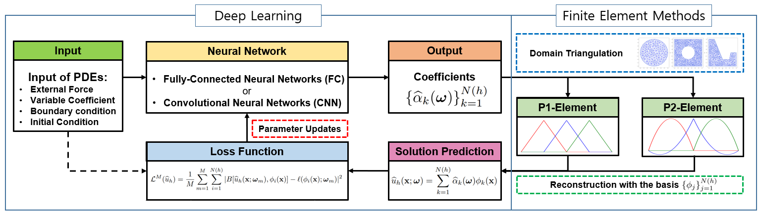
where is the FEM solution for the given PDEs. Motivated by (1), the FEONet can predict numerical solutions of the PDEs when given the initial conditions, external forcing functions, PDE coefficients, or boundary conditions as inputs. Therefore, the FEONet can learn multiple instances of the solutions of PDEs, making it a versatile approach for solving different types of PDEs in complex domains; see e.g. Figure 1. The loss function of the FEONet is designed based on the residual quantity of the finite element approximation, motivated by the classical FEM [11, 8]. This allows the FEONet to accurately approximate the solutions of PDEs, while also ensuring that the boundary conditions are exactly satisfied. This approach involves inferring coefficients, denoted as , which are subsequently utilized to construct the linear combination to approximate the solution of PDEs. Inheriting the capability of the FEM handling boundary conditions, the predicted solution will also satisfy the exact boundary condition. Additionally, since we have adopted the FEM as a baseline framework, we can expect that our proposed method is robust, reliable and accurate. It is noteworthy that due to the intrinsic structure of the proposed FEONet scheme, we do not need any paired input-output training data and hence the model can be trained in an unsupervised manner.
Another key contribution of this study is the introduction of a novel learning architecture designed to accurately solve convection-dominated singularly perturbed problems, which are characterized by strong boundary layer phenomena. These types of problems present significant challenges for traditional machine learning and numerical methods, primarily due to the sharp transitions within thin layers caused by a small diffusive parameter. In particular, this is challenging in the realm of learning theory, where neural networks typically assume a smooth prior, making them less equipped to handle such abrupt transitions effectively. By adapting theory-guided methods [10], the network effectively captures the behavior of boundary layers, an area that has been underexplored in recent machine-learning approaches.
The structure of this paper is outlined as follows: Section 2 provides a detailed elaboration on the proposed numerical scheme as well as the theoretical convergence results. Subsequently, Section 3 presents the experimental results, demonstrating the computational flexibility of FEONet in both 1D and 2D settings across various PDE problems. Finally, Section 4 summarizes this work.
2 Finite element operator network (FEONet)
In this section, we present our proposed method, the FEONet, by demonstrating how neural network techniques can be integrated into FEMs to solve the parametric PDEs. Throughout our method description and experiments, we focus on the PDEs of the following form: for uniformly elliptic coefficients and ,
| (2) |
Here can be either linear or nonlinear, and both cases will be covered in the experiments performed in Section 3. As will be described in more detail later, we shall propose an operator-learning-type method that can provide real-time solution predictions whenever the input data of the PDE changes.
In addition to the explanation for the proposed method, we will also describe the analytic framework of the FEONet, where we can discuss the convergence analysis of the method.
2.1 Model description
We begin with the following variational formulation of the given PDE (2): find satisfying
| (3) |
for a suitable function space . In the theory of FEM, the first step is to define a triangulation of the given domain , . We shall assume that is a collection of conforming shape-regular triangulations of , consisting of -dimensional simplices . The finite element parameter signifies the maximum mesh size of . In addition, let us denote by , the space of all continuous functions defined on such that the restriction of to an arbitrary triangle is a polynomial. Then we define our finite-dimensional ansatz space as . We shall denote the set of all vertices in the triangulation by , and define the nodal basis for , defined by .
Then the Galerkin approximation is as follows: find satisfying
| (4) |
If we write the finite element solution
| (5) |
the Galerkin approximation (4) is transformed into the linear algebraic system
| (6) |
where the matrix is invertible provided that the given PDEs have a suitable structure. Therefore, we can determine the coefficients by solving the system of linear equations (6), and consequently, produce the approximate solution as defined in (5).
Now, in this setting let us describe the method we propose in this paper. In our scheme, an input for the neural network is the data for the given PDEs. In this paper, we choose external force as a prototype input feature. Note, however, that the same scheme can also be developed with other types of data, e.g., boundary conditions, diffusion coefficients or initial conditions for time-dependent problems. See, for example, Section 3.2 where extensive experiments were performed addressing various types of input data. For this purpose, the external forcing terms are parametrized by the random parameter contained in the (possibly high-dimensional) parameter space . For each realization (and hence for each load vector defined in (6)), instead of computing the coefficients from the linear algebraic system (6), we approximate the coefficients by a deep neural network. More precisely, these input features representing external forces pass through the deep neural network and the coefficients are generated as an output of the neural network. We then reconstruct the solution
| (7) |
For the training, we use a residual of the variational formulation (4) and define the loss function by summing over all basis functions: for randomly chosen parameters ,
| (8) |
For each training epoch, once the neural network parameters are updated in the direction of minimizing the loss function (8), the external force passes through this updated neural network to generate more refined coefficients, and this procedure is repeated until the sufficiently small loss is achieved. A schematic diagram of the FEONet algorithm is depicted in Figure 2.
Remark 2.1.
To avoid confusion for readers, here we provide further clarification: in this paper, the term “training data” refers to the labeled data, specifically the pairs of pre-computed PDE data and their corresponding solutions. The term “input sample” is used to denote the randomly extracted points from the parametric domain. In this case, since they don’t require labeling, there is no computational cost associated with the sampling process. In summary, for the training of FEONet, only input samples are required and the model can be trained without the need for pre-computed training data.
2.2 Convergence analysis of FEONet
In this section, we address the convergence result of the FEONet which provides theoretical justification for the proposed method. As outlined in the previous subsection, the proposed method is based on the FEM, and the finite element approximation in (5) can be considered as an intermediate solution between the true solution of (3) and the approximate solution predicted by the FEONet.
For simplicity, we will focus on self-adjoint equations with homogeneous Dirichlet boundary conditions:
| (9) | ||||||
where the coefficient is uniformly elliptic and . In the present paper, we focus on the case when the finite element parameter is fixed and deal with the convergence of the FEONet prediction to the finite element solution . The analysis for general equations that cannot be covered by the form (9) and the theoretical analysis addressing the role of in the error estimate are of independent interest and will be investigated in the forthcoming paper.
Analytic framework
As described before, the input of neural networks is an external forcing term , which is parametrized by the random parameter in the probability space . In this section, we will regard as a bivariate function defined on , and assume that
| (10) |
for some constant . For each , the external force is determined, and the corresponding weak solution is denoted by which satisfies the following weak formulation:
| (11) |
For given , let be a conforming finite element space generated by the basis functions and be a finite element approximation of satisfying the Galerkin approximation
| (12) |
We shall write
| (13) |
where is the solution of the linear algebraic equations
| (14) |
with
| (15) |
In other words, in (13) is the finite element approximation of the solution to the equation (9), as described in Section 2.1. It is noteworthy that instead of the equations (14), can also be characterized in the following way:
| (16) |
where is the population loss
| (17) |
Next, we shall define a class of neural networks, that plays the role of an approximator for coefficients. For each , we write an -layer neural network by a function , defined by
| (18) |
where and are the weight and the bias respectively for the -th layer, and is a nonlinear activation function. We denote the architecture by the vector , the class of neural network parameters by , and its realization by . For a given neural network architecture , the family of all possible parameters is denoted by
| (19) |
For two neural networks , , with architectures , we write if for any , there exists satisfying for all .
Now let us assume that there exists a sequence of neural network architectures satisfying for all . We define the associated collection of neural networks by
| (20) |
It is straightforward to verify that for any . We start with the following theorem. This is known as the universal approximation theorem, and known to hold in various scenarios [13, 20, 42].
Theorem 2.2.
Let be a compact set in and assume that . Then there holds
| (21) |
In the present paper, the target function to be approximated by neural networks is . Due to the assumption (10), we can verify that is continuous and bounded. This motivates us to deal with the family of bounded neural networks as an ansatz space. For this, let us write , and assume that is a bounded activation function with continuous inverse (e.g., sigmoid or tanh activation functions) with and . We then define a function satisfying , . By the assumptions, also has a continuous inverse. With the above notations, we consider the following family of neural networks:
| (22) |
where we can see that
| (23) |
In the analysis, we will use the following version of the universal approximation theorem for bounded neural networks, which is quoted from [23].
Theorem 2.3.
Now, with the notation defined above, as a neural network approximation of , we seek for solving the residual minimization problem
| (25) |
where the loss function is minimized over , and we shall write the corresponding solution by
| (26) |
Note that for the neural network under consideration , the input vector is which determines the external force and the output is the coefficient vector in .
As a final step, let us define the solution to the following discrete residual minimization problem:
| (27) |
where is the empirical loss defined by the Monte–Carlo integration of :
| (28) |
with is an i.i.d. sequence of random variables distributed according to . Then we write the corresponding solution as
| (29) |
which is the numerical solution actually computed by the scheme proposed in the present paper. In this paper, we assume that it is possible to find the exact minimizers for the problems (25) and (27), and the error that occurred by the optimization can be ignored.
In order to provide appropriate theoretical backgrounds for the proposed method, it would be reasonable to show that our solution is sufficiently close to the approximate solution computed by the proposed scheme for various external forces, as the index for a neural-network architecture and the number of input samples goes to infinity. Mathematically, it can be formulated as
| (30) |
The main error can be split into three parts:
| (31) |
The first error is the one caused by the finite element approximation, which is assumed to be negligible for a proper choice of . In fact, according to the classical theory of the FEM (e.g. [8, 11]) if is sufficiently small, then we can expect to obtain a sufficiently small error. Therefore, in this paper, we shall assume that we have chosen suitable which guarantees a sufficiently small error for the finite element approximation and only focus on the convergence of with a fixed .
The second error is referred to as the approximation error, as it appears when we approximate the target function with a class of neural networks. The third error is often called the generalization error, which measures how well our approximation predicts solutions for unseen data. We will focus on proving that our approximate solution converges to the finite element solution (which is sufficiently close to the true solution) as a neural network architecture grows and the number of input samples goes to infinity, i.e., we will show that
Approximation error
We first note from (17) and (28), that defined in (13), (14) mostly determines the structures of the loss functions and it would be advantageous for us to analyze the loss function if we know more about the matrix. Note that the matrix is determined by the structure of the given differential equations, the choice of basis functions and the boundary conditions. Therefore, the characterization of which is useful for the analysis of the loss function and can cover a wide range of PDE settings simultaneously is important. The next lemma addresses this issue, which is quoted from [23].
Lemma 2.4.
Suppose that the matrix is symmetric and invertible, and let , where is the family of eigenvalues of the matrix . Then we have for all ,
| (32) |
Since the equation under consideration (9) is self-adjoint, the corresponding bilinear form defined in (11) is symmetric which automatically guarantees that the matrix in our case is symmetric. Furthermore, due to the facts that the coefficient is uniformly elliptic and is non-negative, the bilinear form is coercive, which implies that is positive-definite. Therefore, we can apply Lemma 2.4 to the matrix of our interest.
We are now ready to present our first convergence result regarding the approximation error. The proof is based on Lemma 2.4 and can be found in Appendix A.1.
Theorem 2.5.
Generalization error
In order to handle the generalization error, we first introduce the concept so-called Rademacher complexity [5].
Definition 2.6.
For a collection of i.i.d. random variables, we define the Rademacher complexity of the function class by
where ’s denote i.i.d. Bernoulli random variables, in other words, for all .
Note that the Rademacher complexity is the expectation of the maximum correlation between the random noise and the vector , where the supremum is taken over the class of functions . By intuition, the Rademacher complexity of is often used to measure how the functions from can fit random noise. For a more detailed discussion on the Rademacher complexity, see [18, 48, 45].
Now we define the function class of interest
| (34) |
where the matrix and the vector are defined in (15). In the following theorem, note that we assume that for any , the Rademacher complexity of converges to zero, which is known to be true in many cases [45, 14, 37]. For the proof of the theorem below, see Appendix A.2.
Theorem 2.7.
Convergence of FEONet
From Theorem 2.5 and Theorem 2.7 combined with the triangular inequality, we have probability 1 over i.i.d. samples that
| (35) |
Based on the convergence of the approximate coefficients (35), let us now state the convergence theorem for the predicted solution, whose proof is presented in Appendix A.3.
Theorem 2.8.
Suppose (10) holds, and assume that for all , as , with . Then for given , we have with probability over i.i.d. samples that
| (36) |
3 Numerical experiments
In this section, we demonstrate the experimental results of the FEONet across various settings for PDE problems. We randomly generate 3000 input samples for external forces and train the FEONet in an unsupervised manner without the usage of pre-computed input-output pairs. We then evaluate the performance of our model with another randomly generated test set consisting of 3000 pairs of and the corresponding solutions . For this test data, we employed the FEM with a sufficiently fine mesh discretization to ensure that the numerical solutions can be considered as true solutions (See Appendix B.1). While there are other operator-learning-based methods, such as PINO [30], that can be trained without input-output data pairs, they often face limitations when dealing with domains of complex shapes. Consequently, our primary comparison will be against the DeepONet [34], taking into account varying numbers of training data, and PIDeepONet [49]. The triangulation of domains and the generation of the nodal basis for the FEM are performed using FEniCS [2, 33]. A detailed description of the model used in the experiments can be found in Appendix B.
In Section 3.1, we will solve PDE problems in various environments and settings to verify the computational flexibility of our method. In Section 3.2, we will confirm the flexibility of the proposed operator learning method by employing various types of input functions, and in Section 3.3, we will demonstrate that the FEONet framework can make an accurate solution prediction for the singular perturbation problems. Finally, in Section 3.4, additional experiments will be conducted to confirm the robustness and reliability of our method across various performance metrics. Throughout the experiments, we will cover both one-dimensional and two-dimensional cases, and we have appropriately organized them according to the objectives of each experiment.
| Model (#Train data) | Domain I | Domain II | Domain III | BC I | BC II | Eq I | Eq II |
|---|---|---|---|---|---|---|---|
| DON (supervised, w/30) | 27.151.16 | 51.213.58 | 53.924.59 | 21.751.19 | 22.751.05 | 24.381.37 | 10.260.14 |
| DON (supervised, w/300) | 2.100.75 | 5.620.37 | 6.220.96 | 0.680.11 | 0.960.06 | 0.760.10 | 0.200.09 |
| DON (supervised, w/3000) | 0.690.17 | 4.750.75 | 6.201.00 | 0.530.36 | 0.330.09 | 0.330.27 | 0.240.13 |
| PIDeepONet (w/o labeled data) | 9.80 | 101.03167.46 | 32.89 | 1.51 | 1.43 | 19.41 | 2.66 |
| Ours (w/o labeled data) | 1.240.00 | 1.760.03 | 0.510.00 | 0.130.01 | 0.320.03 | 0.130.01 | 0.540.07 |
3.1 Performance evaluation in various scenarios
To evaluate the computational flexibility of the FEONet, we conducted a sequence of experiments covering diverse domains, boundary conditions, and equations.
Various domains
We consider the 2D convection-diffusion equation as
| (37) | ||||||
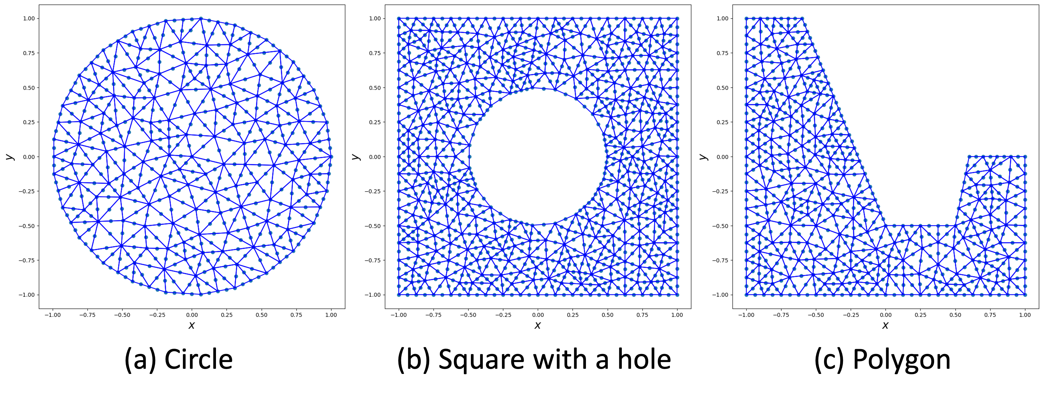
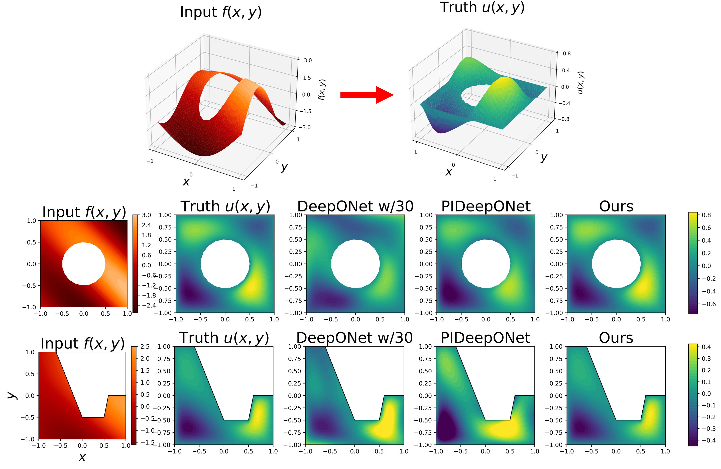
For our numerical experiments, we fixed the values of and across various domains , which included a circle, a square with a hole, and a polygon (see Figure 1). The second to fourth columns of Table 1 display the mean relative errors of the test set for FEONet (w/o labeled data), PIDeepONet (w/o labeled data), and DeepONet (with 30/300/3000 input-output data pairs) across various domains. When the DeepONet is trained with either 30 or 300 data pairs, FEONet consistently surpasses them in terms of numerical errors. Notably, even when DeepONet is trained with 3000 data pairs, FEONet achieves errors that are either comparable to or lower than those of DeepONet. It’s noteworthy that in more intricate domains like Domain II and Domain III, both the DeepONet (even with 3000 data pairs) and PIDeepONet find it challenging to produce accurate predictions. Figure 3 demonstrates the solution profile, emphasizing that FEONet is more precise in predicting the solution than both DeepONet and PIDeepONet, particularly in complex domains.
Various boundary conditions
We tested the performance of each model when the given PDEs were equipped with either Dirichlet or Neumann boundary conditions. We consider the convection-diffusion equation as
| (38) | ||||||
where and . For the Neumann boundary condition, we add to the left-hand side of (38) to address the uniqueness of the solution. The FEONet has an additional significant advantage to make the predicted solutions satisfy the exact boundary condition, by selecting the appropriate coefficients for the basis functions. Using the FEONet without any input-output training data, we are able to obtain similar or slightly higher accuracy compared to the DeepONet with 3000 training data, for both homogeneous Dirichlet or Neumann boundary conditions as shown in Table 1.
Various equations
We performed some additional experiments applying the FEONet to the various equations: (i) general second-order linear PDE with variable coefficients defined as
| (39) | ||||
where , and ; and (ii) the Burgers’ equation defined as
| (40) | ||||||
Since the Burgers’ equation is nonlinear, an iterative method is required for classical numerical schemes including the FEM, which usually causes some computational costs. Furthermore, it is more difficult than linear equations to obtain training data for nonlinear equations. One important advantage of the FEONet is its ability to effectively learn the nonlinear structure without any training data. Once the training process is completed, the model can provide accurate real-time solution predictions without relying on iterative schemes. The 7th and 8th columns of Table 1 highlight the effectiveness of the FEONet, predicting the solutions with reasonably low errors for various equations. Although the 8th column of Table 1 shows that the DeepONet with 3000 training data has a lower error compared to our model, it demonstrates the strength of the FEONet that achieves a similar level of accuracy even for the nonlinear PDE, that can be trained in an unsupervised manner.
3.2 Various types of input functions
In this section, we will demonstrate that our method can accommodate various types of input functions. Specifically, we shall utilize, as an input for our model, variable coefficients, boundary conditions and initial conditions for time-dependent problems. Furthermore, for the case of the vector-valued input functions, we will also include the solution prediction for the 2D Stokes problem. Throughout the series of experiments, we will confirm that our approach can make a fast and accurate solution prediction for such various scenarios.
Variable coefficient as an input
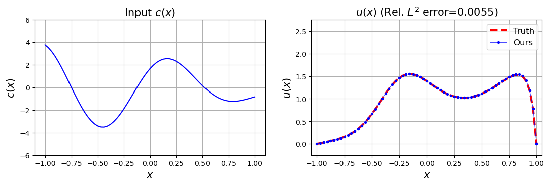
The FEONet is capable of learning the operator mapping from the variable coefficient to the corresponding solution of a PDE (39). Figure 4 displays the solution profile obtained when variable coefficients are considered as input. This highlights the flexibility of FEONet in adapting to a wide range of input function types, thereby underscoring its versatility.
Boundary condition as an input
We address the case when the input is a boundary condition. We consider the 2D Poisson equation as
| (41) | ||||||
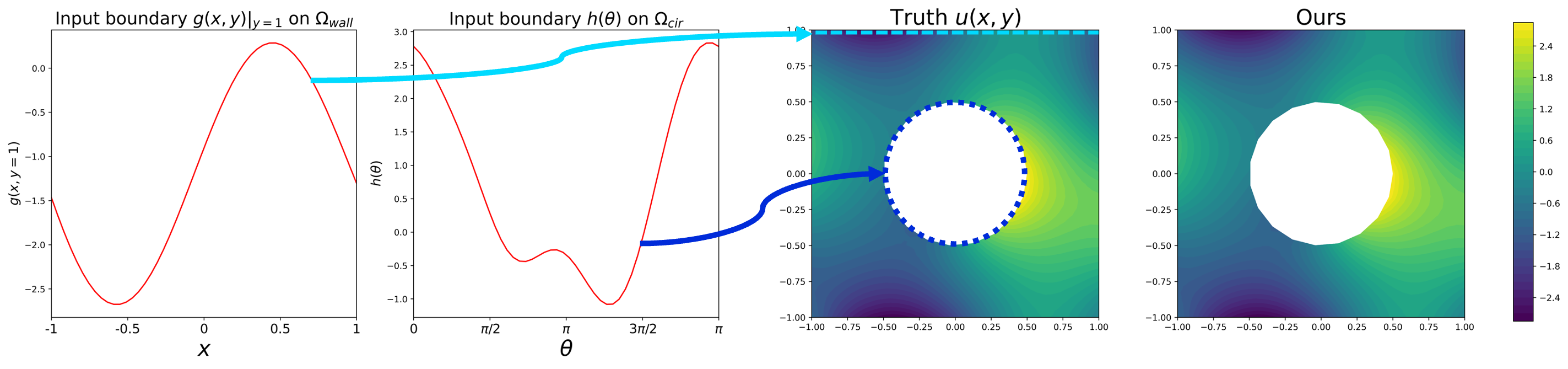
where and the domain is a square with a hole (see (b) in Figure 1). The FEONet is utilized to learn the operator . Figure 5 demonstrates that even in the case of an operator that takes the boundary condition as input, we can predict the solution with high accuracy. This demonstrates the versatility and adaptability of the FEONet approach for accommodating different types of input functions.
Initial condition as an input
The FEONet can be extended to handle the initial conditions as input. We consider the time-dependent problem with varying initial conditions. We consider the 1D convection-diffusion equation
| (42) | ||||||
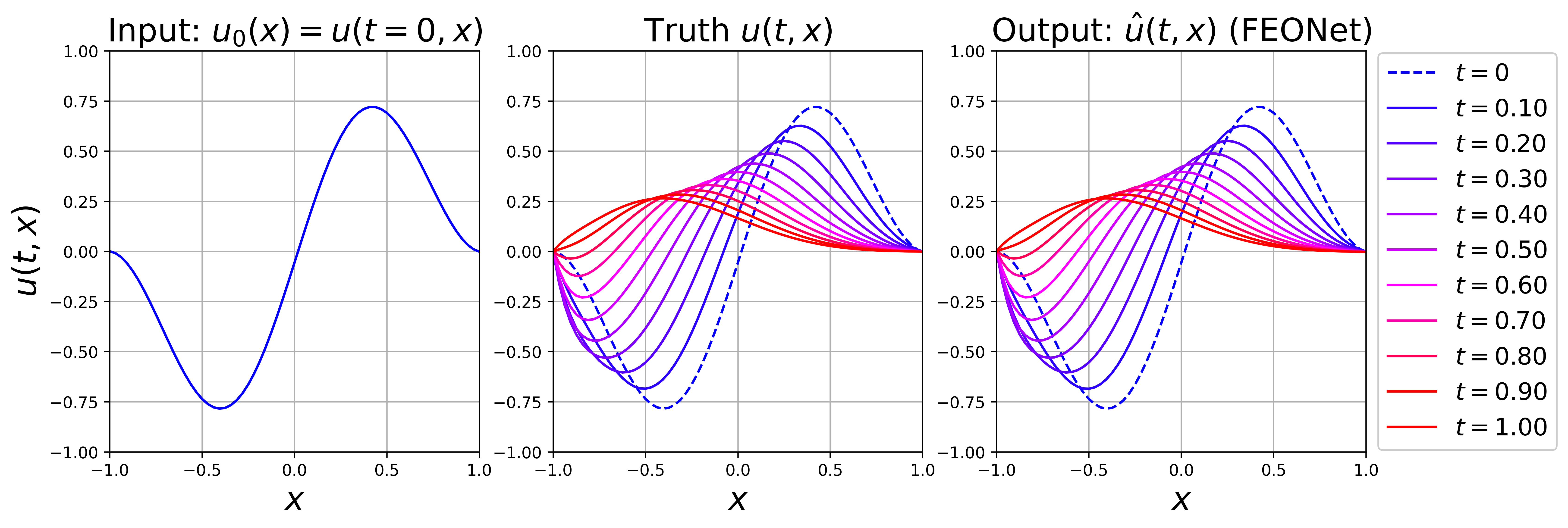
where and . We aim to learn the operator . We use the implicit Euler method to discretize the time with . We employed the marching-in-time scheme proposed by [24] to sequentially learn and predict solutions over the time domain , divided into 10 intervals. For training FEONet, we utilized only the input function and equation (42) without any additional data. Figure 6 illustrates FEONet’s effective prediction of true solutions using an initial condition from the test dataset.
Vector-valued function as an input: 2D Stokes equation
We consider a more intricate yet practical fluid dynamics issue: the two-dimensional steady-state Stokes equations, which can be described as follows:
| (43) | ||||||
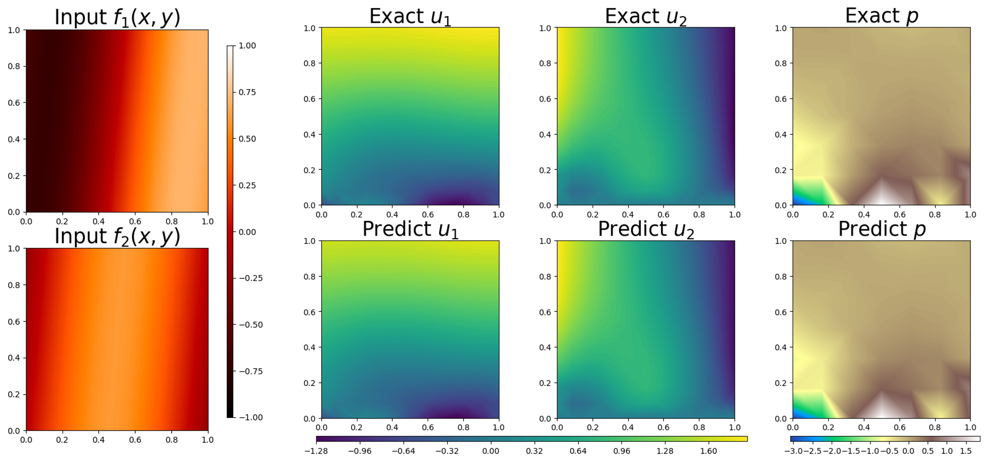
where . We aim to learn the operator using the FEONet. For this, we employ the P2 Lagrange element for velocity and the P1 Lagrange element for pressure. Together, this combination is known as the Taylor-Hood element [15]. Figure 7 demonstrates the results of the operator learning for the 2D Stokes equation using FEONet. This illustrates that FEONet is applicable to the learning of operators for the system of PDEs with vectorial inputs and outputs.
3.3 Singular perturbation problem
One of the notable advantages of the FEONet, which predicts coefficients through well-defined basis functions, is its applicability to problems involving singularly perturbed PDEs. The boundary layer problem is a well-established challenge in scientific computing. This issue arises from the presence of thin regions near boundaries where the solution exhibits steep gradients. Such regions significantly impact the overall behavior of the system. Typically, in cases where the target function demonstrates abrupt transitions, such as when the diffusion coefficient is small in our model problem, neural network algorithms frequently encounter difficulties in converging to optimal solutions. This is largely due to the phenomenon known as spectral bias [43]. Neural networks are generally predicated on a smooth prior assumption, but spectral bias leads to a failure to accurately capture abrupt transitions or singular behaviors of the target solution function. To address this challenge, we propose a novel semi-analytic machine learning approach, guided by singular perturbation analysis, for effectively capturing the behavior of thin boundary layer. This is accomplished by incorporating additional basis functions guided by theoretical considerations. For this we consider
| (44) | ||||||
where . For the implementation, we assign the values of and . For instance, in the right panel of Figure 8, the red dotted line (ground-truth) shows the solution profile which produces a sharp transition near . To capture the boundary layer, we utilize an additional basis function known as the corrector function in mathematical analysis, defined as
| (45) |
| Model | Ours | PINN | DeepONet w/30 | PIDeepONet |
|---|---|---|---|---|
| Requirement for labeled data | No | No | Yes | No |
| Multiple instance | Yes | No | Yes | Yes |
| Mean Rel. test errorstd | 0.01320.0091 | 1.38270.7580 | 0.23030.0074 | 0.57130.0007 |
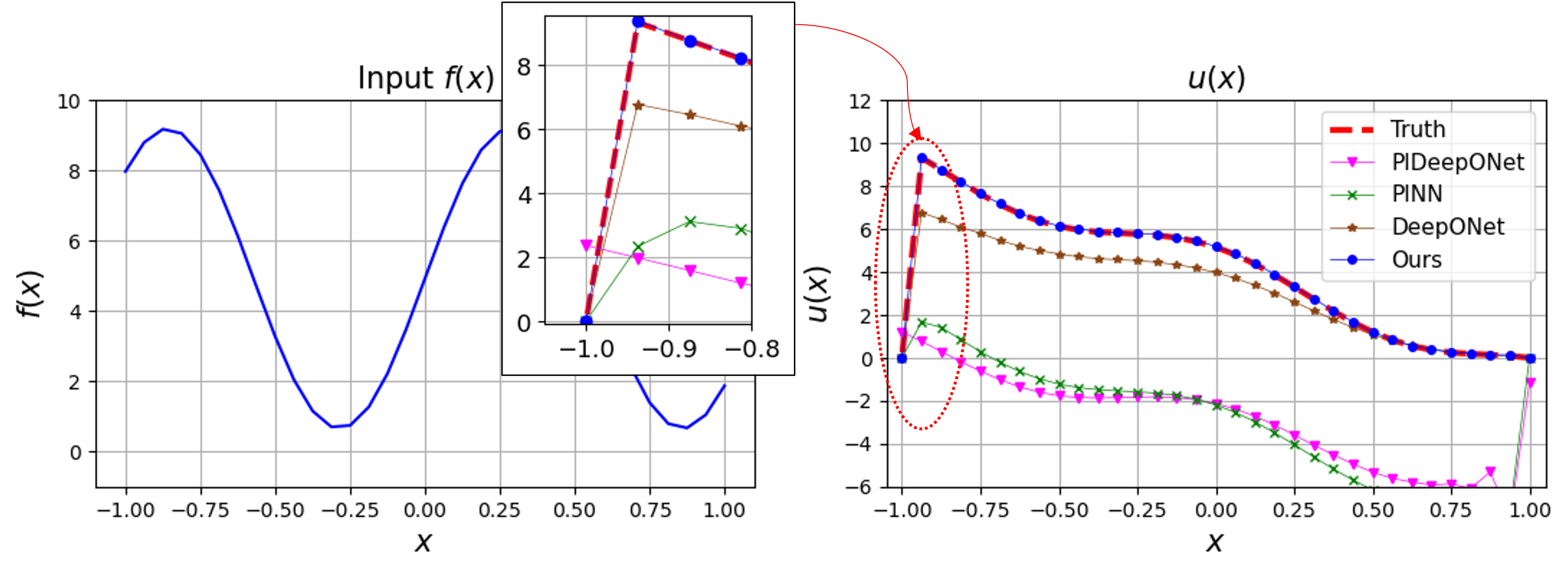
By integrating the boundary layer element into the finite element space, we establish the proposed enriched Galerkin space for utilization in the FEONet. As the corrector basis is incorporated alongside the conventional nodal basis functions in the FEM, we also predict the additional coefficient originating from the corrector basis. Note that the computational cost remains minimal as the enriched basis exclusively encompasses boundary elements. Table 2 summarizes the characteristics of various operator learning models and the corresponding errors when solving the singularly perturbed PDE described in (44). The performance of the FEONet in accurately solving boundary layer problems surpasses that of other models, even without labeled data, across multiple instances. The incorporation of a very small in the residual loss of the PDE makes operator learning challenging or unstable when using PINN and PIDeepONet. In fact, neural networks inherently possess a smooth prior, which can lead to difficulties in handling boundary layer problems. In contrast, FEONet utilizes theory-guided basis functions, enabling the predicted solution to accurately capture the sharp transition near the boundary layer. The PIDeepONet faces difficulties in effectively learning both the residual loss and boundary conditions, while PINNs struggle to predict the solution. Figure 8 exhibits the results of operator learning for the singular perturbation problem. As depicted in the zoomed-in graph of Figure 8, the FEONet stands out as the only model capable of accurately capturing sharp transitions, whereas other models exhibit noticeable errors.
3.4 Further performance metrics
Generalization errors
The FEONet is a model capable of learning the operator without the need for paired input-output training data. What we need for the training is the generation of random input samples, which only imposes negligible computational cost. Therefore, the number of input function samples for the FEONet training can be chosen arbitrarily. In the experiments performed in Section 3, we generated 3000 random input function samples to train the FEONet. On the other hand, the DeepONet requires paired input-output training data for supervised learning which causes significant computational costs to prepare. In this paper, we have focused our experiments on considering the DeepONet trained with 30, 300, and 3000 input-output data pairs. This allowed us to highlight the FEONet’s ability to achieve a certain level of accuracy without relying on data pairs.
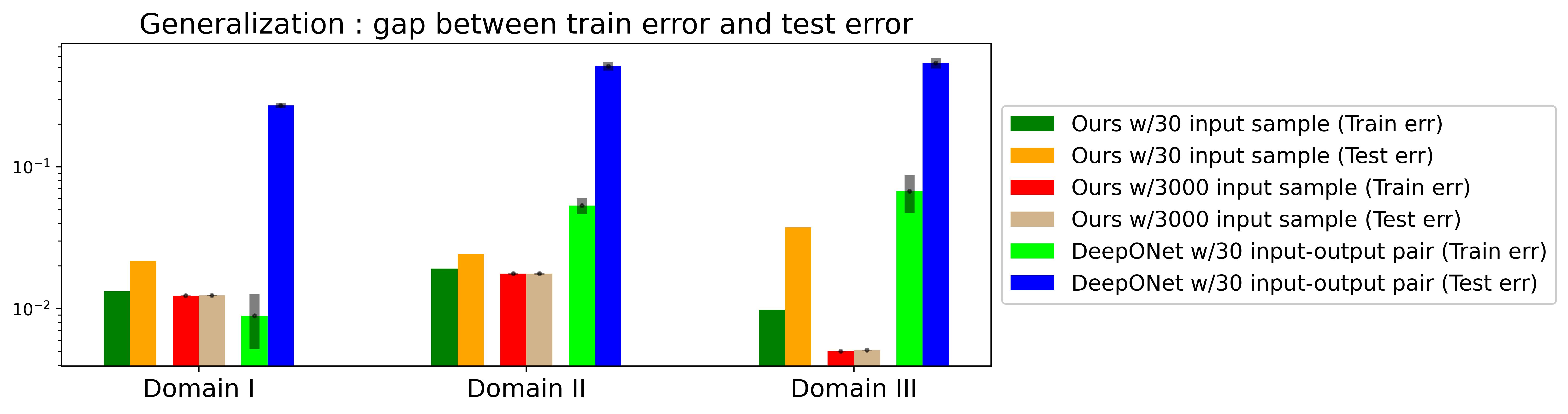
We present the results comparing generalization capability in Figure 9, when the FEONet is trained only with 30 random input samples (green and yellow bar) (which should be distinguished from 30 input-out data pair for the supervised learning). Figure 9 depicts a comparison of train and test errors between the FEONet, trained through an unsupervised approach with 30 and 3000 input samples, and the DeepONet, trained through supervised learning with 30 input-output data pairs. The disparity between the training error and the test error serves as a reliable indicator of how effectively the models generalize the underlying phenomenon. Notably, the FEONet shows superior generalization compared to the DeepONet, even without requiring input-output paired data. Remarkably, utilizing only 30 input samples for training, the FEONet achieves significantly better generalization and exhibits lower test errors than that of the DeepONet.
Rate of convergence
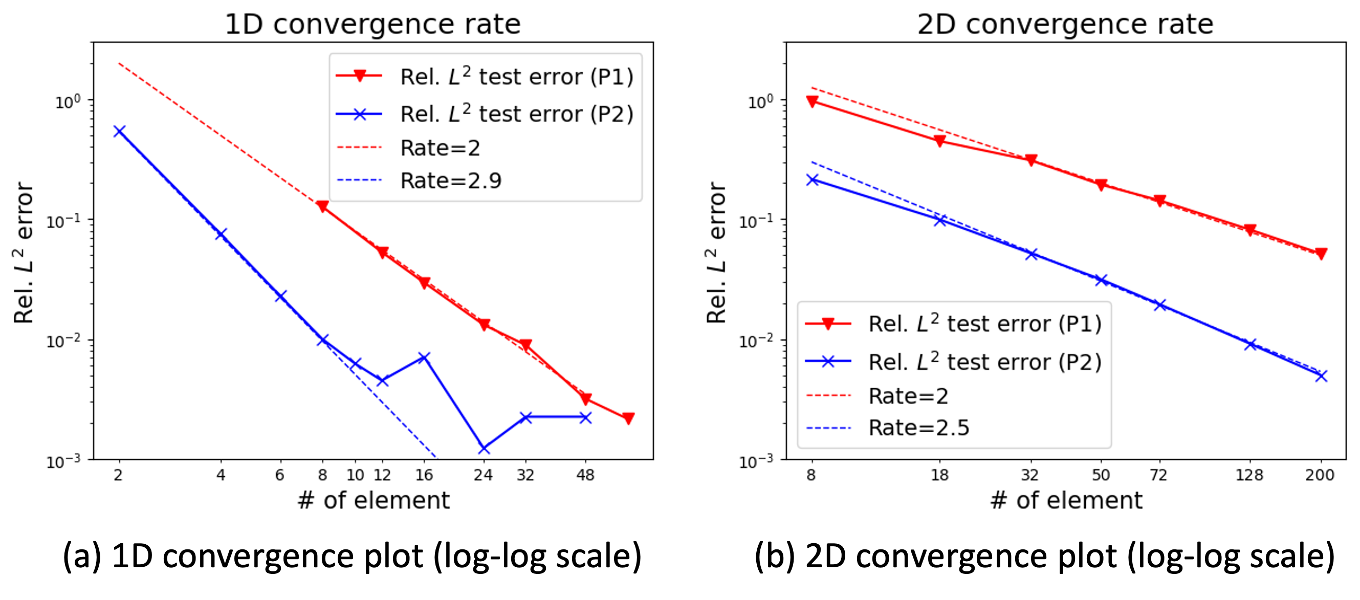
One of the intriguing aspects is that the theoretical results on the convergence error rate of the FEONet are also observable in the experimental results. Figure 10 shows the relationship between the test error and the number of elements, utilizing both P1 and P2 basis functions. In 1D problems, the convergence rate is approximately 2 for P1 basis functions and 2.9 for P2 basis functions. Meanwhile, in 2D problems, the convergence rate is approximately 2 for P1 basis functions and 2.5 for P2 basis functions. These remarkable trends confirm the theoretical convergence rates observed in the experimental results.
4 Conclusions
In this paper, we introduce the FEONet, a novel deep learning framework that approximates nonlinear operators in infinite-dimensional Banach spaces using finite element approximations. Our operator learning method for solving PDEs is both simple and remarkably effective, resulting in significant improvements in predictive accuracy, domain flexibility, and data efficiency compared to existing techniques. Furthermore, we demonstrate that the FEONet is capable of learning the solution operator of parametric PDEs, even in the absence of paired input-output training data, and accurately predicting solutions that exhibit singular behavior in thin boundary layers. The FEONet is capable of learning the operator by incorporating not only external forces but also boundary conditions, variable coefficients, and the initial conditions of time-dependent PDEs. We are confident that the FEONet can provide a new and promising approach to simulate and model intricate, nonlinear, and multiscale physical systems, with a wide range of potential applications in science and engineering.
Appendix A Proof of theoretical results
A.1 Approximation error
We shall prove Theorem addressing the approximation error for the coefficients.
Proof A.1 (Proof of Theorem 2.5).
Since is symmetric and invertible, by Proposition 2.4, we obtain
Note that the constants appearing in the inequalities above may depend on . But as we mentioned before, we assumed that is fixed with the sufficiently small finite element error. Then by the universal approximation property , as , which completes the proof.
A.2 Generalization error
Next, we shall find the connection between the generalization error and the Rademacher complexity for the uniformly bounded function class . In the following theorem, we assume that the function class is -uniformly bounded, meaning that for arbitrary .
Theorem A.2.
[Theorem 4.10 in [48]] Assume that the function class is -uniformly bounded and let . Then for arbitrary small , we have
with probability at least .
Next, note from Lemma 2.4 that
Since the class of neural networks under consideration is uniformly bounded and (10) holds, we see that for any , is -uniformly bounded for some . Then the following lemma is the direct consequence of Theorem A.2 within our setting.
Lemma A.3.
Let be i.i.d. random samples selected from the distribution . Then for arbitrary small , we obtain with probability at least that
| (46) |
Now from Lemma A.3, we shall prove Theorem concerning the generalization error for the coefficients.
Proof A.4 (Proof of Theorem 2.7).
A.3 Convergence of FEONet
Based on the results proved above, now we can address the convergence of the predicted solution by the FEONet to the finite element solution.
Appendix B Experimental details
B.1 Types and random generation of input functions for FEONet
In order to train the network, we generate random input functions (e.g. external forcing functions, variable coefficient functions, boundary conditions, and initial conditions). Inspired by [4], we created a random signal as a linear combination of sine functions and cosine functions. More precisely, we use
| (48) |
for a 1D case and
| (49) |
for a 2D case where for and for are drawn independently from the uniform distributions. In our experiments for DeepONet with input-output data pairs, we prepare a total of 30/300/3000 pairs of by applying the FEM on sufficiently fine meshes. It is worth noting that even when considering different random input functions, such as those generated by Gaussian random fields, we consistently observe similar results. This robustness indicates the reliability and stability of the FEONet approach across various input scenarios.
B.2 Plots on convergence rates
Let us make some further comments on the experimental details for Figure 10. For 1D case, we consider the convection-diffusion equation
| (50) | ||||||
where and . For the 2D case, we consider the following equation
| (51) | ||||||
where and . The FEONet was used to approximate the solution of these two equations using P1 and P2 nodal basis functions, and the experiments were conducted with varying domain triangulation to have different numbers of elements to observe the convergence rate. As shown in Figure 10, the observed convergence rate of the FEONet shows the convergence rates close to 2 and 3 for P1 and P2 approximation respectively, which are the theoretical results for the classical FEM. Since the precision scale of the neural network we used here is about , we cannot observe the exact trends in rates below this level of error. We expect to see the same trend even at lower errors if we use larger scale and more advanced models than the CNN structure.
B.3 Additional plot on generalization error
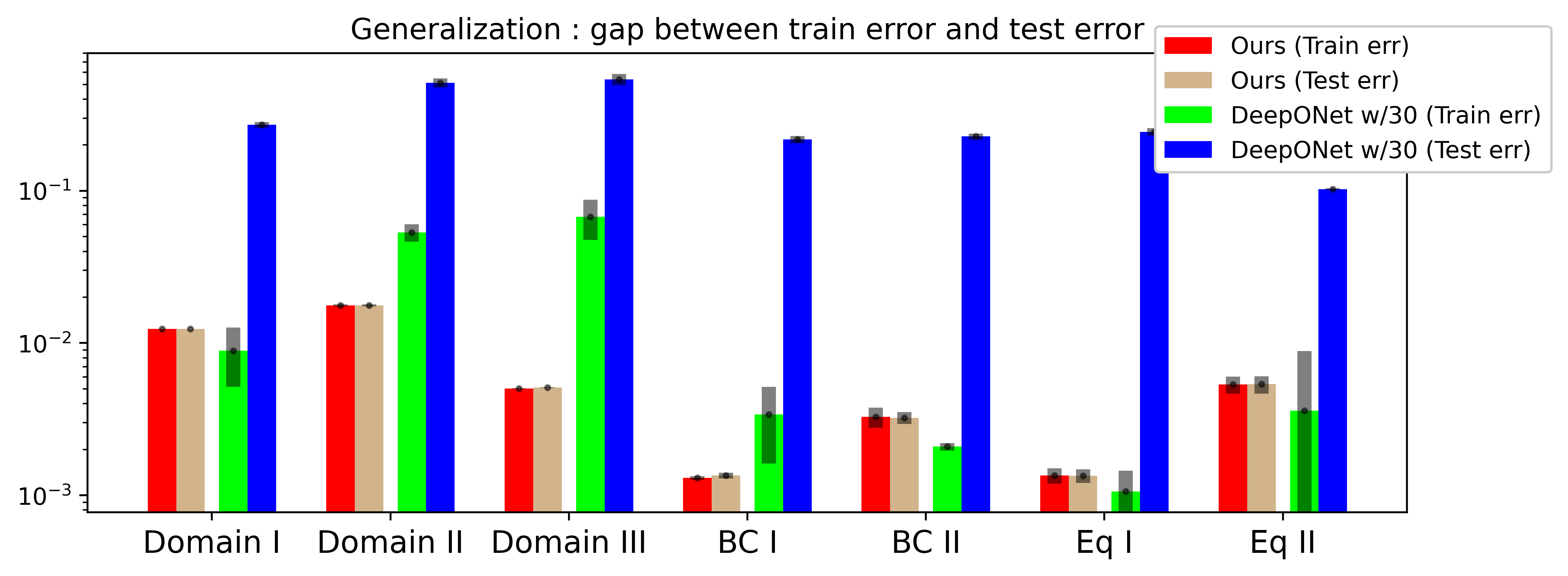
Figure 11 displays a comparison of the training and test errors between FEONet (w/o labeled data) and DeepONet (with 30 training data pairs) across different settings as performed in Section 3 (Table 1). We used 3000 input samples to train the FEONet and 30 input-output data pairs to train the DeepONet. Even with the 30 data pairs, there occurred a lot of computational costs to gain the data. Although it is predictable that increasing the number of input-output data pairs for the DeepONet would narrow the gap between train and test errors, preparing a large amount of data causes significant computational costs. As depicted in Figure 11, the generalization error of FEONet is notably smaller in comparison to that of DeepONet when trained with 30 data pairs.
References
- [1] M. Alber, A. Buganza Tepole, W. R. Cannon, S. De, S. Dura-Bernal, K. Garikipati, G. Karniadakis, W. W. Lytton, P. Perdikaris, L. Petzold, et al., Integrating machine learning and multiscale modeling—perspectives, challenges, and opportunities in the biological, biomedical, and behavioral sciences, NPJ digital medicine, 2 (2019), p. 115.
- [2] M. S. Alnaes, J. Blechta, J. Hake, A. Johansson, B. Kehlet, A. Logg, C. Richardson, J. Ring, M. E. Rognes, and G. N. Wells, The FEniCS project version 1.5, Archive of Numerical Software, 3 (2015), https://doi.org/10.11588/ans.2015.100.20553.
- [3] K. Atkinson, An introduction to numerical analysis, John wiley & sons, 1991.
- [4] Y. Bar-Sinai, S. Hoyer, J. Hickey, and M. P. Brenner, Learning data-driven discretizations for partial differential equations, Proceedings of the National Academy of Sciences, 116 (2019), pp. 15344–15349.
- [5] P. L. Bartlett and S. Mendelson, Rademacher and Gaussian complexities: risk bounds and structural results, J. Mach. Learn. Res., 3 (2002), pp. 463–482, https://doi.org/10.1162/153244303321897690, https://doi.org/10.1162/153244303321897690.
- [6] E. A. Bender, An introduction to mathematical modeling, Courier Corporation, 2000.
- [7] J. Brandstetter, D. E. Worrall, and M. Welling, Message Passing Neural PDE Solvers, in International Conference on Learning Representations, 2022, https://openreview.net/forum?id=vSix3HPYKSU.
- [8] S. C. Brenner and R. Scott, The Mathematical Theory of Finite Element Methods, Springer Science & Business Media, New York, 2008.
- [9] R. L. Burden, J. D. Faires, and A. M. Burden, Numerical analysis, Cengage learning, 2015.
- [10] M. D. Chekroun, Y. Hong, and R. Temam, Enriched numerical scheme for singularly perturbed barotropic quasi-geostrophic equations, Journal of Computational Physics, 416 (2020), p. 109493.
- [11] P. G. Ciarlet, The Finite Element Method for Elliptic Problems, Society for Industrial and Applied Mathematics, 2002, https://doi.org/10.1137/1.9780898719208, https://epubs.siam.org/doi/abs/10.1137/1.9780898719208, https://arxiv.org/abs/https://epubs.siam.org/doi/pdf/10.1137/1.9780898719208.
- [12] R. Courant and D. Hilbert, Methods of Mathematical Physics, Interscience, New York, 2nd ed., 1953. Translated from German: Methoden der mathematischen Physik I, 2nd ed, 1931 [15].
- [13] G. Cybenko, Approximation by superpositions of a sigmoidal function, Math. Control Signals Systems, 2 (1989), pp. 303–314, https://doi.org/10.1007/BF02551274, https://doi.org/10.1007/BF02551274.
- [14] W. E, C. Ma, and L. Wu, The Barron space and the flow-induced function spaces for neural network models, Constr. Approx., 55 (2022), pp. 369–406, https://doi.org/10.1007/s00365-021-09549-y, https://doi.org/10.1007/s00365-021-09549-y.
- [15] H. C. Elman, D. J. Silvester, and A. J. Wathen, Finite elements and fast iterative solvers: with applications in incompressible fluid dynamics, Oxford university press, 2014.
- [16] V. Fanaskov and I. Oseledets, Spectral Neural Operators, arXiv preprint arXiv:2205.10573, (2022).
- [17] N. A. Gershenfeld and N. Gershenfeld, The nature of mathematical modeling, Cambridge university press, 1999.
- [18] G. Gnecco and M. Sanguineti, Approximation error bounds via Rademacher’s complexity, Appl. Math. Sci. (Ruse), 2 (2008), pp. 153–176.
- [19] S. Goswami, M. Yin, Y. Yu, and G. E. Karniadakis, A physics-informed variational DeepONet for predicting crack path in quasi-brittle materials, Computer Methods in Applied Mechanics and Engineering, 391 (2022), p. 114587, https://doi.org/https://doi.org/10.1016/j.cma.2022.114587, https://www.sciencedirect.com/science/article/pii/S004578252200010X.
- [20] K. Hornik, Approximation capabilities of multilayer feedforward networks, Neural Networks, 4 (1991), pp. 251–257, https://doi.org/https://doi.org/10.1016/0893-6080(91)90009-T, https://www.sciencedirect.com/science/article/pii/089360809190009T.
- [21] T. J. R. Hughes, The Finite Element Method: Linear Static and Dynamic Finite Element Analysis, Dover Publications, 2000.
- [22] G. E. Karniadakis, I. G. Kevrekidis, L. Lu, P. Perdikaris, S. Wang, and L. Yang, Physics-informed machine learning, Nature Reviews Physics, 3 (2021), pp. 422–440.
- [23] S. Ko, S.-B. Yun, and Y. Hong, Convergence analysis of unsupervised Legendre-Galerkin neural networks for linear second-order elliptic PDEs, 2022, https://arxiv.org/abs/2211.08900.
- [24] A. Krishnapriyan, A. Gholami, S. Zhe, R. Kirby, and M. W. Mahoney, Characterizing possible failure modes in physics-informed neural networks, Advances in Neural Information Processing Systems, 34 (2021), pp. 26548–26560.
- [25] I. E. Lagaris, A. Likas, and D. I. Fotiadis, Artificial neural networks for solving ordinary and partial differential equations, IEEE transactions on neural networks, 9 (1998), pp. 987–1000.
- [26] M. G. Larson and F. Bengzon, The finite element method: theory, implementation, and applications, vol. 10, Springer Science & Business Media, 2013.
- [27] J. Y. Lee, S. CHO, and H. J. Hwang, HyperDeepONet: learning operator with complex target function space using the limited resources via hypernetwork, in The Eleventh International Conference on Learning Representations, 2023, https://openreview.net/forum?id=OAw6V3ZAhSd.
- [28] R. J. LeVeque, Finite-Volume Methods for Hyperbolic Problems, Cambridge University Press, 2002.
- [29] Z. Li, N. B. Kovachki, K. Azizzadenesheli, B. liu, K. Bhattacharya, A. Stuart, and A. Anandkumar, Fourier Neural Operator for Parametric Partial Differential Equations, in International Conference on Learning Representations, 2021, https://openreview.net/forum?id=c8P9NQVtmnO.
- [30] Z. Li, H. Zheng, N. B. Kovachki, D. Jin, H. Chen, B. Liu, K. Azizzadenesheli, and A. Anandkumar, Physics-informed neural operator for learning partial differential equations, CoRR, abs/2111.03794 (2021), https://arxiv.org/abs/2111.03794, https://arxiv.org/abs/2111.03794.
- [31] M. Lienen and S. Günnemann, Learning the Dynamics of Physical Systems from Sparse Observations with Finite Element Networks, in International Conference on Learning Representations, 2022, https://openreview.net/forum?id=HFmAukZ-k-2.
- [32] C.-C. Lin and L. A. Segel, Mathematics applied to deterministic problems in the natural sciences, SIAM, 1988.
- [33] A. Logg, K. Mardal, G. N. Wells, et al., Automated Solution of Differential Equations by the Finite Element Method, Springer, 2012, https://doi.org/10.1007/978-3-642-23099-8.
- [34] L. Lu, P. Jin, G. Pang, Z. Zhang, and G. E. Karniadakis, Learning nonlinear operators via DeepONet based on the universal approximation theorem of operators, Nature Machine Intelligence, 3 (2021), pp. 218–229.
- [35] L. Lu, X. Meng, S. Cai, Z. Mao, S. Goswami, Z. Zhang, and G. E. Karniadakis, A comprehensive and fair comparison of two neural operators (with practical extensions) based on fair data, Computer Methods in Applied Mechanics and Engineering, 393 (2022), p. 114778.
- [36] L. Lu, X. Meng, Z. Mao, and G. E. Karniadakis, DeepXDE: A deep learning library for solving differential equations, SIAM Review, 63 (2021), pp. 208–228.
- [37] Y. Lu, J. Lu, and M. Wang, A priori generalization analysis of the deep ritz method for solving high dimensional elliptic partial differential equations, in Proceedings of Thirty Fourth Conference on Learning Theory, M. Belkin and S. Kpotufe, eds., vol. 134 of Proceedings of Machine Learning Research, PMLR, 15–19 Aug 2021, pp. 3196–3241, https://proceedings.mlr.press/v134/lu21a.html.
- [38] X. Meng, Z. Li, D. Zhang, and G. E. Karniadakis, PPINN: Parareal physics-informed neural network for time-dependent PDEs, Computer Methods in Applied Mechanics and Engineering, 370 (2020), p. 113250.
- [39] S. T. Miller, N. V. Roberts, S. D. Bond, and E. C. Cyr, Neural-network based collision operators for the boltzmann equation, Journal of Computational Physics, 470 (2022), p. 111541.
- [40] M. E. Mortenson, Mathematics for computer graphics applications, Industrial Press Inc., 1999.
- [41] R. G. Patel, N. A. Trask, M. A. Wood, and E. C. Cyr, A physics-informed operator regression framework for extracting data-driven continuum models, Computer Methods in Applied Mechanics and Engineering, 373 (2021), p. 113500.
- [42] A. Pinkus, Approximation theory of the MLP model in neural networks, in Acta numerica, 1999, vol. 8 of Acta Numer., Cambridge Univ. Press, Cambridge, 1999, pp. 143–195, https://doi.org/10.1017/S0962492900002919, https://doi.org/10.1017/S0962492900002919.
- [43] N. Rahaman, A. Baratin, D. Arpit, F. Draxler, M. Lin, F. Hamprecht, Y. Bengio, and A. Courville, On the spectral bias of neural networks, in International Conference on Machine Learning, PMLR, 2019, pp. 5301–5310.
- [44] M. Raissi, P. Perdikaris, and G. E. Karniadakis, Physics-informed neural networks: A deep learning framework for solving forward and inverse problems involving nonlinear partial differential equations, Journal of Computational physics, 378 (2019), pp. 686–707.
- [45] S. Shalev-Shwartz and S. Ben-David, Understanding Machine Learning - From Theory to Algorithms., Cambridge University Press, 2014.
- [46] C. P. Simon, L. Blume, et al., Mathematics for economists, vol. 7, Norton New York, 1994.
- [47] J. C. Strikwerda, Finite difference schemes and partial differential equations, SIAM, 2004.
- [48] M. J. Wainwright, High-dimensional statistics, vol. 48 of Cambridge Series in Statistical and Probabilistic Mathematics, Cambridge University Press, Cambridge, 2019, https://doi.org/10.1017/9781108627771, https://doi.org/10.1017/9781108627771. A non-asymptotic viewpoint.
- [49] S. Wang, H. Wang, and P. Perdikaris, Learning the solution operator of parametric partial differential equations with physics-informed DeepONets, Science Advances, 7 (2021), p. eabi8605.
- [50] L. Yang, X. Meng, and G. E. Karniadakis, B-PINNs: Bayesian physics-informed neural networks for forward and inverse PDE problems with noisy data, Journal of Computational Physics, 425 (2021), p. 109913.
- [51] O. C. Zienkiewicz and R. L. Taylor, The Finite Element Method: Its Basis and Fundamentals, Butterworth-Heinemann, 2000.