This paper was converted on www.awesomepapers.org from LaTeX by an anonymous user.
Want to know more? Visit the Converter page.

Finite element method with the total stress variable for Biot’s consolidation model

Wenya Qi School of Mathematics and Statistics, Lanzhou University, Lanzhou 730000, China([email protected]). The research of W.Q. was partially supported by China Scholarship Council, Grant Number: 201906180039 and National Natural Science Foundation of China (Grant No.11471150).    Padmanabhan Seshaiyer Department of Mathematical Sciences, George Mason University, Fairfax, VA 22030, USA ([email protected]).    Junping Wang Division of Mathematical Sciences, National Science Foundation, Alexandria, VA 22314, USA([email protected]), and Department of Mathematical Sciences, George Mason University, Fairfax, VA 22030, USA. The research of J.W. was supported by the NSF IR/D program, while working at National Science Foundation. However, any opinion, finding, and conclusions or recommendations expressed in this material are those of the author and do not necessarily reflect the views of the National Science Foundation.
Abstract

In this work, semi-discrete and fully-discrete error estimates are derived for the Biot’s consolidation model described using a three-field finite element formulation. The fields include displacements, total stress and pressure. The model is implemented using a backward Euler discretization in time for the fully-discrete scheme and validated for benchmark examples. Computational experiments presented verifies the convergence orders for the lowest order finite elements with discontinuous and continuous finite element appropriation for the total stress.

keywords:
Biot’s consolidation model, the total stress, error estimate, fully-discrete, lowest finite elements.
AMS:
Primary 65N30; Secondary 65N50

1 Introduction

Biot’s fundamental equations for the soil consolidation process that describes the gradual adaptation of the soil to a load variation have been established in [1]. The mechanism of consolidation phenomenon described using a linear isotropic model is identical with the process of squeezing water out of an elastic porous medium in many cases. This solid-fluid coupling was extended to general anisotropy case in [2]. Such poroelasticity models have a lot applications in many areas including geomechanics [3], medicine [4], biomechanics [5], reservoir engineering [6]. The Biot’s consolidation models have also been used to combine transvascular and interstitial fluid movement with the mechanics of soft tissue in [7], which can be applied to improve drug delivery in solid tumors. Existence, uniqueness, and regularity theory were developed in [8] for poroelasticity and quasi-static problem in thermoelasticity. In [9], experiments with finite element method for the model in [7] have demonstrated the effects of fluid flow on the spatio-temporal patterns of soft-tissue elastic strain under a variety of physiological condition, which emphasized simulations relevant to a quasistatic elasticity imaging for the characterization of fluid flow in solid tumors.

Biot’s consolidation model has been considered by many researchers using finite element methods. In [10], a variational principle and the finite element method for a model with applications to a nonhomogeneous, anisotropic soil were developed. The fully discretization with backward Euler time discrete finite element method has been carried out and the existence and uniqueness were proved in [11]. Moreover, the simplest Taylor-Hood finite elements were employed. The stability and error estimates for the semi-discrete and fully-discrete finite element approximations were derived in [12] and [13]. Decay functions and post processing technique also were employed to improve the pore pressure accuracy. With the displacement and pore pressure fields as unknowns, the short and long time behavior of spatially discrete finite element solutions have been studied in [14]. Asymptotic error estimates have been derived for both stable and unstable combinations of the finite element spaces. For the coupled problem, a least squares mixed finite element method was presented and analyzed in [15] with the unknowns fluid displacement, stress tensor, flux, and pressure. In [16], coupling of mixed and continuous Galerkin finite element methods for pressure and displacements have been formulated deriving the convergence error estimates in time continuous setting. Methods for coupling mixed and discontinuous Galerkin have been presented in [17]. The error estimates for a fully-discrete stabilized discontinuous Galerkin method were obtained with the unknowns pressure and displacement in [18]. In [19], a discretization method in irregular domains with general grids for discontinuous full tensor permeabilities was developed. A new mixed finite element method for Biot’s consolidation problem in four variables was proposed in [20] and later, a three field mixed finite element which was free of pressure oscillations and Poisson locking has been proposed [21]. The priori error estimates that were robust for material parameters were provided in [22] with a four-field mixed method formulation. A three field finite element formulation with nonconforming finite element space for the displacements was considered in [23]. Based on the parameter dependent norms, the parameter-robust stability was established in [24], and parameter robust inf-sup stability and strong mass conservation were derived for three field mixed discontinuous Galerkin discretizations. A stabilized finite element method with equal order elements for the unknowns pressure and displacement was proposed in [25] to reduce the effects of non-physical oscillations. Combining the mixed method with symmetric interior penalty discontinuous Galerkin method obtained a H(div) conforming finite element method in [26]. The method achieved strong mass conservation.

Moreover, in [27], the total stress (or the soil pressure) expressed as a combination of the divergence of the velocity and pressure has been introduced coupling the solid and fluid robustly for Biot’s consolidation problem with the unknown displacement, pressure, and volumetric stress. Using a Fredholm argument for a static model, error estimates were derived independently of the Lame´\acute{e} constants for both continuous and discrete formulations. A three field formulation of Biot’s model with the total stress variable has also been proposed in [28], which developed a parameter-robust block diagonal preconditioner for the associated discrete systems. Then, in [29], a priori error estimates for semi-discrete scheme has been presented by introducing the total pressure variable for quasi-static multiple-network poroelasticity equations. Our goal in this paper is to emphasize the time dependence of field variables in error estimates, so we choose to consider the fully-discrete scheme. Thus, using the total stress as a new variable for the three field formulation, we give the error estimates for semi-discrete and fully-discrete with backward Euler time discretization schemes.

Let Ω\Omega be an open bounded polygonal or polyhedral domain in d,d=2,3\mathbb{R}^{d},~{}d=2,3. Biot’s consolidation model is described as follows: Find the displacement vector 𝐮\mathbf{u} and the fluid pressure pp in

(1) (2με(𝐮)+λ𝐮𝐈p𝐈)\displaystyle-\nabla\cdot(2\mu\varepsilon(\mathbf{u})+\lambda\nabla\cdot\mathbf{u}\mathbf{I}-p\mathbf{I}) =𝐟,inΩ×(0,T¯],\displaystyle=\mathbf{f},~{}~{}~{}~{}~{}~{}~{}~{}~{}~{}\mbox{in}~{}\Omega\times(0,\bar{T}],
(2) (Dt𝐮)(kp)\displaystyle\nabla\cdot(D_{t}\mathbf{u})-\nabla\cdot(k\nabla p) =g,inΩ×(0,T¯],\displaystyle=g,~{}~{}~{}~{}~{}~{}~{}~{}~{}~{}\mbox{in}~{}\Omega\times(0,\bar{T}],
(3) 𝐮=𝟎,p\displaystyle\mathbf{u}=\mathbf{0},~{}~{}p =0,onΓD×(0,T¯],\displaystyle=0,~{}~{}~{}~{}~{}~{}~{}~{}~{}~{}\mbox{on}~{}\Gamma_{D}\times(0,\bar{T}],
(4) (2με(𝐮)+λ𝐮𝐈p𝐈)𝐧\displaystyle(2\mu\varepsilon(\mathbf{u})+\lambda\nabla\cdot\mathbf{u}\mathbf{I}-p\mathbf{I})\cdot\mathbf{n} =β,onΓN×(0,T¯],\displaystyle=\mathbf{\beta},~{}~{}~{}~{}~{}~{}~{}~{}~{}~{}\mbox{on}~{}\Gamma_{N}\times(0,\bar{T}],
(5) (κp)𝐧\displaystyle(\kappa\nabla p)\cdot\mathbf{n} =γ,onΓN×(0,T¯],\displaystyle=\mathbf{\gamma},~{}~{}~{}~{}~{}~{}~{}~{}~{}~{}\mbox{on}~{}\Gamma_{N}\times(0,\bar{T}],

where ΓD\Gamma_{D} and ΓN\Gamma_{N} are disjoint closed subsets with ΓDΓN=Ω\Gamma_{D}\cup\Gamma_{N}=\partial\Omega and the Dirichlet boundary |ΓD|0|\Gamma_{D}|\neq 0. Here, ε(𝐮)=12(𝐮+(𝐮)T)\varepsilon(\mathbf{u})=\frac{1}{2}(\nabla\mathbf{u}+(\nabla\mathbf{u})^{T}) is the strain tensor expressed in terms of symmetrized gradient of displacements, κ(0,)\kappa\in(0,\infty) is the permeability of the porous solid and parameters μ(0,)\mu\in(0,\infty), λ(0,)\lambda\in(0,\infty) are the elastic Lame´\acute{e} constants. The right hand side term 𝐟\mathbf{f} in (1) represents the density of the applied body forces, and the source term gg in (2) represents a forced fluid extraction or injection. The outward unit normal vector on Ω\partial\Omega is denoted by 𝐧\mathbf{n}.

Next, we introduce the coupling between the solid and fluid using q=λ𝐮+pq=-\lambda\nabla\cdot\mathbf{u}+p, where qq is the total stress, 𝐮\mathbf{u} is the displacement and pp is the fluid pressure [27, 28]. This can be rewritten as

(6) λ1(qp)+𝐮=0.\lambda^{-1}(q-p)+\nabla\cdot\mathbf{u}=0.

For xΩx\in\Omega, the initial conditions are given by

(7) 𝐮(x,0)\displaystyle\mathbf{u}(x,0) =φ,\displaystyle=\varphi,
p(x,0)\displaystyle p(x,0) =ϕ.\displaystyle=\phi.

Hence, the initial condition for the total stress is q(x,0)=λφ+ϕq(x,0)=-\lambda\nabla\cdot\mathbf{\varphi}+\phi. Denote the spaces [H0,D1(Ω)]d={𝐯[H1(Ω)]d,𝐯=𝟎onΓD}[H^{1}_{0,D}(\Omega)]^{d}=\{\mathbf{v}\in[H^{1}(\Omega)]^{d},~{}\mathbf{v}=\mathbf{0}~{}\mbox{on}~{}\Gamma_{D}\} and H0,D1(Ω)={vH1(Ω),v=0onΓD}H^{1}_{0,D}(\Omega)=\{v\in H^{1}(\Omega),~{}v=0~{}\mbox{on}~{}\Gamma_{D}\}.

Multiplying (1), (6) and (2) by test functions, integrating by parts and applying boundary conditions yield the following weak formulation: Find 𝐮[H0,D1(Ω)]d\mathbf{u}\in[H^{1}_{0,D}(\Omega)]^{d}, qL2(Ω)q\in L^{2}(\Omega), pH0,D1(Ω)p\in H^{1}_{0,D}(\Omega) such that

(8) 2μ(ε(𝐮),ε(𝐯))(q,𝐯)\displaystyle 2\mu(\varepsilon(\mathbf{u}),\varepsilon(\mathbf{v}))-(q,\nabla\cdot\mathbf{v}) =(𝐟,𝐯)+β,𝐯ΓN,𝐯[H0,D1(Ω)]d,\displaystyle=(\mathbf{f},\mathbf{v})+\langle\beta,\mathbf{v}\rangle_{\Gamma_{N}},~{}~{}~{}~{}~{}~{}\forall\mathbf{v}\in[H^{1}_{0,D}(\Omega)]^{d},
(λ1(qp),wq)+(𝐮,wq)\displaystyle(\lambda^{-1}(q-p),w_{q})+(\nabla\cdot\mathbf{u},w_{q}) =0,wqL2(Ω),\displaystyle=0,~{}~{}~{}~{}~{}~{}~{}~{}~{}~{}~{}~{}~{}~{}~{}~{}~{}~{}~{}~{}~{}~{}~{}~{}~{}\forall w_{q}\in L^{2}(\Omega),
(λ1(qtpt),wp)+κ(p,wp)\displaystyle-(\lambda^{-1}(q_{t}-p_{t}),w_{p})+\kappa(\nabla p,\nabla w_{p}) =(g,wp)+γ,wpΓN,wpH0,D1(Ω).\displaystyle=(g,w_{p})+\langle\gamma,w_{p}\rangle_{\Gamma_{N}},~{}~{}\forall w_{p}\in H^{1}_{0,D}(\Omega).

In Section 2, we present the semi-discrete and fully-discrete finite element formulation for system (8) with the unknown displacement, total stress and pressure and prove uniqueness of the solution for each of these schemes. Section 3 presents the derivation and analysis of the error estimates for both the semi-discrete and fully-discrete schemes. In Section 4 we present computational experiments on benchmark problems that validate the theoretical convergence rates with respect to mesh size hh and time step τ\tau.

In the paper, we denote the arbitrary constants by ϵi0\epsilon_{i}\geq 0, where ii is positive integer and CC is a constant which is independent of time step τ\tau and mesh size hh. Let Pk{P}_{k} be the space of polynomials of degree less than or equal to kk in all variables. Moreover, let \|\cdot\| be the norm in L2(Ω)L^{2}(\Omega) space and k\|\cdot\|_{k} be the norm in Hk(Ω)H^{k}(\Omega) space. Denote the space-time space by Lk(0,T¯;V)L^{k}(0,\bar{T};V) for a Banach space VV (see details in [34]).

2 Finite Element Discretization and Uniqueness

Let 𝒯h\mathcal{T}_{h} be a regular and quasi-uniform triangulation of domain Ω\Omega into triangular or tetrahedron elements [30, 31]. For each element T𝒯hT\in\mathcal{T}_{h}, hTh_{T} is its diameter and h=maxT𝒯hhTh=\max_{T\in\mathcal{T}_{h}}h_{T} is the mesh size of triangulation 𝒯h\mathcal{T}_{h}. We consider the following finite element spaces on 𝒯h\mathcal{T}_{h},

𝐔h:=\displaystyle\mathbf{U}_{h}:= {𝐯[H0,D1(Ω)]d[C0(Ω)]d:𝐯T[Pk(T)]d,T𝒯h},\displaystyle\{\mathbf{v}\in[H^{1}_{0,D}(\Omega)]^{d}\cap[C^{0}(\Omega)]^{d}:\mathbf{v}\mid_{T}\in[{P}_{k}(T)]^{d},\forall T\in\mathcal{T}_{h}\},
Zh:=\displaystyle Z_{h}:= {qL2(Ω):qTPl(T),T𝒯h},\displaystyle\{q\in L^{2}(\Omega):q\mid_{T}\in{P}_{l}(T),\forall T\in\mathcal{T}_{h}\},
Ph:=\displaystyle P_{h}:= {pH0,D1(Ω)C0(Ω):pTPk1(T),T𝒯h},\displaystyle\{p\in H^{1}_{0,D}(\Omega)\cap C^{0}(\Omega):p\mid_{T}\in{P}_{k-1}(T),\forall T\in\mathcal{T}_{h}\},

where k2,l0.k\geq 2,~{}l\geq 0. In order to describe the initial conditions of discretization schemes, we define the following two projection operators. Let us define the Stokes projection Qh𝐮:[H0,D1(Ω)]d𝐔hQ_{h}^{\mathbf{u}}:[H^{1}_{0,D}(\Omega)]^{d}\rightarrow\mathbf{U}_{h} and Qhq:L2(Ω)ZhQ_{h}^{q}:L^{2}(\Omega)\rightarrow Z_{h} by

(9) 2μ(ε(Qh𝐮𝐮),ε(𝐯))(Qhqq,𝐯)\displaystyle 2\mu(\varepsilon(Q_{h}^{\mathbf{u}}\mathbf{u}),\varepsilon(\mathbf{v}))-(Q_{h}^{q}q,\nabla\cdot\mathbf{v}) =2μ(ε(𝐮),ε(𝐯))(q,𝐯),𝐯𝐔h,\displaystyle=2\mu(\varepsilon(\mathbf{u}),\varepsilon(\mathbf{v}))-(q,\nabla\cdot\mathbf{v}),~{}~{}~{}~{}~{}~{}\forall\mathbf{v}\in\mathbf{U}_{h},
(wq,Qh𝐮𝐮)\displaystyle(w_{q},\nabla\cdot Q_{h}^{\mathbf{u}}\mathbf{u}) =(wq,𝐮),wqZh.\displaystyle=(w_{q},\nabla\cdot\mathbf{u}),~{}~{}~{}~{}~{}~{}~{}~{}~{}~{}~{}~{}~{}~{}~{}~{}~{}~{}~{}~{}~{}~{}~{}~{}~{}~{}\forall w_{q}\in Z_{h}.

Also the elliptic projection Qhp:H0,D1(Ω)PhQ_{h}^{p}:H^{1}_{0,D}(\Omega)\rightarrow P_{h} is defined with the following properties,

(10) (Qhpp,wp)\displaystyle(\nabla Q_{h}^{p}{p},\nabla{w_{p}}) =(p,wp),wpPh.\displaystyle=(\nabla{p},\nabla{w_{p}}),~{}~{}\forall w_{p}\in{P}_{h}.

Hence, given a suitable approximation of initial conditions 𝐮h(0)=Qh𝐮φ\mathbf{u}_{h}(0)=Q_{h}^{\mathbf{u}}\varphi, qh(0)=Qhq(λφ+ϕ)q_{h}(0)=Q_{h}^{q}(-\lambda\nabla\cdot\varphi+\phi) and ph(0)=Qhpϕp_{h}(0)=Q_{h}^{p}\phi, the semi-discrete scheme corresponding to a three field formulation (8) is for all t[0,T¯]t\in[0,\bar{T}], to seek 𝐮h(t)𝐔h\mathbf{u}_{h}(t)\in\mathbf{U}_{h}, qh(t)Zhq_{h}(t)\in Z_{h}, ph(t)Php_{h}(t)\in P_{h} such that

(11) 2μ(ε(𝐮h),ε(𝐯))(qh,𝐯)\displaystyle 2\mu(\varepsilon(\mathbf{u}_{h}),\varepsilon(\mathbf{v}))-(q_{h},\nabla\cdot\mathbf{v}) =(𝐟,𝐯)+β,𝐯ΓN,𝐯𝐔h,\displaystyle=(\mathbf{f},\mathbf{v})+\langle\beta,\mathbf{v}\rangle_{\Gamma_{N}},~{}~{}~{}~{}~{}\forall\mathbf{v}\in\mathbf{U}_{h},
(λ1(qhph),wq)+(𝐮h,wq)\displaystyle(\lambda^{-1}(q_{h}-p_{h}),w_{q})+(\nabla\cdot\mathbf{u}_{h},w_{q}) =0,wqZh,\displaystyle=0,~{}~{}~{}~{}~{}~{}~{}~{}~{}~{}~{}~{}~{}~{}~{}~{}~{}~{}~{}~{}~{}~{}~{}~{}~{}\forall w_{q}\in Z_{h},
(λ1(qhtpht),wp)+κ(ph,wp)\displaystyle-(\lambda^{-1}(q_{ht}-p_{ht}),w_{p})+\kappa(\nabla p_{h},\nabla w_{p}) =(g,wp)+γ,wpΓN,wpPh.\displaystyle=(g,w_{p})+\langle\gamma,w_{p}\rangle_{\Gamma_{N}},~{}~{}\forall w_{p}\in P_{h}.

To obtain a fully-discrete formulation, we denote time step by τ\tau, and tn=nτt^{n}=n\tau, where nn is non-negative integer. Thus, given a suitable approximation of initial conditions 𝐮0=Qh𝐮φ\mathbf{u}^{0}=Q_{h}^{\mathbf{u}}\varphi, q0=Qhq(λφ+ϕ)q^{0}=Q_{h}^{q}(-\lambda\nabla\cdot\varphi+\phi) and p0=Qhpϕp^{0}=Q_{h}^{p}\phi, the fully-discrete scheme with backward Euler time discretization corresponding to the three field formulation (8) is to find 𝐮n𝐔h\mathbf{u}^{n}\in\mathbf{U}_{h}, qnZhq^{n}\in Z_{h}, pnPhp^{n}\in P_{h} such that

(12) 2μ(ε(𝐮n),ε(𝐯))(qn,𝐯)\displaystyle 2\mu(\varepsilon(\mathbf{u}^{n}),\varepsilon(\mathbf{v}))-(q^{n},\nabla\cdot\mathbf{v}) =(𝐟n,𝐯)+βn,𝐯ΓN,𝐯𝐔h,\displaystyle=(\mathbf{f}^{n},\mathbf{v})+\langle\beta^{n},\mathbf{v}\rangle_{\Gamma_{N}},~{}~{}~{}~{}~{}~{}~{}\forall\mathbf{v}\in\mathbf{U}_{h},
(λ1(qnpn),wq)+(𝐮n,wq)\displaystyle(\lambda^{-1}(q^{n}-p^{n}),w_{q})+(\nabla\cdot{\mathbf{u}^{n}},w_{q}) =0,wqZh,\displaystyle=0,~{}~{}~{}~{}~{}~{}~{}~{}~{}~{}~{}~{}~{}~{}~{}~{}~{}~{}~{}~{}~{}~{}~{}~{}~{}~{}~{}~{}~{}\forall w_{q}\in Z_{h},
(λ1(¯tqn¯tpn),wp)+κ(pn,wp)\displaystyle-(\lambda^{-1}(\bar{\partial}_{t}q^{n}-\bar{\partial}_{t}p^{n}),w_{p})+\kappa(\nabla p^{n},\nabla w_{p}) =(gn,wp)+γn,wpΓN,wpPh,\displaystyle=(g^{n},w_{p})+\langle\gamma^{n},w_{p}\rangle_{\Gamma_{N}},~{}~{}~{}\forall w_{p}\in P_{h},

where ¯t𝐮n:=𝐮n𝐮n1τ\bar{\partial}_{t}{\mathbf{u}^{n}}:=\displaystyle\frac{\mathbf{u}^{n}-\mathbf{u}^{n-1}}{\tau} and fn:=f(x,tn),xΩf^{n}:=f(x,t^{n}),~{}x\in\Omega.

Then, we present an inequality, which will be useful in the uniqueness and convergence analysis.

Lemma 1.

(Korn’s inequality) [32, 33] For each 𝐮[H1(Ω)]d\mathbf{u}\in[H^{1}(\Omega)]^{d}, there exists a positive constant CC such that

(13) |𝐮|1C(ε(𝐮)+𝐮).|\mathbf{u}|_{1}\leq C(\|\varepsilon(\mathbf{u})\|+\|\mathbf{u}\|).

Next we use Lemma 1 to prove the uniqueness for semi-discrete (11) and fully-discrete (12) schemes.

Theorem 2.

For each t(0,T¯]t\in(0,\bar{T}], the semi-discrete scheme (11) has a unique solution.

Proof.

We need to prove that the homogeneous problem of (11) has only the trivial solution. Taking the time derivative of the second equation in (11), the homogeneous problem is rewritten as seeking 𝐮h𝐔h\mathbf{u}_{h}\in\mathbf{U}_{h}, qhZhq_{h}\in Z_{h}, phPhp_{h}\in P_{h} with 𝐮h(0)=0\mathbf{u}_{h}(0)=0, qh(0)=0q_{h}(0)=0, ph(0)=0p_{h}(0)=0 such that

(14) 2μ(ε(𝐮h),ε(𝐯))(qh,𝐯)\displaystyle 2\mu(\varepsilon(\mathbf{u}_{h}),\varepsilon(\mathbf{v}))-(q_{h},\nabla\cdot\mathbf{v}) =0,𝐯𝐔h,\displaystyle=0,~{}~{}~{}~{}~{}\forall\mathbf{v}\in\mathbf{U}_{h},
(λ1(qhtpht),wq)+(𝐮ht,wq)\displaystyle(\lambda^{-1}(q_{ht}-p_{ht}),w_{q})+(\nabla\cdot\mathbf{u}_{ht},w_{q}) =0,wqZh,\displaystyle=0,~{}~{}~{}~{}\forall w_{q}\in Z_{h},
(λ1(qhtpht),wp)+κ(ph,wp)\displaystyle-(\lambda^{-1}(q_{ht}-p_{ht}),w_{p})+\kappa(\nabla p_{h},\nabla w_{p}) =0,wpPh.\displaystyle=0,~{}~{}~{}~{}\forall w_{p}\in P_{h}.

Using the test functions 𝐯=𝐮ht\mathbf{v}=\mathbf{u}_{ht}, wq=qhw_{q}=q_{h} and wp=phw_{p}=p_{h} in (14) and simplifying, we can derive the following identity

μddtε(𝐮h)2+λ12ddtqhph2+κph2=0.\mu\frac{d}{dt}\|\varepsilon(\mathbf{u}_{h})\|^{2}+\frac{\lambda^{-1}}{2}\frac{d}{dt}\|q_{h}-p_{h}\|^{2}+\kappa\|\nabla p_{h}\|^{2}=0.

Integrating the above identity over (0,t)(0,t), one finds

με(𝐮h(t))2+λ12qh(t)ph(t)2+κ0tph2𝑑s=0.\mu\|\varepsilon(\mathbf{u}_{h}(t))\|^{2}+\frac{\lambda^{-1}}{2}\|q_{h}(t)-p_{h}(t)\|^{2}+\kappa\int_{0}^{t}\|\nabla p_{h}\|^{2}ds=0.

Therefore, with the conditions μ(0,)\mu\in(0,\infty), λ(0,)\lambda\in(0,\infty), κ(0,)\kappa\in(0,\infty), we have

ε(𝐮h(t))=0,qh(t)ph(t)=0andph=0.\|\varepsilon(\mathbf{u}_{h}(t))\|=0,~{}\|q_{h}(t)-p_{h}(t)\|=0~{}\mbox{and}~{}\|\nabla p_{h}\|=0.

Then, using Korn’s inequality from Lemma 1 when |ΓD|0|\Gamma_{D}|\neq 0 leads to 𝐮h(t)=0,qh(t)=0,ph(t)=0\mathbf{u}_{h}(t)=0,q_{h}(t)=0,p_{h}(t)=0. ∎

Theorem 3.

For tN(0,T¯]t^{N}\in(0,\bar{T}], the fully-discrete scheme (12) has a unique solution.

Proof.

Similar to the semi-discrete, with 𝐮0=0\mathbf{u}^{0}=0, q0=0q^{0}=0 and p0=0p^{0}=0, we rewrite the second equation of (12) and consider the homogeneous problem for fully-discrete scheme (12) is to find 𝐮n𝐔h\mathbf{u}^{n}\in\mathbf{U}_{h}, qnZhq^{n}\in Z_{h}, pnPhp^{n}\in P_{h} such that

(15) 2μ(ε(𝐮n),ε(𝐯))(qn,𝐯)\displaystyle 2\mu(\varepsilon(\mathbf{u}^{n}),\varepsilon(\mathbf{v}))-(q^{n},\nabla\cdot\mathbf{v}) =0,𝐯𝐔h,\displaystyle=0,~{}~{}~{}~{}~{}~{}~{}\forall\mathbf{v}\in\mathbf{U}_{h},
(λ1(¯tqn¯tpn),wq)+(¯t𝐮n,wq)\displaystyle(\lambda^{-1}(\bar{\partial}_{t}q^{n}-\bar{\partial}_{t}p^{n}),w_{q})+(\nabla\cdot\bar{\partial}_{t}{\mathbf{u}^{n}},w_{q}) =0,wqZh,\displaystyle=0,~{}~{}~{}~{}~{}~{}\forall w_{q}\in Z_{h},
(λ1(¯tqn¯tpn),wp)+κ(pn,wp)\displaystyle-(\lambda^{-1}(\bar{\partial}_{t}q^{n}-\bar{\partial}_{t}p^{n}),w_{p})+\kappa(\nabla p^{n},\nabla w_{p}) =0,wpPh.\displaystyle=0,~{}~{}~{}~{}~{}~{}\forall w_{p}\in P_{h}.

Choosing 𝐯=τ¯t𝐮n\mathbf{v}=\tau\bar{\partial}_{t}\mathbf{u}^{n}, wq=τqnw_{q}=\tau q^{n} and wp=τpnw_{p}=\tau p^{n}, equation (15) can be simplified to

με(𝐮n)2με(𝐮n1)2+λ12qnpn2λ12qn1pn12+κτpn20.\mu\|\varepsilon(\mathbf{u}^{n})\|^{2}-\mu\|\varepsilon(\mathbf{u}^{n-1})\|^{2}+\frac{\lambda^{-1}}{2}\|q^{n}-p^{n}\|^{2}-\frac{\lambda^{-1}}{2}\|q^{n-1}-p^{n-1}\|^{2}+\kappa\tau\|\nabla p^{n}\|^{2}\leq 0.

Here, we have used the inequality

(ε(𝐮n),ε(𝐮n)ε(𝐮n1))12(ε(𝐮n)2ε(𝐮n1)2).(\varepsilon(\mathbf{u}^{n}),\varepsilon(\mathbf{u}^{n})-\varepsilon(\mathbf{u}^{n-1}))\geq\frac{1}{2}(\|\varepsilon(\mathbf{u}^{n})\|^{2}-\|\varepsilon(\mathbf{u}^{n-1})\|^{2}).

Summing over nn from 11 to NN, it follows that

με(𝐮N)2+λ12qNpN2+κτn=1Npn20.\displaystyle\mu\|\varepsilon(\mathbf{u}^{N})\|^{2}+\frac{\lambda^{-1}}{2}\|q^{N}-p^{N}\|^{2}+\kappa\tau\sum_{n=1}^{N}\|\nabla p^{n}\|^{2}\leq 0.

Note that the assumptions μ(0,)\mu\in(0,\infty), λ(0,)\lambda\in(0,\infty), κ(0,)\kappa\in(0,\infty), |ΓD|0|\Gamma_{D}|\neq 0 and using Korn’s inequality (13) from Lemma 1, we have 𝐮N=0\mathbf{u}^{N}=0, pN=0p^{N}=0 and qN=0q^{N}=0. ∎

3 Error Estimates

In order to derive the error estimates, we first show the inf-sup condition for space pair ([H0,D1(Ω)]d,L2(Ω))([H^{1}_{0,D}(\Omega)]^{d},L^{2}(\Omega)) with |ΓN|>0|\Gamma_{N}|>0. Denote b(𝐯,wq):=(wq,𝐯)b(\mathbf{v},w_{q}):=(w_{q},\nabla\cdot\mathbf{v}). For each wqL2(Ω)w_{q}\in L^{2}(\Omega), there exists 𝐯[H0,D1(Ω)]d\mathbf{v}\in[H^{1}_{0,D}(\Omega)]^{d} satisfying wq=𝐯w_{q}=\nabla\cdot\mathbf{v} and |𝐯|1Cwq|\mathbf{v}|_{1}\leq C\|w_{q}\|. Thus, we can deduce that for wqL2(Ω)\forall w_{q}\in L^{2}(\Omega)[35, 27]

sup0𝐯[H0,D1(Ω)]db(𝐯,wq)|𝐯|1Cwq.\displaystyle\sup_{0\neq\mathbf{v}\in[H^{1}_{0,D}(\Omega)]^{d}}\frac{b(\mathbf{v},w_{q})}{|\mathbf{v}|_{1}}\geq C\|w_{q}\|.

Since not all the discrete finite element spaces meet the inf-sup condition, we assume that the space pair (𝐔h,Zh)(\mathbf{U}_{h},Z_{h}) satisfy the inf-sup condition, i.e. there exists a positive constant such that for wqhZh\forall w_{q_{h}}\in Z_{h}

(16) sup0𝐯h𝐔hb(𝐯h,wqh)|𝐯𝐡|1Cwqh.\displaystyle\sup_{0\neq\mathbf{v}_{h}\in\mathbf{U}_{h}}\frac{b(\mathbf{v}_{h},w_{q_{h}})}{|\mathbf{v_{h}}|_{1}}\geq C\|w_{q_{h}}\|.

3.1 Error estimate for the semi-discrete scheme

For the semi-discrete scheme, we denote the error in displacement by eh𝐮=𝐮𝐮h=ηh𝐮+ξh𝐮e_{h}^{\mathbf{u}}=\mathbf{u}-\mathbf{u}_{h}=\eta_{h}^{\mathbf{u}}+\xi_{h}^{\mathbf{u}}, where ηh𝐮=𝐮Qh𝐮𝐮\eta_{h}^{\mathbf{u}}=\mathbf{u}-Q_{h}^{\mathbf{u}}\mathbf{u} and ξh𝐮=Qh𝐮𝐮𝐮h\xi_{h}^{\mathbf{u}}=Q_{h}^{\mathbf{u}}\mathbf{u}-\mathbf{u}_{h}. Similarly, we decompose the errors of the total stress and pressure into two parts, respectively, i.e. ehq=ηhq+ξhqe_{h}^{q}=\eta_{h}^{q}+\xi_{h}^{q} and ehp=ηhp+ξhpe_{h}^{p}=\eta_{h}^{p}+\xi_{h}^{p}.

Theorem 4.

Assume that the inf-sup condition (16) is satisfied for the space pair (𝐔h,Zh)(\mathbf{U}_{h},Z_{h}). Let (𝐮,q,p)(\mathbf{u},~{}q,~{}p) and (𝐮h,qh,ph)(\mathbf{u}_{h},~{}q_{h},~{}p_{h}) be the solutions of (8) and (11) respectively. Then there exists a constant such that for each t(0,T¯]t\in(0,\bar{T}]

(17) με(eh𝐮(t))2+ehq(t)2C(με(ηh𝐮(t))2+ηhq(t)2+0tηhtqηhtp2𝑑s),\displaystyle\mu\|\varepsilon(e_{h}^{\mathbf{u}}(t))\|^{2}+\|e_{h}^{q}(t)\|^{2}\leq C\Big{(}\mu\|\varepsilon(\eta_{h}^{\mathbf{u}}(t))\|^{2}+\|\eta_{h}^{q}(t)\|^{2}+\int_{0}^{t}\|\eta^{q}_{ht}-\eta^{p}_{ht}\|^{2}ds\Big{)},

and

(18) κehp(t)2C(κηhp(t)2+0tηhtqηhtp2𝑑s).\displaystyle\kappa\|\nabla e_{h}^{p}(t)\|^{2}\leq C\Big{(}\kappa\|\nabla\eta_{h}^{p}(t)\|^{2}+\int_{0}^{t}\|\eta^{q}_{ht}-\eta^{p}_{ht}\|^{2}ds\Big{)}.
Proof.

Subtracting (11) from (8), and taking the derivative of the second equation with respect to time tt, we get

2μ(ε(eh𝐮),ε(𝐯))(ehq,𝐯)\displaystyle 2\mu(\varepsilon(e_{h}^{\mathbf{u}}),\varepsilon(\mathbf{v}))-(e^{q}_{h},\nabla\cdot\mathbf{v}) =0,𝐯𝐔h,\displaystyle=0,~{}~{}~{}~{}~{}\forall\mathbf{v}\in\mathbf{U}_{h},
(λ1(ehtqehtp),wq)+(eht𝐮,wq)\displaystyle(\lambda^{-1}(e^{q}_{ht}-e^{p}_{ht}),w_{q})+(\nabla\cdot e^{\mathbf{u}}_{ht},w_{q}) =0,wqZh,\displaystyle=0,~{}~{}~{}~{}\forall w_{q}\in Z_{h},
(λ1(ehtqehtp),wp)+κ(ehp,wp)\displaystyle-(\lambda^{-1}(e^{q}_{ht}-e^{p}_{ht}),w_{p})+\kappa(\nabla e^{p}_{h},\nabla w_{p}) =0,wpPh.\displaystyle=0,~{}~{}~{}~{}\forall w_{p}\in P_{h}.

With the use of the definitions of projections (9) and (10), it follows

(19) 2μ(ε(ξh𝐮),ε(𝐯))(ξhq,𝐯)\displaystyle 2\mu(\varepsilon(\xi_{h}^{\mathbf{u}}),\varepsilon(\mathbf{v}))-(\xi^{q}_{h},\nabla\cdot\mathbf{v}) =0,\displaystyle=0,
(λ1(ξhtqξhtp),wq)+(ξht𝐮,wq)\displaystyle(\lambda^{-1}(\xi^{q}_{ht}-\xi^{p}_{ht}),w_{q})+(\nabla\cdot\xi^{\mathbf{u}}_{ht},w_{q}) =(λ1(ηhtqηhtp),wq),\displaystyle=-(\lambda^{-1}(\eta^{q}_{ht}-\eta^{p}_{ht}),w_{q}),
(λ1(ξhtqξhtp),wp)+κ(ξhp,wp)\displaystyle-(\lambda^{-1}(\xi^{q}_{ht}-\xi^{p}_{ht}),w_{p})+\kappa(\nabla\xi^{p}_{h},\nabla w_{p}) =(λ1(ηhtqηhtp),wp).\displaystyle=(\lambda^{-1}(\eta^{q}_{ht}-\eta^{p}_{ht}),w_{p}).

Taking 𝐯=ξht𝐮\mathbf{v}=\xi_{ht}^{\mathbf{u}}, wq=ξhqw_{q}=\xi_{h}^{q} and wp=ξhpw_{p}=\xi_{h}^{p}, then we can deduce that

μddtε(ξh𝐮)2+λ12ddtξhqξhp2+κξhp2\displaystyle\mu\frac{d}{dt}\|\varepsilon(\xi_{h}^{\mathbf{u}})\|^{2}+\frac{\lambda^{-1}}{2}\frac{d}{dt}\|\xi_{h}^{q}-\xi_{h}^{p}\|^{2}+\kappa\|\nabla\xi_{h}^{p}\|^{2} =λ1(ηhtqηhtp,ξhqξhp)\displaystyle=-\lambda^{-1}(\eta^{q}_{ht}-\eta^{p}_{ht},\xi_{h}^{q}-\xi_{h}^{p})
λ12ηhtqηhtp2+λ12ξhqξhp2.\displaystyle\leq\frac{\lambda^{-1}}{2}\|\eta^{q}_{ht}-\eta^{p}_{ht}\|^{2}+\frac{\lambda^{-1}}{2}\|\xi^{q}_{h}-\xi^{p}_{h}\|^{2}.

Next, integrating over (0,t)(0,t), since ξh𝐮(0)=0\xi_{h}^{\mathbf{u}}(0)=0 and ξhq(0)=0,ξhp(0)=0\xi_{h}^{q}(0)=0,\xi_{h}^{p}(0)=0, we have

με(ξh𝐮(t))2+λ12ξhq(t)ξhp(t)2+κ0tξhp2𝑑s\displaystyle\mu\|\varepsilon(\xi_{h}^{\mathbf{u}}(t))\|^{2}+\frac{\lambda^{-1}}{2}\|\xi_{h}^{q}(t)-\xi_{h}^{p}(t)\|^{2}+\kappa\int_{0}^{t}\|\nabla\xi_{h}^{p}\|^{2}ds
\displaystyle\leq λ120tηhtqηhtp2𝑑s+λ120tξhqξhp2𝑑s.\displaystyle\frac{\lambda^{-1}}{2}\int_{0}^{t}\|\eta^{q}_{ht}-\eta^{p}_{ht}\|^{2}ds+\frac{\lambda^{-1}}{2}\int_{0}^{t}\|\xi^{q}_{h}-\xi^{p}_{h}\|^{2}ds.

Using the Gronwall Lemma [34], one finds

(20) με(ξh𝐮(t))2+λ12ξhq(t)ξhp(t)2+κ0tξhp2𝑑sC0tηhtqηhtp2𝑑s.\displaystyle\mu\|\varepsilon(\xi_{h}^{\mathbf{u}}(t))\|^{2}+\frac{\lambda^{-1}}{2}\|\xi_{h}^{q}(t)-\xi_{h}^{p}(t)\|^{2}+\kappa\int_{0}^{t}\|\nabla\xi_{h}^{p}\|^{2}ds\leq C\int_{0}^{t}\|\eta^{q}_{ht}-\eta^{p}_{ht}\|^{2}ds.

Now, to estimate ξhq\|\xi_{h}^{q}\|, we deduce from the first equation of (19), for each 𝐯𝐔h\mathbf{v}\in\mathbf{U}_{h}

b(𝐯,ξhq)=(ξhq,𝐯)=2μ(ε(ξh𝐮),ε(𝐯)).\displaystyle b(\mathbf{v},\xi_{h}^{q})=(\xi_{h}^{q},\nabla\cdot\mathbf{v})=2\mu(\varepsilon(\xi_{h}^{\mathbf{u}}),\varepsilon({\mathbf{v}})).

Thus, using the inf-sup condition (16), it follows that

(21) ξhqCsup|𝐯|10(ξhq,𝐯)|𝐯|1=Csup|𝐯|102μ(ε(ξh𝐮),ε(𝐯))|𝐯|1Cε(ξh𝐮).\displaystyle\|\xi_{h}^{q}\|\leq C\sup_{|\mathbf{v}|_{1}\neq 0}\frac{(\xi_{h}^{q},\nabla\cdot\mathbf{v})}{|\mathbf{v}|_{1}}=C\sup_{|\mathbf{v}|_{1}\neq 0}\frac{2\mu(\varepsilon(\xi_{h}^{\mathbf{u}}),\varepsilon({\mathbf{v}}))}{|\mathbf{v}|_{1}}\leq C\|\varepsilon(\xi_{h}^{\mathbf{u}})\|.

On the other hand, differentiating the first equation of (19) with respect to tt, it follows

2μ(ε(ξht𝐮),ε(𝐯))(ξhtq,𝐯)\displaystyle 2\mu(\varepsilon(\xi_{ht}^{\mathbf{u}}),\varepsilon(\mathbf{v}))-(\xi^{q}_{ht},\nabla\cdot\mathbf{v}) =0,𝐯𝐔h.\displaystyle=0,~{}~{}~{}~{}~{}\forall\mathbf{v}\in\mathbf{U}_{h}.

Taking 𝐯=ξht𝐮\mathbf{v}=\xi_{ht}^{\mathbf{u}} in the above identity and wq=ξhtqw_{q}=\xi_{ht}^{q}, wp=ξhtpw_{p}=\xi_{ht}^{p} in (19), we have

2με(ξht𝐮)2+λ1ξhtqξhtp2+κ2ddtξhp2\displaystyle 2\mu\|\varepsilon(\xi_{ht}^{\mathbf{u}})\|^{2}+\lambda^{-1}\|\xi_{ht}^{q}-\xi_{ht}^{p}\|^{2}+\frac{\kappa}{2}\frac{d}{dt}\|\nabla\xi_{h}^{p}\|^{2} =λ1(ηhtqηhtp,ξhtqξhtp)\displaystyle=-\lambda^{-1}(\eta^{q}_{ht}-\eta^{p}_{ht},\xi_{ht}^{q}-\xi_{ht}^{p})
λ12ηhtqηhtp2+λ12ξhtqξhtp2.\displaystyle\leq\frac{\lambda^{-1}}{2}\|\eta^{q}_{ht}-\eta^{p}_{ht}\|^{2}+\frac{\lambda^{-1}}{2}\|\xi^{q}_{ht}-\xi^{p}_{ht}\|^{2}.

So we rewrite the above inequality as following

2με(ξht𝐮)2+λ12ξhtqξhtp2+κ2ddtξhp2λ12ηhtqηhtp2.\displaystyle 2\mu\|\varepsilon(\xi_{ht}^{\mathbf{u}})\|^{2}+\frac{\lambda^{-1}}{2}\|\xi_{ht}^{q}-\xi_{ht}^{p}\|^{2}+\frac{\kappa}{2}\frac{d}{dt}\|\nabla\xi_{h}^{p}\|^{2}\leq\frac{\lambda^{-1}}{2}\|\eta^{q}_{ht}-\eta^{p}_{ht}\|^{2}.

Integrating on (0,t)(0,t), we have

(22) 4μ0tε(ξht𝐮)2𝑑s+λ10tξhtqξhtp2𝑑s+κξhp(t)2C0tηhtqηhtp2𝑑s.\displaystyle 4\mu\int_{0}^{t}\|\varepsilon(\xi_{ht}^{\mathbf{u}})\|^{2}ds+\lambda^{-1}\int_{0}^{t}\|\xi_{ht}^{q}-\xi_{ht}^{p}\|^{2}ds+\kappa\|\nabla\xi_{h}^{p}(t)\|^{2}\leq C\int_{0}^{t}\|\eta^{q}_{ht}-\eta^{p}_{ht}\|^{2}ds.

The proof is completed combining (20), (21), (22) with the definitions of errors. ∎

Moreover, as an immediate application of (20), (21), and (22), we have the following corollary.

Corollary 5.

Assume that the inf-sup condition (16) is satisfied for the space pair (𝐔h,Zh)(\mathbf{U}_{h},Z_{h}). Let (𝐮,q,p)(\mathbf{u},~{}q,~{}p) and (𝐮h,qh,ph)(\mathbf{u}_{h},~{}q_{h},~{}p_{h}) be the solutions of (8) and (11), then there exists a constant such that for each t(0,T¯]t\in(0,\bar{T}]

0t(με(eht𝐮)2+ehtq2)𝑑sC0t(με(ηht𝐮)2+ηhtq2+ηhtqηhtp2)𝑑s,\displaystyle\int_{0}^{t}(\mu\|\varepsilon(e_{ht}^{\mathbf{u}})\|^{2}+\|e_{ht}^{q}\|^{2})ds\leq C\int_{0}^{t}(\mu\|\varepsilon(\eta_{ht}^{\mathbf{u}})\|^{2}+\|\eta_{ht}^{q}\|^{2}+\|\eta^{q}_{ht}-\eta^{p}_{ht}\|^{2})ds,

and

κ0tehp2C0t(κηhp2+0tηhtqηhtp2)𝑑s.\displaystyle\kappa\int_{0}^{t}\|\nabla e_{h}^{p}\|^{2}\leq C\int_{0}^{t}(\kappa\|\nabla\eta_{h}^{p}\|^{2}+\int_{0}^{t}\|\eta^{q}_{ht}-\eta^{p}_{ht}\|^{2})ds.

3.2 Error estimate for the fully-discrete scheme

Denote the error in displacement at time tnt^{n} by e𝐮n=𝐮(tn)𝐮n=𝐮(tn)Qh𝐮𝐮(tn)+Qh𝐮𝐮(tn)𝐮n:=η𝐮n+ξ𝐮ne_{\mathbf{u}}^{n}=\mathbf{u}(t^{n})-\mathbf{u}^{n}=\mathbf{u}(t^{n})-Q_{h}^{\mathbf{u}}\mathbf{u}(t^{n})+Q_{h}^{\mathbf{u}}\mathbf{u}(t^{n})-\mathbf{u}^{n}:=\eta_{\mathbf{u}}^{n}+\xi_{\mathbf{u}}^{n}. We define eqne_{q}^{n} and epne_{p}^{n} in a similar fashion as e𝐮ne_{\mathbf{u}}^{n}.

Theorem 6.

Assume that the inf-sup condition (16) is satisfied for the space pair (𝐔h,Zh)(\mathbf{U}_{h},Z_{h}). Let (𝐮,q,p)(\mathbf{u},~{}q,~{}p) and (𝐮n,qn,pn)(\mathbf{u}^{n},~{}q^{n},~{}p^{n}) be the solutions of (8) and (12), then there exists a constant such that for tN(0,T¯)t^{N}\in(0,\bar{T})

(23) με(e𝐮N)2+eqN2\displaystyle\mu\|\varepsilon(e_{\mathbf{u}}^{N})\|^{2}+\|e_{q}^{N}\|^{2}\leq C(με(η𝐮N)2+ηqN2+τ0tN(ηhtq2+ηhtp2)ds\displaystyle C\Big{(}\mu\|\varepsilon(\eta_{\mathbf{u}}^{N})\|^{2}+\|\eta_{q}^{N}\|^{2}+\tau\int_{0}^{t^{N}}(\|\eta_{ht}^{q}\|^{2}+\|\eta_{ht}^{p}\|^{2})ds
+τ30tN(qtt2+ptt2)ds+τ20tN𝐮tt12ds),\displaystyle+\tau^{3}\int_{0}^{t^{N}}(\|q_{tt}\|^{2}+\|p_{tt}\|^{2})ds+\tau^{2}\int_{0}^{t^{N}}\|\mathbf{u}_{tt}\|_{1}^{2}ds\Big{)},

and

(24) κepN2\displaystyle\kappa\|\nabla e_{p}^{N}\|^{2} κηpN2+C(τ20tN(qtt2+ptt2+𝐮tt12)ds\displaystyle\leq\kappa\|\nabla\eta_{p}^{N}\|^{2}+C\Big{(}\tau^{2}\int_{0}^{t^{N}}(\|q_{tt}\|^{2}+\|p_{tt}\|^{2}+\|\mathbf{u}_{tt}\|_{1}^{2})ds
+0tN(ηhtq2+ηhtp2)ds).\displaystyle+\int_{0}^{t^{N}}(\|\eta_{ht}^{q}\|^{2}+\|\eta_{ht}^{p}\|^{2})ds\Big{)}.
Proof.

For each 𝐯𝐔h\mathbf{v}\in\mathbf{U}_{h}, using the definition of Stokes projection (9), we have

2μ(ε(Qh𝐮𝐮(tn)),ε(𝐯))(Qhqq(tn),𝐯)=\displaystyle 2\mu(\varepsilon(Q_{h}^{\mathbf{u}}\mathbf{u}(t^{n})),\varepsilon(\mathbf{v}))-(Q_{h}^{q}q(t^{n}),\nabla\cdot\mathbf{v})= 2μ(ε(𝐮(tn)),ε(𝐯))(q(tn),𝐯)\displaystyle 2\mu(\varepsilon(\mathbf{u}(t^{n})),\varepsilon(\mathbf{v}))-(q(t^{n}),\nabla\cdot\mathbf{v})
=\displaystyle= (𝐟n,𝐯)+βn,𝐯ΓN.\displaystyle(\mathbf{f}^{n},\mathbf{v})+\langle\beta^{n},\mathbf{v}\rangle_{\Gamma_{N}}.

Combining the above identity with the first equation of (12) yields

(25) 2μ(ε(ξ𝐮n),ε(𝐯))(ξqn,𝐯)=0.\displaystyle 2\mu(\varepsilon(\xi_{\mathbf{u}}^{n}),\varepsilon(\mathbf{v}))-(\xi_{q}^{n},\nabla\cdot\mathbf{v})=0.

For each wqZhw_{q}\in Z_{h}, taking into account the derivative of the second equation in (8) with respect to time tt and (9), one obtains

(λ1(¯tQhqq(tn)¯tQhpp(tn)),wq)+(¯tQh𝐮𝐮(tn),wq)\displaystyle(\lambda^{-1}(\bar{\partial}_{t}Q_{h}^{q}q(t^{n})-\bar{\partial}_{t}Q_{h}^{p}p(t^{n})),w_{q})+(\nabla\cdot\bar{\partial}_{t}{Q_{h}^{\mathbf{u}}\mathbf{u}(t^{n})},w_{q})
=\displaystyle= λ1(qt(tn)¯tq(tn),wq)+λ1(pt(tn)¯tp(tn),wq)λ1(¯t(IQhq)q(tn),wq)\displaystyle-\lambda^{-1}(q_{t}(t^{n})-\bar{\partial}_{t}q(t^{n}),w_{q})+\lambda^{-1}(p_{t}(t^{n})-\bar{\partial}_{t}p(t^{n}),w_{q})-\lambda^{-1}(\bar{\partial}_{t}(I-Q_{h}^{q})q(t^{n}),w_{q})
+λ1(¯t(IQhp)p(tn),wq)((𝐮t¯t𝐮)(tn),wq).\displaystyle+\lambda^{-1}(\bar{\partial}_{t}(I-Q_{h}^{p})p(t^{n}),w_{q})-(\nabla\cdot(\mathbf{u}_{t}-\bar{\partial}_{t}\mathbf{u})(t^{n}),w_{q}).

Rewriting the second term of (12) as (λ1(¯tqn¯tpn),wq)+(¯t𝐮n,wq)=0(\lambda^{-1}(\bar{\partial}_{t}q^{n}-\bar{\partial}_{t}p^{n}),w_{q})+(\nabla\cdot\bar{\partial}_{t}{\mathbf{u}^{n}},w_{q})=0 and substituting it into the above identity lead to

(26) (λ1(¯tξqn¯tξpn),wq)+(¯tξ𝐮n,wq)\displaystyle(\lambda^{-1}(\bar{\partial}_{t}\xi_{q}^{n}-\bar{\partial}_{t}\xi_{p}^{n}),w_{q})+(\nabla\cdot\bar{\partial}_{t}\xi_{\mathbf{u}}^{n},w_{q})
=\displaystyle= λ1(qt(tn)¯tq(tn),wq)+λ1(pt(tn)¯tp(tn),wq)λ1(¯t(IQhq)q(tn),wq)\displaystyle-\lambda^{-1}(q_{t}(t^{n})-\bar{\partial}_{t}q(t^{n}),w_{q})+\lambda^{-1}(p_{t}(t^{n})-\bar{\partial}_{t}p(t^{n}),w_{q})-\lambda^{-1}(\bar{\partial}_{t}(I-Q_{h}^{q})q(t^{n}),w_{q})
+λ1(¯t(IQhp)p(tn),wq)((𝐮t¯t𝐮)(tn),wq).\displaystyle+\lambda^{-1}(\bar{\partial}_{t}(I-Q_{h}^{p})p(t^{n}),w_{q})-(\nabla\cdot(\mathbf{u}_{t}-\bar{\partial}_{t}\mathbf{u})(t^{n}),w_{q}).

For each wpPhw_{p}\in P_{h}, the definition of elliptic projection (10) and third equation of (8) imply that

(λ1(¯tQhqq(tn)¯tQhpp(tn)),wp)+κ(Qhpp(tn),wp)\displaystyle-(\lambda^{-1}(\bar{\partial}_{t}Q_{h}^{q}q(t^{n})-\bar{\partial}_{t}Q_{h}^{p}p(t^{n})),w_{p})+\kappa(\nabla Q_{h}^{p}p(t^{n}),\nabla w_{p})
=\displaystyle= λ1(qt(tn)pt(tn),wp)+κ(p(tn),wp)+λ1(qt(tn)¯tq(tn),wp)\displaystyle-\lambda^{-1}(q_{t}(t^{n})-p_{t}(t^{n}),w_{p})+\kappa(\nabla p(t^{n}),\nabla w_{p})+\lambda^{-1}(q_{t}(t^{n})-\bar{\partial}_{t}q(t^{n}),w_{p})
λ1(pt(tn)¯tp(tn),wp)+λ1(¯t(IQhq)q(tn),wp)\displaystyle-\lambda^{-1}(p_{t}(t^{n})-\bar{\partial}_{t}p(t^{n}),w_{p})+\lambda^{-1}(\bar{\partial}_{t}(I-Q_{h}^{q})q(t^{n}),w_{p})
λ1(¯t(IQhp)p(tn),wp)\displaystyle-\lambda^{-1}(\bar{\partial}_{t}(I-Q_{h}^{p})p(t^{n}),w_{p})
=\displaystyle= (gn,wp)+γn,wpΓN+λ1(qt(tn)¯tq(tn),wp)λ1(pt(tn)¯tp(tn),wp)\displaystyle(g^{n},w_{p})+\langle\gamma^{n},w_{p}\rangle_{\Gamma_{N}}+\lambda^{-1}(q_{t}(t^{n})-\bar{\partial}_{t}q(t^{n}),w_{p})-\lambda^{-1}(p_{t}(t^{n})-\bar{\partial}_{t}p(t^{n}),w_{p})
+λ1(¯t(IQhq)q(tn),wp)λ1(¯t(IQhp)p(tn),wp).\displaystyle+\lambda^{-1}(\bar{\partial}_{t}(I-Q_{h}^{q})q(t^{n}),w_{p})-\lambda^{-1}(\bar{\partial}_{t}(I-Q_{h}^{p})p(t^{n}),w_{p}).

Therefore, by employing the third equation of (12), one finds

(27) (λ1(¯tξqn¯tξpn),wp)+κ(ξpn,wp)\displaystyle-(\lambda^{-1}(\bar{\partial}_{t}\xi_{q}^{n}-\bar{\partial}_{t}\xi_{p}^{n}),w_{p})+\kappa(\nabla\xi_{p}^{n},\nabla w_{p})
=\displaystyle= λ1(qt(tn)¯tq(tn),wp)λ1(pt(tn)¯tp(tn),wp)\displaystyle\lambda^{-1}(q_{t}(t^{n})-\bar{\partial}_{t}q(t^{n}),w_{p})-\lambda^{-1}(p_{t}(t^{n})-\bar{\partial}_{t}p(t^{n}),w_{p})
+λ1(¯t(IQhq)q(tn),wp)λ1(¯t(IQhp)p(tn),wp).\displaystyle+\lambda^{-1}(\bar{\partial}_{t}(I-Q_{h}^{q})q(t^{n}),w_{p})-\lambda^{-1}(\bar{\partial}_{t}(I-Q_{h}^{p})p(t^{n}),w_{p}).

To proceed our analysis, taking 𝐯=τ¯tξ𝐮n\mathbf{v}=\tau\bar{\partial}_{t}\xi_{\mathbf{u}}^{n}, wq=τξqnw_{q}=\tau\xi_{q}^{n} and wp=τξpnw_{p}=\tau\xi_{p}^{n} in (25), (26) and (27) respectively, we have

LEH:=\displaystyle LEH:= 2μ(ε(ξ𝐮n),ε(τ¯tξ𝐮n))+(λ1(¯tξqn¯tξpn),τξqnτξpn)+τκξpn2\displaystyle 2\mu(\varepsilon(\xi_{\mathbf{u}}^{n}),\varepsilon(\tau\bar{\partial}_{t}\xi_{\mathbf{u}}^{n}))+(\lambda^{-1}(\bar{\partial}_{t}\xi_{q}^{n}-\bar{\partial}_{t}\xi_{p}^{n}),\tau\xi_{q}^{n}-\tau\xi_{p}^{n})+\tau\kappa\|\nabla\xi_{p}^{n}\|^{2}
=\displaystyle= λ1(qt(tn)¯tq(tn),τξqnτξpn)+λ1(pt(tn)¯tp(tn),τξqnτξpn)\displaystyle-\lambda^{-1}(q_{t}(t^{n})-\bar{\partial}_{t}q(t^{n}),\tau\xi_{q}^{n}-\tau\xi_{p}^{n})+\lambda^{-1}(p_{t}(t^{n})-\bar{\partial}_{t}p(t^{n}),\tau\xi_{q}^{n}-\tau\xi_{p}^{n})
λ1(¯t(IQhq)q(tn),τξqnτξpn)+λ1(¯t(IQhp)p(tn),τξqnτξpn)\displaystyle-\lambda^{-1}(\bar{\partial}_{t}(I-Q_{h}^{q})q(t^{n}),\tau\xi_{q}^{n}-\tau\xi_{p}^{n})+\lambda^{-1}(\bar{\partial}_{t}(I-Q_{h}^{p})p(t^{n}),\tau\xi_{q}^{n}-\tau\xi_{p}^{n})
((𝐮t¯t)𝐮(tn),τξqn)\displaystyle-(\nabla\cdot(\mathbf{u}_{t}-\bar{\partial}_{t})\mathbf{u}(t^{n}),\tau\xi_{q}^{n})
=\displaystyle= :REH.\displaystyle:REH.

Note that, using Cauchy–Schwarz inequality and Poincare´\acute{e} inequality, it follows

REH\displaystyle REH\leq τ2λ1ϵ1qt(tn)¯tq(tn)2+τ2λ1ϵ2(pt(tn)¯tp(tn)2\displaystyle\tau^{2}\frac{\lambda^{-1}}{\epsilon_{1}}\|q_{t}(t^{n})-\bar{\partial}_{t}q(t^{n})\|^{2}+\tau^{2}\frac{\lambda^{-1}}{\epsilon_{2}}\|(p_{t}(t^{n})-\bar{\partial}_{t}p(t^{n})\|^{2}
+τ2λ1ϵ3¯t(IQhq)q(tn)2+τ2λ1ϵ4¯t(IQhp)p(tn)2\displaystyle+\tau^{2}\frac{\lambda^{-1}}{\epsilon_{3}}\|\bar{\partial}_{t}(I-Q_{h}^{q})q(t^{n})\|^{2}+\tau^{2}\frac{\lambda^{-1}}{\epsilon_{4}}\|\bar{\partial}_{t}(I-Q_{h}^{p})p(t^{n})\|^{2}
+λ11i4ϵi4ξqnξpn2+τϵ5(𝐮t¯t)𝐮(tn)2+ϵ54τξqn2\displaystyle+\lambda^{-1}\sum_{1\leq i\leq 4}\frac{\epsilon_{i}}{4}\|\xi_{q}^{n}-\xi_{p}^{n}\|^{2}+\frac{\tau}{\epsilon_{5}}\|\nabla\cdot(\mathbf{u}_{t}-\bar{\partial}_{t})\mathbf{u}(t^{n})\|^{2}+\frac{\epsilon_{5}}{4}\tau\|\xi_{q}^{n}\|^{2}
\displaystyle\leq Cτ3λ1tn1tn(qtt2+ptt2)𝑑s+Cτλ1tn1tn(ηhtq2+ηhtp2)𝑑s\displaystyle C\tau^{3}\lambda^{-1}\int_{t^{n-1}}^{t^{n}}(\|q_{tt}\|^{2}+\|p_{tt}\|^{2})ds+C\tau\lambda^{-1}\int_{t^{n-1}}^{t^{n}}(\|\eta_{ht}^{q}\|^{2}+\|\eta_{ht}^{p}\|^{2})ds
+Cτ2tn1tn𝐮tt12𝑑s+(λ11i4ϵi4+ϵ5τ2)ξqnξpn2+Cpϵ52τξpn2,\displaystyle+C\tau^{2}\int_{t^{n-1}}^{t^{n}}\|\mathbf{u}_{tt}\|_{1}^{2}ds+(\lambda^{-1}\sum_{1\leq i\leq 4}\frac{\epsilon_{i}}{4}+\frac{\epsilon_{5}\tau}{2})\|\xi_{q}^{n}-\xi_{p}^{n}\|^{2}+C_{p}\frac{\epsilon_{5}}{2}\tau\|\nabla\xi_{p}^{n}\|^{2},

where ϵi,i=1:5\epsilon_{i},~{}i=1:5 are positive constants. Here, we take into account the following inequalities,

qt(tn)¯tq(tn)2=1τtn1tn(stn1)qtt𝑑s2τtn1tnqtt2𝑑s,\displaystyle\|q_{t}(t^{n})-\bar{\partial}_{t}q(t^{n})\|^{2}=\|\frac{1}{\tau}\int_{t^{n-1}}^{t^{n}}(s-t^{n-1})q_{tt}ds\|^{2}\leq\tau\int_{t^{n-1}}^{t^{n}}\|q_{tt}\|^{2}ds,
¯t(IQhq)q(tn)2=1τtn1tn(IQhq)qt𝑑s2C1τtn1tnηhtq2𝑑s,\displaystyle\|\bar{\partial}_{t}(I-Q_{h}^{q})q(t^{n})\|^{2}=\|\frac{1}{\tau}\int_{t^{n-1}}^{t^{n}}(I-Q_{h}^{q})q_{t}ds\|^{2}\leq C\frac{1}{\tau}\int_{t^{n-1}}^{t^{n}}\|\eta_{ht}^{q}\|^{2}ds,
ξqn22ξqnξpn2+2ξpn22ξqnξpn2+2Cpξpn2.\displaystyle\|\xi_{q}^{n}\|^{2}\leq 2\|\xi_{q}^{n}-\xi_{p}^{n}\|^{2}+2\|\xi_{p}^{n}\|^{2}\leq 2\|\xi_{q}^{n}-\xi_{p}^{n}\|^{2}+2C_{p}\|\nabla\xi_{p}^{n}\|^{2}.

Choosing ϵ5=min{2κCp,λ12τ}\epsilon_{5}=\displaystyle\min\left\{\frac{2\kappa}{C_{p}},\frac{\lambda^{-1}}{2\tau}\right\}, ϵi=14,i=1:4\epsilon_{i}=\frac{1}{4},~{}i=1:4, then we can reformulate the above inequality as

με(ξ𝐮n)2με(ξ𝐮n1)2+λ12ξqnξpn2λ12ξqn1ξpn12+τκ2ξpn2\displaystyle\mu\|\varepsilon(\xi_{\mathbf{u}}^{n})\|^{2}-\mu\|\varepsilon(\xi_{\mathbf{u}}^{n-1})\|^{2}+\frac{\lambda^{-1}}{2}\|\xi_{q}^{n}-\xi_{p}^{n}\|^{2}-\frac{\lambda^{-1}}{2}\|\xi_{q}^{n-1}-\xi_{p}^{n-1}\|^{2}+\tau\frac{\kappa}{2}\|\nabla\xi_{p}^{n}\|^{2}
\displaystyle\leq Cτ3λ1tn1tn(qtt2+ptt2)𝑑s+Cτλ1tn1tn(ηhtq2+ηhtp2)𝑑s\displaystyle C\tau^{3}\lambda^{-1}\int_{t^{n-1}}^{t^{n}}(\|q_{tt}\|^{2}+\|p_{tt}\|^{2})ds+C\tau\lambda^{-1}\int_{t^{n-1}}^{t^{n}}(\|\eta_{ht}^{q}\|^{2}+\|\eta_{ht}^{p}\|^{2})ds
+Cτ2tn1tn𝐮tt12𝑑s+λ12ξqnξpn2,\displaystyle+C\tau^{2}\int_{t^{n-1}}^{t^{n}}\|\mathbf{u}_{tt}\|_{1}^{2}ds+\frac{\lambda^{-1}}{2}\|\xi_{q}^{n}-\xi_{p}^{n}\|^{2},

where we use the estimate

με(ξ𝐮n)2με(ξ𝐮n1)2+λ12ξqnξpn2λ12ξqn1ξpn12+τκξpn2\displaystyle\mu\|\varepsilon(\xi_{\mathbf{u}}^{n})\|^{2}-\mu\|\varepsilon(\xi_{\mathbf{u}}^{n-1})\|^{2}+\frac{\lambda^{-1}}{2}\|\xi_{q}^{n}-\xi_{p}^{n}\|^{2}-\frac{\lambda^{-1}}{2}\|\xi_{q}^{n-1}-\xi_{p}^{n-1}\|^{2}+\tau\kappa\|\nabla\xi_{p}^{n}\|^{2}
\displaystyle\leq LEH.\displaystyle LEH.

Then, adding nn from 11 to NN, we get

με(ξ𝐮N)2+λ12ξqNξpN2+τκ2n=1Nξpn2\displaystyle\mu\|\varepsilon(\xi_{\mathbf{u}}^{N})\|^{2}+\frac{\lambda^{-1}}{2}\|\xi_{q}^{N}-\xi_{p}^{N}\|^{2}+\tau\frac{\kappa}{2}\sum_{n=1}^{N}\|\nabla\xi_{p}^{n}\|^{2}
\displaystyle\leq Cτ30tN(qtt2+ptt2)𝑑s+Cτ0tN(ηhtq2+ηhtp2)𝑑s\displaystyle C\tau^{3}\int_{0}^{t^{N}}(\|q_{tt}\|^{2}+\|p_{tt}\|^{2})ds+C\tau\int_{0}^{t^{N}}(\|\eta_{ht}^{q}\|^{2}+\|\eta_{ht}^{p}\|^{2})ds
+Cτ20tN𝐮tt12𝑑s+λ12n=1Nξqnξpn2.\displaystyle+C\tau^{2}\int_{0}^{t^{N}}\|\mathbf{u}_{tt}\|_{1}^{2}ds+\frac{\lambda^{-1}}{2}\sum_{n=1}^{N}\|\xi_{q}^{n}-\xi_{p}^{n}\|^{2}.

Using discrete Gronwall Lemma [34], we deduce

(28) με(ξ𝐮N)2+λ12ξqNξpN2+τκ2n=1Nξpn2\displaystyle\mu\|\varepsilon(\xi_{\mathbf{u}}^{N})\|^{2}+\frac{\lambda^{-1}}{2}\|\xi_{q}^{N}-\xi_{p}^{N}\|^{2}+\tau\frac{\kappa}{2}\sum_{n=1}^{N}\|\nabla\xi_{p}^{n}\|^{2}
\displaystyle\leq C(τ30tN(qtt2+ptt2)𝑑s+τ0tN(ηhtq2+ηhtp2)𝑑s+τ20tN𝐮tt12𝑑s).\displaystyle C\Big{(}\tau^{3}\int_{0}^{t^{N}}(\|q_{tt}\|^{2}+\|p_{tt}\|^{2})ds+\tau\int_{0}^{t^{N}}(\|\eta_{ht}^{q}\|^{2}+\|\eta_{ht}^{p}\|^{2})ds+\tau^{2}\int_{0}^{t^{N}}\|\mathbf{u}_{tt}\|_{1}^{2}ds\Big{)}.

Note that ξqnC2με(ξ𝐮n)\|\xi_{q}^{n}\|\leq C2\mu\|\varepsilon(\xi_{\mathbf{u}}^{n})\| follows from (26) and (16), therefore, it leads to the error estimates (23).

On the other side, rewriting (25) leads to for each 𝐯𝐔h\mathbf{v}\in\mathbf{U}_{h}

(29) 2μ(ε(¯tξ𝐮n),ε(𝐯))(¯tξqn,𝐯)=0.\displaystyle 2\mu(\varepsilon(\bar{\partial}_{t}\xi_{\mathbf{u}}^{n}),\varepsilon(\mathbf{v}))-(\bar{\partial}_{t}\xi_{q}^{n},\nabla\cdot\mathbf{v})=0.

Choosing 𝐯=τ¯tξ𝐮n\mathbf{v}=\tau\bar{\partial}_{t}\xi_{\mathbf{u}}^{n}, wq=τ¯tξqnw_{q}=\tau\bar{\partial}_{t}\xi_{q}^{n} and wq=τ¯tξqnw_{q}=\tau\bar{\partial}_{t}\xi_{q}^{n} in (29), (26) and (27), thus we can get

2μτε(¯tξ𝐮n)2+λ1τ¯tξqn¯tξpn2+κτ(ξpn,¯tξpn)\displaystyle 2\mu\tau\|\varepsilon(\bar{\partial}_{t}\xi_{\mathbf{u}}^{n})\|^{2}+\lambda^{-1}\tau\|\bar{\partial}_{t}\xi_{q}^{n}-\bar{\partial}_{t}\xi_{p}^{n}\|^{2}+\kappa\tau(\nabla\xi_{p}^{n},\nabla\bar{\partial}_{t}\xi_{p}^{n})
=\displaystyle= ((tn1tn𝐮tt(ttn1)𝑑s),¯tξqn)λ1(tn1tn(ηhtqηhtp)𝑑s,¯tξqn¯tξpn)\displaystyle-\Big{(}\nabla\cdot(\int_{t^{n-1}}^{t^{n}}\mathbf{u}_{tt}(t-t^{n-1})ds),\bar{\partial}_{t}\xi_{q}^{n}\Big{)}-\lambda^{-1}\Big{(}\int_{t^{n-1}}^{t^{n}}(\eta^{q}_{ht}-\eta^{p}_{ht})ds,\bar{\partial}_{t}\xi_{q}^{n}-\bar{\partial}_{t}\xi_{p}^{n}\Big{)}
λ1(tn1tn(qttptt)(ttn1)ds,¯tξqn¯tξpn)=:REHF.\displaystyle-\lambda^{-1}\Big{(}\int_{t^{n-1}}^{t^{n}}(q_{tt}-p_{tt})(t-t^{n-1})ds,\bar{\partial}_{t}\xi_{q}^{n}-\bar{\partial}_{t}\xi_{p}^{n}\Big{)}=:REH_{F}.

with the use of Cauchy-Schwarz inequality, we obtain

REHFCτ2λ1tn1tn(qtt2+ptt2)𝑑s+Cλ1tn1tnηhtqηhtp2𝑑s\displaystyle REH_{F}\leq C\tau^{2}\lambda^{-1}\int_{t^{n-1}}^{t^{n}}(\|q_{tt}\|^{2}+\|p_{tt}\|^{2})ds+C\lambda^{-1}\int_{t^{n-1}}^{t^{n}}\|\eta^{q}_{ht}-\eta^{p}_{ht}\|^{2}ds
+ϵ1+ϵ24λ1τ¯tξqn¯tξpn2+Cτ2tn1tn𝐮tt12𝑑s+ϵ3τ¯tξqn2.\displaystyle+\frac{\epsilon_{1}+\epsilon_{2}}{4}\lambda^{-1}\tau\|\bar{\partial}_{t}\xi_{q}^{n}-\bar{\partial}_{t}\xi_{p}^{n}\|^{2}+C\tau^{2}\int_{t^{n-1}}^{t^{n}}\|\mathbf{u}_{tt}\|_{1}^{2}ds+\epsilon_{3}\tau\|\bar{\partial}_{t}\xi_{q}^{n}\|^{2}.

Using (29) and inf-sup condition, it leads to ¯tξqnCε(¯tξ𝐮n)\|\bar{\partial}_{t}\xi_{q}^{n}\|\leq C\|\varepsilon(\bar{\partial}_{t}\xi_{\mathbf{u}}^{n})\|. Then, we take ϵ1=ϵ2=12\epsilon_{1}=\epsilon_{2}=\frac{1}{2}, and ϵ3=μC\epsilon_{3}=\frac{\mu}{C} and find

μτε(¯tξ𝐮n)2+λ12τ¯tξqn¯tξpn2+κ2ξpn2κ2ξpn12\displaystyle\mu\tau\|\varepsilon(\bar{\partial}_{t}\xi_{\mathbf{u}}^{n})\|^{2}+\frac{\lambda^{-1}}{2}\tau\|\bar{\partial}_{t}\xi_{q}^{n}-\bar{\partial}_{t}\xi_{p}^{n}\|^{2}+\frac{\kappa}{2}\|\nabla\xi_{p}^{n}\|^{2}-\frac{\kappa}{2}\|\nabla\xi_{p}^{n-1}\|^{2}
Cτ2tn1tn(qtt2+ptt2)𝑑s+Ctn1tnηhtqηhtp2𝑑s+Cτ2tn1tn𝐮tt12𝑑s.\displaystyle\leq C\tau^{2}\int_{t^{n-1}}^{t^{n}}(\|q_{tt}\|^{2}+\|p_{tt}\|^{2})ds+C\int_{t^{n-1}}^{t^{n}}\|\eta^{q}_{ht}-\eta^{p}_{ht}\|^{2}ds+C\tau^{2}\int_{t^{n-1}}^{t^{n}}\|\mathbf{u}_{tt}\|_{1}^{2}ds.

Adding nn from 11 to NN, we obtain

(30) μτn=1Nε(¯tξ𝐮n)2+λ12τn=1N¯tξqn¯tξpn2+κ2ξpN2\displaystyle\mu\tau\sum_{n=1}^{N}\|\varepsilon(\bar{\partial}_{t}\xi_{\mathbf{u}}^{n})\|^{2}+\frac{\lambda^{-1}}{2}\tau\sum_{n=1}^{N}\|\bar{\partial}_{t}\xi_{q}^{n}-\bar{\partial}_{t}\xi_{p}^{n}\|^{2}+\frac{\kappa}{2}\|\nabla\xi_{p}^{N}\|^{2}
Cτ20tN(qtt2+ptt2+𝐮tt12)𝑑s+C0tNηhtqηhtp2𝑑s.\displaystyle\leq C\tau^{2}\int_{0}^{t^{N}}(\|q_{tt}\|^{2}+\|p_{tt}\|^{2}+\|\mathbf{u}_{tt}\|_{1}^{2})ds+C\int_{0}^{t^{N}}\|\eta^{q}_{ht}-\eta^{p}_{ht}\|^{2}ds.

Thus, we complete the proof (24) from (30). ∎

3.3 Applying to lower-order finite elements

In this subsection, we discuss two lowest order finite element approximation by considering the finite element space for the total stress to be continuous and discontinuous, then we present the error estimates of them.

3.3.1 Finite elements with discontinuous total stress for k=2k=2, l=0l=0

Consider the spaces,

𝐔h:=\displaystyle\mathbf{U}_{h}:= {𝐯[H0,D1(Ω)]d[C0(Ω)]d:𝐯T[P2(T)]d,T𝒯h},\displaystyle\{\mathbf{v}\in[H^{1}_{0,D}(\Omega)]^{d}\cap[C^{0}(\Omega)]^{d}:\mathbf{v}\mid_{T}\in[{P}_{2}(T)]^{d},\forall T\in\mathcal{T}_{h}\},
Zh:=\displaystyle Z_{h}:= {qL2(Ω):qTP0(T),T𝒯h},\displaystyle\{q\in L^{2}(\Omega):q\mid_{T}\in{P}_{0}(T),\forall T\in\mathcal{T}_{h}\},
Ph:=\displaystyle P_{h}:= {pH0,D1(Ω)C0(Ω):pTP1(T),T𝒯h}.\displaystyle\{p\in H^{1}_{0,D}(\Omega)\cap C^{0}(\Omega):p\mid_{T}\in{P}_{1}(T),\forall T\in\mathcal{T}_{h}\}.

The inf-sup condtition (16) for the space pair (𝐔h,Zh)(\mathbf{U}_{h},Z_{h}) is known [36]. With the use of the properties of Stokes projection (see Lemma 3.1 in [14]), it follows

(IQh𝐮)𝐮12+(IQhq)q2Ch2(𝐮22+q12).\displaystyle\|(I-Q_{h}^{\mathbf{u}})\mathbf{u}\|_{1}^{2}+\|(I-Q_{h}^{q})q\|^{2}\leq Ch^{2}(\|\mathbf{u}\|_{2}^{2}+\|q\|_{1}^{2}).

Hence, combining the above inequality with properties of elliptic projection [34], the error estimates of semi-discrete scheme in Theorem 4 with ([P2]d,P0,P1)([P_{2}]^{d},P_{0},P_{1}) elements can be rewritten as follows.

Theorem 7.

Let (𝐮,q,p)(\mathbf{u},~{}q,~{}p) and (𝐮h,qh,ph)(\mathbf{u}_{h},~{}q_{h},~{}p_{h}) be the solutions of (8) and (11). Assume 𝐮L(0,T¯;[H2(Ω)]d)\mathbf{u}\in L^{\infty}(0,\bar{T};[H^{2}(\Omega)]^{d}), qL(0,T¯;H1(Ω))q\in L^{\infty}(0,\bar{T};H^{1}(\Omega)), qtL2(0,T¯;H1(Ω))q_{t}\in L^{2}(0,\bar{T};H^{1}(\Omega)), pL(0,T¯;H2(Ω))p\in L^{\infty}(0,\bar{T};H^{2}(\Omega)), ptL2(0,T¯;H1(Ω))p_{t}\in L^{2}(0,\bar{T};H^{1}(\Omega)), then there exists a constant such that for each t(0,T¯]t\in(0,\bar{T}]

με(eh𝐮(t))2+ehq(t)2Ch2(𝐮(t)22+q(t)12+0t(qt12+pt12)𝑑s),\displaystyle\mu\|\varepsilon(e_{h}^{\mathbf{u}}(t))\|^{2}+\|e_{h}^{q}(t)\|^{2}\leq Ch^{2}\Big{(}\|\mathbf{u}(t)\|_{2}^{2}+\|q(t)\|_{1}^{2}+\int_{0}^{t}(\|q_{t}\|_{1}^{2}+\|p_{t}\|_{1}^{2})ds\Big{)},

and

κehp(t)2Ch2(p(t)22+0t(qt12+pt12)𝑑s).\displaystyle\kappa\|\nabla e_{h}^{p}(t)\|^{2}\leq Ch^{2}\Big{(}\|p(t)\|_{2}^{2}+\int_{0}^{t}(\|q_{t}\|_{1}^{2}+\|p_{t}\|_{1}^{2})ds\Big{)}.

Similarly, we rewrite the error estimates of the fully-discrete scheme in Theorem 6 with ([P2]d,P0,P1)([P_{2}]^{d},P_{0},P_{1}) elements.

Theorem 8.

Let (𝐮,q,p)(\mathbf{u},~{}q,~{}p) and (𝐮n,qn,pn)(\mathbf{u}^{n},~{}q^{n},~{}p^{n}) be the solutions of (8) and (12). Assume 𝐮L(0,T¯;[H2(Ω)]d)\mathbf{u}\in L^{\infty}(0,\bar{T};[H^{2}(\Omega)]^{d}), 𝐮ttL2(0,T¯;[H1(Ω)]d)\mathbf{u}_{tt}\in L^{2}(0,\bar{T};[H^{1}(\Omega)]^{d}), qL(0,T¯;H1(Ω))q\in L^{\infty}(0,\bar{T};H^{1}(\Omega)), qtL2(0,T¯;H1(Ω))q_{t}\in L^{2}(0,\bar{T};H^{1}(\Omega)), qttL2(0,T¯;L2(Ω))q_{tt}\in L^{2}(0,\bar{T};L^{2}(\Omega)), pL(0,T¯;H2(Ω))p\in L^{\infty}(0,\bar{T};H^{2}(\Omega)), ptL2(0,T¯;H1(Ω))p_{t}\in L^{2}(0,\bar{T};H^{1}(\Omega)), pttL2(0,T¯;L2(Ω))p_{tt}\in L^{2}(0,\bar{T};L^{2}(\Omega)), then there exists a constant such that for tN(0,T¯]t^{N}\in(0,\bar{T}]

με(e𝐮N)2+eqN2\displaystyle\mu\|\varepsilon(e_{\mathbf{u}}^{N})\|^{2}+\|e_{q}^{N}\|^{2}\leq C(h2𝐮(tN)22+h2q(tN)12+τh20tN(qt12+pt12)ds\displaystyle C\Big{(}h^{2}\|\mathbf{u}(t^{N})\|_{2}^{2}+h^{2}\|q(t^{N})\|_{1}^{2}+\tau h^{2}\int_{0}^{t^{N}}(\|q_{t}\|_{1}^{2}+\|p_{t}\|_{1}^{2})ds
+τ30tN(qtt2+ptt2)ds+τ20tN𝐮tt12ds),\displaystyle+\tau^{3}\int_{0}^{t^{N}}(\|q_{tt}\|^{2}+\|p_{tt}\|^{2})ds+\tau^{2}\int_{0}^{t^{N}}\|\mathbf{u}_{tt}\|_{1}^{2}ds\Big{)},
κepN2\displaystyle\kappa\|\nabla e_{p}^{N}\|^{2}\leq C(h2p(tN)22+h20tN(qt12+pt12)ds\displaystyle C\Big{(}h^{2}\|p(t^{N})\|_{2}^{2}+h^{2}\int_{0}^{t^{N}}(\|q_{t}\|_{1}^{2}+\|p_{t}\|_{1}^{2})ds
+τ20tN(qtt2+ptt2+𝐮tt12)ds).\displaystyle+\tau^{2}\int_{0}^{t^{N}}(\|q_{tt}\|^{2}+\|p_{tt}\|^{2}+\|\mathbf{u}_{tt}\|_{1}^{2})ds\Big{)}.

3.3.2 Lowest Taylor-Hood elements with the continuous total stress are chosen for k=2,l=1k=2,~{}l=1

Consider the spaces,

𝐔h:=\displaystyle\mathbf{U}_{h}:= {𝐯[H0,D1(Ω)]d[C0(Ω)]d:𝐯T[P2(T)]d,T𝒯h},\displaystyle\{\mathbf{v}\in[H^{1}_{0,D}(\Omega)]^{d}\cap[C^{0}(\Omega)]^{d}:\mathbf{v}\mid_{T}\in[{P}_{2}(T)]^{d},\forall T\in\mathcal{T}_{h}\},
Zh:=\displaystyle Z_{h}:= {qL2(Ω)C0(Ω):qTP1(T),T𝒯h},\displaystyle\{q\in L^{2}(\Omega)\cap C^{0}(\Omega):q\mid_{T}\in{P}_{1}(T),\forall T\in\mathcal{T}_{h}\},
Ph:=\displaystyle P_{h}:= {pH0,D1(Ω)C0(Ω):pTP1(T),T𝒯h}.\displaystyle\{p\in H^{1}_{0,D}(\Omega)\cap C^{0}(\Omega):p\mid_{T}\in{P}_{1}(T),\forall T\in\mathcal{T}_{h}\}.

It is well known that the space pair (𝐔h,Zh)(\mathbf{U}_{h},Z_{h}) satisfies the inf-sup condition (16) (see [35]). With the use of the properties of stoke projection (see Lemma 3.1 in [14]), it follows

(IQh𝐮)𝐮12+(IQhq)q2Ch4(𝐮32+q22).\displaystyle\|(I-Q_{h}^{\mathbf{u}})\mathbf{u}\|_{1}^{2}+\|(I-Q_{h}^{q})q\|^{2}\leq Ch^{4}(\|\mathbf{u}\|_{3}^{2}+\|q\|_{2}^{2}).

The convergence orders for the fully-discrete scheme with ([P2]d,P1,P1)([P_{2}]^{d},P_{1},P_{1}) elements will be verified in numerical examples. Theorem 6 is rewritten as follows.

Theorem 9.

Let (𝐮,q,p)(\mathbf{u},~{}q,~{}p) and (𝐮n,qn,pn)(\mathbf{u}^{n},~{}q^{n},~{}p^{n}) be the solutions of (8) and (12), Assume 𝐮L(0,T¯;[H3(Ω)]d)\mathbf{u}\in L^{\infty}(0,\bar{T};[H^{3}(\Omega)]^{d}), 𝐮ttL2(0,T¯;[H1(Ω)]d)\mathbf{u}_{tt}\in L^{2}(0,\bar{T};[H^{1}(\Omega)]^{d}), qL(0,T¯;H2(Ω))q\in L^{\infty}(0,\bar{T};H^{2}(\Omega)), qtL2(0,T¯;H1(Ω))q_{t}\in L^{2}(0,\bar{T};H^{1}(\Omega)), qttL2(0,T¯;L2(Ω))q_{tt}\in L^{2}(0,\bar{T};L^{2}(\Omega)), pL(0,T¯;H2(Ω))p\in L^{\infty}(0,\bar{T};H^{2}(\Omega)), ptL2(0,T¯;H1(Ω))p_{t}\in L^{2}(0,\bar{T};H^{1}(\Omega)), pttL2(0,T¯;L2(Ω))p_{tt}\in L^{2}(0,\bar{T};L^{2}(\Omega)), then there exists a constant such that for tN(0,T¯]t^{N}\in(0,\bar{T}]

με(e𝐮N)2+eqN2\displaystyle\mu\|\varepsilon(e_{\mathbf{u}}^{N})\|^{2}+\|e_{q}^{N}\|^{2}\leq C(h4𝐮(tN)32+h4q(tN)22+τh40tN(qt12+pt12)ds\displaystyle C\Big{(}h^{4}\|\mathbf{u}(t^{N})\|_{3}^{2}+h^{4}\|q(t^{N})\|_{2}^{2}+\tau h^{4}\int_{0}^{t^{N}}(\|q_{t}\|_{1}^{2}+\|p_{t}\|_{1}^{2})ds
+τ30tN(qtt2+ptt2)ds+τ20tN𝐮tt12ds),\displaystyle+\tau^{3}\int_{0}^{t^{N}}(\|q_{tt}\|^{2}+\|p_{tt}\|^{2})ds+\tau^{2}\int_{0}^{t^{N}}\|\mathbf{u}_{tt}\|_{1}^{2}ds\Big{)},
κepN2\displaystyle\kappa\|\nabla e_{p}^{N}\|^{2}\leq C(h2p(tN)22+h40tN(qt12+pt12)ds\displaystyle C\Big{(}h^{2}\|p(t^{N})\|_{2}^{2}+h^{4}\int_{0}^{t^{N}}(\|q_{t}\|_{1}^{2}+\|p_{t}\|_{1}^{2})ds
+τ20tN(qtt2+ptt2+𝐮tt12)ds).\displaystyle+\tau^{2}\int_{0}^{t^{N}}(\|q_{tt}\|^{2}+\|p_{tt}\|^{2}+\|\mathbf{u}_{tt}\|_{1}^{2})ds\Big{)}.
Remark 1.

From Theorem 8 and Theorem 9, we know that the convergence orders for ε(e𝐮N)\|\varepsilon(e_{\mathbf{u}}^{N})\| and eqN\|e_{q}^{N}\| are O(τ+h)O(\tau+h) and O(τ+h2)O(\tau+h^{2}) with ([P2]d,P0,P1)([P_{2}]^{d},P_{0},P_{1}) elements and ([P2]d,P1,P1)([P_{2}]^{d},P_{1},P_{1}) elements, respectively. Moreover, the convergence O(τ+h)O(\tau+h) for pressure epN\|\nabla e_{p}^{N}\| are obtained in two lowest finite elements.

Remark 2.

The results for the lowest Taylor-Hood finite elements in Theorem 9 can be extended to higher orders elements directly with the properties of the stokes projection and elliptic projection. In general, the convergence in Theorem 8 and Theorem 9 can be extended to many finite elements spaces pairs which satisfy the inf-sup conditions (16) with the properties of projections.

4 Numerical experiments

The numerical examples are presented to confirm our convergence orders with respect to mesh size hh and time step τ\tau for ([P2]d,P0,P1)([P_{2}]^{d},P_{0},P_{1}) elements and ([P2]d,P1,P1)([P_{2}]^{d},P_{1},P_{1}) elements for the benchmark problems. Let us define the linear Lagrange interpolation for pressure by IhpI_{h}^{p}. For simplicity, we still denote the error between linear Lagrange interpolation and numerical solutions by epn=Ihpp(tn)pne_{p}^{n}=I_{h}^{p}p(t^{n})-p^{n} in the following tables. The error estimates are divided into two parts, i.e.

p(tn)pn=p(tn)Ihpp(tn)+Ihpp(tn)pn.p(t^{n})-p^{n}=p(t^{n})-I_{h}^{p}p(t^{n})+I_{h}^{p}p(t^{n})-p^{n}.

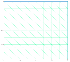
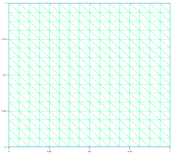
Note that, we can obtain the convergence orders for p(tn)pnp(t^{n})-p^{n} as epne_{p}^{n} based on the properties of Lagrange interpolation [34]. The errors for 𝐮\mathbf{u} and qq are defined in a similar way. We denote the error in energy norm for the displacement 𝐮n\mathbf{u}^{n} by |e𝐮n|2=ε(e𝐮n)2|||e_{\mathbf{u}}^{n}|||^{2}=||\varepsilon(e_{\mathbf{u}}^{n})||^{2}. For the square domain, the uniform triangular mesh is employed, and Figure 1 shows the computational grid with the meshes.

Refer to caption
(a)  
Refer to caption
(b)  
Fig. 1: The space meshes: (a) h=1/8, (b) h=1/16
Example 1.

Let the domain be Ω=(0,1)2\Omega=(0,1)^{2} and T¯=1\bar{T}=1. Then, we choose the Dirichlet boundary ΓD=Ω\Gamma_{D}=\partial\Omega and the exact solutions

𝐮=t2[sin(πx)cos(πy)cos(πx)sin(πy)]\mathbf{u}={t^{2}\left[\begin{array}[]{c}\sin(\pi x)\cos(\pi y)\\ \cos(\pi x)\sin(\pi y)\end{array}\right]}

and

p=etsin(πx)sin(πy).p=e^{-t}\sin(\pi x)\sin(\pi y).

The body force function 𝐟\mathbf{f}, the forced fluid gg, initial conditions and Dirichlet boundary conditions are determined by the exact solutions. We obtain

𝐮=2πt2cos(πx)cos(πy).\nabla\cdot\mathbf{u}=2\pi t^{2}\cos(\pi x)\cos(\pi y).

We set the parameters κ=1.0\kappa=1.0, μ=1.0\mu=1.0 and λ=102\lambda=10^{-2} in this example. Table 1 gives the error estimates with respect to hh for ([P2]2,P0,P1)([P_{2}]^{2},P_{0},P_{1}) elements. The convergence orders for each variable are consistent with our theory. Table 2 shows the convergence orders with ([P2]2,P1,P1)([P_{2}]^{2},P_{1},P_{1}) elements, which are in agreements with our results in Theorem 9. Furthermore, the convergence orders with respect to τ\tau can be observed in Table 3 and Table 4.

Moreover, the convergence orders for the pressure epn\|\nabla e_{p}^{n}\| are computed to be O(h2)O(h^{2}) in Table 1 and Table 2, so we can obtain convergence results O(h)O(h) for (p(tn)pn)\|\nabla(p(t^{n})-p^{n})\| due to the properties of the linear Lagrange interpolation. A similar argument can be employed for the pressure in H1H^{1} norm as well. In particular, the convergence orders of O(h2)O(h^{2}) for the displacement 𝐮\mathbf{u} and the pressure in L2L^{2} norm can be observed in Tables 1 and 2.

h |e𝐮n||||e_{\mathbf{u}}^{n}||| e𝐮n||e_{\mathbf{u}}^{n}|| eqn||e_{q}^{n}|| epn||\nabla e_{p}^{n}|| epn||e_{p}^{n}||
error order error order error order error order error order
1/8 1.2572e-02 4.1887e-04 1.0502e-02 7.8321e-02 1.6727e-02
1/16 5.7283e-03 1.1340 9.7376e-05 2.1048 2.5910e-03 2.0190 1.9241e-02 2.0252 4.1523e-03 2.0101
1/32 2.8055e-03 1.0298 2.3932e-05 2.0246 6.4557e-04 2.0048 4.7886e-03 2.0065 1.0362e-03 2.0026
1/64 1.3961e-03 1.0068 5.9561e-06 2.0065 1.6128e-04 2.0010 1.1959e-03 2.0015 2.5896e-04 2.0005
Table 1: Convergence at tn=1t^{n}=1 when τ=h2\tau=h^{2} for ([P2]2,P0,P1)([P_{2}]^{2},P_{0},P_{1}): Dirichlet boundary
h |e𝐮n||||e_{\mathbf{u}}^{n}||| e𝐮n||e_{\mathbf{u}}^{n}|| eqn||e_{q}^{n}|| epn||\nabla e_{p}^{n}|| epn||e_{p}^{n}||
error order error order error order error order error order
1/8 3.8777e-03 3.0217e-04 2.8315e-03 1.0661e-02 2.3541e-03
1/16 6.8421e-04 2.5026 7.7262e-05 1.9675 7.2470e-04 1.9661 2.6829e-03 1.9904 6.0092e-04 1.9699
1/32 1.4486e-04 2.2397 1.9575e-05 1.9807 1.8225e-04 1.9914 6.7188e-04 1.9975 1.5103e-04 1.9923
1/64 3.4293e-05 2.0786 4.9123e-06 1.9945 4.5631e-05 1.9978 1.6804e-04 1.9993 3.7807e-05 1.9981
Table 2: Convergence at tn=1t^{n}=1 when τ=h2\tau=h^{2} for ([P2]2P1,P1)([P_{2}]^{2}P_{1},P_{1}): Dirichlet boundary
τ\tau |e𝐮n||||e_{\mathbf{u}}^{n}||| e𝐮n||e_{\mathbf{u}}^{n}|| eqn||e_{q}^{n}|| epn||\nabla e_{p}^{n}|| epn||e_{p}^{n}||
error order error order error order error order
1 3.8459e-03 2.4103e-03 1.5573e-01 3.3603e-01 1.5887e-01
1/2 1.9797e-03 0.9580 1.2156e-03 0.9875 7.8538e-02 0.9875 1.6971e-01 0.9855 8.0238e-02 0.9854
1/4 1.0634e-03 0.8965 6.0752e-04 1.0006 3.9277e-02 0.9997 8.5072e-02 0.9963 4.0241e-02 0.9956
1/8 6.5722e-04 0.6942 3.0332e-04 1.0020 1.9639e-02 0.9999 4.2737e-02 0.9931 2.0245e-02 0.9911
Table 3: Convergence at tn=1t^{n}=1 when h=1/64h=1/64 for ([P2]2,P0,P1)([P_{2}]^{2},P_{0},P_{1}): Dirichlet boundary
τ\tau |e𝐮n||||e_{\mathbf{u}}^{n}||| e𝐮n||e_{\mathbf{u}}^{n}|| eqn||e_{q}^{n}|| epn||\nabla e_{p}^{n}|| epn||e_{p}^{n}||
error order error order error order error order
1 1.2052e-02 1.7118e-03 2.9200e-02 2.7565e-01 2.9310e-02
1/2 6.0467e-03 0.9950 8.5831e-04 0.9959 1.4653e-02 0.9947 1.3831e-01 0.9949 1.4713e-02 0.9943
1/4 3.0175e-03 1.0027 4.2802e-04 1.0038 7.3185e-03 1.0015 6.9128e-02 1.0005 7.3538e-03 1.0005
1/8 1.5027e-03 1.0057 2.1286e-04 1.0077 3.6508e-03 1.0033 3.4532e-02 1.0013 3.6736e-03 1.0012
Table 4: Convergence at tn=1t^{n}=1 when h=1/64h=1/64 for ([P2]2,P1,P1)([P_{2}]^{2},P_{1},P_{1}): Dirichlet boundary
Example 2.

We consider the problem as in Example 1 with Neumann and Dirichlet boundary conditions. Let the Neumann boundary be ΓN={(x,y)x=1,0<y<1}\Gamma_{N}=\{(x,y)\mid x=1,0<y<1\} and the Dirichlet boundary ΓD=ΩΓN\Gamma_{D}=\partial\Omega\setminus\Gamma_{N}.

We also set the parameters κ=1.0\kappa=1.0, μ=1.0\mu=1.0 and λ=102\lambda=10^{-2} as in Example 1. With the Neumann and Dirichlet boundary conditions, we observe the convergence orders in energy norm of the displacement in Table 5 and Table 6 which are in full agreements with our main results in Theorem 8 and Theorem 9. The convergence orders O(h2)O(h^{2}) for the total stress in L2L^{2} norm are recorded in Table 5 and Table 6 which confirm our theory.

h |e𝐮n||||e_{\mathbf{u}}^{n}||| e𝐮n||e_{\mathbf{u}}^{n}|| eqn||e_{q}^{n}|| epn||\nabla e_{p}^{n}|| epn||e_{p}^{n}||
error order error order error order error order error order
1/8 1.4182e-02 1.7411e-03 1.2276e-02 8.0666e-02 1.8625e-02
1/16 5.9152e-03 1.2615 4.1226e-04 2.0783 3.0872e-03 1.9914 2.0045e-02 2.0087 4.6735e-03 1.9946
1/32 2.8262e-03 1.0655 9.9754e-05 2.0471 7.6655e-04 2.0098 4.9844e-03 2.0077 1.1632e-03 2.0064
1/64 1.3985e-03 1.0149 2.4612e-05 2.0190 1.9134e-04 2.0022 1.2446e-03 2.0017 2.9050e-04 2.0014
Table 5: Convergence at tn=1t^{n}=1 when τ=h2\tau=h^{2} for ([P2]2,P0,P1)([P_{2}]^{2},P_{0},P_{1}): Neumann and Dirichlet boundary
h |e𝐮n||||e_{\mathbf{u}}^{n}||| e𝐮n||e_{\mathbf{u}}^{n}|| eqn||e_{q}^{n}|| epn||\nabla e_{p}^{n}|| epn||e_{p}^{n}||
error order error order error order error order error order
1/8 6.0055e-03 6.2900e-04 2.5456e-03 1.5738e-02 2.2821e-03
1/16 1.1116e-03 2.4336 1.6328e-04 1.9457 6.5647e-04 1.9914 3.9863e-03 1.9811 5.8439e-04 1.9653
1/32 2.2324e-04 2.3159 4.1244e-05 1.9850 1.6542e-04 2.0098 9.9993e-04 1.9951 1.4701e-04 1.9910
1/64 4.8554e-05 2.2009 1.0324e-05 1.9981 4.1437e-05 2.0022 2.5020e-04 1.9987 3.6809e-05 1.9977
Table 6: Convergence at tn=1t^{n}=1 when τ=h2\tau=h^{2} for ([P2]2,P1,P1)([P_{2}]^{2},P_{1},P_{1}): Neumann and Dirichlet boundary
Example 3.

Let the domain be Ω=(0,1)2\Omega=(0,1)^{2} and T¯=1\bar{T}=1. The Dirichlet boundary satisfy ΓD=Ω\Gamma_{D}=\partial\Omega. Then, we choose the exact solutions

𝐮=et[sin(2πy)(1+cos(2πx))+1μ+λsin(πx)sin(πy)sin(2πx)(1cos(2πy))+1μ+λsin(πx)sin(πy)]\mathbf{u}=e^{-t}{\left[\begin{array}[]{c}\sin(2\pi y)(-1+\cos(2\pi x))+\frac{1}{\mu+\lambda}\sin(\pi x)\sin(\pi y)\\ \sin(2\pi x)(1-\cos(2\pi y))+\frac{1}{\mu+\lambda}\sin(\pi x)\sin(\pi y)\end{array}\right]}

and

p=etsin(πx)sin(πy).p=e^{-t}\sin(\pi x)\sin(\pi y).

We choose the body force function 𝐟\mathbf{f}, forced fluid gg, initial conditions and Dirichlet boundary conditions so that the exact solutions satisfy the problems (1) and (2) . Note that 𝐮=πetsin(π(x+y))/(μ+λ)\nabla\cdot\mathbf{u}=\pi e^{-t}\sin(\pi(x+y))/(\mu+\lambda), and when the elastic Lame´\acute{e} parameters λ\lambda\rightarrow\infty, we have 𝐮0\nabla\cdot\mathbf{u}\rightarrow 0.

We set the parameters κ=1.0\kappa=1.0, μ=1.0\mu=1.0 and λ=104\lambda=10^{4} with nearly incompressible case. We test both ([P2]2,P0,P1)([P_{2}]^{2},P_{0},P_{1}) and ([P2]2,P1,P1)([P_{2}]^{2},P_{1},P_{1}) elements to emphasize the efficiency. Thus, Table 7 and Table 8 show the convergence orders for each variable as expected. At the same time, the convergence orders O(h2)O(h^{2}) for the total stress eqn\|e_{q}^{n}\| are shown in Table 7, and we can observe that the convergence orders of displacement |e𝐮n||||e_{\mathbf{u}}^{n}||| are O(h3)O(h^{3}) in Table 8 which is better than expected. Therefore, we can conclude that the finite element method is valid for the nearly incompressible case.

h |e𝐮n||||e_{\mathbf{u}}^{n}||| e𝐮n||e_{\mathbf{u}}^{n}|| eqn||e_{q}^{n}|| epn||\nabla e_{p}^{n}|| epn||e_{p}^{n}||
error order error order error order error order error order
1/8 4.8359e-02 1.1460e-03 1.0101e-02 1.0998e-02 2.3094e-03
1/16 1.9701e-02 1.2955 2.0102e-04 2.5111 2.6388e-03 1.9365 2.8017e-03 1.9728 5.9488e-04 1.9568
1/32 9.7854e-03 1.0095 4.9100e-05 2.0335 7.3649e-04 1.8411 7.0387e-04 1.9929 1.4987e-04 1.9888
1/64 4.9240e-03 0.9908 1.2386e-05 1.9870 2.1109e-04 1.8028 1.7619e-04 1.9981 3.7540e-05 1.9972
Table 7: Convergence at tn=1t^{n}=1 when τ=h\tau=h for ([P2]2,P0,P1)([P_{2}]^{2},P_{0},P_{1}): Nearly incompressible case
h |e𝐮n||||e_{\mathbf{u}}^{n}||| e𝐮n||e_{\mathbf{u}}^{n}|| eqn||e_{q}^{n}|| epn||\nabla e_{p}^{n}|| epn||e_{p}^{n}||
error order error order error order error order error order
1/8 3.0635e-02 9.8803e-04 1.7083e-02 1.0998e-02 2.3094e-03
1/16 4.3311e-03 2.8223 6.9922e-05 3.8207 3.0093e-03 2.5050 2.8017e-03 1.9728 5.9488e-04 1.9568
1/32 5.6515e-04 2.9380 4.5564e-06 3.9397 7.0999e-04 2.0835 7.0388e-04 1.9929 1.4987e-04 1.9888
1/64 7.1810e-05 2.9763 2.8910e-07 3.9782 1.7635e-04 2.0093 1.7619e-04 1.9981 3.7540e-05 1.9972
Table 8: Convergence at tn=1t^{n}=1 when τ=h\tau=h for ([P2]2,P1,P1)([P_{2}]^{2},P_{1},P_{1}): Nearly incompressible case
Example 4.

We consider Example 3 with non-homogeneous Dirichlet boundary conditions. Let the domain be Ω=(0,1)2\Omega=(0,1)^{2} and T¯=1\bar{T}=1. The Dirichlet boundary satisfy ΓD=Ω\Gamma_{D}=\partial\Omega. Then, we choose the exact solutions

𝐮=et[sin(2y)(1+cos(2x))+1μ+λsin(x)sin(y)sin(2x)(1cos(2y))+1μ+λsin(x)sin(y)]\mathbf{u}=e^{-t}{\left[\begin{array}[]{c}\sin(2y)(-1+\cos(2x))+\frac{1}{\mu+\lambda}\sin(x)\sin(y)\\ \sin(2x)(1-\cos(2y))+\frac{1}{\mu+\lambda}\sin(x)\sin(y)\end{array}\right]}

and

p=etsin(x)sin(y).p=e^{-t}\sin(x)\sin(y).

Again, we choose the body force function 𝐟\mathbf{f}, forced fluid gg, initial conditions and Dirichlet boundary conditions so that the exact solutions satisfy the problems (1) and (2) . Note that 𝐮=etsin((x+y))/(μ+λ)\nabla\cdot\mathbf{u}=e^{-t}\sin((x+y))/(\mu+\lambda), and when the elastic Lame´\acute{e} parameters λ\lambda\rightarrow\infty, we have 𝐮0\nabla\cdot\mathbf{u}\rightarrow 0.

We also set the parameters κ=1.0\kappa=1.0, μ=1.0\mu=1.0 and λ=104\lambda=10^{4}. The results in Table 9 and Table 10 verify our theory for the case with non-homogeneous Dirichlet boundary conditions.

h |e𝐮n||||e_{\mathbf{u}}^{n}||| e𝐮n||e_{\mathbf{u}}^{n}|| eqn||e_{q}^{n}|| epn||\nabla e_{p}^{n}|| epn||e_{p}^{n}||
error order error order error order error order error order
1/8 2.5465e-03 5.9338e-05 1.1059e-03     . 1.6621e-04 3.6140e-05
1/16 1.3791e-03 0.8847 1.7079e-05 1.7967 3.4468e-04 1.6818 4.2208e-05 1.9774 9.2862e-06 1.9604
1/32 7.1729e-04 0.9430 4.6074e-06 1.8901 1.0408e-04 1.7275 1.0556e-05 1.9994 2.3293e-06 1.9951
1/64 3.6553e-04 0.9725 1.1977e-06 1.9436 3.0911e-05 1.7515 2.6206e-06 2.0100 5.7865e-07 2.0091
Table 9: Convergence at tn=1t^{n}=1 when τ=h\tau=h for ([P2]2,P0,P1)([P_{2}]^{2},P_{0},P_{1}): Nearly incompressible case with non-homogeneous Dirichlet boundary conditions
h |e𝐮n||||e_{\mathbf{u}}^{n}||| e𝐮n||e_{\mathbf{u}}^{n}|| eqn||e_{q}^{n}|| epn||\nabla e_{p}^{n}|| epn||e_{p}^{n}||
error order error order error order error order error order
1/8 2.8381e-04 9.5582e-06 4.3295e-04 1.6621e-04 3.6141e-05
1/16 3.8805e-05 2.8706 6.4511e-07 3.8891 1.0424e-04 2.0542 4.2209e-05 1.9773 9.2864e-06 1.9604
1/32 5.0463e-06 2.9429 4.1637e-08 3.9536 2.5944e-05 2.0064 1.0556e-05 1.9994 2.3293e-06 1.9952
1/64 6.4255e-07 2.9733 2.6417e-09 3.9783 6.4796e-06 2.0014 2.6206e-06 2.0100 5.7866e-07 2.0091
Table 10: Convergence at tn=1t^{n}=1 when τ=h\tau=h for ([P2]2,P1,P1)([P_{2}]^{2},P_{1},P_{1}): Nearly incompressible case with non-homogeneous Dirichlet boundary conditions

5 Conclusions

For Biot’s consolidation model, we analyze the error estimates for a three field discretization. And the total stress coupling between the solid and fluid variable is as an unknown. Moreover, the convergence of fully-discrete scheme is presented and the results can be extended to many finite element spaces that satisfy the inf-sup conditions.

References

  • [1] M.A. Biot, General theory of three-dimensional consolidation, J. Appl. Phys. vol. 12(1941)pp. 155-164.
  • [2] M. A. Biot, Theory of Elasticity and Consolidation for a Porous Anisotropic Solid, J. Appl. Phys. vol.26(1955)pp. 182-185.
  • [3] H. Soltanzadeh, C.D. Hawkes and J.S. Sharma, Poroelastic model for production-and injection-induced stresses in reservoirs with elastic properties different from the surrounding rock, International Journal of Geomechanics vol. 7(2007)pp. 353-361.
  • [4] T. Nagashima, T. Shirakuni, S. I. Rapoport, A two-dimensional, finite element analysis of vasogenic brain edema, Neurol. med. chir. vol. 30(1990)pp. 1-9.
  • [5] C. C. Swan, R. S. Lakes, R. A. Brand, K. Stewart, Micromechanically based poroelastic modeling of fluid flow in Haversian bone, J. Biomech. Eng. vol. 125(2003)pp. 25-37.
  • [6] R. W. Lewis, Y. Sukirman, Finite element modelling of three‐phase flow in deforming saturated oil reservoirs, Intl. J. for Num. and Anal. Methods in Geomech. vol. 17(1993)pp. 577-598.
  • [7] P. A. Netti, L. T. Baxter, Y. Boucher, R. Skalak, R. K. Jain, Macro-and microscopic fluid transport in living tissues: Application to solid tumors, AIChE Journal of Bioengineering Food, and Natural Products vol. 43(1997))pp. 818-834.
  • [8] R. E. Showalter, Diffusion in poro-elastic media, J. Math. Anal. Appl. vol. 251(2000)pp. 310-340.
  • [9] R. Leiderman, P. Barbone, A. Oberai, and J. Bamber, Coupling between elastic strain and interstitial fluid flow: ramifications for poroelastic imaging, Phys. Med. Biol. vol. 51(2006)pp. 6291-6313.
  • [10] Y. Yokoo, K. Yamagata, H. Nagaoka, Finite element method applied to Biot’s consolidation theory, Soils and Foundations vol. 11(1971)pp. 29-46.
  • [11] A. Zˇ\check{Z}eni´\acute{i}sˇ\check{s}ek, The existence and uniqueness theorem in Biot’s consolidation theory, Aplikace matematiky vol. 29(1984)pp. 194-211.
  • [12] M. A. Murad, A. F. D. Loula, Improved accuracy in finite element analysis of Biot’s consolidation problem, Compur. Methods Appl. Mech. Eng. vol. 95(1992)pp. 359-382.
  • [13] M. A. Murad, A. F. D. Loula, On stability and convergence of finite element approximations of Biot’s consolidation problem, Internat. J. Numer. Methods Engrg. vol. 37(1994)pp. 645-667.
  • [14] M. A. Murad, V. Thome´\acute{e}e, A.F.D.Loula, Asymptotic behavior of semidiscrete finite-element approximations of Biot’s consolidation problem, SIAM J. Numer. Anal. vol. 33(1996)pp. 1065 -1083.
  • [15] J. Korsawe, G. Starke, A least-squares mixed finite element method for Biot’s consolidation problem in porous media, SIAM J. NUMER. ANAL. vol. 43(2005)pp. 318-339.
  • [16] P. J. Phillips, M. F. Wheeler, A coupling of mixed and continuous Galerkin finite element methods for poroelasticity I: the continuous in time case Comput. Geosci. vol. 11(2007)pp. 131-144.
  • [17] P. J. Phillips, M. F. Wheeler, A coupling of mixed and discontinuous Galerkin finite-element methods for poroelasticity, Comput. Geosci. vol. 12 (2008)pp. 417-435.
  • [18] Y. Chen , Y. Luo , M. Feng, Analysis of a discontinuous Galerkin method for the Biot’s consolidation problem, Appl. Math. Comput. vol. 219(2013)pp. 9043-9056.
  • [19] M. Wheeler, G. Xue , I. Yotov, Coupling multipoint flux mixed finite element methods with continuous Galerkin methods for poroelasticity, Computational Geosciences vol. 18(2014)pp. 57-75.
  • [20] S.-Y.Yi, Convergence analysis of a new mixed finite element method for Biot’s consolidation model, Numer. Meth. Part. Differ. Equ. vol. 30(2014)pp. 1189–1210.
  • [21] S.-Y. Yi, A study of two modes of locking in poroelasticity, SIAM J. Numer. Anal. vol. 55(2017)pp. 1915-1936.
  • [22] J. J. Lee, Robust error analysis of coupled mixed methods for Biot’s consolidation model, J. Sci. Comput. vol. 69(2016)pp. 610-632.
  • [23] X. Hu, C. Rodrigo, F. J. Gaspar, L. T. Zikatanov, A nonconforming finite element method for the Biot’s consolidation model in poroelasticity, J. Comput. Appl. Math. vol. 310(2017)pp. 143-154.
  • [24] Q. Hong, J. Kraus, Parameter-robust stability of classical three-field formulation of Biot’s consolidation model, Electron. Trans. Numer. Anal. vol. 48(2018)pp. 202–226.
  • [25] G. Chen, M. Feng, Stabilized Finite Element Methods for Biot’s Consolidation Problems Using Equal Order Elements, Adv. Appl. Math. Mech. vol. 10(2018)pp. 77-99.
  • [26] G. Kanschat, B. Riviere, A finite element method with strong mass conservation for Biot’s linear consolidation model, J. Sci. Comput. vol. 77(2018)pp. 1762-1779.
  • [27] R. Oyarzu´\acute{u}a, R. Ruiz-Baier, Locking-free finite element methods for poroelasticity, SIAM J. Numer. Anal. vol. 54(2016)pp. 2951-2973.
  • [28] J. J. Lee, K. A. Mardal, R. Winther, Parameter-robust discretization and preconditioning of Biot’s consolidation model, SIAM J. Sci. Comput. vol. 39 (2017)pp. A1-A24.
  • [29] J. J. Lee, E. Piersanti, K. A. Mardal, M. E.Rognes, A mixed finite element method for nearly incompressible multiple-network poroelasticity, SIAM J. Sci. Comput. vol. 41 (2019)pp. A722-A747.
  • [30] S. C. Brenner, L. R. Scott, The mathematical theory of finite element methods. Springer Science & Business Media, Third edition. 2007.
  • [31] P. G. Ciarlet, The finite element method for elliptic problems, North-Holland, New York, 1978.
  • [32] J.A. Nitsche, On Korn’s second inequality, RAIRO Anal. Numer. vol. 15(1981)pp. 237-248.
  • [33] S. C. Brenner, Korn’s inequalities for piecewise H1H^{1} vector fields, Math. Comput. vol. 73(2004)pp. 1067-1087.
  • [34] A. Quarteroni, A. Valli, Numerical Approximation of Partial Differential Equations, Springer Science & Business Media. 2008.
  • [35] V. Girault and P.-A. Raviart, Finite Element Approximation of the Navier–Stokes Equations, Lecture Notes in Math. 749, Springer-Verlag, Berlin, New York, 1979.
  • [36] F. Brezzi, M. Fortin, Mixed and Hybrid Finite Element Methods, Springer Science & Business Media, 1991.