Finite Difference Solution Ansatz approach in Least-Squares Monte Carlo
Abstract
This article presents a simple but effective and efficient approach to improve the accuracy and stability of Least-Squares Monte Carlo for American-style option pricing as well as expected exposure calculation in valuation adjustments. The key idea is to construct the ansatz of conditional expected continuation payoff using the finite difference solution from one dimension, to be used in linear regression. This approach bridges between solving backward partial differential equations and Monte Carlo simulation, aiming at achieving the best of both worlds. Independent of model settings, the ansatz is proved to serve as a control variate to reduce the least-squares errors. We illustrate the technique with realistic examples including Bermudan options, worst of issuer callable notes and expected positive exposure on European options. The method can be considered as a generic numerical scheme across various asset classes, in particular, as an accurate method for pricing and risk-managing American-style derivatives under arbitrary dimensions.
Key Words: Least-squares regression, finite difference method, partial differential equations, Bermudan option, worst of issuer callable note, credit value adjustment, high-dimensional derivative pricing
1 Introduction
Solving partial differential equations (PDE) with finite difference methods and Monte Carlo simulation are two major advanced numerical methods for exotic derivative pricing among practitioners. As the dimensionality of the problem increases, the PDE approach becomes less feasible due to implementation complexity and the numerical burden; specifically, there is no efficient and accurate implementation widely accepted in the industry with dimension greater than two. On the other hand, the Monte Carlo method is widely used in high-dimensional derivative pricing without suffering from the ‘curse of dimensionality’ as PDE with grid approach does.
Derivatives with American-style early exercise features are especially difficult to price within Monte Carlo framework. The major challenge is the determination of the conditional expectation future payoff for an optimal exercise strategy, without further additional numerical procedures which cannot be obtained in a simple forward simulation. With this regard, a backward PDE solver seems outwit Monte Carlo method in low dimensions, as the former effectively stores conditional expectation payoff within the PDE grids when marching backward.
Among pioneers to tackle this challenge within simulation framework(Barraquand & Martineau, (1995); Broadie & Glasserman, (2004); Tsitsiklis & Van Roy, (2001); Longstaff & Schwartz, (2001)), the least-squares Monte Carlo approach (Longstaff & Schwartz, (2001)), is the most popular algorithm due to its reliability and robustness(Stentoft, (2001)). The breakthrough is to allow efficient computation of conditional expectation of future payoff by a projection towards a given set of basis functions. One important detail to note is that the least-squares projection proxy is only used in the optimal stopping time determination, rather than in the value function evaluation itself, another variant of regression-based simulation approach proposed by Tsitsiklis & Van Roy, (2001). It has been showed that, by Stentoft, (2014), the former algorithm achieves much less bias in absolute terms in comparison, in either two-period or multiple-period settings. Further theoretical analysis proved the almost sure convergence of the algorithm and the rate of convergence by combining simulation and least-squares method is asymptotically Gaussian normalized error (Clément et al., (2002)).
After this milestone supported by solid theoretical foundation, there has been active research about further improvement on the least-squares method as main stream for American-style option pricing under arbitrary dimensions. For example, conventional variance reduction techniques applicable to European-style option pricing, e.g., antithetic variates, control variates and moment matching methods, were soon proved effective in least-squares Monte Carlo, by reducing the statistical error of finite samples in the payoff expectation estimator Tian & Burrage, (2003). After these achievements as low-hanging fruits, further focus has been skewed towards an enhanced estimator of conditional expectation until more recently. There have been diverse research activities with specific issues to tackle: Fabozzi et al., (2017) suggested a weighted regression approach to manage heteroskedasticity in the regression; and in order to eliminate the foresight bias introduced from an in-sample method, Boire et al., (2022) and Woo et al., (2024) proposed different bias-adjusted corrections in the least-squares estimator, without doubling simulations. Worth to mention that the out-of-sample implementation, i.e., additional independent simulation paths for regression only, is a much more robust alternative to address these statistical defects.
Concurrently, there has been growing interest in developing efficient high-dimensional PDE solvers, particularly with the emergence of machine learning techniques, such as deep neural network (DNN) methods. The idea is to cast the high-dimensional PDE solving problem as a learning task, where a DNN is trained to fit the particular setting (Han et al., (2018)). As applications to optimal stopping problems, effective forward DNN with reduced loss function and accelerated convergence speed to solve backward stochastic differential equations (BSDEs) have been proposed by Fujii & Takahashi, (2019) in American basket option pricing. Later, backward deep BSDEs method to better tackle the optimal stopping problem was proposed by Liang et al., (2021); Gao et al., (2023). However, none of these studies so far were able to provide convincing evidence that DNN methods outperform the least-squares method in terms of accuracy, stability and efficiency. For instance, when pricing Bermudan option with 5-10 underlyings, DNN approach is 5 time slower than least-squares Monte Carlo while achieving similar accuracy; it is only when beyond 20 underlyings that the DNN approach has the edge over simulation methods in terms of memory efficiency (Liang et al., (2021)). The advantage of the DNN approach in terms of memory efficiency has become less pronounced, as the continuous improvement of hardware has made larger memory capacities more readily available. While the DNN-based approaches hold promise, the least-squares method remains a more robust and competitive alternative.
In this paper, we propose an enhanced least-squares regression based method by Longstaff & Schwartz, (2001), in particular, which aims at improving the projection of conditional expectations by constructing an ansatz from a finite difference PDE solver, to be used in the linear regression. Previous studies in the literature have explored methodologies that aim to combine PDE-based and simulation-based approaches, to leverage the strengths of both. For instance, Farahany et al., (2020) introduced a method by mixing a Fourier transforms based PDE solver on discretized volatility space and regressing the value function onto these resulting conditional payoff profiles, under stochastic volatility model. However, our work is distinguished from their proposal in below aspects:
-
•
Our method is suitable under generic model settings, not limited to stochastic volatility only.
- •
Therefore, our approach is the first attempt at integrating a PDE solver into least-squares Monte Carlo framework, to aid conditional expectation evaluation within optimal stopping time approximation, to the best of our knowledge.
Going beyond American-style derivatives pricing, the regression-based approach is also widely used in the context of Credit Valuation Adjustment (CVA), which has been imposed under the Basel III framework as risk capital charge. For CVA, as well as other related value adjustments such Debt Value Adjustment (DVA), Funding Value Adjustment (FVA) and Capital Value Adjustment (KVA), all of which are now categorized as Valuation Adjustments (XVA) in a general term, the major challenge is the determination of uncertain future exposures of a given transaction. Instead of a brute-force approach to re-evaluate the entire portfolio in each simulated scenario, a practically prevalent approach in the industry is to approximate the financial product mark-to-market values using regression functions via the celebrated least-squares approach. As we can see later, the call for stability, on top of accuracy, on the regression method, plays an important role in this application within this regard, and our new method is also readily applicable to satisfy the requirement.
The rest of this paper is organized as follows. In Sec.2, we introduce basic background knowledge for option pricing in the context of American-style exercise derivatives, e.g., Bermudan options and worst of issuer callable note, and the Expected Positive Exposure calculation in XVA. Then we outline prevailing numerical methods in practice, including the least-squares Monte Carlo approach in Sec.2.3, and finite difference PDE method in Sec.2.4. With such foundation, we will proceed to introduce our novel approach in Sec.2.5 from a model-independent assumption. Then underlying model settings and implementation details will be given in Sec.2.6 and Sec.2.7, respectively. Numerical results for Bermudan options and worst of issuer callable notes are presented in Sec.3, which examines the accuracy of various available methods. The expected positive exposure (EPE) and CVA calculation on European option are also presented. Finally, concluding remarks are given in Sec.4.
2 Theoretical Framework
First of all, we assume that throughout a given terminal expiry , there is a complete probability space () satisfying the usual conditions with respect to which all processes are defined under risk-neutral measure , relevant for derivative valuation as well as regulatory CVA computations. We denote by the riskless interest rate.
2.1 Option Pricing with American-style exercise
We assume that the American-style option is exercisable after (excluding) and up to (including) the final expiry for every time interval . We define the set of exercise times on or after as . The exercisability is either on the option holder side or on the issuer side. Within the complete probability space , there exists a discrete filtration on . For notational clarity, we use to denote a stochastic variable under with . In this spirit, the state variables are denoted by , which is -measurable.
To unambiguously describe an American-style option, we have to define two important quantities: as the exercise payoff at , and as the sum of discounted (back to ) future cash flows from (exclusively) and up to a stopping time . Different from or , is measurable up to . For single cash flow derivative, these two quantities are related to each other as for .
Now one can define the expected option value, i.e., present value (PV), as
| (2.1) |
Similar to previous literature, we limit the attention to square integrable payoff functions, i.e., . Let denote the space of square integrable functions. In this article, we take Bermudan options on constant-weighted basket with (see Appendix A.1), and worst of issuer callable notes (WIC) on worst-of basket (see Appendix A.2), respectively. Here the underlying basket is dimensional and are asset spot prices.
Under discrete-time formulation, a preferable way to solve the Eqn.2.1 is to find out the optimal stopping time strategy, denoted by (removing the tilde compared to for optimality and omitting the dependence on for notational convenience). For further notational clarity, we also introduce to represent the option path value under optimal stopping times , differentiated from by removing the tilde similarly to emphasize that it is calculated under optimal stopping times .
With the help of , we further define the so-called continuation value representing the conditional expected option value upon exercising strictly after, and discounted back to, as
| (2.2) |
Thanks to the -measurability of in the same way as , the formal solution of the optimal stopping times can be written as, via a dynamic programming fashion (together with terminal condition ),
| (2.3) |
where the exercise indicator function is defined as , with Heaviside step function denoted by and ‘’(‘’) for holder (issuer) exercise. The formal dynamic programming solution of is also given by
| (2.4) |
2.2 Credit Value Adjustment and Expected Positive Exposure
For the ease of illustration without loss generality, we have assumed that the product doesn’t have early termination features, eg. European Option on . We define the Credit value adjustment (CVA) on a financial transaction as the expected loss resulting from the potential future default of the counterparty, given by:
| (2.5) |
where is the recovery rate and denotes the default probability of the counterparty at , which depends on the counterparty hazard rate denoted by . Furthermore, is the mark-to-market value of the option at .
We define the Expected Positive Exposure (EPE), as well as its discounted version EPE*, as:
| (2.6) |
Here we re-use the same notation defined in previous subsection, to represent the option value before expiry . Efficient computation of is of prime importance in the calculation of CVA and other XVA’s, where the difficulty in practice arises from the lack of analytical tractability in many cases.
To further take into account the Wrong Way Risk (WWR), we consider a hazard rate with a general functional dependence on (Hull & White, (2012)):
where and are WWR model parameters.
2.3 Least-Squares Monte Carlo method
As can be seen from above, once the -measurable conditional expectations in Eqn.2.2 and Eqn.2.6 can be efficiently crystallized into a functional form , the optimal stopping times in American style option pricing and EPE/CVA calculation, can be determined in a path-by-path manner independently. The core idea of regression based Least-Squares approach (LSM) is to assume this functional form can be decomposed as a linear combination of a set of basis functions , where the linear coefficients are obtained via regression using the cross-sectional information computed in the simulation.
For notation convenience, let’s define the least-squares estimator of the continuation value using the projection operator at upon option value under basis functions in space, as
| (2.7) |
where
| (2.8) |
It means that are to be obtained via regression using the cross-sectional information computed in the simulation as described in Appendix A.3. in above is the objective function to be minimized, whose lower bound is given by, in the limit of being exact:
| (2.9) |
where denotes the conditional variance.
In Eqn.2.7, the least-squares estimator is also called regressed continuation value.
After solving for all recursively backward in time from maturity, are fully determined. Then with a forward pricing Monte Carlo, one can then compute PV as
where the superscript indicates that the variable is under of the total pricing paths; and the optimal stopping rule is to only exercise the option at
| (2.10) |
To have a better convergence and calculation efficiency, one usually draws a different set of Monte Carlo paths in this pricing stage more than the previous regression stage to determine the continuation value, i.e., . This is so-called out-of-sample implementation to eliminate foresight bias without the need of sophisticated regression correctors as mentioned before.
As an analogy of the EPE in the CVA problem is calculated as (by replacing the value function with least-squares estimator)111Note that we are aware of alternative hybrid approach to calculate EPE, by making use of both the simulated cash flows and regressed function (Joshi & Kwon, (2016)). The drawback of this proposal is that one has to generate all the cash flows at given individual product level, without being decoupled from the path generation at upper portfolio level. It would result in an aggregation of contractual timelines, rather than simple algorithmic operation upon regressed functions at product level when it comes to portfolio aggregation. :
| (2.11) |
Similarly, the Monte Carlo estimator of CVA can be defined accordingly as:
| (2.12) |
2.3.1 Basis function and Limitations
The basis functions , also known as regressors, are the main source of approximation within LSM. Based on the original study, the LSM is remarkably robust to the choice of basis functions (Longstaff & Schwartz, (2001)). However, in a further analysis, it is concluded that for complex options, the robustness does not seem to be guaranteed. Nevertheless, there is no golden rule provided by the author as an optimal choice for any given product, and different choices of popular regressors can merely affect option prices slightly (Moreno, (2003)).
In practice, it is not worth using special functions involving exponential calculation, such as Laguerre, or Hermite polynomials, as they introduce unnecessary computational burden without actual benefit. Thus, simple monomials are widely used in LSM as regressors, i.e., in the case of single state variable222It can be easily generalized to the case of multiple state variables, e.g., in the case of stochastic volatility, by specifying the total monomial degree across variables.. There are several limitations as follows:
-
•
With increasing the cutoff for the sake of regression accuracy, it becomes more susceptible to overfitting.
-
•
The fitting accuracy is poor away from at-the-money (ATM), as those regions are effectively out of scope in the objective function to be minimized.
-
•
As a solution of backward recursive optimization, would depend on the solution of the counterpart at , which was obtained by another regression. That said, the numerical error propagates and accumulates from iteration to iteration.
2.4 Finite difference approach in PDE
Alternative approach to solve the American-style option pricing is the finite difference (FD) method. The elegance of FD method is that it marches from maturity to present, which naturally fits into the requirement of backward recursive optimization in stopping time problems. We restrict the discussion within low-dimensional only, i.e., 1D, for maximum efficiency and accuracy. The most generic model reliable in replicating the market characteristics and solvable under 1D FD PDE is the local volatility, under which the option price as function of underlying spot and time satisfies:
| (2.13) |
within the time domain , and subjected to the initial condition and transition conditions around due to obstacle problem as
for holder’s exercise; and
for issuer’s exercise, respectively. As we can see later in Sec.2.6, and in Eqn.2.13 corresponds to the continuous dividend yield and local volatility for a single asset, respectively.
After solving the 1D backward propagating PDE via Crank-Nicolson method, we will denote by, from now on, the FD solution of continuation value at , which is related to backward PDE solution as
| (2.14) |
2.5 FD Solution Ansatz based Least-Squares Monte Carlo
Before proceeding, we introduce below proposition:
Proposition 1.
In a generalized LSM formulism, the continuation value estimator is exact if the exact continuation value is used as the only regressor.
The proof of Prop.1 is omitted as it is an elementary consequence of conditional expectation as projection that minimizes the objective function of LSM. This conclusion is free from model setting assumption.
For a general problem of interest, one could find an auxiliary variable with existing exact (or quasi-exact) solution as an ansatz to start with as one of the basis functions in the projection, with the expectation of dominating regression weight on this ansatz in the spirit of Prop.1. Inspired by the simplicity of FD solution for 1D PDE in Sec.2.4 with efficiency and quasi-exact accuracy, we would intuitively take the option price under 1D process as auxiliary variable, whose FD solution of continuation value is given by Eqn.2.14. From now on, we call this new method by incorporating into one of the LSM basis functions as FD Solution Ansatz based Least-Squares Monte Carlo (FD-LSM).
Mathematically, FD-LSM is defined by a modified least-squares continuation estimator with a new projection operator , as opposed to the classic one (previously denoted by defined in Eqn.2.7) operating on (previously denoted by ). The new basis functions of is given by as a union of and ( is decremented by one to cater for the added new FD ansatz), where 333We allow a constant term in the regressors to cater for mismatch of center of mass between independent and dependent variables. under which the associated projection operator is also introduced for illustrative purpose later.
Below proposition is established for the illustration of fundamental improvement of over from a theoretical point of view.
Proposition 2.
FD-LSM is equivalent to LSM with a modified projection kernel using the FD-solvable option value as a control variate.
Proof.
For notational convenience on random variables, we suppress the spatial dependence and condense the notation by replacing arguments depending on time by subscripts and further replace with simply , and thus .
For a given time step , we would like to derive the relation between and .
First of all, let’s denote by the FD solvable auxiliary variable with the interpretation as the path option value under 1D process satisfying . It is the equivalent counterpart of but under a hypothetical 1D simulation process instead.
By projecting the original option price into , we have
where from simple linear regression, the optimal coefficients are given by
| (2.15) |
with and denoting the conditional variance and covariance operators, respectively.
Applying the projection to gives
| (2.16) |
where in the last line, the constant term has been absorbed into .
In the limit of , we have due to convergence in LSM. Thus we arrive at the desired result as a consequence of linearity property of projection:
| (2.17) |
which claims that is equivalent to a customized on a control-variated kernel with the help of the FD ansatz. ∎
Based on Prop.2, proof of convergence on LSM from previous studies (Longstaff & Schwartz, (2001); Stentoft, (2001)) is equally applicable to FD-LSM. As , both and converge to the exact continuation function and are thus unbiased estimators. However, the variance of projection kernel in the former is reduced tremendously in a control variated manner by observing
| (2.18) |
with
defining the correlation between and .
Considering Eqn.2.9 together with above, one can see that least-squares error (lower bound) in FD-LSM is also reduced by the same scaling factor as the variance:
| (2.19) |
There are several further remarks on this result:
-
•
It is well known that control variates are very effective Monte Carlo variance reduction techniques, see e.g. Chapter 4 in Glasserman, (2004). In the context of American exercise option pricing, up til now, such toolkit has only been applied in the Monte Carlo pricing stage to reduce the final PV variance from literature (see Søndergaard Rasmussen, (2002); Tian & Burrage, (2003)). On the contrary, FD-LSM is designed as equivalently applying the variance reduction technique during the regression stage, which is crucial for optimal stopping strategy determination subsequently in pricing stage. Such improvement cannot be achieved under the usual payoff control variates method.
-
•
As mentioned before, can be seen as option value under a 1D simulation process. However, instead of employing the right hand side in Eqn.2.17 directly for least-squares error reduction, Prop.2 allows one to achieve exactly the same effect by just adding the FD ansatz into the projection basis functions. This helps mitigate computational cost as it saves additional tedious Monte Carlo simulation on , as well as the variance and covariance calculation in Eqn.2.15.
-
•
From the proof of Prop.2, up to first order least-squares errors, we don’t see benefit of introducing cross term between and . This simplifies the construction of new basis and avoid overfitting due to further introduction of higher order terms.
-
•
The most effective FD auxiliary variable is obtained by achieving the largest possible correlation with based on Eqn.2.18. This provides a important theoretical foundation on the choice of FD ansatz in FD-LSM. For instance, under a multi-asset single-factor setting (e.g. Black Scholes or Local Volatility), we can choose the ansatz from single-factor 1D PDE after inter-asset dimension reduction; for single-asset multi-factor settings (e.g. Heston stochastic volatility), one can construct the equivalent 1D process (Local volatility in general) by matching same marginal distributions, see Gyöngy, (1986); finally, for the most general case of multi-asset multi-factor setting, one could apply the dimension reduction on intra-asset level (reducing the factors other than spot, e.g. stochastic volatility on the same asset) to start with, and then on inter-asset level, eventually arriving at 1D problem which is solvable under Eqn.2.13.
Error accumulation in a multi-period setting
Here we provide quantitative analysis on the error accumulation of under dynamic programming on LSM and FD-LSM. This piece of analysis is largely an extension of previous studies, with a focus on relating the accumulated option pricing errors to the approximation introduced in the regressed continuation value during the backward evolution.
From this point on, for notational simplicity, we drop the spatial dependence of random variables and condense notation by replacing arguments depending on time by subscripts and further replace with simply . For example, , and . We restrict the discussion in the context of holder exercisability, but the final conclusion can be applied to issuer exercisability too.
With the discounting factor from period to period dropped out for ease of illustration from now on(see Clément et al., (2002)), the dynamic programming solution of option value is re-written here from Eqn.2.4 as
| (2.20) |
In a similar way, the approximated solution under least-squares Monte Carlo defined by a given projection method (which can be either within LSM or FD-LSM) follows:
| (2.21) |
where can be either or , and is the projection on the option value with error accumulated up to the next step due to approximation from backward.
We are interested in the total expectation value of the difference between and , and it can be calculated as:
where and have been applied starting with law of total expectation.
We can see easily that in above both terms are non-positive by induction starting from . Intuitively, the reason is that the least-squares approximation introduces a sub-optimal exercise strategy giving rise to biased low error for holder exercisable option price.
Denoting , we have
| (2.22) |
where . For , we have, by applying Jensen’s inequality,
where we have introduced in the penultimate line, which in practice should be small as is close to .
Applying basic property of projection to the first term in above (see similar derivation in the proof of Theorem 3.1 in Clément et al., (2002)), we have
where in the last line, the last term is the local regression least-squares error on the projection , which doesn’t consider accumulated error yet (as opposed to ). Denoting this term by , we arrive at
| (2.23) |
where we have assumed during error accumulation, and thus the former variance term is neglected.
Combining with Eqn.2.22, we have the dynamical programming solution on the upper bound of , denoted by , for a given projection , to be
| (2.24) |
with initial condition . This defines the relation between accumulated errors and local regression errors on option prices under least-squares Monte Carlo at each step, although looking simple enough but no closed form solution for further simplification.
To proceed further, we have to make some assumption on
under fixed finite number of cutoff and regression paths within LSM444The asymptotic convergence rate of this term going to zero under big O notation has been analyzed by Stentoft, (2001) in Sec. 3.2.1.. Let’s assume that, with a constant , which reflects the consumption of problem-agnostic basis functions. Without loss of generality, let’s further assume ; in practice, this corresponds to a swap form product where the continuation value is closed to zero. Then we have .
| (2.25) |
As we can see here, we expect that can be much smaller than , depending on the correlation between the original and FD auxiliary problems. Let’s assume a high correlation ; and if for all , then . To have an illustrative example, let’s further put and for all in both LSM and FD-LSM as an example, then we have the plots for (upper bound) accumulated option price errors going backward at each time step in Fig.2.1.

It can be shown that the error is accumulated, and saturates at
as going backward. Given Eqn.2.25, the upper bound of this limiting accumulated option price error in FD-LSM is effectively reduced compared to LSM, which is also observed in Fig.2.1.
Our quantitative result in Eqn.2.24 is consistent with previous qualitative study on the same matter by Stentoft, (2014): due to the fact that the projection approximation in LSM is only used to estimate stopping time rather than value function, the magnitude of accumulated error is relatively small. Here, with a customized set of basis functions, we show that theoretically, FD-LSM could achieve even much lower level of accumulated errors if the ansatz is strongly correlated to the original problem555It can be also showed that under approximation on value function (Tsitsiklis & Van Roy, (2001)) instead, the use of FD ansatz in the regression would also greatly help improving the accuracy..
2.6 Model settings: Local Volatility and Stochastic Volatility
Before preceding with implementation details, we now introduce generic model settings for the underlying diffusion process. We consider multi-variate local volatility and single-asset stochastic volatility, both of which are representative examples beyond 1D by extending the dimension from multi-asset and multi-factor perspectives, respectively.
2.6.1 Multi-variate Local Volatility
Under a local volatility setting, we assume that the risk-neutral asset price process follows the stochastic differential equation with the annualized risk-free rate to be deterministic and constant over time
| (2.26) |
for , where and are the constant continuous dividend yield and local volatility of the -th asset’s motion, respectively; and is a correlated -dimensional Brownian motion, with using Kronecker delta notation and denoting single correlation between assets. Since we only consider continuous, rather than discrete, dividends, we assume for simplicity without loss of generality. In the limit of being constants, this setting degenerates to the celebrated Black-Scholes model.
2.6.2 Stochastic Volatility: Heston Model
For stochastic volatility setting, let’s consider below stochastic differential equation under Heston model
| (2.27) |
with , where is the constant continuous dividend yield, is the long variance, is the mean reverting rate, is the volatility of volatility and is the correlation between spot and variance. For the same reason as previous subsection, we assume for simplicity without loss of generality. And the initial variance is given by . There is a well known result on the expectation value of over time: .
2.7 Implementation Details
Dimension reduction into a 1D problem lies into the heart of the additional FD ansatz construction within FD-LSM.
For dimension reduction at single-asset multi-factor level, the basic idea is to construct a 1D Markov process matching the marginal distribution of the original process, i.e., we take the conditional expectation of the instantaneous variance to construct the effective 1D local volatility:
| (2.28) |
For Heston model without spot dependence on variance, we have
Now we discuss the dimension reduction at multi-asset level. First of all, we can formally write down the effective 1D continuous dividend yield and local volatility in stochastic formats as
where represents the spot of constant weighted basket (worst of basket) with subscript () and we omit the time dependence on and for notational convenience.
For worst of basket where , observing that
we would first solve all set of uncorrelated 1D PDE on original underlyings individually to obtain corresponding FD solutions
for given time step , and then construct the ansatz as
where 666In practice when the basis function is used, is determined pathwise based on simulated spots, and the multi-asset correlation effect is wired-in via statistical average over different trajectories..
For constant weighted basket with , there has been proposals to derive the effective local volatility approximately under the most general local volatility setting, see for example Avellaneda & Boyer-Olson, (2002). In the limit case of constant volatilities, i.e., Black-Scholes settings, we have below analytically tractable solution up to order moment matching
Plugging these into Eqn.2.13 as and , we obtain the FD solution of continuation value after solving the PDE.
In practice, to be used in the simulation, is approximated as an interpolation function using a cubic spline on along the spatial direction in the PDE grid subjected to natural boundary condition; outside the PDE grid, a linear extrapolation is used instead. In the case of worst of basket, one needs to build all individual underlying cubic splines on for a given ; and then for a given pathwise input , we use the calculated -th spline to do interpolation on as spatial argument.
Finally, we can summarize the procedures of FD-LSM:
-
1.
Perform dimension reduction, from intra-asset (reducing factors within the same asset) to inter-asset (reducing factors across multi-asset), to construct the auxiliary 1D PDE up to assets. With a backward solver on each PDE, for each early exercise date within one sweep, we retrieve either for , or for .
-
2.
Construct the interpolation/extrapolation function proxy for to be used in the regression and pricing stages.
-
3.
Follow the usual regression based procedures in LSM in Sec.2.3 to calculate the product PV using the basis functions (for each ) concatenating and .
3 Numerical Results
We performed our numerical experiments on a desktop, equipped with Intel(R) Xeon(R) E-2276G 3.80 GHz CPU, 6 cores/12 threads and 64GB RAM.
3.1 Bermudan Option with under Black-Scholes
In Eqn.2.26, we use for numerical experiments in Bermudan options. Unless specified otherwise, the option maturity is set as with monthly exercise, i.e., . In the simulation, we use and paths for regression and pricing stages, respectively, with weekly discretization steps. Sobol sequence is used in random number generation, which is shown as one of the most important variance reduction techniques (Areal & Armada, (2008)).
Now we present the results for the mono underlying case with and . From previous literature, this case has been discussed primarily on put options under LSM framework with relatively short tenor, e.g., (Longstaff & Schwartz, (2001); Frank J. Fabozzi, (2017)). In this study, we focus on both put and call options with longer maturity (), such as to expose methodological limitations as much as possible. Especially for a call option on a non-dividend paying stock, it is not optimal to exercise the option before maturity due to its time value. Nevertheless, pricing American or Bermudan call options with exercise boundary at infinity, i.e., away from the ATM region, would be a very stringent test with respect to the accuracy and stability of the numerical algorithm.
We will compare the option under different approaches: PDE1D, LSM, , FD-LSM and as discussed in Sec.2. The superscript (CV) indicates the use of 1d analytic European option values as the control variates in pricing stage (Tian & Burrage, (2003)).
In the light of the fact that PDE ansatz is approximated with cubic splines, we first compare FD-LSM using FD ansatz as main regressor only () against LSM using the same degree of highest polynomial power, i.e., . The results are shown in Tab.3.1, for the LSM () (with or without CV), the PV error against PDE1D benchmark is around 1% and 2%+ for put and call options, respectively; the CV toolset merely helps reduce the standard errors (s.e.), but having negligible impact on PV. On the other hand, under FD-LSM (), PV error is reduced to no more than few basis points, much smaller than s.e.; also, the effect of variance reduction with CV is more prominent than LSM, giving rise to minimal s.e. among all simulation methods. Given the improvement due to CV is mainly on reducing s.e., we will not apply this technique anymore for where the analytic solution for European option is absent anyway.
| P/C | PDE1D | LSM () | FD-LSM () | () | () | ||||||||||
| PV | c.t. | Error | s.e. | c.t. | Error | s.e. | c.t. | Error | s.e. | c.t. | Error | s.e. | c.t. | ||
| P | 100% | 18.46% | 0.03 | -1.08% | 0.07% | 1.7 | 0.05% | 0.07% | 2.0 | -1.08% | 0.05% | 1.8 | 0.05% | 0.05% | 2.0 |
| P | 80% | 9.58% | 0.02 | -0.97% | 0.05% | 1.7 | 0.03% | 0.05% | 1.9 | -0.97% | 0.03% | 1.8 | 0.03% | 0.03% | 2.0 |
| P | 120% | 30.19% | 0.03 | -0.96% | 0.09% | 1.7 | 0.03% | 0.09% | 1.9 | -0.96% | 0.07% | 2.1 | 0.03% | 0.06% | 2.2 |
| C | 100% | 33.85% | 0.02 | -2.47% | 0.19% | 1.7 | -0.05% | 0.25% | 1.8 | -2.46% | 0.12% | 1.9 | -0.03% | 0.06% | 2.0 |
| C | 80% | 42.84% | 0.03 | -2.29% | 0.20% | 1.7 | 0.02% | 0.27% | 1.8 | -2.28% | 0.13% | 1.8 | 0.04% | 0.04% | 2.0 |
| C | 120% | 26.83% | 0.03 | -2.13% | 0.18% | 1.6 | -0.04% | 0.23% | 1.8 | -2.12% | 0.11% | 1.8 | -0.02% | 0.05% | 1.8 |
In retrospect of large pricing error in LSM for call options as seen in Tab.3.1, we plot the regressed continuation value for both LSM () and FD-LSM () in Fig.3.1 at . Note that the FD result is also shown as benchmark, and the inner figure shows the absolute differences of various regression methods against this benchmark. First of all, for , using the FD solution as the only regressor, the regressed value does converge to this basis function within numerical errors between and . Secondly, FD-LSM shows excellent agreement against benchmark, with maximum absolute differences 10 basis points even with as monomials regressors are introduced as correction.
However, the traditional LSM is showing poor agreement with discrepancy up to for high spot; for low spots below 55% and high spots above 135%, the fitted curve is even below the exercise payoff and thus arbitragable, which mistakenly instructs the option holder to exercise immediately. Apart from mis-fitting away from ATM, another cause of poor results is that at the numerical errors have been accumulated after 29 LSM iterations from maturity. Nevertheless, FD-LSM doesn’t suffer from these two issues thanks to the use of the FD solution as the ansatz to be regressed on.
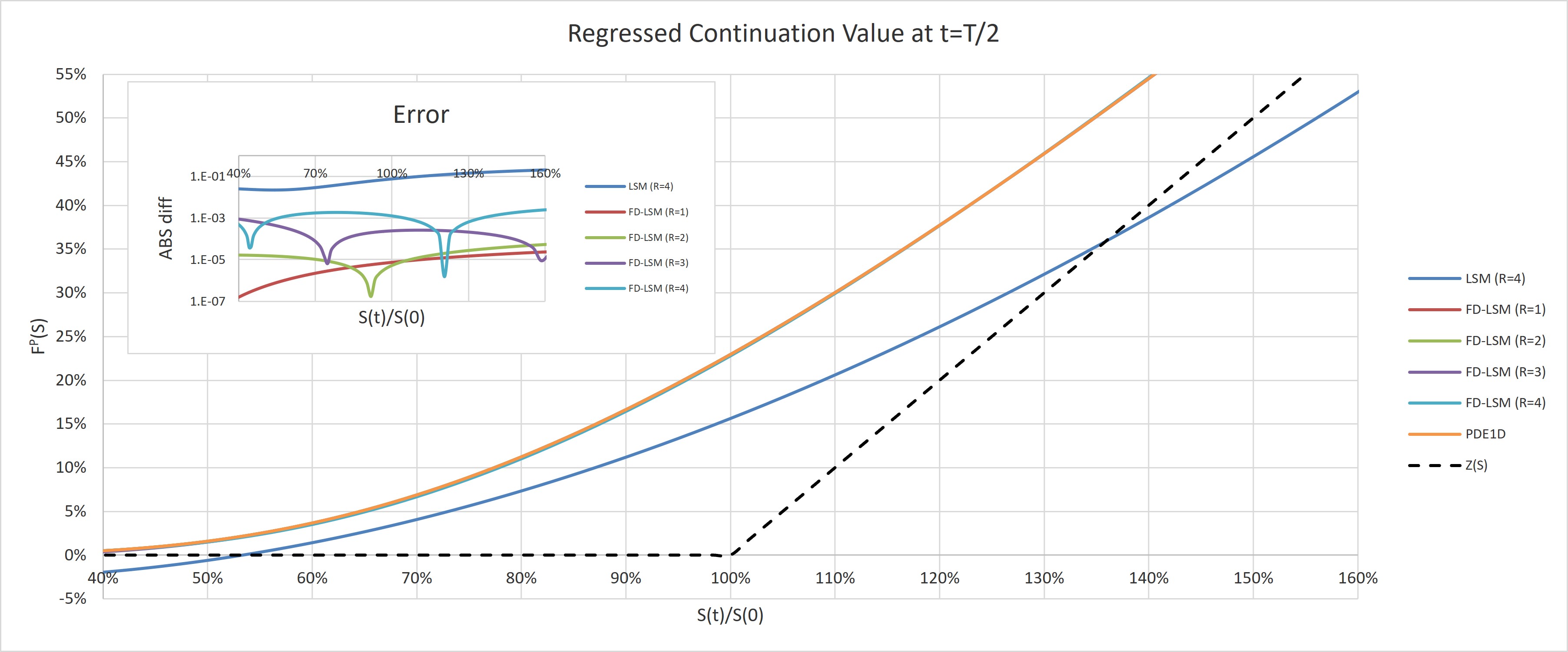
As a further examination on the stability of the regression method, we show the with arbitrary cutoff in Fig.3.2. Moving from low number of to medium level, e.g., , we can see a significant improvement in terms of accuracy in LSM, where the is more or less monotonically converging towards benchmark, largely and qualitatively consistent with previous literature (Frank J. Fabozzi, (2017)) focusing on put options, except the minor deterioration from to in the call option case; However, beyond , the results deviate clearly away from benchmark in the call case, which is a clear sign of overfitting. On the other hand, for FD-LSM, the PV error against benchmark is bounded at 50 bps even up to for the call case. Although in this example the new regression method is exhibiting amazing robustness against overfitting, it is inadvisable to perform linear regression with high order of monomial terms in practice. From now on, we restrict and cap the cutoff to 5, unless specified otherwise.


3.2 Bermudan Option with and under Black-Scholes
Next, we further look at the case of , where and . For a fair comparison between FD-LSM and LSM, we use the same number of regressors with fixed: LSM makes use of full monomials up to the cubic term, whereas FD-LSM only uses perturbational monomials up to the quadratic term, apart form the main FD regressor. Looking at PV results as seen in Tab.3.2, the maximum of difference in FD-LSM against FD PDE2D benchmark 777We use alternating direction implicit method (McKee & Mitchell, (1970)) in PDE2D. is merely 17 bps, whereas the counterpart in LSM is more than 2%, well beyond the simulation standard errors. Also, the computational overhead to achieve such accuracy is moderate as shown in the c.t. comparison. Last but not least, the Optimized Exercise Boundaries method (Opt-EB), as mentioned in Appendix A.4, can provide a valid independent check, although it tends to slightly underprice the option due to partial convergence in the external optimization.
Moving to , where , , and , The PV’s and c.t.’s under each various methods are shown in Tab.3.3. Different from low dimensions, full FD PDE result is no longer available; fortunately, we still have Opt-EB as an independent lower bound estimate.
Similar to lower dimensions, the new FD-LSM exhibits excellent agreement against benchmark consistently in terms of PV difference, outperforming traditional LSM for various put/call and settings: the maximum of differences between LSM and Opt-EB are 0.62% and 1.56% for put and call, respectively, and LSM underprices all test cases; whereas FD-LSM outperforms Opt-EB by up to 20 bps for put options and only underprices call options by 5 bps as maximum. For computational efficiency, as we can see from the c.t. columns between the two methods, the overhead due to additional PDE1D solver and cubic spline interpolation is insignificant.
| P/C | PDE2D | LSM (=4) | FD-LSM (=4) | Opt-EB | |||||||||
| PV | c.t. | PV | s.e. | Diff | c.t. | PV | s.e. | Diff | c.t. | PV | Diff | ||
| P | 90% | 17.94% | 0.5 | 17.02% | 0.07% | -0.91% | 2.5 | 17.94% | 0.07% | 0.01% | 2.8 | 17.85% | -0.09% |
| P | 50% | 15.59% | 0.4 | 14.81% | 0.06% | -0.77% | 2.6 | 15.56% | 0.06% | -0.03% | 2.8 | 15.48% | -0.11% |
| P | 10% | 13.06% | 0.4 | 12.42% | 0.05% | -0.64% | 2.5 | 13.05% | 0.05% | -0.01% | 2.7 | 12.92% | -0.14% |
| C | 90% | 33.35% | 0.4 | 31.22% | 0.19% | -2.13% | 2.4 | 33.17% | 0.23% | -0.17% | 2.7 | 33.32% | -0.03% |
| C | 50% | 31.10% | 0.5 | 29.10% | 0.17% | -2.00% | 2.5 | 30.98% | 0.21% | -0.12% | 2.9 | 31.08% | -0.02% |
| C | 10% | 28.72% | 0.5 | 26.98% | 0.15% | -1.74% | 2.6 | 28.56% | 0.18% | -0.16% | 2.9 | 28.71% | -0.01% |
| PC | Opt-EB | LSM (=4) | FD-LSM (=4) | |||||||
| PV | s.e. | Diff | c.t. | PV | s.e. | Diff | c.t. | |||
| P | 90% | 13.80% | 13.18% | 0.06% | -0.62% | 4.0 | 13.84% | 0.05% | 0.04% | 4.5 |
| P | 50% | 10.68% | 10.23% | 0.05% | -0.45% | 4.0 | 10.77% | 0.04% | 0.09% | 4.4 |
| P | 10% | 6.86% | 6.57% | 0.03% | -0.29% | 4.2 | 7.06% | 0.03% | 0.20% | 4.7 |
| C | 90% | 29.30% | 27.74% | 0.16% | -1.56% | 4.5 | 29.29% | 0.19% | -0.01% | 4.6 |
| C | 50% | 26.33% | 24.92% | 0.14% | -1.41% | 4.1 | 26.28% | 0.15% | -0.05% | 4.6 |
| C | 10% | 22.91% | 21.56% | 0.10% | -1.35% | 4.2 | 22.87% | 0.12% | -0.04% | 4.5 |
3.3 Bermudan Option with under Heston Stochastic Volatility
Here we consider Bermudan option pricing under Heston model as mentioned in Sec. 2.6.2. For Heston parameters, we use , , , , , and . We consider a monthly exercisable put option with and ; and are used in the simulation. In LSM, we use monomials regressors up to cubic terms, i.e., and in FD-LSM, up to quadratic terms are used. We compare LSM and FD-LSM with the method “LSMC-PDE” proposed by Farahany et al., (2020) using the same settings. As we can see in Tab. 3.4, both FD-LSM and LSMC-PDE are returning PVs closer to PDE2D benchmark than classical LSM.
One interesting observation is that LSMC-PDE seems to be biased high compared to the benchmark, whereas LSM and FD-LSM are biased low. As mentioned before, LSMC-PDE is essentially applying the least-squares estimator on the value function as an extension of Tsitsiklis & Van Roy, (2001), whereas LSM and FD-LSM apply the approximation in the stopping time determination only following Longstaff & Schwartz, (2001). Previous study by Stentoft, (2014) has concluded that the latter achieves a smaller absolute low bias with sub-optimality and less error accumulation compared to the former, based on a thorough comparison from both theoretical and numerical perspectives.
| LSM (cubic) | FD-LSM (quadratic) | LSMC-PDE | PDE2D | ||||||
| PV | s.e. | c.t. | PV | s.e. | c.t. | PV | s.e. | c.t. | PV |
| 14.41% | 0.03% | 2.9 | 14.49% | 0.03% | 3.0 | 14.53% | 0.01% | 7.0 | 14.51% |
3.4 EPE/CVA for European option in under Black-Scholes
In this section, we evaluate the performance of FD-LSM in the context of EPE/CVA calculation for European options. Assuming we (the party) are long an uncollateralized European call option issued by the counterparty, we apply the same market parameters as Sec.3.2 with . The option is struck at 100% with , and the EPE is evaluated with monthly discretized steps.
Since the portfolio has only one positive payoff to the party, it follows that its discounted option value under measure is a martingale, hence its expected value, i.e. EPE*, is constant over time:
where is the option PV that can be computed exactly with usual simulation approach as benchmark.
First, we inspect the EPE* profile, which is relevant to the CVA without considering WWR. In Fig.3.3, we plot the this profile using various cutoff under LSM and FD-LSM, where the s.e. is shown as error bar for indication. For LSM, EPE* deviates away from benchmark by up to 10 times of s.e. especially near the terminal end, with low level of ; by increasing , the discrepancy is reduced in the longer end; however, at the same time, in the short end, there are spikes with abnormally sizable error bar arising around for , indicting some kind of numerical instability.
On the other hand, for FD-LSM, we see very accurate agreement between calculated EPE* against theoretical benchmark for various in general. It is worth noticing that even with , the profile is much smoother with less angularities in terms of both frequency and intensity, than the LSM counterpart. Nevertheless, in both regression methods, the case with exhibits noticeable instability due to overfitting, as mentioned and shown in Bermuda option pricing previously; thus in practice, such high number of cutoff should be avoided for stability.


Now we continue to evaluate the total CVA using Eqn.2.12, taking into account WWR. As numerical settings, we use ; for the hazard rate, and are used, which are assumed to have been calibrated to counterparty credit spread using exact mark-to-market option values, and thus are independent of least-squares approximation. As seen in Tab. 3.5, as increases, CVA under LSM is exhibiting unstable move especially for , and the s.e. is showing explosive values up to 78 bps (). By contrast, FD-LSM generates much more stable CVA all the way up to very high cutoff with a maximum s.e. capped at 27 bps ().
| LSM | FD-LSM | |||
| CVA | s.e. | CVA | s.e. | |
| 3 | 2.30% | 0.01% | 2.27% | 0.01% |
| 4 | 2.28% | 0.01% | 2.27% | 0.01% |
| 5 | 2.27% | 0.01% | 2.27% | 0.01% |
| 6 | 2.27% | 0.01% | 2.27% | 0.01% |
| 7 | 2.27% | 0.01% | 2.27% | 0.01% |
| 8 | 2.29% | 0.03% | 2.28% | 0.02% |
| 9 | 2.36% | 0.10% | 2.36% | 0.10% |
| 10 | 2.52% | 0.26% | 2.37% | 0.11% |
| 11 | 3.71% | 0.78% | 2.54% | 0.27% |
In the context of EPE and CVA calculation, we not only further showcased the accuracy of FD-LSM over LSM, but also demonstrated the stability of the new method over time direction, i.e., time span between the regression variables and realized cash flows.
3.5 WIC from to under Black-Scholes and Local Volatility
As a finial numerical example, we will look at a WIC with 5-50 underlyings in the basket. For contractual parameters, we use coupon barrier , knock-in barrier and strike . Unless specified otherwise, underlying market data used are shown in Tab.3.6, where we consider both Black-Scholes and Local Volatility settings, respectively. In the simulation, we use and paths for regression and pricing, respectively, with weekly discretization steps.
| Stock tag with | |||||
| Dividend rate | 3% | 2% | 5% | 0% | 4% |
| Black-Scholes Volatility | 20% | 30% | 25% | 24% | 15% |
| Local Volatility | |||||
Black-Scholes setting: As presented in Tab.3.7, we show the PV and expected life between LSM and FD-LSM on WIC for various underlying market data and contractual parameters. In -th () rows of Tab.3.7 the same parameters as Liang et al., (2021) in their Tab. 5.5 are used and our LSM results are perfectly in-line888We do not suffer from any memory issues up to 50 dimension under x64 system as experienced by Liang et al., although FD-LSM gives marginally lower PV. However, in these cases, the coupon rate is too high, in particular compared to , and thus the issuer will almost surely call the product on 1-st exercise date as indicated by for . If we stress to in -th rows of Tab.3.7, the FD-LSM gives much lower PV than LSM by up to 3.3 times of s.e.. Moreover, if we change to , the difference ratio becomes 10+ as seen in -th rows, which is significant for a short dated option with few exercise dates. As a more comprehensive experiment to examine the accuracy of regression schemes, we use a much wider range of parameter sets by varying as well as the dimension (number of assets) in Tab.3.7. Since the optimal stopping strategy is a result of equilibrium due to competition among all these factors, with a wide range of parameter sets, it is expected to drive the change of exercise boundary, generating various testing scenarios. Going through all rows in Tab.3.7, FD-LSM always outperforms LSM by achieving a lower PV, and thus better results due to the nature of minimization problem using the same simulation paths, with difference ratio ranging from 0.2 to 28.8; and the outperformance is consistent from moderate () to high () dimensions. In practice, apart from achieving more accurate PV, we expect that the new method would naturally suppress the instability due to hopping between sub-optimal states in the scheme of bumping market factors and re-evaluation for greeks calculation.
| # | LSM (=4) | FD-LSM (=4) | c.t. Diff% | |||||||||||
| PV(%) | s.e.(%) | PV(%) | s.e.(%) | |||||||||||
| 1 | 5 | 30% | 1 | 4 | 20% | 1% | 104.43 | 0.01 | 0.29 | 104.43 | 0.01 | 0.29 | 0.4 | 8% |
| 2 | 5 | 30% | 1 | 4 | 1% | 1% | 98.57 | 0.02 | 0.80 | 98.49 | 0.02 | 0.99 | 3.3 | 5% |
| 3 | 5 | 90% | 1 | 4 | 1% | 5% | 95.56 | 0.02 | 0.96 | 95.39 | 0.02 | 1.01 | 10.3 | 6% |
| 4 | 5 | 30% | 5 | 4 | 1% | 5% | 63.59 | 0.07 | 4.79 | 62.88 | 0.07 | 5.00 | 10.2 | 2% |
| 5 | 5 | 90% | 5 | 4 | 1% | 5% | 71.33 | 0.06 | 4.64 | 70.16 | 0.06 | 5.00 | 18.8 | 5% |
| 6 | 5 | 30% | 10 | 4 | 1% | 5% | 41.30 | 0.07 | 9.76 | 40.65 | 0.06 | 10.01 | 9.8 | 3% |
| 7 | 5 | 90% | 10 | 4 | 1% | 5% | 51.80 | 0.07 | 9.43 | 50.30 | 0.06 | 10.01 | 22.7 | 4% |
| 8 | 5 | 30% | 1 | 12 | 20% | 1% | 101.54 | 0.01 | 0.13 | 101.52 | 0.01 | 0.14 | 1.7 | 5% |
| 9 | 5 | 30% | 1 | 12 | 1% | 1% | 98.17 | 0.02 | 0.82 | 98.01 | 0.02 | 1.01 | 6.9 | 6% |
| 10 | 5 | 90% | 1 | 12 | 1% | 5% | 95.11 | 0.02 | 0.95 | 94.89 | 0.02 | 1.01 | 13.7 | 6% |
| 11 | 5 | 30% | 5 | 12 | 1% | 5% | 62.06 | 0.07 | 4.81 | 61.35 | 0.07 | 5.00 | 10.4 | 4% |
| 12 | 5 | 90% | 5 | 12 | 1% | 5% | 69.39 | 0.06 | 4.67 | 68.16 | 0.06 | 5.00 | 20.3 | 4% |
| 13 | 5 | 30% | 10 | 12 | 1% | 5% | 39.16 | 0.06 | 9.78 | 38.46 | 0.06 | 10.00 | 11.0 | 6% |
| 14 | 5 | 90% | 10 | 12 | 1% | 5% | 48.74 | 0.06 | 9.47 | 47.15 | 0.06 | 10.01 | 25.3 | 4% |
| 15 | 10 | 30% | 1 | 4 | 20% | 1% | 103.93 | 0.02 | 0.35 | 103.92 | 0.02 | 0.35 | 0.6 | 6% |
| 16 | 10 | 30% | 1 | 4 | 1% | 1% | 97.32 | 0.03 | 0.89 | 97.24 | 0.03 | 0.98 | 2.5 | 4% |
| 17 | 10 | 90% | 1 | 4 | 1% | 5% | 95.34 | 0.02 | 0.94 | 95.09 | 0.02 | 1.01 | 12.9 | 4% |
| 18 | 10 | 30% | 5 | 4 | 1% | 5% | 54.31 | 0.07 | 4.85 | 53.84 | 0.07 | 4.98 | 6.3 | 4% |
| 19 | 10 | 90% | 5 | 4 | 1% | 5% | 68.77 | 0.07 | 4.68 | 67.71 | 0.06 | 5.00 | 16.0 | 3% |
| 20 | 10 | 30% | 10 | 4 | 1% | 5% | 31.68 | 0.06 | 9.88 | 31.36 | 0.06 | 9.98 | 5.2 | 4% |
| 21 | 10 | 90% | 10 | 4 | 1% | 5% | 48.67 | 0.07 | 9.50 | 47.37 | 0.06 | 10.01 | 19.1 | 2% |
| 22 | 10 | 30% | 1 | 12 | 20% | 1% | 101.58 | 0.01 | 0.10 | 101.58 | 0.01 | 0.09 | 0.2 | 9% |
| 23 | 10 | 30% | 1 | 12 | 1% | 1% | 97.46 | 0.03 | 0.76 | 97.29 | 0.03 | 0.86 | 5.4 | 7% |
| 24 | 10 | 90% | 1 | 12 | 1% | 5% | 95.69 | 0.02 | 0.86 | 95.12 | 0.02 | 1.01 | 28.8 | 7% |
| 25 | 10 | 30% | 5 | 12 | 1% | 5% | 54.61 | 0.07 | 4.80 | 53.95 | 0.07 | 4.96 | 8.8 | 5% |
| 26 | 10 | 90% | 5 | 12 | 1% | 5% | 69.27 | 0.07 | 4.55 | 67.77 | 0.06 | 5.00 | 22.3 | 4% |
| 27 | 10 | 30% | 10 | 12 | 1% | 5% | 31.92 | 0.06 | 9.84 | 31.49 | 0.06 | 9.98 | 7.0 | 7% |
| 28 | 10 | 90% | 10 | 12 | 1% | 5% | 49.22 | 0.07 | 9.36 | 47.50 | 0.06 | 10.01 | 24.8 | 3% |
| 29 | 20 | 30% | 1 | 4 | 20% | 1% | 102.43 | 0.04 | 0.50 | 102.42 | 0.04 | 0.50 | 0.2 | 5% |
| 30 | 20 | 30% | 1 | 4 | 1% | 1% | 95.13 | 0.04 | 0.92 | 95.07 | 0.04 | 0.94 | 1.3 | 4% |
| 31 | 20 | 90% | 1 | 4 | 1% | 5% | 95.00 | 0.02 | 0.94 | 94.73 | 0.02 | 1.01 | 11.8 | 2% |
| 32 | 20 | 30% | 5 | 4 | 1% | 5% | 44.53 | 0.07 | 4.93 | 44.35 | 0.07 | 4.98 | 2.5 | 5% |
| 33 | 20 | 90% | 5 | 4 | 1% | 5% | 66.17 | 0.07 | 4.73 | 65.30 | 0.07 | 5.00 | 12.5 | 3% |
| 34 | 20 | 30% | 10 | 4 | 1% | 5% | 23.45 | 0.05 | 9.96 | 23.39 | 0.05 | 9.98 | 1.3 | 1% |
| 35 | 20 | 90% | 10 | 4 | 1% | 5% | 45.66 | 0.07 | 9.62 | 44.66 | 0.07 | 10.01 | 14.4 | 4% |
| 36 | 20 | 30% | 1 | 12 | 20% | 1% | 101.31 | 0.02 | 0.17 | 101.29 | 0.02 | 0.17 | 0.9 | 7% |
| 37 | 20 | 30% | 1 | 12 | 1% | 1% | 95.29 | 0.04 | 0.84 | 95.20 | 0.04 | 0.87 | 2.1 | 3% |
| 38 | 20 | 90% | 1 | 12 | 1% | 5% | 95.39 | 0.02 | 0.85 | 94.77 | 0.02 | 1.01 | 27.2 | 4% |
| 39 | 20 | 30% | 5 | 12 | 1% | 5% | 44.79 | 0.07 | 4.90 | 44.48 | 0.07 | 4.96 | 4.3 | 4% |
| 40 | 20 | 90% | 5 | 12 | 1% | 5% | 66.64 | 0.07 | 4.62 | 65.38 | 0.07 | 5.00 | 17.9 | 6% |
| 41 | 20 | 30% | 10 | 12 | 1% | 5% | 23.63 | 0.05 | 9.95 | 23.55 | 0.05 | 9.97 | 1.6 | 2% |
| 42 | 20 | 90% | 10 | 12 | 1% | 5% | 45.99 | 0.07 | 9.54 | 44.76 | 0.07 | 10.01 | 17.6 | 7% |
| 43 | 50 | 30% | 1 | 4 | 20% | 1% | 97.62 | 0.06 | 0.74 | 97.59 | 0.06 | 0.76 | 0.4 | 4% |
| 44 | 50 | 30% | 1 | 4 | 1% | 1% | 90.43 | 0.06 | 0.92 | 90.37 | 0.06 | 0.95 | 1.1 | 3% |
| 45 | 50 | 90% | 1 | 4 | 1% | 5% | 94.51 | 0.03 | 0.93 | 94.21 | 0.03 | 1.01 | 11.2 | 4% |
| 46 | 50 | 30% | 5 | 4 | 1% | 5% | 33.34 | 0.06 | 4.98 | 33.31 | 0.06 | 4.99 | 0.5 | 1% |
| 47 | 50 | 90% | 5 | 4 | 1% | 5% | 62.91 | 0.07 | 4.80 | 62.26 | 0.07 | 5.00 | 8.9 | 3% |
| 48 | 50 | 30% | 10 | 4 | 1% | 5% | 16.09 | 0.03 | 10.00 | 16.08 | 0.03 | 10.00 | 0.4 | 2% |
| 49 | 50 | 90% | 10 | 4 | 1% | 5% | 42.03 | 0.07 | 9.75 | 41.39 | 0.07 | 10.01 | 9.4 | 2% |
| 50 | 50 | 30% | 1 | 12 | 20% | 1% | 98.25 | 0.05 | 0.60 | 98.23 | 0.05 | 0.61 | 0.3 | 4% |
| 51 | 50 | 30% | 1 | 12 | 1% | 1% | 90.65 | 0.06 | 0.87 | 90.54 | 0.06 | 0.91 | 1.9 | 5% |
| 52 | 50 | 90% | 1 | 12 | 1% | 5% | 94.84 | 0.03 | 0.85 | 94.22 | 0.03 | 1.01 | 23.0 | 4% |
| 53 | 50 | 30% | 5 | 12 | 1% | 5% | 33.52 | 0.06 | 4.97 | 33.43 | 0.06 | 4.98 | 1.5 | 1% |
| 54 | 50 | 90% | 5 | 12 | 1% | 5% | 63.43 | 0.07 | 4.68 | 62.35 | 0.07 | 5.00 | 14.5 | 3% |
| 55 | 50 | 30% | 10 | 12 | 1% | 5% | 16.21 | 0.04 | 9.99 | 16.17 | 0.03 | 10.00 | 0.9 | 3% |
| 56 | 50 | 90% | 10 | 12 | 1% | 5% | 42.48 | 0.07 | 9.63 | 41.49 | 0.07 | 10.01 | 14.0 | 3% |
Finally, we also check the calculation time in last column of Tab. 3.7. In general, there is expected mild deterioration when switching to the new method, contributed by the additional PDE1D solvers and the cubic spline interpolation. However, the relative impacts are merely in single-digit range; thus we don’t expect this amount of impact would become a “showstopper” when applying the new regression scheme for generic option pricing and risk management from practitioners’ point of view.
| # | LSM (=4) | FD-LSM (=4) | c.t. Diff% | |||||||||||
| PV(%) | s.e.(%) | PV(%) | s.e.(%) | |||||||||||
| 1 | 5 | 30% | 1 | 4 | 20% | 1% | 104.77 | 0.00 | 0.26 | 104.77 | 0.00 | 0.29 | 0.0 | 6% |
| 2 | 5 | 30% | 1 | 4 | 1% | 1% | 99.84 | 0.01 | 0.64 | 99.81 | 0.01 | 0.99 | 3.6 | 9% |
| 3 | 5 | 90% | 1 | 4 | 1% | 5% | 96.06 | 0.01 | 1.01 | 96.05 | 0.01 | 1.01 | 0.3 | 6% |
| 4 | 5 | 30% | 5 | 4 | 1% | 5% | 72.15 | 0.06 | 4.79 | 71.47 | 0.06 | 5.00 | 11.4 | 10% |
| 5 | 5 | 90% | 5 | 4 | 1% | 5% | 76.55 | 0.05 | 4.68 | 75.52 | 0.05 | 5.00 | 20.4 | 10% |
| 6 | 5 | 30% | 10 | 4 | 1% | 5% | 46.58 | 0.07 | 9.76 | 45.94 | 0.07 | 10.01 | 9.6 | 4% |
| 7 | 5 | 90% | 10 | 4 | 1% | 5% | 55.37 | 0.06 | 9.46 | 53.97 | 0.06 | 10.01 | 22.1 | 10% |
| 8 | 5 | 30% | 1 | 12 | 20% | 1% | 101.43 | 0.00 | 0.26 | 101.43 | 0.00 | 0.14 | 0.0 | 9% |
| 9 | 5 | 30% | 1 | 12 | 1% | 1% | 99.33 | 0.01 | 0.81 | 99.24 | 0.01 | 1.01 | 11.2 | 0% |
| 10 | 5 | 90% | 1 | 12 | 1% | 5% | 95.58 | 0.01 | 0.98 | 95.50 | 0.01 | 1.01 | 15.9 | 3% |
| 11 | 5 | 30% | 5 | 12 | 1% | 5% | 70.49 | 0.06 | 4.67 | 69.27 | 0.06 | 5.00 | 20.7 | 11% |
| 12 | 5 | 90% | 5 | 12 | 1% | 5% | 74.57 | 0.05 | 4.58 | 73.02 | 0.05 | 5.00 | 31.1 | 2% |
| 13 | 5 | 30% | 10 | 12 | 1% | 5% | 43.76 | 0.07 | 9.68 | 42.78 | 0.06 | 10.00 | 15.0 | 8% |
| 14 | 5 | 90% | 10 | 12 | 1% | 5% | 52.01 | 0.06 | 9.34 | 50.01 | 0.06 | 10.01 | 32.6 | 9% |
| 15 | 10 | 30% | 1 | 4 | 20% | 1% | 104.76 | 0.00 | 0.35 | 104.76 | 0.00 | 0.35 | 0.0 | 3% |
| 16 | 10 | 30% | 1 | 4 | 1% | 1% | 99.61 | 0.01 | 0.89 | 99.59 | 0.01 | 0.98 | 1.6 | 2% |
| 17 | 10 | 90% | 1 | 4 | 1% | 5% | 96.01 | 0.01 | 0.94 | 96.01 | 0.01 | 1.01 | 0.7 | 7% |
| 18 | 10 | 30% | 5 | 4 | 1% | 5% | 65.27 | 0.07 | 4.85 | 64.72 | 0.07 | 4.98 | 7.7 | 1% |
| 19 | 10 | 90% | 5 | 4 | 1% | 5% | 74.83 | 0.06 | 4.68 | 73.82 | 0.05 | 5.00 | 18.2 | 2% |
| 20 | 10 | 30% | 10 | 4 | 1% | 5% | 36.82 | 0.07 | 9.88 | 36.53 | 0.07 | 9.98 | 4.3 | 3% |
| 21 | 10 | 90% | 10 | 4 | 1% | 5% | 52.44 | 0.07 | 9.50 | 51.15 | 0.06 | 10.01 | 19.3 | 2% |
| 22 | 10 | 30% | 1 | 12 | 20% | 1% | 101.61 | 0.00 | 0.10 | 101.61 | 0.00 | 0.09 | 0.0 | 8% |
| 23 | 10 | 30% | 1 | 12 | 1% | 1% | 99.65 | 0.01 | 0.76 | 99.63 | 0.01 | 0.86 | 2.0 | 6% |
| 24 | 10 | 90% | 1 | 12 | 1% | 5% | 96.12 | 0.01 | 0.86 | 96.02 | 0.01 | 1.01 | 14.5 | 8% |
| 25 | 10 | 30% | 5 | 12 | 1% | 5% | 65.77 | 0.07 | 4.80 | 64.87 | 0.07 | 4.96 | 12.8 | 5% |
| 26 | 10 | 90% | 5 | 12 | 1% | 5% | 75.33 | 0.06 | 4.55 | 73.85 | 0.05 | 5.00 | 26.3 | 4% |
| 27 | 10 | 30% | 10 | 12 | 1% | 5% | 37.13 | 0.07 | 9.84 | 36.68 | 0.07 | 9.98 | 6.7 | 12% |
| 28 | 10 | 90% | 10 | 12 | 1% | 5% | 52.93 | 0.07 | 9.36 | 51.25 | 0.06 | 10.01 | 24.9 | 1% |
| 29 | 20 | 30% | 1 | 4 | 20% | 1% | 104.75 | 0.00 | 0.26 | 104.75 | 0.00 | 0.26 | 0.0 | 5% |
| 30 | 20 | 30% | 1 | 4 | 1% | 1% | 99.24 | 0.02 | 0.82 | 99.23 | 0.02 | 0.82 | 0.9 | 5% |
| 31 | 20 | 90% | 1 | 4 | 1% | 5% | 95.93 | 0.01 | 1.00 | 95.93 | 0.01 | 1.01 | 1.0 | 2% |
| 32 | 20 | 30% | 5 | 4 | 1% | 5% | 56.70 | 0.08 | 4.88 | 56.38 | 0.08 | 4.96 | 4.2 | 2% |
| 33 | 20 | 90% | 5 | 4 | 1% | 5% | 72.77 | 0.06 | 4.76 | 72.00 | 0.06 | 5.00 | 12.8 | 2% |
| 34 | 20 | 30% | 10 | 4 | 1% | 5% | 27.62 | 0.06 | 9.95 | 27.50 | 0.06 | 9.99 | 2.0 | 4% |
| 35 | 20 | 90% | 10 | 4 | 1% | 5% | 49.60 | 0.07 | 9.59 | 48.51 | 0.07 | 10.01 | 15.8 | 1% |
| 36 | 20 | 30% | 1 | 12 | 20% | 1% | 101.61 | 0.00 | 0.08 | 101.61 | 0.01 | 0.08 | 0.0 | 7% |
| 37 | 20 | 30% | 1 | 12 | 1% | 1% | 99.34 | 0.02 | 0.56 | 99.30 | 0.02 | 0.68 | 2.5 | 5% |
| 38 | 20 | 90% | 1 | 12 | 1% | 5% | 96.14 | 0.01 | 0.95 | 95.94 | 0.01 | 1.01 | 22.6 | 4% |
| 39 | 20 | 30% | 5 | 12 | 1% | 5% | 57.06 | 0.08 | 4.81 | 56.53 | 0.08 | 4.93 | 6.9 | 2% |
| 40 | 20 | 90% | 5 | 12 | 1% | 5% | 73.48 | 0.06 | 4.56 | 72.06 | 0.06 | 5.00 | 23.3 | 3% |
| 41 | 20 | 30% | 10 | 12 | 1% | 5% | 27.86 | 0.06 | 9.92 | 27.65 | 0.06 | 9.98 | 3.6 | 6% |
| 42 | 20 | 90% | 10 | 12 | 1% | 5% | 49.99 | 0.07 | 9.49 | 48.62 | 0.07 | 10.01 | 19.7 | 6% |
| 43 | 50 | 30% | 1 | 4 | 20% | 1% | 104.66 | 0.01 | 0.28 | 104.66 | 0.01 | 0.28 | 0.0 | 2% |
| 44 | 50 | 30% | 1 | 4 | 1% | 1% | 98.18 | 0.03 | 0.88 | 98.16 | 0.03 | 0.89 | 0.8 | 4% |
| 45 | 50 | 90% | 1 | 4 | 1% | 5% | 95.84 | 0.01 | 1.00 | 95.83 | 0.01 | 1.01 | 0.6 | 1% |
| 46 | 50 | 30% | 5 | 4 | 1% | 5% | 43.95 | 0.08 | 4.96 | 43.88 | 0.08 | 4.98 | 0.9 | 0% |
| 47 | 50 | 90% | 5 | 4 | 1% | 5% | 70.30 | 0.07 | 4.77 | 69.58 | 0.06 | 5.00 | 11.1 | 1% |
| 48 | 50 | 30% | 10 | 4 | 1% | 5% | 18.30 | 0.04 | 9.99 | 18.27 | 0.04 | 10.00 | 0.6 | 4% |
| 49 | 50 | 90% | 10 | 4 | 1% | 5% | 46.08 | 0.07 | 9.72 | 45.37 | 0.07 | 10.01 | 10.2 | 1% |
| 50 | 50 | 30% | 1 | 12 | 20% | 1% | 101.61 | 0.00 | 0.08 | 101.61 | 0.00 | 0.08 | 0.0 | 3% |
| 51 | 50 | 30% | 1 | 12 | 1% | 1% | 98.31 | 0.03 | 0.69 | 98.22 | 0.03 | 0.77 | 3.4 | 3% |
| 52 | 50 | 90% | 1 | 12 | 1% | 5% | 96.06 | 0.01 | 0.95 | 95.85 | 0.01 | 1.01 | 19.9 | 3% |
| 53 | 50 | 30% | 5 | 12 | 1% | 5% | 44.29 | 0.08 | 4.91 | 44.07 | 0.08 | 4.95 | 2.9 | 2% |
| 54 | 50 | 90% | 5 | 12 | 1% | 5% | 70.94 | 0.07 | 4.60 | 69.66 | 0.06 | 5.00 | 19.4 | 4% |
| 55 | 50 | 30% | 10 | 12 | 1% | 5% | 18.44 | 0.04 | 9.98 | 18.40 | 0.04 | 9.99 | 1.0 | 8% |
| 56 | 50 | 90% | 10 | 12 | 1% | 5% | 46.53 | 0.07 | 9.59 | 45.46 | 0.07 | 10.01 | 15.1 | 2% |
Local Volatility setting: We repeat previous numerical experiment under a local volatility setting with
This hypothetical functional form can generate a steep skew to mimic a stressed market condition. The results are presented in Tab.3.8. We observe that in all test scenarios, FD-LSM outperforms LSM, with a maximum PV difference ratio reaching 32.6, compared to 28.8 under constant volatilities. In terms of calculation time, mild relative impacts are observed too. Therefore, we can conclude that FD-LSM is performing well even under a general multi-variate local volatility setting.
4 Conclusion
In this manuscript, we presented a novel regression based approach for American-style option pricing. The formulism is to construct the ansatz to be regressed on using the 1D FD solution obtained from a backward PDE solver. Theoretical model-independent analysis indicates that the most effective least-square error reduction can be obtained by choosing a 1D payoff process with highest correlation against the original one. Effective dimension reduction methodologies to arrive at the 1D auxiliary process have also been discussed throughout various model settings, ranging from local volatility, to stochastic volatility (Heston model). Under this wide range of processes, numerical tests on Bermudan options and WIC indicate that FD-LSM produces accurate option prices benchmarking against FD-based full PDE approach in low dimensions (), and consistently overshadows classical LSM under high dimensions (up to 50). By stressing the market and contractual parameters, we showed that the combination of the ad-hoc FD-based ansatz and perturbational monomials as regressors, gives rise to stable results especially with exercise frontiers far away from the ATM region. At the same time, there has not been noticeable degradation in terms of the computational efficiency with the additional calculation in PDE solver and spline interpolation. This effective and efficient method can be implemented as a generic framework for pricing and risk management on structure derivative products with American-style exercise features. Going beyond option pricing, since LSM is also widely used to approximate the future exposure for products that cannot be valued analytically in the context of XVA, the new method is applicable there for the sake of accuracy and numerical stability.
Acknowledgments
The author would like to thank his team members and fellow quants for stimulating discussions on the subject and is particularly grateful to Andrei N. Soklakov. The author reports no conflicts of interest. The author alone is responsible for the content and writing of the paper. The views expressed in this article are those of the author alone and do not necessarily represent those of Citigroup. All errors are the author’s responsibility.
Appendix
A.1 Bermudan option
A Bermudan option is an American-style option that is written on the spot price of a basket , expressed as a weighted average of individual assets. Note that for mono-underlying structure, is just simply , where we ignore the subscript. It is exercisable by the holder on .
The exercise payoff is given by
The state variables can be reduced to as the only explanatory independent variable, considering the functional dependence of the payoff . Here is the strike price of the option.
Finally, is given by
A.2 Worst Of Issuer Callable Note
The worst of issuer callable note (WIC) is one of the most popular yield enhancement products in retail structured note market. On one hand, the investment performance of this product is capped by a equity dependent coupon rate; one the other hand, the issuer has the right to call the product with a return of principal, at his or her discretion, on exercise dates on or before maturity , i.e., the exercisability is on the issuer side. The performance is liked to a worst-of function on underlying assets .
There are a series of equity-dependent coupons announced on record dates in-line exactly with early exercise dates , and the coupon payments are in digital form with amount subjected to a coupon barrier :
where is annualized coupon rate per unit notional and is the annual coupon frequency, as well as the exercise frequency; the Heaviside step function is denoted by .
At maturity only, which is also the last coupon announcement date, there is a return of principal, as well as a short put option striking at with knocked-in barrier embedded:
where we have assumed the notional of the WIC is 1 for simplicity.
Different from a simple Bermudan option discussed previously, WIC is a much more complex product. There are several competing driving factors for the optimal stopping strategy to achieve a minimization of PV:
-
•
On the upside, there are digital coupons whose amounts are linked to underlying asset performance.
-
•
On the downside, the chance of being knocked in as a put option is against early termination by issuer.
-
•
The interest rate is also playing a vital role as it impacts the PV of the returned principal.
It is expected to pose much more challenge on the numerical approach in terms of accuracy of derivative pricing, due to presence of discontinuity (e.g. the knocked-in and coupon digital barrier) in the payoff.
In this problem, the worst of performance is the explanatory variable , which is the only driver for both the coupon performance and value of the knock in put option. Mathematically, the exercise payoff and option value are given by
and
respectively.
A.3 Regression Approach in Monte Carlo framework
The objective function to be minimized is the expected squared error in Eqn.2.7 w.r.t. the coefficients is
Translating this into the language within Monte Carlo framework, we have
where the superscript indicates that the variable is under of total regression Monte Carlo paths.
After some algebra, the minimization problem is equivalent to solving the linear system:
| (4.1) |
where the matrix and are defined as:
and
respectively.
A.4 Optimized Exercise Boundaries (Opt-EB)
As alternative independent check for the PV of American-style options, we introduce a brute force method within simulation framework. For ease of illustration but without loss of generality, we focus on Bermudan option only, although this method will work as expected given the payoff is monotonic.
First of all, we define the variational stopping time , in light of Eqn.2.10, as
which depends on defining the exercise boundaries on all exercise dates.
For a given , the European-style option PV can be obtained by standard Monte Carlo method with ease as .
Then the Bermudan option PV under Opt-EB can be computed via external optimization:
| (4.2) |
In practice, the result is obtain by optimizing the exercise boundary levels to achieve a maximum as much as possible999In our implementation, a multi-dimensional Simplex algorithm is used..
This brute-force variational method is a very time consuming approach, which can take many (up to 100+) iterations before achieving convergent results. However, it would be serving as one of few available benchmarks, or at lease lower (upper) bound estimates for holder (issuer) exercise, especially when full PDE FD solution is unavailable under higher dimensions with .
References
- Areal & Armada, (2008) Areal, N., Rodrigues A., & Armada, M.R. 2008. On improving the least squares Monte Carlo option valuation method. Review of Derivatives Research, 11, 119–151.
- Avellaneda & Boyer-Olson, (2002) Avellaneda, Marco, & Boyer-Olson, Dash. 2002. Reconstruction of Volatility: Pricing Index Options by the Steepest Descent Approximation. SSRN.
- Barraquand & Martineau, (1995) Barraquand, J., & Martineau, D. 1995. Numerical valuation of high dimensional multivariate american securities. The Journal of Financial and Quantitative Analysis, 30(3), 342–351.
- Boire et al., (2022) Boire, Francois-Michel, Reesor, R. Mark, & Stentoft, Lars. 2022. Bias Correction in the Least-Squares Monte Carlo Algorithm. SSRN.
- Broadie & Glasserman, (2004) Broadie, M., & Glasserman, P. 2004. A stochastic mesh method for pricing high-dimensional american options. Journal of Computational Finance, 7(4), 35–72.
- Clément et al., (2002) Clément, Emmanuelle, Lamberton, Damien, & Protter, Philip. 2002. An analysis of a least squares regression method for American option pricing. Finance and stochastics, 6, 449–471.
- Fabozzi et al., (2017) Fabozzi, Frank J, Paletta, Tommaso, & Tunaru, Radu. 2017. An improved least squares Monte Carlo valuation method based on heteroscedasticity. European Journal of Operational Research, 263(2), 698–706.
- Farahany et al., (2020) Farahany, David, Jackson, Kenneth R, & Jaimungal, Sebastian. 2020. Mixing LSMC and PDE methods to price Bermudan options. SIAM Journal on Financial Mathematics, 11(1), 201–239.
- Frank J. Fabozzi, (2017) Frank J. Fabozzi, Tommaso Paletta, Radu Tunaru. 2017. An improved least squares Monte Carlo valuation method based on heteroscedasticity. European Journal of Operational Research, 263(2), 698–706.
- Fujii & Takahashi, (2019) Fujii, M., Takahashi A., & Takahashi, M. 2019. Asymptotic expansion as prior knowledge in deep learning method for high dimensional BSDEs. Asia-Pacific Financial Markets, 26(3), 391–408.
- Gao et al., (2023) Gao, Chengfan, Gao, Siping, Hu, Ruimeng, & Zhu, Zimu. 2023. Convergence of the backward deep BSDE method with applications to optimal stopping problems. SIAM Journal on Financial Mathematics, 14(4), 1290–1303.
- Glasserman, (2004) Glasserman, Paul. 2004. Monte Carlo methods in financial engineering. Vol. 53. Springer.
- Gyöngy, (1986) Gyöngy, István. 1986. Mimicking the one-dimensional marginal distributions of processes having an Itô differential. Probability theory and related fields, 71(4), 501–516.
- Han et al., (2018) Han, Jiequn, Jentzen, Arnulf, & E, Weinan. 2018. Solving high-dimensional partial differential equations using deep learning. Proceedings of the National Academy of Sciences, 115(34), 8505–8510.
- Hull & White, (2012) Hull, John, & White, Alan. 2012. CVA and wrong-way risk. Financial Analysts Journal, 68(5), 58–69.
- Joshi & Kwon, (2016) Joshi, Mark, & Kwon, Oh Kang. 2016. Least Squares Monte Carlo Credit Value Adjustment with Small and Unidirectional Bias. International Journal of Theoretical and Applied Finance, 19(08), 1650048.
- Liang et al., (2021) Liang, Jian, Xu, Zhe, & Li, Peter. 2021. Deep learning-based least squares forward-backward stochastic differential equation solver for high-dimensional derivative pricing. Quantitative Finance, 21(8), 1309–1323.
- Longstaff & Schwartz, (2001) Longstaff, F., & Schwartz, E. 2001. Valuing American options by simulation: a simple least-squares approach. The Review of Financial Studies, 14(1), 113–147.
- McKee & Mitchell, (1970) McKee, S., & Mitchell, A. R. 1970. Alternating direction methods for parabolic equations in two space dimensions with a mixed derivative. The Computer Journal, 13(1), 81–86.
- Moreno, (2003) Moreno, M., Navas J.F. 2003. On the Robustness of Least-Squares Monte Carlo (LSM) for Pricing American Derivatives. Review of Derivatives Research, 6, 107–128.
- Søndergaard Rasmussen, (2002) Søndergaard Rasmussen, Nicki. 2002. Efficient Control Variates for Monte-Carlo Valuation of American Options. SSRN.
- Stentoft, (2001) Stentoft, L. 2001. Assessing the least squares Monte-Carlo approach to American option valuation. Review of Derivatives Research, 7(2), 129–168.
- Stentoft, (2014) Stentoft, Lars. 2014. Value function approximation or stopping time approximation: A comparison of two recent numerical methods for American option pricing using simulation and regression. Journal of Computational Finance, 18(1).
- Tian & Burrage, (2003) Tian, Tianhai, & Burrage, Kevin. 2003. Accuracy issues of Monte-Carlo methods for valuing American options. ANZIAM J., 44(C), 739–758.
- Tsitsiklis & Van Roy, (2001) Tsitsiklis, John N, & Van Roy, Benjamin. 2001. Regression methods for pricing complex American-style options. IEEE Transactions on Neural Networks, 12(4), 694–703.
- Woo et al., (2024) Woo, Jeechul, Liu, Chenru, & Choi, Jaehyuk. 2024. Leave-one-out least squares Monte Carlo algorithm for pricing Bermudan options. Journal of Futures Markets, 44(8), 1404–1428.