Fine Boundary–Layer structure in Linear Transport Theory

The linear transport equation provides a general model for neutral particle transport, including e.g. Neutron Transport and Radiative Transfer of photons, which impacts upon a wide range of disciplines in science and technology [1, 2, 3, 4, 5]. In this context, this paper identifies and characterizes a significant boundary–layer structure which, albeit present in e.g. eigenfunction systems for one dimensional problems [6, Ch. 4] (as they must be in view of the theoretical discussion presented in this paper), has not previously been correctly accounted for or even fully recognized, namely, a structure of sharp solution transitions with unbounded gradients arbitrarily close to interface boundaries.

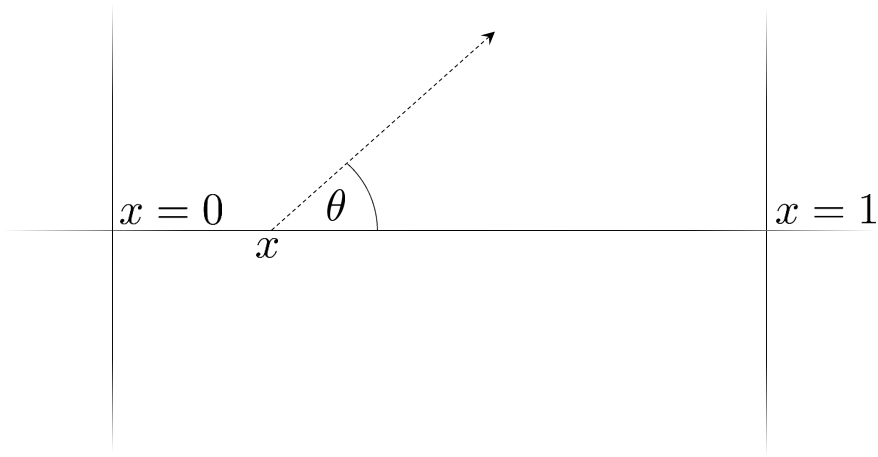
The equation for time–independent neutral particle transport in a one–dimensional plane–parallel geometry (Fig. 1), with isotropic scattering and Fresnel boundary conditions, is given by

$$\begin{split}&\xi\frac{\partial}{\partial x}u(x,\xi)+\mu_{t}(x)u(x,\xi)=\\ &\qquad\;\;\;\;\;\frac{\mu_{s}(x)}{2}\int_{-1}^{1}u(x,\xi^{\prime})d\xi^{\prime}+q(x,\xi),\\ &u(x=0,\xi)=\mathcal{R}(\xi)u(x=0,\xi_{R})\;\forall\xi>0,\\ &u(x=1,\xi)=\mathcal{R}(\xi)u(x=1,\xi_{R})\;\forall\xi<0.\end{split}$$

(1)

Here $\xi=\cos(\theta)$, and, letting $\mu_{s}(x)$ and $\mu_{a}(x)$ denote the macroscopic scattering and absorption coefficients, respectively, the total transport coefficient is $\mu_{t}(x)=\mu_{a}(x)+\mu_{s}(x)$. The integral term accounts for the angular redistribution of particles due to scattering, $q(x,\xi)$ is an external source, and the Fresnel boundary conditions model the reflection of particles at the boundary interface due to refractive-index differences—wherein $\xi_{R}=-\xi$ equals the reflected direction cosine and $\mathcal{R}(\xi)$ the corresponding Fresnel reflection coefficient [7].

Noting that the coefficient $\xi$ of the highest order derivative in (1) tends to zero as $\theta\to\pi/2$, the existence of sharp spatial gradients in the solution $u(x,\xi)$ for such angles and for $x$ near the interfaces $x=0$ and $x=1$ may be expected [8, Ch. 9], leading to unbounded spatial gradients at points $(x,\xi)$ near $(0,0)$ and $(1,0)$. Such “boundary–layer” structures, which are caused by the existence of a spatial boundary condition in conjunction with a vanishingly small coefficient for the highest order differential operator, only take place for the incoming directions $\xi>0$ (resp. $\xi<0$) for points close to $x=0$ (resp. $x=1$)—since it is for such directions that boundary conditions are imposed in Eq. (1).

Following [8], in order to characterize the boundary layer structure around e.g. $x=0$, an inner solution of the form $U(X,\xi)=u(\xi X,\xi)$ is employed; the boundary layer around $x=1$ can be treated analogously. The lowest–order asymptotics $U_{0}(X,\xi)$ of $U(X,\xi)$ as $\xi\to 0^{+}$ satisfies the constant coefficient equation

$$\begin{split}\frac{\partial U_{0}(X,\xi)}{\partial X}&+\mu_{t}(0)U_{0}(X,\xi)=\\ &\qquad\frac{\mu_{s}(0)}{2}\int_{-1}^{1}U_{0}\left(\frac{\xi X}{\xi^{\prime}},\xi^{\prime}\right)d\xi^{\prime}+q(0,\xi),\\ \end{split}$$

(2)

and boundary conditions induced by (1). Eq. (2) tells us that the derivative $\frac{\partial U_{0}(X,\xi)}{\partial X}$ remains bounded as $\xi\to 0^{+}$, and, therefore, that the function $U_{0}(X,\xi)$ characterizes the boundary layer structure in the solution $u(x,\xi)$ via the relation

$$u(x,\xi)\sim u_{0}(x,\xi)=U_{0}(x/\xi,\xi)\;\text{as}\;(x,\xi)\to(0^{+},0^{+}).$$

(3)

The argument can be extended to two and three–dimensional problems, and to include time–dependence and curved boundaries. In such cases a boundary layer occurs with large solution derivatives near the boundary in directions parallel to the domain interface.

Utilizing an integrating factor and letting

$$I(x,\xi)=\int_{0}^{x}e^{\frac{\mu_{t}(0)y}{\xi}}\left[\frac{\mu_{s}(0)}{2}\int_{-1}^{1}u_{0}(y,\xi^{\prime})d\xi^{\prime}+q(0,\xi)\right]dy,$$

the boundary layer solution

$$u_{0}(x,\xi)=\frac{e^{-\mu_{t}(0)x/\xi}}{\xi}\Big{[}\xi u(0,\xi)+I(x,\xi)\Big{]},$$

(4)

is obtained, which explicitly exhibits the exponential boundary–layer character of the solution.

The boundary layer structure can be visualized by considering the exact solution of Eq. (1) that results for the scattering–free case ($\mu_{s}(x)=0$) with constant–coefficients. Then

$$\begin{split}u(x,\xi)=\begin{cases}\displaystyle\frac{q}{\mu_{a}}\left[1\;-\;\;\frac{\eta(\xi)}{e^{\mu_{a}x/\xi}}\;\;\;\right]&\forall\xi>0,\\[8.0pt] \displaystyle\frac{q}{\mu_{a}}\left[1-\frac{\eta(\xi)}{e^{\mu_{a}(x-1)/\xi}}\right]&\forall\xi<0,\end{cases}\end{split}$$

(5)

results, where

$$\;\;\eta(\xi)=\frac{\mathcal{R}(|\xi|)-1}{\mathcal{R}(|\xi|)e^{-\mu_{a}/|\xi|}-1}.\qquad\qquad\qquad$$

For simplicity only vacuum boundary conditions ($\mathcal{R}(\xi)=0$) are considered in what follows. The general case can be treated analogously.

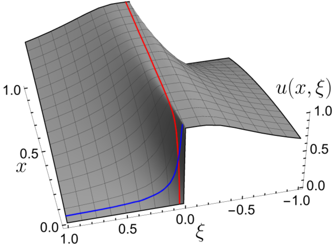
Fig. 2 clearly displays the boundary layer structure as $(x,\xi)\to(0^{+},0^{+})$.

The foremost two numerical methods used in the area, namely, the Spherical Harmonics Method and the Discrete Ordinates Method, see e.g. [6, Ch. 8] and [9, Ch. 3, 4], fail to properly resolve such boundary layer structures, as shown by recent attempts [10, 11, 12, 13, 14].

In view of the expression [15, p. 77] for the error term in Gauss–Legendre integration, the $\ell$–point quadrature error decreases like $32V/15\pi j(2\ell+1-j)^{j}$ provided the $j\leq 2\ell$ derivative of the integrated function is bounded by $V$. Introducing the change of variables $\xi^{\prime}=r^{p}$ in the integral in (1) we thus seek a bound $V$ on the $j$–th derivative of the resulting integrand. Using an integrated version of (1), similar to (4), combining two exponential terms and using the fact that for each non-negative integer $k$ the integral $\int_{0}^{\infty}t^{k}e^{-t}dt$ is finite, we find that

$$\begin{split}\left|\frac{\partial^{j}}{\partial r^{j}}\left[u(x,r^{p})r^{p-1}\right]\right|\leq Wr^{p-j-1}\;\text{as}\;(x,r)\to(0^{+},0^{+}),\end{split}$$

for some constant $W$; setting $V=Wr^{p-j-1}$ yields the desired bound, which, importantly, is uniform for all relevant values of $x$ and $r$ (as long as $p\geq j+1$).

In the case $\mathcal{R}(\xi)=0$ considered presently, splitting the integral on the right hand side of Eq. (1) at the boundary-layer point $\xi=0$ yields

$$\int_{0}^{1}u(x,\xi)d\xi\sim\sum_{i=1}^{M/2}w_{i}u(x,\xi_{i}),$$

(6)

where, letting $r_{i}$ and $w_{i}^{GL}$ denote the Gauss–Legendre quadrature abscissas and weights in the interval $[0,1]$, we have set $\xi_{i}=r_{i}^{p}$ and $w_{i}=p\times r_{i}^{p-1}\times w_{i}^{GL}/2$. The abscissas and weights corresponding to the negative values of $\xi$ are obtained by symmetry.

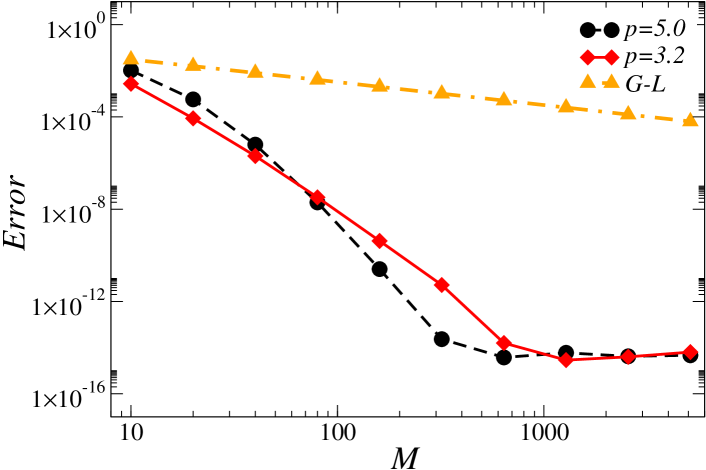
A suitable value $p=3.2$ was used, which provides excellent convergence (Fig. 3) for the integral in the $\xi$ variable while limiting the sharpness of the numerical boundary layer in the $x$ variable. The latter boundary layer is subsequently resolved by incorporating the logarithmic change of variables $v=\log(\frac{x}{1-x})$, thus giving rise to points $x$ extremely close to the boundary (without detriment to the integration process, in view of the $r$-derivative bounds mentioned above, which are uniform for all $x$), thus leading to high order precision in both the $\xi$ and $x$ variables.

The transport equation is solved in a computational spatial domain $[v_{\text{min}},v_{\text{max}}]$, with $[x^{\prime}_{\text{min}},x^{\prime}_{\text{max}}]=[\frac{e^{v_{\text{min}}}}{e^{v_{\text{min}}}+1},\frac{e^{v_{\text{max}}}}{e^{v_{\text{max}}}+1}]$, and with boundary conditions at $x^{\prime}_{\text{min}}$ and $x^{\prime}_{\text{max}}$ obtained by means of the asymptotic boundary layer solution (4). By using the new variables the time dependent transport problem

$$\begin{split}\frac{\partial}{\partial t}u(v,\xi,t)+&\xi(2+2\cosh(v))\frac{\partial}{\partial v}u(v,\xi,t)+\\ &\mu_{t}u(v,\xi,t)=\frac{\mu_{s}}{2}\int_{-1}^{1}u(v,\xi^{\prime},t)d\xi^{\prime}+q,\\ u(v,\xi,t_{\text{min}})&=0,\\ u(v_{\text{min}},\xi,t)&=u_{0}(x^{\prime}_{\text{min}},\xi,t)\;\forall\xi>0,\\ u(v_{\text{max}},\xi,t)&=u_{0}(x^{\prime}_{\text{max}},\xi,t)\;\forall\xi<0.\end{split}$$

(7)

results. The time propagation is performed implicitly by means of a third order backward differentiation formula (BDF). The collisional term is obtained by a polynomial extrapolation to avoid the inversion of large matrices at each time step. The discrete version of Eq. (7) reads

		$\displaystyle\left[\hat{\mathds{1}}+\beta\Delta t\xi_{j}(2+2\cosh(v))\hat{\mathds{D}}+\beta\Delta t\mu_{t}\hat{\mathds{1}}\right]u^{n+1}_{j}=$		(8)
		$\displaystyle\sum_{k=0}^{s-1}\alpha_{k}u_{j}^{n-k}+\beta\Delta t\frac{\mu_{s}}{2}\sum_{i=1}^{M}w_{i}\tilde{u}_{i}^{n+1}+\beta\Delta tq^{n+1},$

with $u^{n+1}_{j}=u(v,\xi_{j},t^{n+1})$, $t^{n+1}=n\Delta t$, where $\alpha_{k}$ and $\beta$ are the coefficients for the third order BDF formula, with $s=3$. The third order extrapolated quantity is given by $\tilde{u}_{j}^{n+1}=\sum_{\kappa=0}^{2}(-1)^{\kappa}{3\choose\kappa+1}u_{j}^{n-\kappa}$. The operator $\hat{\mathds{1}}$ is the identity operator while $\hat{\mathds{D}}$ is a spectral differentiation operator, which yields an implicit version of the Fourier Continuation–Discrete Ordinates Method (FC–DOM) developed by the authors [16].

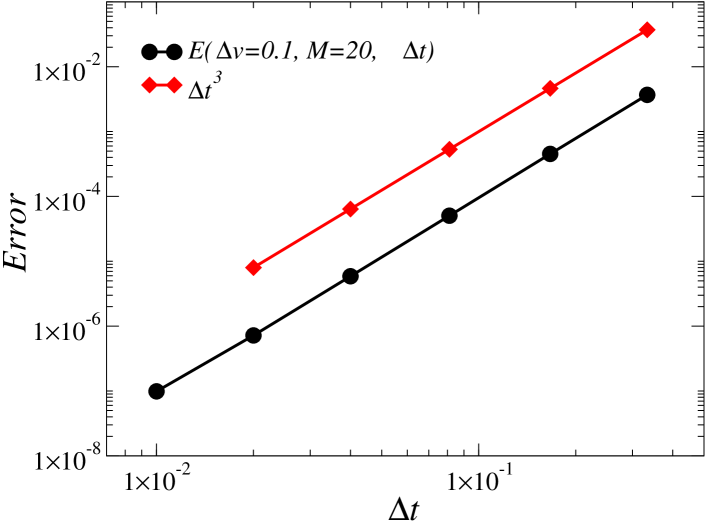
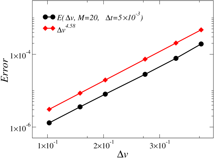
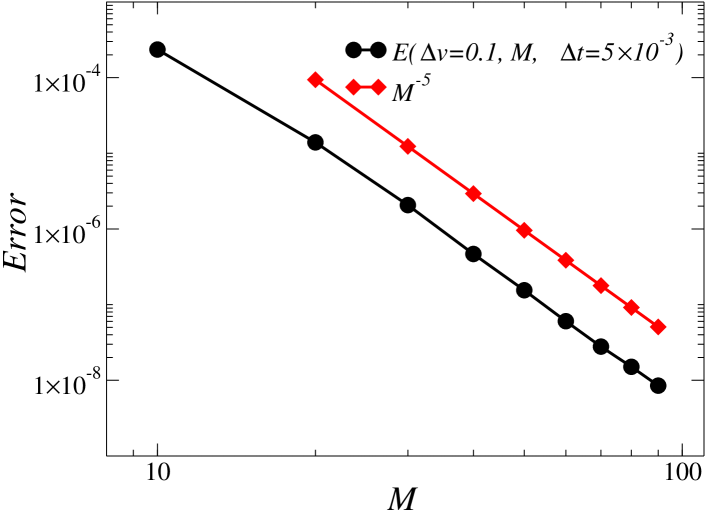
Fig. 4 demonstrates the excellent convergence properties of the algorithm, for $\mu_{s}=\mu_{a}=q=1$. Given that an analytic solution for problems including scattering is not known, the error was computed via comparison with the solution obtained on a finer grid. This high order of convergence clearly suggests that the changes of variables used in the $x$ and $\xi$ variables lead to adequate grid resolution of the boundary layers involved.

In what follows the numerical algorithm is utilized to explore and demonstrate the character of the boundary–layer structures considered in this paper. For definiteness, in the rest of this paper we restrict attention to time–independent solutions obtained by means of the time–dependent solver and letting the solution relax in time, as described in [16]. The resulting steady–state solutions are depicted in various forms in Figs. 5 through 7; similar boundary layer structures are of course present for all times in the time-dependent solutions.

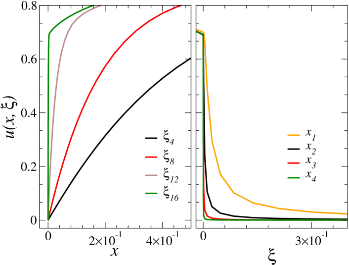
Fig. 5 presents boundary–layer structures in the $x$ and $\xi$ variables with $\mu_{s}=\mu_{a}=q=1$ (numerical parameter values $N=250$ and $M=40$ were used in these figures, with $-v_{\text{min}}=v_{\text{max}}=25$). As can be seen in Fig. 5, the smaller values of $\xi$ give boundary layers that shrinks over smaller spatial regions, as expected from our boundary layer analysis.

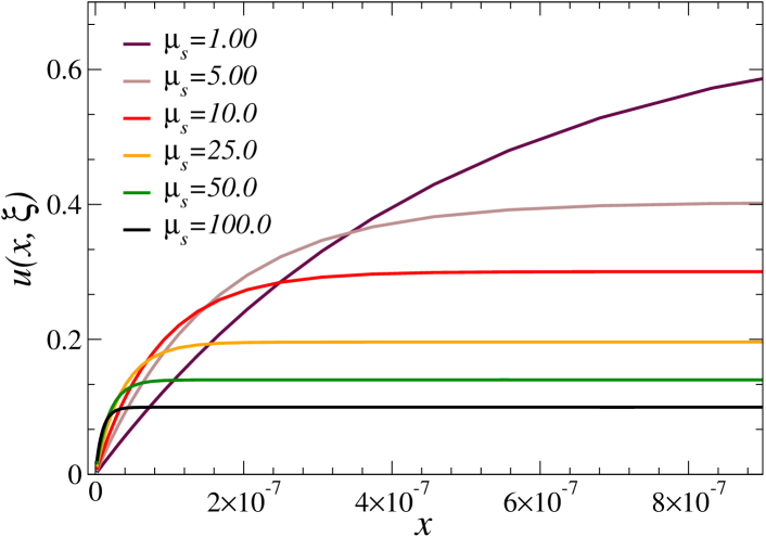
Fig. 6 demonstrates the persistence of the boundary layer even in presence of high scattering coefficient, with $\mu_{a}=q=1$ fixed. The case $\xi=\xi_{\text{min}}\simeq 10^{-6}$ is considered in the figure, with parameter values $N=200$, $M=20$ and $-v_{\text{min}}=v_{\text{max}}=20$. Clearly, even though diffusive problems (large $\mu_{s}$) tend to be more regular over the $\xi$ variable—owing to the strong averaging and smoothing induced by the large scattering coefficient—, the boundary layers that arise in the spatial variable with increasing $\mu_{s}$ tend to have larger slopes as $x\to 0^{+}$.

There have been many attempts to understand unphysical oscillations associated with the widely used Diamond finite Difference scheme (DD) for the transport equation [17, 18, 19]. The recent paper [11] avoids this problem by using only directions $\xi$ away from $\xi=0$. References [17, 18] attribute this type of oscillations to anisotropic boundary conditions, non diffusive boundary layers and/or high absorption; the present paper, which demonstrates existence of boundary layers even in the isotropic case and for all values of the scattering and absorption coefficients, presents a starkly contrasting interpretation. In particular, the present contribution explicitly demonstrates the existence of exponential boundary layers, triggered by the boundary condition and vanishing $\xi$ values, which are not considered in the previous discussions.

For example, reference [17] treats a diffusive transport problem (Problem 1 in that reference) which, under rescaling, can be reformulated as in Eq. (1) with $\mu_{s}=\mu_{t}=1000$, $q=0.1$ and $\mathcal{R}(\xi)=0$. This is an extremely diffusive problem with isotropic boundary conditions for which [17, pp. 317] states: “…since the leading order term in the asymptotic expansion of the analytic transport equation is itself isotropic, this term in these problems does not contain a boundary layer.” In contrast, Fig. 7 shows that boundary layers are present in this problem. The FC–DOM solution displayed in this figure was obtained by means of $M=40$ discrete directions and $N=400$ points in the spatial variable. In contrast, $N=10000$ were used in our DD-scheme solution presented in Fig. 7—which clearly displays the spurious oscillations produced by the DD scheme in this context.

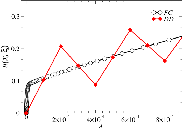
Physically, small values of $\xi$ along an incoming direction for points $x$ near the boundary (cf. Fig. 1) are associated to long geometrical particle paths which are not present for $x=0$, and which thus give rise to the sharp boundary-layer transition described in this paper. We emphasize that this boundary-layer structure, which was not previously reported in the literature, constitutes a physical effect which was mispredicted for nearly fifty years, and which, as demonstrated in Fig. 7 and throughout this paper, has a significant impact on the physics and the numerical simulation of transport phenomena.

OPB was supported by NSF through contract DMS-1714169 and by the NSSEFF Vannevar Bush Fellowship under contract number N00014-16-1-2808. ELG and DMM gratefully acknowledge the financial support from the following Argentine institutions: Consejo Nacional de Investigaciones Científicas y Técnicas (CONICET), PIP 11220130100607, Agencia Nacional de Promoción Científica y Tecnológica (ANPCyT) PICT–2017–2945, and Universidad de Buenos Aires UBACyT 20020170100727BA.

References

- [1] S. Chandrasekhar. Radiative Transfer. Dover, London, UK, first edition, 1960.
- [2] S. T. Thynell. Discrete-ordinates method in radiative heat transfer. International Journal of Engineering Science, 36(12-14):1651–1675, 1998.
- [3] E. G. Mishchenko and C. W. J. Beenakker. Radiative transfer theory for vacuum fluctuations. Physical Review Letters, 83(26):5475–5478, 1999.
- [4] O. N. Vassiliev, T. A. Wareing, J. McGhee, G. Failla, M. R. Salehpour, and F. Mourtada. Validation of a new grid-based Boltzmann equation solver for dose calculation in radiotherapy with photon beams. Physics in Medicine and Biology, 55(3):581–598, 2010.
- [5] J. Qin, J. J. Makela, F. Kamalabadi, and R. R. Meier. Radiative transfer modeling of the OI 135.6 nm emission in the nighttime ionosphere. Journal of Geophysical Research A: Space Physics, 120(11):10116–10135, 2015.
- [6] K. M. Case and P. F. Zweifel. Linear Transport Theory. Addison-Wesley, Reading, USA, first edition, 1967.
- [7] M. Born and E. Wolf. Principles of Optics. Cambridge University Press, London, UK, 60th anniversary edition, 2019.
- [8] C. M. Bender and S. A. Orszag. Advanced Mathematical Methods for Scientists and Engineers I. Springer–Verlag, New York, USA, first edition, 1999.
- [9] E. E. Lewis and W. F. Miller. Computational Methods of Neutron Transport. John Wiley & Sons, Hoboken, USA, first edition, 1984.
- [10] J. Rocheleau. An Analytical Nodal Discrete Ordinates Solution to the Transport Equation in Cartesian Geometry. Master thesis, 2020.
- [11] D. Wang and T. Byambaakhuu. High-Order Lax-Friedrichs WENO Fast Sweeping Methods for the Neutron Transport Equation. Nuclear Science and Engineering, 193(9):982–990, 2019.
- [12] R. Harel, S. Burov, and S. I. Heizler. Asymptotic Approximation in Radiative Transfer Problems. Journal of Computational and Theoretical Transport, 0(0):1–17, 2020.
- [13] F. Anli, F. Yaşa, S. Güngör, and H. Öztürk. approximation to neutron transport equation and application to critical slab problem. Journal of Quantitative Spectroscopy and Radiative Transfer, 101(1):129–134, 2006.
- [14] J. C. Chai, H. O. Lee, and S. V. Patankar. Ray effect and false scattering in the discrete ordinates method. Numerical Heat Transfer, Part B: Fundamentals, 24(4):373–389, 1993.
- [15] L. N. Trefethen. Is Gauss quadrature better than Clenshaw–Curtis? SIAM Review, 50(1):67–87, 2008.
- [16] E. L. Gaggioli, O. P. Bruno, and D. M. Mitnik. Light transport with the equation of radiative transfer: The Fourier Continuation – Discrete Ordinates (FC–DOM) Method. Journal of Quantitative Spectroscopy and Radiative Transfer, 236:106589, 2019.
- [17] E. W. Larsen, J. E. Morel, and W. F. Miller. Asymptotic solutions of numerical transport problems in optically thick, diffusive regimes. Journal of Computational Physics, 67(1):283–324, 1987.
- [18] B. G. Petrović and A. Haghighat. Analysis of inherent oscillations in multidimensional solutions of the neutron transport equation. Nuclear Science and Engineering, 124(1):31–62, 1996.
- [19] G. Bal. Fourier analysis of diamond discretization in particle transport. Calcolo, 38(3):141–172, 2001.