Few for Many: Tchebycheff Set Scalarization for Many-Objective Optimization

Xi Lin¹, Yilu Liu¹, Xiaoyuan Zhang¹, Fei Liu¹, Zhenkun Wang², Qingfu Zhang¹
¹City University of Hong Kong, ² Southern University of Science and Technology
[email protected], [email protected]

Abstract

Multi-objective optimization can be found in many real-world applications where some conflicting objectives can not be optimized by a single solution. Existing optimization methods often focus on finding a set of Pareto solutions with different optimal trade-offs among the objectives. However, the required number of solutions to well approximate the whole Pareto optimal set could be exponentially large with respect to the number of objectives, which makes these methods unsuitable for handling many optimization objectives. In this work, instead of finding a dense set of Pareto solutions, we propose a novel Tchebycheff set scalarization method to find a few representative solutions (e.g., 5) to cover a large number of objectives (e.g., $>100$ ) in a collaborative and complementary manner. In this way, each objective can be well addressed by at least one solution in the small solution set. In addition, we further develop a smooth Tchebycheff set scalarization approach for efficient optimization with good theoretical guarantees. Experimental studies on different problems with many optimization objectives demonstrate the effectiveness of our proposed method.

1 Introduction

In real-world applications, it is very often that many optimization objectives should be considered at the same time. Examples include manufacturing or engineering design with various specifications to achieve (Adriana et al., 2018; Wang et al., 2020), decision-making systems with different factors to consider (Roijers et al., 2014; Hayes et al., 2022), and molecular generation with multiple criteria to satisfy (Jain et al., 2023; Zhu et al., 2023). For a non-trivial problem, these optimization objectives conflict one another. Therefore, it is very difficult, if not impossible, for a single solution to accommodate all objectives at the same time (Miettinen, 1999; Ehrgott, 2005).

In the past several decades, much effort has been made to develop efficient algorithms for finding a set of Pareto solutions with diverse optimal trade-offs among different objectives. However, the Pareto set that contains all optimal trade-off solutions could be an manifold in the decision space, of which the dimensionality can be large for a problem with many objectives (Hillermeier, 2001). The number of required solutions to well approximate the whole Pareto set will increase exponentially with the number of objectives, which leads to prohibitively high computational overhead. In addition, a large solution set with high-dimensional objective vectors could easily become unmanageable for decision-makers. Indeed, a problem with more than $3$ objectives is already called the many-objective optimization problem (Fleming et al., 2005; Ishibuchi et al., 2008), and existing methods will struggle to deal with problems with a significantly larger number of optimization objectives (Sato & Ishibuchi, 2023).

In this work, instead of finding a dense set of Pareto solutions, we investigate a new approach for many-objective optimization, which aims to find a small set of solutions (e.g., $5$ ) to handle a large number of objectives (e.g., $>100$ ). In the optimal case, each objective should be well addressed by at least one solution in the small solution set as illustrated in Figure 1(d). This setting is important for different real-world applications with many objectives to optimize, such as finding complementary engineering designs to satisfy various criteria (Fleming et al., 2005), producing a few different versions of advertisements to serve a large group of diverse audiences (Matz et al., 2017; Eckles et al., 2018), and building a small set of models to handle many different data (Yi et al., 2014; Zhong et al., 2016) or tasks (Standley et al., 2020; Fifty et al., 2021). However, this demand has received little attention from the multi-objective optimization community. To properly handle this setting, this work makes the following contributions:

•

We propose a novel Tchebycheff set (TCH-Set) scalarization approach to find a few optimal solutions in a collaborative and complementary manner for many-objective optimization.
•

We further develop a smooth Tchebycheff set (STCH-Set) scalarization approach to tackle the non-smoothness of TCH-Set scalarization for efficient gradient-based optimization.
•

We provide theoretical analyses to show that our proposed approaches enjoy good theoretical properties for multi-objective optimization.
•

We conduct experiments on various multi-objective optimization problems with many objectives to demonstrate the efficiency of our proposed method. ¹¹1Our code to reproduce all experimental results will be released upon publication.

2 Preliminaries and Related Work

2.1 Multi-Objective Optimization

In this work, we consider the following multi-objective optimization problem:

\min_{\bm{x}\in\mathcal{X}}\ \bm{f}(\bm{x})=(f_{1}(\bm{x}),f_{2}(\bm{x}),\cdots,f_{m}(\bm{x})),

(1)

where $\bm{x}\in\mathcal{X}$ is a solution and $\bm{f}(\bm{x})=(f_{1}(\bm{x}),f_{2}(\bm{x}),\cdots,f_{m}(\bm{x}))\in\mathbb{R}^{m}$ are $m$ differentiable objective functions. For a non-trivial problem, there is no single solution $\bm{x}^{*}$ that can optimize all objective functions at the same time. Therefore, we have the following definitions of dominance, (weakly) Pareto optimality, and Pareto set/front for multi-objective optimization (Miettinen, 1999):

Definition 1 (Dominance and Strict Dominance).

Let $\bm{x}^{(a)},\bm{x}^{(b)}\in\mathcal{X}$ be two solutions for problem (1), $\bm{x}^{(a)}$ is said to dominate $\bm{x}^{(b)}$ , denoted as $\bm{f}(\bm{x}^{(a)})\prec\bm{f}(\bm{x}^{(b)})$ , if and only if $f_{i}(\bm{x}^{(a)})\leq f_{i}(\bm{x}^{(b)})\ \forall i\in\{1,...,m\}$ and $f_{j}(\bm{x}^{(a)})<f_{j}(\bm{x}^{(b)})\ \exists j\in\{1,...,m\}$ . In addition, $\bm{x}^{(a)}$ is said to strictly dominate $\bm{x}^{(b)}$ (i.e., $\bm{f}(\bm{x}^{(a)})\prec_{\text{strict}}\bm{f}(\bm{x}^{(b)})$ ), if and only if $f_{i}(\bm{x}^{(a)})<f_{i}(\bm{x}^{(b)})\ \forall i\in\{1,...,m\}$ .

Definition 2 ((Weakly) Pareto Optimality).

A solution $\bm{x}^{\ast}\in\mathcal{X}$ is Pareto optimal if there is no $\bm{x}\in\mathcal{X}$ such that $\bm{f}(\bm{x})\prec\bm{f}(\bm{x}^{\ast})$ . A solution $\bm{x}^{\prime}\in\mathcal{X}$ is weakly Pareto optimal if there is no $\bm{x}\in\mathcal{X}$ such that $\bm{f}(\bm{x})\prec_{\text{strict}}\bm{f}(\bm{x}^{\prime})$ .

Definition 3 (Pareto Set and Pareto Front).

The set of all Pareto optimal solutions $\bm{X}^{*}=\{\bm{x}\in\mathcal{X}|\bm{f}(\hat{}\bm{x})\nprec\bm{f}(\bm{x})\ \forall\hat{}\bm{x}\in\mathcal{X}\}$ is called the Pareto set. Its image in the objective space $\bm{f}(\bm{X}^{*})=\{\bm{f}(\bm{x})\in\mathbb{R}^{m}|\bm{x}\in\bm{X}^{*}\}$ is called the Pareto front.

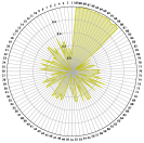
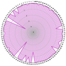
Under mild conditions, the Pareto set and front could be on an $(m-1)$ -dimensional manifold in the decision or objective space (Hillermeier, 2001), which contains infinite Pareto solutions. Many optimization methods have been proposed to find a finite set of solutions to approximate the Pareto set and front (Miettinen, 1999; Ehrgott, 2005; Zhou et al., 2011). If at least $k$ solutions are needed to handle each dimension of the Pareto front, the required number of solutions could be $O(k^{(m-1)})$ for a problem with $m$ optimization objectives. Two illustrative examples with a set of solutions to approximate the Pareto front for problems with $2$ and $3$ objectives are shown in Figure 1. However, the required number of solutions will increase exponentially with the objective number $m$ , leading to an extremely high computational overhead. It could also be very challenging for decision-makers to efficiently handle such a large set of solutions. Indeed, for a problem with many optimization objectives, a large portion of the solutions could become non-dominated and hence incomparable with each other (Purshouse & Fleming, 2007; Knowles & Corne, 2007).

In the past few decades, different heuristic and evolutionary algorithms have been proposed to tackle the many-objective black-box optimization problems (Zhang & Li, 2007; Bader & Zitzler, 2011; Deb & Jain, 2013). These algorithms typically aim to find a set of a few hundred solutions to handle problems with $4$ to a few dozen optimization objectives (Li et al., 2015; Sato & Ishibuchi, 2023). However, they still struggle to tackle problems with significantly many objectives (e.g., $>100$ ), and cannot efficiently solve large-scale differentiable optimization problems.

2.2 Gradient-based Multi-Objective Optimization

When all objective functions are differentiable with gradient $\{\nabla f_{i}(\bm{x})\}_{i=1}^{m}$ , we have the following definition for Pareto stationarity:

Definition 4 (Pareto Stationary Solution).

A solution $\bm{x}\in\mathcal{X}$ is Pareto stationary if there exists a set of weights $\bm{\alpha}\in\bm{\Delta}^{m-1}=\{\bm{\alpha}|\sum_{i=1}^{m}\alpha_{i}=1,\alpha_{i}\geq 0\ \forall i\}$ such that the convex combination of gradients $\sum_{i=1}^{m}\alpha_{i}\nabla f_{i}(\bm{x})=\bm{0}$ .

Multiple Gradient Descent Algorithm

One popular gradient-based approach is to find a valid gradient direction such that the values of all objective functions can be simultaneously improved (Fliege & Svaiter, 2000; Schäffler et al., 2002; Désidéri, 2012). The multiple gradient descent algorithm (MGDA) (Désidéri, 2012; Sener & Koltun, 2018) obtains a valid gradient $\bm{d}_{t}=\sum_{i=1}^{m}\alpha_{i}\nabla f_{i}(\bm{x})$ by solving the following quadratic programming problem at each iteration:

\displaystyle\min_{\alpha_{i}}||\sum\nolimits_{i=1}^{m}\alpha_{i}\nabla f_{i}(\bm{x}_{t})||_{2}^{2},~{}~{}~{}s.t.~{}\sum\nolimits_{i=1}^{m}\alpha_{i}=1,~{}~{}~{}\alpha_{i}\geq 0,\forall i=1,...,m,

(2)

and updates the current solution by a simple gradient descent $\bm{x}_{t+1}=\bm{x}_{t}-\eta_{t}\bm{d}_{t}$ . If $\bm{d}_{t}=\bm{0}$ , it means that there is no valid gradient direction that can improve all objectives at the same time, and therefore $\bm{x}_{t}$ is a Pareto stationary solution (Désidéri, 2012; Fliege et al., 2019). This idea has inspired many adaptive gradient methods for multi-task learning (Yu et al., 2020; Liu et al., 2021a; b; Momma et al., 2022; Liu et al., 2022; Navon et al., 2022; Senushkin et al., 2023; Lin et al., 2023; Liu et al., 2024). Different stochastic multiple gradient methods have also been proposed in recent years (Liu & Vicente, 2021; Zhou et al., 2022; Fernando et al., 2023; Chen et al., 2023; Xiao et al., 2023).

The location of solutions found by the original MGDA is not controllable, and several extensions have been proposed to find a set of diverse solutions with different trade-offs (Lin et al., 2019; Mahapatra & Rajan, 2020; Ma et al., 2020; Liu et al., 2021c). However, a large number of solutions is still required for a good approximation to the Pareto front. For solving problems with many objectives, MGDA and its extensions will suffer from a high computational overhead due to the high-dimensional quadratic programming problem (2) at each iteration. In addition, since a large portion of solutions is non-dominated with each other, it could be very hard to find a valid gradient direction to optimize all objectives at the same time.

Scalarization Method

Another popular class of methods for multi-objective optimization is the scalarization approach (Miettinen, 1999; Zhang & Li, 2007). The most straightforward method is linear scalarization (Geoffrion, 1967):

(Linear Scalarization)

\displaystyle\min_{\bm{x}\in\mathcal{X}}g^{(\text{LS})}(\bm{x}|\bm{\lambda})=\sum_{i=1}^{m}\lambda_{i}f_{i}(\bm{x}),

(3)

where $\bm{\lambda}=(\lambda_{1},\ldots,\lambda_{m})$ is a preference vector over $m$ objectives on the simplex $\bm{\Delta}^{m-1}=\{\bm{\lambda}|\sum_{i=1}^{m}\lambda_{i}=1,\lambda_{i}\geq 0\ \forall i\}$ . A set of diverse solutions can be obtained by solving the scalarization problem (3) with different preferences. Recently, different studies have shown that a well-tuned linear scalarization can outperform many adaptive gradient methods for multi-task learning Kurin et al. (2022); Xin et al. (2022); Lin et al. (2022); Royer et al. (2023). However, from the viewpoint of multi-objective optimization, linear scalarization cannot find any Pareto solution on the non-convex part of the Pareto front (Das & Dennis, 1997; Ehrgott, 2005; Hu et al., 2023).

Many other scalarization methods have been proposed in past decades. Among them, the Tchebycheff scalarization with good theoretical properties is a promising alternative (Bowman, 1976; Steuer & Choo, 1983):

(Tchebycheff Scalarization)

\displaystyle\min_{\bm{x}\in\mathcal{X}}g^{(\text{TCH})}(\bm{x}|\bm{\lambda})=\max_{1\leq i\leq m}\left\{\lambda_{i}(f_{i}(\bm{x})-z^{*}_{i})\right\},

(4)

where $\bm{\lambda}\in\bm{\Delta}^{m-1}$ is the preference and $\bm{z}^{*}\in\mathbb{R}^{m}$ is the ideal point (e.g., $z^{*}_{i}=\min f_{i}(\bm{x})-\epsilon$ with a small $\epsilon>0$ ). It is well-known that the Tchebycheff scalarization is able to find all weakly Pareto solutions for any Pareto front (Choo & Atkins, 1983). However, the $\max$ operator makes it become nonsmooth and hence suffers from a slow convergence rate by subgradient descent (Goffin, 1977) for differentiable multi-objective optimization. Recently, a smooth Tchebycheff scalarization approach (Lin et al., 2024) has been proposed to tackle the nonsmoothness issue:

(Smooth Tchebycheff Scalarization)

\displaystyle\min_{\bm{x}\in\mathcal{X}}g^{(\text{STCH})}_{\mu}(\bm{x}|\bm{\lambda})=\mu\log\left(\sum_{i=1}^{m}e^{\frac{\lambda_{i}(f_{i}(\bm{x})-z^{*}_{i})}{\mu}}\right),

(5)

where $\mu$ is the smooth parameter with a small positive value (e.g., $0.1$ ). According to (Lin et al., 2024), this smooth scalarization approach enjoys a fast convergence rate for the gradient-based method, while also having good theoretical properties for multi-objective optimization. A similar smooth optimization approach has also been proposed in He et al. (2024) for robust multi-task learning. Very recently, Qiu et al. (2024) prove and analyze the theoretical advantages of smooth Tchebycheff scalarization (5) over the classic Tchebycheff scalarization (4) for multi-objective reinforcement learning (MORL).

The scalarization methods do not have to solve a quadratic programming problem at each iteration and thus have lower pre-iteration complexity than MGDA. However, they still need to solve a large number of scalarization problems with different preferences to obtain a dense set of solutions to approximate the whole Pareto set.

3 Tchebycheff Set Scalarization for Many Objective Optimization

(a) Solution 1

(b) Solution 2

(d) Solution 4

(e) Solution 5

(f) All Solutions

Figure 2: Few Solutions to Address Many Optimization Objectives. (a)-(e):

5

different solutions to tackle different optimization objectives in a complementary manner. (f): They together successfully handle all

100

optimization objectives.

3.1 Small Solution Set for Many-Objective Optimization

Unlike previous methods, this work does not aim to find a huge set of solutions for approximating the whole Pareto set. Instead, we want to find a small set of solutions in a collaborative and complementary way such that each optimization objective can be well addressed by at least one solution. We have the following formulation of our targeted set optimization problem:

\min_{\bm{X}_{K}=\{\bm{x}^{(k)}\}_{k=1}^{K}}\bm{f}(\bm{x})=(\min_{\bm{x}\in\bm{X}_{K}}f_{1}(\bm{x}),\min_{\bm{x}\in\bm{X}_{K}}f_{2}(\bm{x}),\cdots,\min_{\bm{x}\in\bm{X}_{K}}f_{m}(\bm{x})),

(6)

where $\bm{X}_{K}=\{\bm{x}^{(k)}\}_{k=1}^{K}$ is a set of $K$ solutions to tackle all $m$ objectives $\{f_{i}(\bm{x})\}_{i=1}^{m}$ . With a large $K\geq m$ , we will have a degenerated problem:

\displaystyle\min_{\bm{X}_{K}}\bm{f}(\bm{x})=(\min_{\bm{x}^{(1)}\in\mathcal{X}}f_{1}(\bm{x}),\min_{\bm{x}^{(2)}\in\mathcal{X}}f_{2}(\bm{x}),\cdots,\min_{\bm{x}^{(m)}\in\mathcal{X}}f_{m}(\bm{x})),

(7)

where each objective function $f_{i}$ is independently solved by its corresponding solution $\bm{x}^{(i)}\in\mathcal{X}$ via single objective optimization and the rest $(K-m)$ solutions are redundant. If $K=1$ , the set optimization problem (6) will be reduced to the standard multi-objective optimization problem (1).

In this work, we are more interested in the case $1<K\ll m$ , which finds a small set of solutions (e.g., $K=5$ ) to tackle a large number of objectives (e.g., $m\geq 100$ ) as illustrated in Figure 2. In the ideal case, if the ground truth optimal objective group assignment is already known (e.g., which objectives should be optimized together by the same solution), it is straightforward to directly find an optimal solution for each group of objectives. However, for a general optimization problem, the ground truth objective group assignment is usually unknown in most cases, and finding the optimal assignment could be very difficult.

Very recently, a similar setting has been investigated in two concurrent works (Ding et al., 2024; Li et al., 2024).Ding et al. (2024) study the sum-of-minimum (SoM) optimization problem $\frac{1}{m}\sum_{i=1}^{m}\min\{f_{i}(\bm{x}^{(1)}),f_{i}(\bm{x}^{(2)}),\ldots,f_{i}(\bm{x}^{(K)})\}$ that can be found in many machine learning applications such as mixed linear regression (Yi et al., 2014; Zhong et al., 2016). They generalize the classic k-means++ (Arthur, 2007) and Lloyd’s algorithm (Lloyd, 1982) for clustering to tackle this problem, but do not take multi-objective optimization into consideration. Li et al. (2024) propose a novel Many-objective multi-solution Transport (MosT) framework to tackle many-objective optimization. With a bi-level optimization formulation, they adaptively construct a few weighted multi-objective optimization problems that are assigned to different representative regions on the Pareto front. By solving these weighted problems with MGDA, a diverse set of solutions can be obtained to well cover all objectives. In this work, we propose a straightforward and efficient set scalarization approach to explicitly optimize all objectives by a small set of solutions. A detailed experimental comparison with these methods can be found in Section 4.

3.2 Tchebycheff Set Scalarization

The set optimization formulation (6) is still a multi-objective optimization problem. In non-trivial cases, there is no single small solution set $\bm{X}_{K}$ with $K<m$ solutions that can optimize all $m$ objective functions $\{f_{i}(\bm{x})\}_{i=1}^{m}$ at the same time. To tackle this optimization problem, we propose the following Tchebycheff set (TCH-Set) scalarization approach:

	$\displaystyle\min_{\bm{X}_{K}=\{\bm{x}^{(k)}\}_{k=1}^{K}}g^{(\text{TCH-Set})}(\bm{X}_{K}\|\bm{\lambda})$	$\displaystyle=\max_{1\leq i\leq m}\left\{\lambda_{i}(\min_{\bm{x}\in\bm{X}_{K}}f_{i}(\bm{x})-z^{*}_{i})\right\}$
		$\displaystyle=\max_{1\leq i\leq m}\left\{\lambda_{i}(\min_{1\leq k\leq K}f_{i}(\bm{x}^{(k)})-z^{*}_{i})\right\},$		(8)

where $\bm{\lambda}=(\lambda_{1},\dots,\lambda_{m})$ and $\bm{z}^{*}=(z^{*}_{1},\dots,z^{*}_{m})$ are the preference and ideal point for each objective function. In this way, all objective values $\{f_{i}(\bm{x})\}_{i=1}^{m}$ among the whole solution set $\bm{X}_{K}=\{\bm{x}^{(k)}\}_{k=1}^{K}$ are scalarized into a single function $g^{(\text{TCH-Set})}(\bm{X}_{K}|\bm{\lambda})$ . In this work, a simple uniform vector $\bm{\lambda}=(\frac{1}{m},\ldots,\frac{1}{m})$ is used in all experiments without any specific preference among the objectives. A discussion on the effect of different preferences can be found in Appendix D.2.

By optimizing this TCH-Set scalarization function (8), we want to find an optimal small solution set $\bm{X}^{*}_{K}$ such that each objective can be well addressed by at least one solution $\bm{x}^{(k)}\in\bm{X}_{K}$ with a low worst objective value $\max_{1\leq i\leq m}\left\{\lambda_{i}(\min_{1\leq k\leq K}f_{i}(\bm{x}^{(k)})-z^{*}_{i})\right\}$ . When the solution set contains only one single solution (e.g., $K=1$ ), it will be reduced to the classic single-solution Tchebycheff scalarization (4). To avoid degenerated cases and focus on the key few-for-many setting, we make the following two assumptions in this work:

Assumption 1 (No Redundant Solution).

We assume that no solution in the optimal solution set $X^{*}_{K}=\mathtt{argmin}_{X_{k}}g^{(\text{TCH-Set})}(X_{K}|\lambda)$ will be redundant, which means

g^{(\text{TCH-Set})}(X^{*}_{K}|\lambda)<g^{(\text{TCH-Set})}(X^{*}_{K}\setminus\{x^{(k)}\}|\lambda)

(9)

holds for any $1\leq k\leq K\leq m$ with $\lambda>\bm{0}$ .

Assumption 2 (All Positive Preference).

In the few-for-many setting, we assume that the preferences should be positive for all objectives such that $\{\sum_{i=1}^{m}\lambda_{i}=1,\lambda_{i}>0\ \forall i\}$ .

These assumptions are reasonable in practice, especially for the few-for-many setting (e.g., $K\ll m$ ) considered in this work. For a general problem, it is extremely rare that a small number of solutions (e.g., $4$ ) can exactly solve a large number of objectives (e.g., $m=1,000$ ). From the viewpoint of clustering (Ding et al., 2024), it is analogous to the case that all the $1,000$ data points under consideration are exactly located in $4$ different locations. If we do meet this extreme case with $p$ redundant solutions, we can simply reduce the number of solutions to make it a $(K-p)$ -solutions-for- $m$ -objectives problem. Similarly, if some of the preferences (e.g., $q$ ) are $0$ , we can also simply reduce the original $m$ -objective problem into a $(m-q)$ -objective problem that satisfies the positive preference assumption.

From the viewpoint of multi-objective optimization, we have the following guarantee for the optimal solution set of Tchebycheff set scalarization:

Theorem 1 (Existence of Pareto Optimal Solution for Tchebycheff Set Scalarization).

There exists an optimal solution set $\bar{}\bm{X}^{*}_{K}$ for the Tchebycheff set scalarization optimization problem (8) such that all solutions in $\bar{}\bm{X}^{*}_{K}$ are Pareto optimal of the original multi-objective optimization problem (1). In addition, if the optimal set $\bm{X}^{*}_{K}$ is unique, all solutions in $\bm{X}^{*}_{K}$ are Pareto optimal.

Proof Sketch.

This theorem can be proved by construction and contradiction based on Definition 2 for (weakly) Pareto optimality and the form of Tchebycheff set Scalarization (8). A detailed proof is provided in Appendix A.1. ∎

It should be emphasized that, without the strong unique optimal solution set assumption, we only have a weak existence guarantee for the Pareto optimality. For an optimal solution set for the Tchebycheff set scalarization (8), it is possible that many of the solutions are not even weakly Pareto optimal for the original multi-objective optimization problem (1). This finding could be a bit surprising for multi-objective optimization, and we provide a detailed discussion in Appendix A.5. In addition to the Pareto optimality guarantee, the non-smoothness of TCH-Set scalarization might also hinder its practical usage for efficient optimization. To address these crucial issues, we further develop a smooth Tchebycheff set scalarization with good optimization property and promising Pareto optimality guarantee in the next subsection.

3.3 Smooth Tchebycheff Set Scalarization

The Tchebycheff set scalarization formulation (8) involves a $\max$ and a $\min$ operator, which leads to its non-smoothness even when all objective functions $\{f_{i}(\bm{x})\}_{i=1}^{m}$ are smooth. In other words, the Tchebycheff set scalarization $g^{(\text{TCH-Set})}(\bm{X}_{K}|\bm{\lambda})$ is not differentiable and will suffer from a slow convergence rate by subgradient descent. To address this issue, we leverage the smooth optimization approach (Nesterov, 2005; Beck & Teboulle, 2012; Chen, 2012) to propose a smooth Tchebycheff set scalarization for multi-objective optimization.

According to Beck & Teboulle (2012), for the maximization function among all objectives $\max_{1\leq i\leq m}\{f_{1}(\bm{x}),f_{2}(\bm{x}),\ldots,f_{m}(\bm{x})\}$ , we have the smooth maximization function:

\operatorname*{smax}_{1\leq i\leq m}\{f_{1}(\bm{x}),f_{2}(\bm{x}),\ldots,f_{m}(\bm{x})\}=\mu\log\left(\sum_{i=1}^{m}e^{\frac{f_{i}(\bm{x})}{\mu}}\right),

(10)

where $\mu$ is a smooth parameter. Similarly, for the minimization among different solutions for the $i$ -th objective $\min_{1\leq k\leq K}\{f_{i}(\bm{x}^{(1)}),f_{i}(\bm{x}^{(2)}),\ldots,f_{i}(\bm{x}^{(K)})\}$ , we have the smooth minimization function:

\operatorname*{smin}_{1\leq k\leq K}\{f_{i}(\bm{x}^{(1)}),f_{i}(\bm{x}^{(2)}),\ldots,f_{i}(\bm{x}^{(K)})\}=-\mu_{i}\log\left(\sum_{k=1}^{K}e^{-\frac{f_{i}(\bm{x}^{(k)})}{\mu_{i}}}\right),

(11)

where $\mu_{i}$ is a smooth parameter.

By leveraging the above smooth maximization and minimization functions, we propose the smooth Tchebycheff set scalarization (STCH-Set) scalarization for multi-objective optimization:

$\displaystyle\min_{\bm{X}_{K}=\{\bm{x}^{(k)}\}_{k=1}^{K}}g_{\mu,\{\mu_{i}\}_{i=1}^{m}}^{(\text{STCH-Set})}(\bm{X}_{K}\|\bm{\lambda})$	$\displaystyle=\operatorname{smax}_{1\leq i\leq m}\left\{\lambda_{i}\operatorname{smin}\limits_{1\leq k\leq K}f_{i}(\bm{x}^{(k)})-z^{*}_{i}\right\}$
	$\displaystyle=\mu\log\left(\sum_{i=1}^{m}e^{\frac{\lambda_{i}\left(\operatorname{smin}\limits_{1\leq k\leq K}f_{i}(\bm{x}^{(k)})-z^{}_{i}\right)}{\mu}}\right)$
	$\displaystyle=\mu\log\left(\sum_{i=1}^{m}e^{\frac{\lambda_{i}\left(-\mu_{i}\log\left(\sum_{k=1}^{K}e^{-{f_{i}(\bm{x}^{(k)})}/{\mu_{i}}}\right)-z^{*}_{i}\right)}{\mu}}\right).$	(12)

If the same smooth parameter $\mu_{1}=\ldots=\mu_{m}=\mu$ are used for all smooth terms, we have the following simplified formulation:

\min_{\bm{X}_{K}=\{\bm{x}^{(k)}\}_{k=1}^{K}}g_{\mu}^{(\text{STCH-Set})}(\bm{X}_{K}|\bm{\lambda})=\mu\log\left(\sum_{i=1}^{m}e^{\lambda_{i}\left(-\log\left(\sum_{k=1}^{K}e^{-{f_{i}(\bm{x}^{(k)})}/{\mu}}\right)-z^{*}_{i}\right)}\right).

(13)

When $K=1$ , it will reduce to the single-solution smooth Tchebycheff scalarization (5). Similarly to the non-smooth TCH-Set counterpart, the STCH-Set scalarization also has good theoretical properties for multi-objective optimization:

Theorem 2 (Pareto Optimality for Smooth Tchebycheff Set Scalarization).

All solutions in the optimal solution set $\bm{X}^{*}_{K}$ for the smooth Tchebycheff set scalarization problem (12) are weakly Pareto optimal of the original multi-objective optimization problem (1). In addition, the solutions are Pareto optimal if either

1.

the optimal solution set $\bm{X}^{*}_{K}$ is unique, or
2.

all preference coefficients are positive ( $\lambda_{i}>0\ \forall i$ ).

Proof Sketch.

This theorem can be proved by contradiction based on Definition 2 for (weakly) Pareto optimality and the form of smooth Tchebycheff set scalarization (12). We provide a detailed proof in Appendix A.2. ∎

Theorem 3 (Uniform Smooth Approximation).

The smooth Tchebycheff set (STCH-Set) scalarization $g_{\mu,\{\mu_{i}\}_{i=1}^{m}}^{(\text{STCH-Set})}(\bm{X}_{K}|\bm{\lambda})$ is a uniform smooth approximation of the Tchebycheff set (TCH-Set) scalarization $g^{(\text{TCH-Set})}(\bm{X}_{K}|\bm{\lambda})$ , and we have:

\lim_{\mu\downarrow 0,\mu_{i}\downarrow 0\ \forall i}g_{\mu,\{\mu_{i}\}_{i=1}^{m}}^{(\text{STCH-Set})}(\bm{X}_{K}|\bm{\lambda})=g^{(\text{TCH-Set})}(\bm{X}_{K}|\bm{\lambda})

(14)

for any valid set $\bm{X}_{k}\subset\mathcal{X}$ .

Proof Sketch.

This theorem can be proved by deriving the upper and lower bounds of the TCH-Set scalarization $g^{(\text{TCH-Set})}(\bm{X}_{K}|\bm{\lambda})$ with respect to the smooth $\operatorname*{smax}$ and $\operatorname*{smin}$ operators in the STCH-Set scalarization $g_{\mu,\{\mu_{i}\}_{i=1}^{m}}^{(\text{STCH-Set})}(\bm{X}_{K}|\bm{\lambda})$ . A detailed proof is provided in Appendix A.3. ∎

According to these theorems, for any smooth parameters $\mu$ and $\{\mu\}_{i=1}^{m}$ , all solutions in the optimal set $\bm{X}^{*}_{K}$ for STCH-Set scalarization (12) are also (weakly) Pareto optimal. In addition, with small smooth parameters $\mu\downarrow 0,\mu_{i}\downarrow 0\ \forall i$ , the value of $g_{\mu,\{\mu_{i}\}_{i=1}^{m}}^{(\text{STCH-Set})}(\bm{X}_{K}|\bm{\lambda})$ will be close to its non-smooth counterpart $g^{(\text{TCH-Set})}(\bm{X}_{K}|\bm{\lambda})$ for all valid solution sets $\bm{X}_{K}$ , which is also the case for the optimal set $\bm{X}^{*}_{K}=\operatorname*{arg\,min}_{\bm{X}_{K}}g^{(\text{TCH-Set})}(\bm{X}_{K}|\bm{\lambda})$ . Therefore, it is reasonable to find an approximate optimal solution set for the original $g^{(\text{TCH-Set})}(\bm{X}_{K}|\bm{\lambda})$ by optimizing its smooth counterpart $g_{\mu,\{\mu_{i}\}_{i=1}^{m}}^{(\text{STCH-Set})}(\bm{X}_{K}|\bm{\lambda})$ with small smooth parameters $\mu$ and $\{\mu_{i}\}_{i=1}^{m}$ .

Algorithm 1 STCH-Set Scalarization for Multi-Objective Optimization

1: Input: Preference

\bm{\lambda}

, Step Size

\{\eta_{t}\}_{t=0}^{T}

, Initial

\bm{X}^{0}_{K}

2: for

t=1

T

\bm{X}^{t}_{K}=\bm{X}^{t-1}_{K}-\eta_{t}\nabla g^{(\text{STCH-Set})}(\bm{X}^{t-1}_{K}|\bm{\lambda})

4: end for

5: Output: Final Solution

\bm{X}^{T}_{K}

The STCH-Set scalarization function $g_{\mu,\{\mu_{i}\}_{i=1}^{m}}^{(\text{STCH-Set})}(\bm{X}_{K}|\bm{\lambda})$ can be efficiently optimized by any gradient-based optimization method. A simple gradient descent algorithm for STCH-Set is shown in Algorithm 1. However, when the objective functions $\{f_{i}(\bm{x})\}_{i=1}^{m}$ are highly non-convex, it could be very hard to find the global optimal set $\bm{X}^{*}_{K}$ for $g_{\mu,\{\mu_{i}\}_{i=1}^{m}}^{(\text{STCH-Set})}(\bm{X}_{K}|\bm{\lambda})$ . In this case, we have the Pareto stationarity guarantee for the gradient-based method:

Theorem 4 (Convergence to Pareto Stationary Solution).

If there exists a solution set $\hat{}\bm{X}_{K}$ such that $\nabla_{\hat{}\bm{x}^{(k)}}g_{\mu,\{\mu_{i}\}_{i=1}^{m}}^{(\text{STCH-Set})}(\hat{}\bm{X}_{K}|\bm{\lambda})=\bm{0}$ for all $\hat{}\bm{x}^{(k)}\in\hat{}\bm{X}_{K}$ , then all solutions in $\hat{}\bm{X}_{K}$ are Pareto stationary solutions of the original multi-objective optimization problem (1).

Proof Sketch.

We can prove this theorem by analyzing the form of gradient for STCH-Set scalarization $\nabla_{\hat{}\bm{x}^{(k)}}g_{\mu,\{\mu_{i}\}_{i=1}^{m}}^{(\text{STCH-Set})}(\hat{}\bm{X}_{K}|\bm{\lambda})=\bm{0}$ for each solution $\bm{x}^{(k)}$ with the condition for Pareto stationarity in Definition 4. A detailed proof is provided in Appendix A.4. ∎

When $K$ reduces to $1$ , all these theorems exactly match their counterpart theorems for single-solution smooth Tchebycheff scalarization (Lin et al., 2024).

Table 1: The results on convex optimization problems with

K=\{3,4,5,6,8,10\}

solutions. Mean worst and average objective values over

50

runs are reported. Best results are highlighted in bold, and the full table can be found in Appendix C.1.

number of objectives $m=128$
		LS	TCH	STCH	MosT	SoM	TCH-Set	STCH-Set
	worst	4.64e+00(+)	4.44e+00(+)	4.41e+00(+)	2.12e+00(+)	1.86e+00(+)	1.02e+00(+)	6.08e-01
K = 3	average	8.61e-01(+)	8.03e-01(+)	7.80e-01(+)	3.45e-01(+)	2.02e-01(-)	3.46e-01(+)	2.12e-01
	worst	4.23e+00(+)	3.83e+00(+)	3.68e+00(+)	1.48e+00(+)	1.12e+00(+)	6.74e-01(+)	3.13e-01
K = 4	average	7.45e-01(+)	6.54e-01(+)	6.41e-01(+)	1.85e-01(+)	1.12e-01(+)	2.27e-01(+)	9.44e-02
	worst	4.17e+00(+)	3.56e+00(+)	3.51e+00(+)	1.02e+00(+)	9.20e-01(+)	4.94e-01(+)	1.91e-01
K = 5	average	7.08e-01(+)	5.75e-01(+)	5.05e-01(+)	9.81e-02(+)	7.95e-02(+)	1.60e-01(+)	5.12e-02
	worst	3.81e+00(+)	3.41e+00(+)	3.20e+00(+)	9.56e-01(+)	7.03e-01(+)	3.72e-01(+)	1.36e-01
K = 6	average	6.72e-01(+)	5.31e-01(+)	5.15e-01(+)	8.34e-02(+)	5.34e-02(+)	1.19e-01(+)	3.15e-02
	worst	3.69e+00(+)	2.94e+00(+)	2.61e+00(+)	8.32e-01(+)	5.20e-01(+)	2.84e-01(+)	1.02e-01
K = 8	average	6.16e-01(+)	4.57e-01(+)	4.22e-01(+)	6.91e-02(+)	3.40e-02(+)	8.53e-02(+)	1.78e-02
	worst	3.68e+00(+)	2.69e+00(+)	2.40e+00(+)	6.27e-01(+)	4.07e-01(+)	1.95e-01(+)	7.99e-02
K = 10	average	5.69e-01(+)	4.07e-01(+)	3.20e-01(+)	4.59e-02(+)	2.43e-02(+)	5.92e-02(+)	1.34e-02
Wilcoxon Rank-Sum Test Summary
	worst	6/0/0	6/0/0	6/0/0	6/0/0	6/0/0	6/0/0	-
+/=/-	average	6/0/0	6/0/0	6/0/0	6/0/0	5/0/1	6/0/0	-

4 Experiments

Baseline Methods

In this section, we compare our proposed TCH-Set and STCH-Set scalarization with three simple scalarization methods: (1) linear scalarization (LS) with randomly sampled preferences, (2) Tchebycheff scalarization (TCH) with randomly sampled preferences, (3) smooth Tchebycheff scalarization (STCH) with randomly sampled preferences (Lin et al., 2024), as well as two recently proposed methods for finding a small set of solutions: (4) the many-objective multi-solution transport (MosT) method (Li et al., 2024), and (5) the efficient sum-of-minimum (SoM) optimization method (Ding et al., 2024).

Experimental Setting

This work aims to find a small set $\bm{X}_{K}$ with $K$ solutions to address all $m$ objectives in each problem. For each objective $f_{i}(\bm{x})$ , we care about the best objective value $\min_{\bm{x}\in\bm{X}_{K}}f_{i}(\bm{x})$ achieved by the solutions in $\bm{X}_{K}$ . Both the worst obtained value among all objectives $\max_{1\leq i\leq m}\min_{\bm{x}\in\bm{X}_{K}}f_{i}(\bm{x})$ and the average objective value $\frac{1}{m}\sum_{i=1}^{m}\min_{\bm{x}\in\bm{X}_{K}}f_{i}(\bm{x})$ are reported for comparison. Detailed experimental settings for each problem can be found in Appendix B. Due to the page limit, more experimental results and analysis can be found in Appendix C.

4.1 Experimental Results and Analysis

Convex Many-Objective Optimization

We first test our proposed methods for solving convex multi-objective optimization with $m=128$ or $m=1,024$ objective functions with different numbers of solutions (from $3$ to $20$ ). We independently run each comparison $50$ times. In each run, we randomly generate $m$ independent convex quadratic functions as the optimization objectives for all methods. The mean worst and average objective values for each method over $50$ runs on the $m=128$ case are reported in Table 1 and the full table can be found in Appendix C.1. We also conduct the Wilcoxon rank-sum test between STCH-Set and other methods for all comparisons at the $0.05$ significant level. The $(+/=/-)$ symbol means the result obtained by STCH-Set is significantly better, equal to, or worse than the results of the compared method.

According to the results, the traditional methods (e.g., LS/TCH/STCH) fail to properly tackle the few solutions for many objectives setting considered in this work. MosT achieves much better performance than the traditional methods by actively finding a set of diverse solutions to cover all objectives, but it cannot tackle the problems with $1024$ objectives in a reasonable time. In addition, MosT is outperformed by SoM and our proposed STCH-Set, which directly optimizes the performance for each objective. Our proposed STCH-Set performs the best in achieving the low worst objective values for all comparisons. In addition, although not explicitly designed, STCH-Set also achieves a very promising mean average performance for most comparisons since all objectives are well addressed. The importance of smoothness for set optimization is fully confirmed by the observation that STCH-Set significantly outperforms TCH-Set on all comparisons. More discussion on why STCH-Set can outperform SoM on the average performance can be found in Appendix D.4.

Table 2: The results on mixed linear regression with noisy level

\sigma=0.1

. Full table in Appendix C.2.

		LS	TCH	STCH	SoM	TCH-Set	STCH-Set
K = 5	worst	3.84e+01(+)	2.45e+01(+)	2.43e+01(+)	2.50e+00(+)	4.19e+00(+)	2.10e+00
	average	2.70e+00(+)	1.46e+00(+)	1.44e+00(+)	1.88e-01(-)	6.53e-01(+)	4.72e-01
	worst	2.21e+01(+)	2.49e+01(+)	3.92e+01(+)	3.46e+00(+)	2.04e+00(+)	5.00e-01
K = 10	average	1.09e+00(+)	1.19e+00(+)	3.01e+00(+)	2.33e-01(+)	3.83e-01(+)	2.00e-01
	worst	4.20e+01(+)	2.11e+01(+)	2.21e+01(+)	2.57e+00(+)	1.64e+00(+)	2.70e-01
K = 15	average	3.07e+00(+)	1.02e+00(+)	1.02e+00(+)	1.97e-01(+)	3.22e-01(+)	1.66e-01
	worst	4.20e+01(+)	2.14e+01(+)	2.04e+01(+)	1.44e+00(+)	1.79e+00(+)	2.27e-01
K = 20	average	3.09e+00(+)	8.35e-01(+)	8.87e-01(+)	1.84e-01(+)	3.29e-01(+)	1.66e-01

Noisy Mixed Linear Regression

We then test different methods’ performance on the noisy mixed linear regression problem as in (Ding et al., 2024). For each comparison, $1,000$ data points are randomly generated from $K$ ground truth linear models with noise. Then, with different optimization methods, we train $K$ linear regression models to tackle all $1,000$ data points where the objectives are the squared error for each point. Each comparison are run $50$ times, and the detailed experiment setting is in Appendix B.

We conduct comparison with different numbers of $K=\{5,10,15,20\}$ and noise levels $\sigma=\{0.1,0.5,1.0\}$ . The results with $\sigma=0.1$ are shown in Table 2, and the full results can be found in Appendix C.2. According to the results, our proposed STCH-Set can always achieve the lowest worst objective value, and achieves the best average objective value in most comparisons.

Table 3: Results on mixed nonlinear regression with noisy level

\sigma=0.1

. Full table in Appendix C.3.

		LS	TCH	STCH	SoM	TCH-Set	STCH-Set
K = 5	worst	2.34e+02 (+)	1.68e+02(+)	1.57e+02(+)	1.68e+01(+)	1.94e+01(+)	7.43e+00
	average	9.19e+00(+)	8.50e+00(+)	7.90e+00(+)	8.54e-01(-)	3.48e+00(+)	1.89e+00
	worst	3.23e+02(+)	1.72e+02(+)	1.57e+02(+)	4.42e+00(+)	6.07e+00(+)	6.28e-01
K = 10	average	8.70e+00 (+)	6.65e+00(+)	5.85e+00(+)	1.22e-01(+)	1.03e+00(+)	5.99e-02
	worst	3.65e+02(+)	2.10e+02(+)	1.62e+02(+)	1.10e+00(+)	1.57e+00(+)	2.05e-01
K = 15	average	8.33e+00(+)	5.66e+00(+)	4.89e+00(+)	1.47e-01(+)	3.27e-01(+)	1.27e-02
	worst	3.36e+02(+)	2.04e+02(+)	1.81e+02(+)	5.59e+00(+)	4.37e+00(+)	6.22e-01
K = 20	average	8.81e+00(+)	6.92e+00(+)	6.23e+00(+)	1.24e-01(+)	9.09e-01(+)	6.27e-02

Noisy Mixed Nonlinear Regression

Following (Ding et al., 2024), we also compare different methods on the noisy mixed nonlinear regression. The problem setting (details in Appendix B) is similar to the mixed linear regression, but we now build nonlinear neural networks as the models. According to the results in Table 3 and Appendix C.3, STCH-Set can still obtain the best overall performance for most comparisons. We visualize different methods’ performance on $100$ sampled data in Figure 3, and it is clear that STCH-Set can well address all objectives with the best overall performance.

Table 4: Results on training

K

models to handle

9

different tasks on the Celeb-A datasets. Here we report the worst and average pre-task classification among the

9

task.

		RG*	HOA*	TAG*	DMTG*	SoM	TCH-Set	STCH-Set
K = 2	worst	-	-	-	12.18	12.08	11.99	11.89
	average	6.09	5.96	5.93	5.89	5.80	5.86	5.81
	worst	-	-	-	12.26	12.15	12.06	11.98
K = 3	average	6.06	6.00	6.04	5.96	5.89	5.98	5.89
	worst	-	-	-	12.37	12.32	12.18	12.05
K = 4	average	6.06	6.02	6.01	5.96	5.90	5.99	5.92

Deep Multi-Task Grouping

We evaluate STCH-Set’s performance on finding a few deep multi-task learning models ( $K=\{2,3,4\}$ ) to separately handle $9$ different tasks on the Celeb-A datasets (Liu et al., 2015) following the setting in Gao et al. (2024) (details in Appendix B). The results of four typical multi-task grouping methods (Random Grouping, HOA (Standley et al., 2020), TAG (Fifty et al., 2021) and DMTG (Gao et al., 2024)) are directly from Gao et al. (2024). According to the results in Table 4, STCH-Set can successfully optimize the worst task performance and also achieve good average performance (slightly worse than SoM in two cases) with different number of models. The performance of SoM, TCH-Set, and STCH-Set might be further improved with fine-tuned hyperparameters rather than those used for DMTG.

5 Conclusion, Limitation and Future Work

Conclusion

In this work, we have proposed a novel Tchebycheff set (TCH-Set) scalarization and a smooth Tchebycheff set (STCH-Set) scalarization to find a small set of solutions for many-objective optimization. When properly optimized, each objective in the original problem should be well addressed by at least one solution in the found solution set. Both theoretical analysis and experimental studies have been conducted to demonstrate the promising properties and efficiency of TCH-Set/STCH-Set. Our proposed methods could provide a promising alternative to the current methods for tackling many-objective optimization.

Limitation and Future Work

This work proposes a general optimization method for multi-objective optimization which are not tied to particular applications. We do not see any specific potential societal impact of the proposed methods. This work only focuses on the deterministic optimization setting that all objectives are always available. One potential future research direction is to investigate how to deal with only partially observable objective values in practice.

References

Ackerman et al. (2012) Margareta Ackerman, Shai Ben-David, Simina Brânzei, and David Loker. Weighted clustering. In AAAI Conference on Artificial Intelligence (AAAI), 2012.
Adriana et al. (2018) Schulz Adriana, Wang Harrison, Crinspun Eitan, Solomon Justin, and Matusik Wojciech. Interactive exploration of design trade-offs. Acm Transactions on Graphics, 37(4):1–14, 2018.
Arthur (2007) David Arthur. K-means++: The advantages of careful seeding. In Proc. Eighteenth Annual ACM-SIAM Symposium on Discrete Algorithms, pp. 1027–1035, 2007.
Bader & Zitzler (2011) Johannes Bader and Eckart Zitzler. Hype: An algorithm for fast hypervolume-based many-objective optimization. Evolutionary computation, 19(1):45–76, 2011.
Beck & Teboulle (2012) Amir Beck and Marc Teboulle. Smoothing and first order methods: A unified framework. SIAM Journal on Optimization, 22(2):557–580, 2012.
Bertsekas et al. (2003) Dimitri Bertsekas, Angelia Nedic, and Asuman Ozdaglar. Convex analysis and optimization, volume 1. Athena Scientific, 2003.
Bowman (1976) V Joseph Bowman. On the relationship of the tchebycheff norm and the efficient frontier of multiple-criteria objectives. In Multiple criteria decision making, pp. 76–86. Springer, 1976.
Boyd & Vandenberghe (2004) Stephen Boyd and Lieven Vandenberghe. Convex optimization. Cambridge university press, 2004.
Chen et al. (2023) Lisha Chen, Heshan Fernando, Yiming Ying, and Tianyi Chen. Three-way trade-off in multi-objective learning: Optimization, generalization and conflict-avoidance. In Advances in Neural Information Processing Systems (NeurIPS), 2023.
Chen (2012) Xiaojun Chen. Smoothing methods for nonsmooth, nonconvex minimization. Mathematical programming, 134:71–99, 2012.
Choo & Atkins (1983) Eng Ung Choo and DR Atkins. Proper efficiency in nonconvex multicriteria programming. Mathematics of Operations Research, 8(3):467–470, 1983.
Das & Dennis (1997) Indraneel Das and J.E. Dennis. A closer look at drawbacks of minimizing weighted sums of objectives for pareto set generation in multicriteria optimization problems. Structural Optimization, 14(1):63–69, 1997.
Deb & Jain (2013) Kalyanmoy Deb and Himanshu Jain. An evolutionary many-objective optimization algorithm using reference-point-based nondominated sorting approach, part i: solving problems with box constraints. IEEE transactions on evolutionary computation, 18(4):577–601, 2013.
Désidéri (2012) Jean-Antoine Désidéri. Mutiple-gradient descent algorithm for multiobjective optimization. In European Congress on Computational Methods in Applied Sciences and Engineering (ECCOMAS 2012), 2012.
Ding et al. (2024) Lisang Ding, Ziang Chen, Xinshang Wang, and Wotao Yin. Efficient algorithms for sum-of-minimum optimization. In International Conference on Machine Learning (ICML), 2024.
Dunlavy & O’Leary (2005) Daniel M. Dunlavy and Dianne P. O’Leary. Homotopy optimization methods for global optimization. In Technical Report, 2005.
Eckles et al. (2018) Dean Eckles, Brett R Gordon, and Garrett A Johnson. Field studies of psychologically targeted ads face threats to internal validity. Proceedings of the National Academy of Sciences, 115(23):E5254–E5255, 2018.
Ehrgott (2005) Matthias Ehrgott. Multicriteria optimization, volume 491. Springer Science & Business Media, 2005.
Fernando et al. (2023) Heshan Devaka Fernando, Han Shen, Miao Liu, Subhajit Chaudhury, Keerthiram Murugesan, and Tianyi Chen. Mitigating gradient bias in multi-objective learning: A provably convergent approach. In International Conference on Learning Representations (ICLR), 2023.
Fifty et al. (2021) Christopher Fifty, Ehsan Amid, Zhe Zhao, Tianhe Yu, Rohan Anil, and Chelsea Finn. Efficiently identifying task groupings for multi-task learning. Proc. Advances in Neural Information Processing Systems (NeurIPS), 2021.
Fleming et al. (2005) Peter J Fleming, Robin C Purshouse, and Robert J Lygoe. Many-objective optimization: An engineering design perspective. In International conference on evolutionary multi-criterion optimization, pp. 14–32. Springer, 2005.
Fliege & Svaiter (2000) Jörg Fliege and Benar Fux Svaiter. Steepest descent methods for multicriteria optimization. Mathematical Methods of Operations Research, 51(3):479–494, 2000.
Fliege et al. (2019) Jörg Fliege, A Ismael F Vaz, and Luís Nunes Vicente. Complexity of gradient descent for multiobjective optimization. Optimization Methods and Software, 34(5):949–959, 2019.
Gao et al. (2024) Yuan Gao, Shuguo Jiang, Moran Li, Jin-Gang Yu, and Gui-Song Xia. Dmtg: One-shot differentiable multi-task grouping. In International Conference on Machine Learning (ICML), 2024.
Geoffrion (1967) Arthur M. Geoffrion. Solving bicriterion mathematical programs. Operations Research, 15(1):39–54, 1967.
Goffin (1977) Jean-Louis Goffin. On convergence rates of subgradient optimization methods. Mathematical programming, 13:329–347, 1977.
Hayes et al. (2022) Conor F Hayes, Roxana Rădulescu, Eugenio Bargiacchi, Johan Källström, Matthew Macfarlane, Mathieu Reymond, Timothy Verstraeten, Luisa M Zintgraf, Richard Dazeley, Fredrik Heintz, et al. A practical guide to multi-objective reinforcement learning and planning. Autonomous Agents and Multi-Agent Systems, 36(1):26, 2022.
Hazan et al. (2016) Elad Hazan, Kfir Yehuda Levy, and Shai Shalev-Shwartz. On graduated optimization for stochastic non-convex problems. In International Conference on Machine Learning (ICML), 2016.
He et al. (2024) Yifei He, Shiji Zhou, Guojun Zhang, Hyokun Yun, Yi Xu, Belinda Zeng, Trishul Chilimbi, and Han Zhao. Robust multi-task learning with excess risks. In International Conference on Machine Learning (ICML), 2024.
Hillermeier (2001) Claus Hillermeier. Generalized homotopy approach to multiobjective optimization. Journal of Optimization Theory and Applications, 110(3):557–583, 2001.
Hu et al. (2023) Yuzheng Hu, Ruicheng Xian, Qilong Wu, Qiuling Fan, Lang Yin, and Han Zhao. Revisiting scalarization in multi-task learning: A theoretical perspective. Advances in Neural Information Processing Systems (NeurIPS), 36, 2023.
Ishibuchi et al. (2008) Hisao Ishibuchi, Noritaka Tsukamoto, and Yusuke Nojima. Evolutionary many-objective optimization: A short review. In IEEE congress on evolutionary computation (IEEE world congress on computational intelligence), pp. 2419–2426. IEEE, 2008.
Jain et al. (2023) Moksh Jain, Sharath Chandra Raparthy, Alex Hernández-García, Jarrid Rector-Brooks, Yoshua Bengio, Santiago Miret, and Emmanuel Bengio. Multi-objective GFlowNets. In International Conference on Machine Learning (ICML), pp. 14631–14653. PMLR, 2023.
Knowles & Corne (2007) Joshua Knowles and David Corne. Quantifying the effects of objective space dimension in evolutionary multiobjective optimization. In Evolutionary Multi-Criterion Optimization: 4th International Conference, EMO 2007, Matsushima, Japan, March 5-8, 2007. Proceedings 4, pp. 757–771. Springer, 2007.
Kurin et al. (2022) Vitaly Kurin, Alessandro De Palma, Ilya Kostrikov, Shimon Whiteson, and Pawan K Mudigonda. In defense of the unitary scalarization for deep multi-task learning. Advances in Neural Information Processing Systems, 35:12169–12183, 2022.
Li et al. (2015) Bingdong Li, Jinlong Li, Ke Tang, and Xin Yao. Many-objective evolutionary algorithms: A survey. ACM Computing Surveys (CSUR), 48(1):1–35, 2015.
Li et al. (2024) Ziyue Li, Tian Li, Virginia Smith, Jeff Bilmes, and Tianyi Zhou. Many-objective multi-solution transport. arXiv preprint arXiv:2403.04099, 2024.
Lin et al. (2022) Baijiong Lin, YE Feiyang, Yu Zhang, and Ivor Tsang. Reasonable effectiveness of random weighting: A litmus test for multi-task learning. Transactions on Machine Learning Research, 2022.
Lin et al. (2023) Baijiong Lin, Weisen Jiang, Feiyang Ye, Yu Zhang, Pengguang Chen, Ying-Cong Chen, Shu Liu, and James T. Kwok. Dual-balancing for multi-task learning, 2023.
Lin et al. (2019) Xi Lin, Hui-Ling Zhen, Zhenhua Li, Qingfu Zhang, and Sam Kwong. Pareto multi-task learning. In Advances in Neural Information Processing Systems, pp. 12060–12070, 2019.
Lin et al. (2024) Xi Lin, Xiaoyuan Zhang, Zhiyuan Yang, Fei Liu, Zhenkun Wang, and Qingfu Zhang. Smooth tchebycheff scalarization for multi-objective optimization. arXiv preprint arXiv:2402.19078, 2024.
Liu et al. (2021a) Bo Liu, Xingchao Liu, Xiaojie Jin, Peter Stone, and Qiang Liu. Conflict-averse gradient descent for multi-task learning. Advances in Neural Information Processing Systems (NeurIPS), 34:18878–18890, 2021a.
Liu et al. (2024) Bo Liu, Yihao Feng, Peter Stone, and Qiang Liu. Famo: Fast adaptive multitask optimization. Advances in Neural Information Processing Systems (NeurIPS), 36, 2024.
Liu et al. (2021b) Liyang Liu, Yi Li, Zhanghui Kuang, J Xue, Yimin Chen, Wenming Yang, Qingmin Liao, and Wayne Zhang. Towards impartial multi-task learning. In International Conference on Learning Representations (ICLR), 2021b.
Liu et al. (2022) Shikun Liu, Stephen James, Andrew Davison, and Edward Johns. Auto-lambda: Disentangling dynamic task relationships. Transactions on Machine Learning Research, 2022.
Liu & Vicente (2021) Suyun Liu and Luis Nunes Vicente. The stochastic multi-gradient algorithm for multi-objective optimization and its application to supervised machine learning. Annals of Operations Research, pp. 1–30, 2021.
Liu et al. (2021c) Xingchao Liu, Xin Tong, and Qiang Liu. Profiling pareto front with multi-objective stein variational gradient descent. Advances in Neural Information Processing Systems (NeurIPS), 34:14721–14733, 2021c.
Liu et al. (2015) Ziwei Liu, Ping Luo, Xiaogang Wang, and Xiaoou Tang. Deep learning face attributes in the wild. In Proceedings of the IEEE international conference on computer vision, pp. 3730–3738, 2015.
Lloyd (1982) Stuart Lloyd. Least squares quantization in pcm. IEEE transactions on information theory, 28(2):129–137, 1982.
Ma et al. (2020) Pingchuan Ma, Tao Du, and Wojciech Matusik. Efficient continuous pareto exploration in multi-task learning. International Conference on Machine Learning (ICML), 2020.
Mahapatra & Rajan (2020) Debabrata Mahapatra and Vaibhav Rajan. Multi-task learning with user preferences: Gradient descent with controlled ascent in pareto optimization. Thirty-seventh International Conference on Machine Learning, 2020.
Matz et al. (2017) Sandra C Matz, Michal Kosinski, Gideon Nave, and David J Stillwell. Psychological targeting as an effective approach to digital mass persuasion. Proceedings of the national academy of sciences, 114(48):12714–12719, 2017.
Miettinen (1999) Kaisa Miettinen. Nonlinear multiobjective optimization, volume 12. Springer Science & Business Media, 1999.
Momma et al. (2022) Michinari Momma, Chaosheng Dong, and Jia Liu. A multi-objective/multi-task learning framework induced by pareto stationarity. In International Conference on Machine Learning (ICML), pp. 15895–15907. PMLR, 2022.
Navon et al. (2022) Aviv Navon, Aviv Shamsian, Idan Achituve, Haggai Maron, Kenji Kawaguchi, Gal Chechik, and Ethan Fetaya. Multi-task learning as a bargaining game. In International Conference on Machine Learning (ICML), pp. 16428–16446. PMLR, 2022.
Nesterov (2005) Yu Nesterov. Smooth minimization of non-smooth functions. Mathematical Programming, 103:127–152, 2005.
Purshouse & Fleming (2007) Robin C Purshouse and Peter J Fleming. On the evolutionary optimization of many conflicting objectives. IEEE transactions on evolutionary computation, 11(6):770–784, 2007.
Qiu et al. (2024) Shuang Qiu, Dake Zhang, Rui Yang, Boxiang Lyu, and Tong Zhang. Traversing pareto optimal policies: Provably efficient multi-objective reinforcement learning. arXiv preprint arXiv:2407.17466, 2024.
Roijers et al. (2014) Diederik Marijn Roijers, Peter Vamplew, Shimon Whiteson, and Richard Dazeley. A survey of multi-objective sequential decision-making. Journal of Artificial Intelligence Research, 48(1):67–113, 2014.
Royer et al. (2023) Amelie Royer, Tijmen Blankevoort, and Babak Ehteshami Bejnordi. Scalarization for multi-task and multi-domain learning at scale. Advances in Neural Information Processing Systems (NeurIPS), 36, 2023.
Sato & Ishibuchi (2023) Hiroyuki Sato and Hisao Ishibuchi. Evolutionary many-objective optimization: Difficulties, approaches, and discussions. IEEJ Transactions on Electrical and Electronic Engineering, 18(7):1048–1058, 2023.
Schäffler et al. (2002) Stefan Schäffler, Reinhart Schultz, and Klaus Weinzierl. Stochastic method for the solution of unconstrained vector optimization problems. Journal of Optimization Theory and Applications, 114:209–222, 2002.
Sener & Koltun (2018) Ozan Sener and Vladlen Koltun. Multi-task learning as multi-objective optimization. In Advances in Neural Information Processing Systems, pp. 525–536, 2018.
Senushkin et al. (2023) Dmitry Senushkin, Nikolay Patakin, Arseny Kuznetsov, and Anton Konushin. Independent component alignment for multi-task learning. In IEEE/CVF Conference on Computer Vision and Pattern Recognition (CVPR), pp. 20083–20093, 2023.
Standley et al. (2020) Trevor Standley, Amir Zamir, Dawn Chen, Leonidas Guibas, Jitendra Malik, and Silvio Savarese. Which tasks should be learned together in multi-task learning? In Proc. International Conference on Machine Learning (ICML), pp. 9120–9132. PMLR, 2020.
Steuer & Choo (1983) Ralph E Steuer and Eng-Ung Choo. An interactive weighted tchebycheff procedure for multiple objective programming. Mathematical programming, 26(3):326–344, 1983.
Wang et al. (2020) Hanrui Wang, Kuan Wang, Jiacheng Yang, Linxiao Shen, Nan Sun, Hae-Seung Lee, and Song Han. Gcn-rl circuit designer: Transferable transistor sizing with graph neural networks and reinforcement learning. In 2020 57th ACM/IEEE Design Automation Conference (DAC), pp. 1–6. IEEE, 2020.
Xiao et al. (2023) Peiyao Xiao, Hao Ban, and Kaiyi Ji. Direction-oriented multi-objective learning: Simple and provable stochastic algorithms. In Advances in Neural Information Processing Systems (NeurIPS), 2023.
Xin et al. (2022) Derrick Xin, Behrooz Ghorbani, Justin Gilmer, Ankush Garg, and Orhan Firat. Do current multi-task optimization methods in deep learning even help? Advances in Neural Information Processing Systems, 35:13597–13609, 2022.
Yi et al. (2014) Xinyang Yi, Constantine Caramanis, and Sujay Sanghavi. Alternating minimization for mixed linear regression. In International Conference on Machine Learning, pp. 613–621. PMLR, 2014.
Yu et al. (2020) Tianhe Yu, Saurabh Kumar, Abhishek Gupta, Sergey Levine, Karol Hausman, and Chelsea Finn. Gradient surgery for multi-task learning. Advances in Neural Information Processing Systems (NeurIPS), 33:5824–5836, 2020.
Zhang & Li (2007) Qingfu Zhang and Hui Li. MOEA/D: A multiobjective evolutionary algorithm based on decomposition. IEEE Transactions on evolutionary computation, 11(6):712–731, 2007.
Zhong et al. (2016) Kai Zhong, Prateek Jain, and Inderjit S Dhillon. Mixed linear regression with multiple components. Advances in neural information processing systems, 29, 2016.
Zhou et al. (2011) Aimin Zhou, Bo-Yang Qu, Hui Li, Shi-Zheng Zhao, Ponnuthurai Nagaratnam Suganthan, and Qingfu Zhang. Multiobjective evolutionary algorithms: A survey of the state of the art. Swarm and Evolutionary Computation, 1(1):32–49, 2011.
Zhou et al. (2022) Shiji Zhou, Wenpeng Zhang, Jiyan Jiang, Wenliang Zhong, Jinjie Gu, and Wenwu Zhu. On the convergence of stochastic multi-objective gradient manipulation and beyond. In Advances in Neural Information Processing Systems (NeurIPS), 2022.
Zhu et al. (2023) Yiheng Zhu, Jialu Wu, Chaowen Hu, Jiahuan Yan, Tingjun Hou, Jian Wu, et al. Sample-efficient multi-objective molecular optimization with gflownets. Advances in Neural Information Processing Systems, 36, 2023.

In this appendix, we mainly provide:

•

Detailed Proofs and Discussion for the theoretical analysis are provide in Section A.
•

Problem and Experimental Settings can be found in Section B.
•

More Experimental Results and Analyses are provided in Section C.
•

Ablation Studies and Discussions can be found in Section D.

Appendix A Detailed Proof and Discussion

A.1 Proof of Theorem 1

Theorem 1 (Existence of Pareto Optimal Solution for Tchebycheff Set Scalarization). There exists an optimal solution set $\bar{}\bm{X}^{*}_{K}$ for the Tchebycheff set scalarization optimization problem (8) such that all solutions in $\bar{}\bm{X}^{*}_{K}$ are Pareto optimal of the original multi-objective optimization problem (1). In addition, if the optimal set $\bm{X}^{*}_{K}$ is unique, all solutions in $\bm{X}^{*}_{K}$ are Pareto optimal.

Proof.

This theorem can be proved by construction and contradiction based on Definition 2 for (weakly) Pareto optimality and the form of Tchebycheff set Scalarization (8).

Existence of Pareto Optimal Solution

We first prove that there exists an optimal solution set of which all solutions are Pareto optimal by construction.

Step 1: Let $\bar{}\bm{X}_{K}$ be an optimal solution set for the Tchebycheff set scalarization problem, we have:

\bar{}\bm{X}_{K}=\mathtt{argmin}_{\bm{X}_{K}}\max_{1\leq i\leq m}\{\lambda_{i}(\min_{\bm{x}\in\bm{X}_{K}}f_{i}(\bm{x})-\bm{z}^{*}_{i})\},

(15)

where $\bar{}\bm{X}_{K}=\{\bar{}\bm{x}^{(k)}\}_{k=1}^{K}$ .

Step 2: Without loss of generality, we suppose the $k$ -th solution $\bar{}\bm{x}^{(k)}$ in $\bar{}\bm{X}_{K}$ is not Pareto optimal, which means there exists a valid solution $\hat{}\bm{x}\in\mathcal{\bm{X}}$ such that $f(\hat{}\bm{x})\prec f(\bar{}\bm{x}^{(k)})$ . In other words, we have:

f_{i}(\hat{}\bm{x})\leq f_{i}(\bar{}\bm{x}^{(k)}),\forall i\in\{1,...,m\}\text{ and }f_{j}(\hat{}\bm{x})<f_{j}(\bar{}\bm{x}^{(k)}),\exists j\in\{1,...,m\}.

(16)

Let $\hat{}\bm{X}_{K}=(\bar{}\bm{X}_{K}\setminus\{\bar{}\bm{x}^{(k)}\})\cup\{\hat{}\bm{x}\}$ , we have:

\max_{1\leq i\leq m}\{\lambda_{i}(\min_{\bm{x}\in\hat{}\bm{X}_{K}}f_{i}(\bm{x})-\bm{z}^{*}_{i})\}\leq\max_{1\leq i\leq m}\{\lambda_{i}(\min_{\bm{x}\in\bar{}\bm{X}_{K}}f_{i}(\bm{x})-\bm{z}^{*}_{i})\}.

(17)

Since $\bar{}\bm{X}_{K}$ is already the optimal solution set for Tchebycheff set scalarization, we have:

\max_{1\leq i\leq m}\{\bm{\lambda}_{i}(\min_{\bm{x}\in\hat{}\bm{X}_{K}}f_{i}(\bm{x})-\bm{z}^{*}_{i})\}=\max_{1\leq i\leq m}\{\lambda_{i}(\min_{\bm{x}\in\bar{}\bm{X}_{K}}f_{i}(\bm{x})-\bm{z}^{*}_{i})\}.

(18)

We treat $\hat{}\bm{X}_{K}$ as the current optimal solution set.

Step 3: Repeat Step 2 until no new solution $\hat{}\bm{x}\in\mathcal{\bm{X}}$ can be found to dominate and replace any solution in the current solution set, and let $\hat{}\bm{X}^{*}_{K}$ be the final found optimal solution set for TCH-Set scalarization.

According to the definition of Pareto optimality, all solutions in the optimal solution set $\hat{}\bm{X}^{*}_{K}$ should be Pareto optimal.

Pareto Optimality for Unique Optimal Solution Set

This guarantee can be proved by contradiction based on definition for Pareto optimality, the form of TCH-Set Scalarization, and the uniqueness of the optimal solution set.

Let $\bm{X}^{*}_{K}$ be an optimal solution set for the Tchebycheff set scalarization problem, we have:

\bm{X}^{*}_{K}=\mathtt{argmin}_{\bm{X}_{K}}\max_{1\leq i\leq m}\{\lambda_{i}(\min_{\bm{x}\in\bm{X}_{K}}f_{i}(\bm{x})-\bm{z}^{*}_{i})\},

(19)

where $\bm{X}^{*}_{K}=\{\bm{x}^{*(k)}\}_{k=1}^{K}$ .

Without loss of generality, we suppose the $k$ -th solution $\bm{x}^{*(k)}$ in $\bm{X}^{*}_{K}$ is not Pareto optimal, which means there exists a valid solution $\hat{}\bm{x}\in\mathcal{X}$ such that $f(\hat{}\bm{x})\prec f(\bm{x}^{*(k)})$ . In other words, we have:

f_{i}(\hat{}\bm{x})\leq f_{i}(\bm{x}^{*(k)}),\forall i\in\{1,...,m\}\text{ and }f_{j}(\hat{}\bm{x})<f_{j}(\bm{x}^{*(k)}),\exists j\in\{1,...,m\}.

(20)

Let $\hat{}\bm{X}_{K}=(\bm{X}^{*}_{K}\setminus\{\bm{x}^{*(k)}\})\cup\{\hat{}\bm{x}\}$ , we have:

\max_{1\leq i\leq m}\{\lambda_{i}(\min_{\bm{x}\in\hat{}\bm{X}_{K}}f_{i}(\bm{x})-\bm{z}^{*}_{i})\}\leq\max_{1\leq i\leq m}\{\lambda_{i}(\min_{\bm{x}\in\bm{X}^{*}_{K}}f_{i}(\bm{x})-\bm{z}^{*}_{i})\}.

(21)

On the other hand, according to the uniqueness of $\bm{X}^{*}_{K}$ , we have:

\max_{1\leq i\leq m}\{\lambda_{i}(\min_{\bm{x}\in\hat{}\bm{X}_{K}}f_{i}(\bm{x})-\bm{z}^{*}_{i})\}>\max_{1\leq i\leq m}\{\lambda_{i}(\min_{\bm{x}\in\bm{X}^{*}_{K}}f_{i}(\bm{x})-\bm{z}^{*}_{i})\}.

(22)

The above two inequalities contradict each other. Therefore, every solution $\bm{x}^{*(k)}$ in the unique optimal solution set $\bm{X}^{*}_{K}$ should be Pareto optimal.

∎

A.2 Proof of Theorem 2

Theorem 2 (Pareto Optimality for Smooth Tchebycheff Set Scalarization). All solutions in the optimal solution set $\bm{X}^{*}_{K}$ for the smooth Tchebycheff set scalarization problem (12) are weakly Pareto optimal of the original multi-objective optimization problem (1). In addition, the solutions are Pareto optimal if either

1.

the optimal solution set $\bm{X}^{*}_{K}$ is unique, or
2.

all preference coefficients are positive ( $\lambda_{i}>0\ \forall i$ ).

Proof.

Similarly to the above proof for Theorem 1, this theorem can be proved by contradiction based on Definition 2 for (weakly) Pareto optimality and the form of smooth Tchebycheff set scalarization (12).

Weakly Pareto Optimality

We first prove all the solutions in $\bm{X}^{*}_{K}$ are weakly Pareto optimal. Let $\bm{X}^{*}_{K}$ be an optimal solution set for the smooth Tchebycheff set scalarization problem (12), we have:

\bm{X}^{*}_{K}=\operatorname*{arg\,min}_{\bm{X}_{K}}\ \mu\log\left(\sum_{i=1}^{m}e^{\frac{-\mu_{i}\log\left(\sum_{k=1}^{K}e^{-{\lambda_{i}(f_{i}(\bm{x}^{(k)})-z^{*}_{i})}/{\mu_{i}}}\right)}{\mu}}\right),

(23)

where $\bm{X}^{*}_{K}=\{\bm{x}^{*(k)}\}_{k=1}^{K}$ .

Without loss of generality, we further suppose the $k$ -th solution $\bm{x}^{*(k)}$ in $\bm{X}^{*}_{K}$ is not weakly Pareto optimal for the original multi-objective optimization problem (1). According to Definition 2 for weakly Pareto optimality, there exists a valid solution $\hat{}\bm{x}\in\mathcal{X}$ such that $\bm{f}(\hat{}\bm{x})\prec_{\text{strict}}\bm{f}(\bm{x}^{*(k)})$ . In other words, we have:

f_{i}(\hat{}\bm{x})<f_{i}(\bm{x}^{*(k)})\quad\forall i\in\{1,...,m\}.

(24)

If we replace the solution $\bm{x}^{*(k)}$ in $\bm{X}^{*}_{K}$ by $\hat{}\bm{x}$ (e.g., $\hat{}\bm{X}_{K}=(\bm{X}^{*}_{K}\setminus\{\bm{x}^{*(k)}\})\cup\{\hat{}\bm{x}\}$ ), we have the new solution set $\hat{}\bm{X}_{K}=\{\bm{x}^{*(1)},\ldots,\bm{x}^{*(k-1)},\hat{}\bm{x},\bm{x}^{*(k+1)},\ldots,\bm{x}^{*(K)}\}$ . Based on the above inequalities, and further let $\hat{}\bm{x}^{*(j)}=\bm{x}^{*(j)},\forall j\neq k$ and $\hat{}\bm{x}^{*(k)}=\hat{}\bm{x}$ , it is easy to check:

\mu\log\left(\sum_{i=1}^{m}e^{\frac{-\mu_{i}\log\left(\sum_{k=1}^{K}e^{-{\lambda_{i}(f_{i}(\hat{}\bm{x}^{*(k)})-z^{*}_{i})}/{\mu_{i}}}\right)}{\mu}}\right)<\mu\log\left(\sum_{i=1}^{m}e^{\frac{-\mu_{i}\log\left(\sum_{k=1}^{K}e^{-{\lambda_{i}(f_{i}(\bm{x}^{*(k)})-z^{*}_{i})}/{\mu_{i}}}\right)}{\mu}}\right).

(25)

There is a contradiction between (25) and the optimality of $\bm{X}^{*}_{K}$ for the smooth Tchebycheff set scalarization (23). Therefore, every $\bm{x}^{*(k)}$ should be a weakly Pareto optimal solution for the original multi-objective optimization problem (1).

Then we prove the two sufficient conditions for all solutions in $\bm{X}^{*}_{K}$ be Pareto optimal.

1. Unique Optimal Solution Set

Without loss of generality, we suppose the $k$ -th solution $\bm{x}^{*(k)}$ in $\bm{X}^{*}_{K}$ is not Pareto optimal, which means there exists a valid solution $\hat{}\bm{x}\in\mathcal{X}$ such that $\bm{f}(\hat{}\bm{x})\prec\bm{f}(\bm{x}^{*(k)})$ . In other words, we have:

f_{i}(\hat{}\bm{x})\leq f_{i}(\bm{x}^{*(k)}),\forall i\in\{1,...,m\}\text{ and }f_{j}(\hat{}\bm{x})<f_{j}(\bm{x}^{*(k)}),\exists j\in\{1,...,m\}.

(26)

Also let $\hat{}\bm{X}_{K}=(\bm{X}^{*}_{K}\setminus\{\bm{x}^{*(k)}\})\cup\{\hat{}\bm{x}\}$ where $\hat{}\bm{x}^{*(j)}=\bm{x}^{*(j)},\forall j\neq k$ and $\hat{}\bm{x}^{*(k)}=\hat{}\bm{x}$ , we have:

\mu\log\left(\sum_{i=1}^{m}e^{\frac{-\mu_{i}\log\left(\sum_{k=1}^{K}e^{-{\lambda_{i}(f_{i}(\hat{}\bm{x}^{*(k)})-z^{*}_{i})}/{\mu_{i}}}\right)}{\mu}}\right)\leq\mu\log\left(\sum_{i=1}^{m}e^{\frac{-\mu_{i}\log\left(\sum_{k=1}^{K}e^{-{\lambda_{i}(f_{i}(\bm{x}^{*(k)})-z^{*}_{i})}/{\mu_{i}}}\right)}{\mu}}\right).

(27)

On the other hand, according to the uniqueness of $\bm{X}^{*}_{K}$ , we have:

\mu\log\left(\sum_{i=1}^{m}e^{\frac{-\mu_{i}\log\left(\sum_{k=1}^{K}e^{-{\lambda_{i}(f_{i}(\hat{}\bm{x}^{*(k)})-z^{*}_{i})}/{\mu_{i}}}\right)}{\mu}}\right)>\mu\log\left(\sum_{i=1}^{m}e^{\frac{-\mu_{i}\log\left(\sum_{k=1}^{K}e^{-{\lambda_{i}(f_{i}(\bm{x}^{*(k)})-z^{*}_{i})}/{\mu_{i}}}\right)}{\mu}}\right).

(28)

The above two inequalities (27) and (28) are contradicted with each other. Therefore, every solution in the unique optimal solution set $\bm{x}^{*(k)}$ should be Pareto optimal.

2. All Positive Preferences Similar to the above proof, suppose the solution $\bm{x}^{*(k)}$ is not Pareto optimal, and there exists a valid solution $\hat{}\bm{x}\in\mathcal{X}$ such that $\bm{f}(\hat{}\bm{x})\prec\bm{f}(\bm{x}^{*(k)})$ . Since all preferences $\bm{\lambda}=\{\lambda_{i}\}_{i=1}^{m}$ are positive, according to the set of inequalities in (26), it is easy to check:

\mu\log\left(\sum_{i=1}^{m}e^{\frac{-\mu_{i}\log\left(\sum_{k=1}^{K}e^{-{\lambda_{i}(f_{i}(\hat{}\bm{x}^{*(k)})-z^{*}_{i})}/{\mu_{i}}}\right)}{\mu}}\right)<\mu\log\left(\sum_{i=1}^{m}e^{\frac{-\mu_{i}\log\left(\sum_{k=1}^{K}e^{-{\lambda_{i}(f_{i}(\bm{x}^{*(k)})-z^{*}_{i})}/{\mu_{i}}}\right)}{\mu}}\right)

(29)

which contradicts the STCH-Set optimality of $\bm{X}^{*}_{K}$ in (23). Therefore, all solutions in $\bm{X}^{*}_{K}$ should be Pareto optimal.

It should be noted that all positive preferences are not a sufficient conditions for the solution to be Pareto optimal for the original (nonsmooth) Tchebycheff set (TCH-Set) scalarization. With all positive preferences, each component (e.g., all objective-solution pairs) in STCH-Set scalarization will contribute to the scalarization value, which is not the case for the (non-smooth) TCH-Set scalarization.

∎

A.3 Proof of Theorem 3

Theorem 3 (Uniform Smooth Approximation). The smooth Tchebycheff set (STCH-Set) scalarization $g_{\mu,\{\mu_{i}\}_{i=1}^{m}}^{(\text{STCH-Set})}(\bm{X}_{K}|\bm{\lambda})$ is a uniform smooth approximation of the Tchebycheff set (TCH-Set) scalarization $g^{(\text{TCH-Set})}(\bm{X}_{K}|\bm{\lambda})$ , and we have:

\lim_{\mu\downarrow 0,\mu_{i}\downarrow 0\ \forall i}g_{\mu,\{\mu_{i}\}_{i=1}^{m}}^{(\text{STCH-Set})}(\bm{X}_{K}|\bm{\lambda})=g^{(\text{TCH-Set})}(\bm{X}_{K}|\bm{\lambda})

(30)

for any valid set $\bm{X}_{k}\subset\mathcal{X}$ .

Proof.

This theorem can be proved by deriving the upper and lower bounds of $g^{(\text{TCH-Set})}(\bm{X}_{K}|\bm{\lambda})$ with respect to the smooth $\operatorname*{smax}$ and $\operatorname*{smin}$ operators in $g_{\mu,\{\mu_{i}\}_{i=1}^{m}}^{(\text{STCH-Set})}(\bm{X}_{K}|\bm{\lambda})$ . We first provide the upper and lower bounds for the classic smooth approximation for $\max$ and $\min$ , and then derive the bounds for $g^{(\text{TCH-Set})}(\bm{X}_{K}|\bm{\lambda})$ .

Classic Bounds for $\max$ and $\min$

The log-sum-exp function $\log\sum_{i=1}^{n}e^{y_{i}}$ is a widely-used smooth approximation for the maximization function $\max\{y_{1},y_{2},\ldots,y_{n}\}$ . Its lower and upper bounds are also well-known in convex optimization (Bertsekas et al., 2003; Boyd & Vandenberghe, 2004):

$\displaystyle\max\left\{y_{1},y_{2},\ldots,y_{n}\right\}$	$\displaystyle=\log(e^{\max\left\{y_{1},y_{2},\ldots,y_{n}\right\}})$
	$\displaystyle\leq\log(\sum_{i=1}^{n}e^{y_{i}})$
	$\displaystyle\leq\log(n\cdot e^{\max\left\{y_{1},y_{2},\ldots,y_{n}\right\}})$
	$\displaystyle=\log{n}+\log(e^{\max\left\{y_{1},y_{2},\ldots,y_{n}\right\}})$
	$\displaystyle=\log{n}+e^{\max\left\{y_{1},y_{2},\ldots,y_{n}\right\}}.$	(31)

By rearranging the above inequalities, we have:

\log\sum_{i=1}^{m}e^{y_{i}}-\log{n}\leq\max\left\{y_{1},y_{2},\ldots,y_{n}\right\}\leq\log\sum_{i=1}^{m}e^{y_{i}}.

(32)

With a smooth parameter $\mu>0$ , it is also easy to show (Bertsekas et al., 2003; Boyd & Vandenberghe, 2004):

\mu\log\sum_{i=1}^{m}e^{y_{i}/\mu}-\mu\log{n}\leq\max\left\{y_{1},y_{2},\ldots,y_{n}\right\}\leq\mu\log\sum_{i=1}^{m}e^{y_{i}/\mu}.

(33)

Similarly, we have the lower and upper bounds for the minimization function:

-\mu\log\sum_{i=1}^{m}e^{-y_{i}/\mu}\leq\min\left\{y_{1},y_{2},\ldots,y_{n}\right\}\leq-\mu\log\sum_{i=1}^{m}e^{-y_{i}/\mu}+\mu\log{n}.

(34)

Lower and Upper Bounds for $g^{(\text{TCH-Set})}(\bm{X}_{K}|\bm{\lambda})$

By leveraging the above classic bounds, it is straightforward to derive the lower and upper bounds for the $\max$ operator over $m$ optimization objectives for $g^{(\text{TCH-Set})}(\bm{X}_{K}|\bm{\lambda})=\max_{1\leq i\leq m}\left\{\lambda_{i}\left(\min_{1\leq k\leq K}f_{i}(\bm{x}^{(k)})-z^{*}_{i}\right)\right\}$ :

	$\displaystyle\max_{1\leq i\leq m}\left\{\lambda_{i}\left(\min_{1\leq k\leq K}f_{i}(\bm{x}^{(k)})-z^{}_{i}\right)\right\}\geq\mu\log\left(\sum_{i=1}^{m}e^{{\lambda_{i}\left(\min\limits_{1\leq k\leq K}f_{i}(\bm{x}^{(k)})-z^{}_{i}\right)}/{\mu}}\right)-\mu\log{m},$		(35)
	$\displaystyle\max_{1\leq i\leq m}\left\{\lambda_{i}\left(\min_{1\leq k\leq K}f_{i}(\bm{x}^{(k)})-z^{}_{i}\right)\right\}\leq\mu\log\left(\sum_{i=1}^{m}e^{{\lambda_{i}\left(\min\limits_{1\leq k\leq K}f_{i}(\bm{x}^{(k)})-z^{}_{i}\right)}/{\mu}}\right),$		(36)

where the bounds are tight if $\mu\downarrow 0$ .

In a similar manner, we can obtain the bounds for the $\min$ operator over $K$ solutions for each objective function $f_{i}(\bm{x})$ :

-\mu_{i}\log\left(\sum_{k=1}^{K}e^{-{f_{i}(\bm{x}^{(k)})}/{\mu_{i}}}\right)\leq\min_{1\leq k\leq K}f_{i}(\bm{x}^{(k)})\leq-\mu_{i}\log\left(\sum_{k=1}^{K}e^{-{f_{i}(\bm{x}^{(k)})}/{\mu_{i}}}\right)+\mu_{i}\log{K},

(37)

where the bounds are tight if $\mu_{i}\downarrow 0$ .

Combing the results above, we have the upper bound and lower bounds for the Tchebycheff setscalarization $g^{(\text{TCH-Set})}(\bm{X}_{K}|\bm{\lambda})$ :

	$\displaystyle g^{(\text{TCH-Set})}(\bm{X}_{K}\|\bm{\lambda})\geq\mu\log\left(\sum_{i=1}^{m}e^{{\lambda_{i}\left(-\mu_{i}\log\left(\sum_{k=1}^{K}e^{-{f_{i}(\bm{x}^{(k)})}/{\mu_{i}}}\right)-z^{*}_{i}\right)}/{\mu}}\right)-\mu\log{m},$		(38)
	$\displaystyle g^{(\text{TCH-Set})}(\bm{X}_{K}\|\bm{\lambda})\leq\mu\log\left(\sum_{i=1}^{m}e^{{\lambda_{i}\left(-\mu_{i}\log\left(\sum_{k=1}^{K}e^{-{f_{i}(\bm{x}^{(k)})}/{\mu_{i}}}\right)+\mu_{i}\log{K}-z^{*}_{i}\right)}/{\mu}}\right),$		(39)

which means $g^{(\text{TCH-Set})}(\bm{X}_{K}|\bm{\lambda})$ is properly bounded from above and below, and the bounds are tight if $\mu\downarrow 0$ and $\mu_{i}\downarrow 0$ for all $1\leq i\leq m$ . It is straightforward to see:

\lim_{\mu\downarrow 0,\mu_{i}\downarrow 0\ \forall i}g_{\mu,\{\mu_{i}\}_{i=1}^{m}}^{(\text{STCH-Set})}(\bm{X}_{K}|\bm{\lambda})=g^{(\text{TCH-Set})}(\bm{X}_{K}|\bm{\lambda})

(40)

for all valid solution sets $\bm{X}_{K}$ that include the optimal set $\bm{X}^{*}_{K}=\operatorname*{arg\,min}_{\bm{X}_{K}}g^{(\text{TCH-Set})}(\bm{X}_{K}|\bm{\lambda})$ . Therefore, according to Nesterov (2005) (Nesterov, 2005), $g_{\mu,\{\mu_{i}\}_{i=1}^{m}}^{(\text{STCH-Set})}$ is a uniform smooth approximation of $g^{(\text{TCH-Set})}(\bm{X}_{K}|\bm{\lambda})$ .

∎

A.4 Proof of Theorem 4

Theorem 4 (Convergence to Pareto Stationary Solution). If there exists a solution set $\hat{}\bm{X}_{K}$ such that $\nabla_{\hat{}\bm{x}^{(k)}}g_{\mu,\{\mu_{i}\}_{i=1}^{m}}^{(\text{STCH-Set})}(\hat{}\bm{X}_{K}|\bm{\lambda})=\bm{0}$ for all $\hat{}\bm{x}^{(k)}\in\hat{}\bm{X}_{K}$ , then all solutions in $\hat{}\bm{X}_{K}$ are Pareto stationary solutions of the original multi-objective optimization problem (1).

Proof.

We first let

	$\displaystyle g_{i}(\bm{x})=-\mu_{i}\log\left(\sum_{k=1}^{K}e^{-{f_{i}(\bm{x}^{(k)})}/{\mu_{i}}}\right)\ \forall 1\leq i\leq m,$		(41)
	$\displaystyle\bm{y}=\bm{\lambda}(\bm{g}(\bm{x})-\bm{z}^{*})\in\mathbb{R}^{m},$		(42)
	$\displaystyle h(\bm{y})=-\mu\log\left(\sum_{i=1}^{m}e^{-{\bm{y}_{i}}/{\mu}}\right).$		(43)

For the STCH scalarization, we have:

$\displaystyle g_{\mu,\{\mu_{i}\}_{i=1}^{m}}^{(\text{STCH-Set})}(\bm{X}_{K}\|\bm{\lambda})$	$\displaystyle=\mu\log\left(\sum_{i=1}^{m}e^{\frac{\lambda_{i}\left(-\mu_{i}\log\left(\sum_{k=1}^{K}e^{-{f_{i}(\bm{x}^{(k)})}/{\mu_{i}}}\right)-z^{*}_{i}\right)}{\mu}}\right)$	(44)
	$\displaystyle=\mu\log\left(\sum_{i=1}^{m}e^{\frac{\lambda_{i}\left(g_{i}(\bm{x})-z^{*}_{i}\right)}{\mu}}\right)$	(45)
	$\displaystyle=\mu\log\left(\sum_{i=1}^{m}e^{\frac{y_{i}}{\mu}}\right)$	(46)
	$\displaystyle=h(\bm{y}).$	(47)

Therefore, according to the chain rule, the gradient of $g_{\mu,\{\mu_{i}\}_{i=1}^{m}}^{(\text{STCH-Set})}(\bm{X}_{K}|\bm{\lambda})$ with respect to a solution $\bm{x}^{(k)}$ in the set $\bm{X}_{K}$ can be written as:

\displaystyle\nabla_{\bm{x}^{(k)}}g_{\mu,\{\mu_{i}\}_{i=1}^{m}}^{(\text{STCH-Set})}(\bm{X}_{K}|\bm{\lambda})

\displaystyle=\nabla_{\bm{y}}h(\bm{y})\cdot\frac{\partial\bm{y}}{\partial\bm{g}}\cdot\frac{\partial\bm{g}}{\partial\bm{x}^{(k)}}.

(48)

It is straightforward to show

\nabla_{\bm{y}}h(\bm{y})=\frac{e^{{\bm{y}}/{\mu}}}{\sum_{i}e^{{y_{i}}/{\mu}}},\quad\frac{\partial\bm{y}}{\partial\bm{g}}=\bm{\lambda},\quad\frac{\partial\bm{g}_{i}}{\partial\bm{x}^{(k)}}=\frac{e^{{-f_{i}(\bm{x}^{(k)})}/{\mu_{i}}}}{\sum_{k}e^{{-f_{i}(\bm{x}^{(k)})}/{\mu_{i}}}}.

(49)

Therefore, we have

\nabla_{\bm{x}^{(k)}}g_{\mu,\{\mu_{i}\}_{i=1}^{m}}^{(\text{STCH-Set})}(\bm{X}_{K}|\bm{\lambda})=\sum_{i=1}^{m}\frac{\lambda_{i}e^{{y_{i}}/{\mu}}}{\sum_{i}e^{{y_{i}}/{\mu}}}\frac{e^{{-f_{i}(\bm{x}^{(k)})}/{\mu_{i}}}}{\sum_{k}e^{{-f_{i}(\bm{x}^{(k)})}/{\mu_{i}}}}\nabla f_{i}(\bm{x}^{(k)}).

(50)

Let $w_{i}=\frac{\lambda_{i}e^{{y_{i}}/{\mu}}}{\sum_{i}e^{{y_{i}}/{\mu}}}\frac{e^{{-f_{i}(\bm{x}^{(k)})}/{\mu_{i}}}}{\sum_{k}e^{{-f_{i}(\bm{x}^{(k)})}/{\mu_{i}}}}$ , it is easy to check $w_{i}\geq 0\ \forall 1\leq i\leq m$ . If set $s=\sum_{i=1}^{m}w_{i}>0$ and $\bar{w}_{i}=w_{i}/s$ , we have:

$\displaystyle\nabla_{\bm{x}^{(k)}}g_{\mu,\{\mu_{i}\}_{i=1}^{m}}^{(\text{STCH-Set})}(\bm{X}_{K}\|\bm{\lambda})$	$\displaystyle=\sum_{i=1}^{m}\frac{\lambda_{i}e^{{y_{i}}/{\mu}}}{\sum_{i}e^{{y_{i}}/{\mu}}}\frac{e^{{-f_{i}(\bm{x}^{(k)})}/{\mu_{i}}}}{\sum_{k}e^{{-f_{i}(\bm{x}^{(k)})}/{\mu_{i}}}}\nabla f_{i}(\bm{x}^{(k)}),$	(51)
	$\displaystyle=\sum_{i=1}^{m}w_{i}\nabla f_{i}(\bm{x})=s\sum_{i=1}^{m}\bar{w}_{i}\nabla f_{i}(\bm{x})$	(52)
	$\displaystyle\propto\sum_{i=1}^{m}\bar{w}_{i}\nabla f_{i}(\bm{x}),$	(53)

where $\bar{}\bm{w}\in\bm{\Delta}^{m-1}=\{\bar{}\bm{w}|\sum_{i=1}^{m}\bar{w}_{i}=1,\bar{w}_{i}\geq 0\ \forall i\}$ . For a solution $\hat{}\bm{x}^{(k)}\in\hat{}\bm{X}_{K}$ , if $\nabla_{\hat{}\bm{x}^{(k)}}g_{\mu,\{\mu_{i}\}_{i=1}^{m}}^{(\text{STCH-Set})}(\hat{}\bm{X}_{K}|\bm{\lambda})=\bm{0}$ , we have:

\sum_{i=1}^{m}\bar{w}_{i}\nabla f_{i}(\bm{x})=\bm{0}\text{ with }\bar{}\bm{w}\in\bm{\Delta}^{m-1}=\{\bar{}\bm{w}|\sum_{i=1}^{m}\bar{w}_{i}=1,\bar{w}_{i}\geq 0\ \forall i\}.

(54)

According to Definition 4, the solution $\bm{x}^{(k)}$ is Pareto stationary for the multi-objective optimization problem (1).

Therefore, when $\nabla_{\hat{}\bm{x}^{(k)}}g_{\mu,\{\mu_{i}\}_{i=1}^{m}}^{(\text{STCH-Set})}(\hat{}\bm{X}_{K}|\bm{\lambda})=\bm{0}$ for all $\hat{}\bm{x}^{(k)}\in\hat{}\bm{X}_{K}$ , all solutions in $\hat{}\bm{X}_{K}$ are Pareto stationary for the original multi-objective optimization problem (1).

∎

A.5 Discussion on the Pareto Optimality Guarantee for (S)TCH-Set

According to Theorem 1, without the strong unique solution set assumption, the solutions in a general optimal solution set of TCH-Set are not necessarily weakly Pareto optimal. This result is a bit surprising yet reasonable for the set-based few-for-many problem. The key reason here is that only the single worst weighted objective (and its corresponding solution) will contribute the TCH-Set scalarization value $\max_{1\leq i\leq m}\{\lambda_{i}(\min_{\bm{x}\in\bm{X}_{K}}f_{i}(\bm{x})-\bm{z}^{*}_{i})\}$ . In other words, the rest of the solutions can have arbitrary performance and will not affect the TCH-Set scalarization value. For the classic multi-objective optimization problem (e.g., $K=1$ ), this property makes the TCH scalarization only have a weakly Pareto optimality guarantee (only the worst objective counts), and which becomes worse for the few-for-many setting.

Counterexample

We provide a counterexample to better illustrate this not-even-weakly-Pareto-optimal property. Consider a 2-solution-for-3-objective problem where the best values for the three objectives are $(1,1,1)$ . With preference $(0.98,0.01,0.01)$ , an ideal optimal solution set can be two weakly Pareto optimal solutions with values $\{(1,8,8),(3,1,1)\}$ . However, since only the largest weighted objective $\lambda_{1}f_{1}(x_{1})=0.98$ will contribute to the final TCH-Set value, we can freely make the other solution have a worse objective value. For example, the set of solutions with value $\{(1,8,8),(3,2,2)\}$ is still the optimal solution set for TCH-Set, but the second solution is clearly not weakly Pareto optimal. Neither the positive preference assumption nor the no redundant solution assumption made in this paper can exclude this kind of counterexample.

Table 5: (Weakly) Pareto optimaility guarantee for TCH-Set and STCH-Set.

Assumption	-	All Positive Preferences	Unique Solution Set
TCH-Set	-	-	Pareto Optimal
STCH-Set	Weakly Pareto Optimal	Pareto Optimal	Pareto Optimal

(Weakly) Pareto optimality guarantee for STCH-Set

In contrast to TCH-Set, STCH-Set enjoys a good (weakly) Pareto optimality guarantee for its optimal solution set. The key reason is that all objectives and solutions will contribute to the STCH-Set scalarization value. According to Theorem 2, all optimal solutions for STCH-Set are at least weakly Pareto optimal, and they are Pareto optimal if 1) all preferences are positive or 2) the optimal solution set is unique. The comparison of TCH-Set and STCH-Set with different assumptions can be found in Table 5.

Appendix B Problem and Experimental Settings

B.1 Convex Multi-Objective Optimization

In this experiment, we compare different methods on solving $m$ convex optimization problems with $K$ solutions. We consider two numbers of objectives $m=\{128,1024\}$ and six different numbers of solutions $K=\{3,4,5,6,8,10\}$ or $K=\{3,5,8,10,15,20\}$ for the $128$ -objective and $1024$ -objective problems separately. Therefore, there are total $2\times 6=12$ comparisons.

For each comparison, we randomly generate $m$ independent quadratic functions $\{f_{i}(\bm{x})\}_{i=1}^{m}$ as the optimization objectives, of which the minimum values are all $0$ . Therefore, the optimal worst and average objective values are both $0$ for all comparisons. Since the $m$ objectives are randomly generated and with different optimal solution, the optimal worst and average objective value $0$ cannot be achieved by any algorithms unless $K\geq m$ . In all comparison, we let all solution be $10$ -dimensional vector $\bm{x}\in\mathbb{R}^{10}$ . We repeat each comparison $50$ times and report the mean worst and average objective value over $50$ runs for each method.

B.2 Noisy Mixed Linear Regression

We follow the noisy mixed linear regression setting from (Ding et al., 2024). The $i$ -th optimization objective is defined as:

f_{i}(\bm{x})=\frac{1}{2}(\bm{a}^{(i)T}\bm{x}-b^{(i)})^{2}+\frac{\beta}{2}||\bm{x}||^{2}

(55)

where $\{(\bm{a}^{(i)},b^{(i)})\}_{i=1}^{m}$ are $m$ data points and $\beta=0.01$ is a fixed penalty parameter. The dataset $\{(\bm{a}^{(i)},b^{(i)})\}_{i=1}^{m}$ is randomly generated in the following steps:

•

Randomly sample $K$ i.i.d. ground truth $\{\hat{}\bm{x}^{(k)}\}_{k=1}^{K}\sim N(\bm{0},\bm{I}_{d})$ ;
•

Randomly sample $m$ i.i.d. data $\{\bm{a}^{(i)}\}_{i=1}^{m}\sim N(\bm{0},\bm{I}_{d})$ , class index $\{c_{i}\}_{i=1}^{m}\sim\text{Uniform}([k])$ , and noise $\{\epsilon_{i}\}_{i=1}^{m}\sim N(\bm{0},\sigma^{2})$ ;
•

Compute $b^{(i)}=\bm{a}^{(i)T}\hat{}\bm{x}^{(c_{i})}+\epsilon_{i}$ .

Our goal is to build $K$ linear model with parameter $\bm{x}^{(k)}$ to tackle all $m$ data points. In this experiment, we set $m=1000$ and $\bm{x}\in\mathbb{R}^{10}$ for all comparisons. We consider three noise levels $\sigma=\{0.1,0.5,1\}$ and four different numbers of solutions $K=\{5,10,15,20\}$ for each noise level, so there are total $3\times 4=12$ comparisons. All comparisons are run $50$ times, and we compare the mean worst and average objective values for each method.

B.3 Noisy Mixed Nonlinear Regression

The experimental setting for noisy mixed nonlinear regression is also from (Ding et al., 2024) and similar to the linear regression counterpart. For nonlinear regression, the $i$ -th optimization objective is defined as:

f_{i}(\bm{x})=\frac{1}{2}(\psi(\bm{a}_{i};\bm{x})-b_{i})^{2}+\frac{\beta}{2}||\bm{x}||^{2}

(56)

where $\{(a_{i},b_{i})\}_{i=1}^{m}$ are $m$ data points and $\beta=0.01$ is a fixed penalty parameter as in the previous linear regression case. However, now the model $\psi(\bm{a}_{i},\bm{x})$ is a neural network with trainale model parameters $\bm{x}=(\bm{W},\bm{p},\bm{q},o)$ with the form:

\psi(\bm{a};\bm{x})=\psi(\bm{a};\bm{W},\bm{p},\bm{q},o)=\bm{p}^{T}\text{ReLU}(\bm{W}\bm{a}+q)+o,

(57)

where $\bm{a}\in\mathbb{R}^{d_{I}},\bm{W}\in\mathbb{R}^{d_{H}\times d_{I}},\bm{p},\bm{q}\in\mathbb{R}^{d_{H}}$ and $o\in\mathbb{R}$ . The $d_{I}$ and $d_{H}$ are the input dimension and hidden dimension, respectively. The data set $\{(\bm{a}^{(i)},b^{(i)})\}_{i=1}^{m}$ can be generated similar to linear regression but with $K$ ground truth neural network models. We set $d_{I}=10$ and $d_{H}=10$ in all comparisons.

B.4 Deep Multi-Task Grouping

In this experiment, we follow the same setting for the CelebA with 9 tasks in Gao et al. (2024). The goal is to build a few multi-task learning models ( $K=2$ , $3$ or $4$ ) to handle all $m=9$ tasks, where the optimal task group assignment is unknown in advance. The $9$ tasks are all classification problems (e.g., 5-o-Clock Shadow, Black Hair, Blond Hair, Brown Hair, Goatee, Mustache, No Beard, Rosy Cheeks, and Wearing Hat) which are first used in Fifty et al. (2021) for multi-task grouping. This is a typical few-for-many optimization problem.

Following the setting in Gao et al. (2024), for all methods, we use a ResNet variant as the network backbone and the cross-entropy loss for all tasks (the same setting as in Fifty et al. (2021)). All models are trained by the Adam optimizer with initial learning rates $0.0008$ with plateau learning rate decay for $100$ epochs. The results of the existing multi-task grouping methods (Random Grouping, HOA (Standley et al., 2020), TAG (Fifty et al., 2021) and DMTG (Gao et al., 2024)) are directly from Gao et al. (2024). We train the models with SoM, TCH-Set and STCH-Set ourselves using the codes provided by Gao et al. (2024) ²²2https://github.com/ethanygao/DMTG. More experimental details for this problem can be found in Gao et al. (2024).

Appendix C More Experimental Results

C.1 Convex Many-Objective Optimization

Table 6: The results on the convex optimization problems with different numbers of solutions

K

. Mean worst and average objective values over

50

runs are reported. Best results are highlighted in bold with gray background.

number of objectives $m=128$
		LS	TCH	STCH	MosT	SoM	TCH-Set	STCH-Set
	worst	4.64e+00(+)	4.44e+00(+)	4.41e+00(+)	2.12e+00(+)	1.86e+00(+)	1.02e+00(+)	6.08e-01
K = 3	average	8.61e-01(+)	8.03e-01(+)	7.80e-01(+)	3.45e-01(+)	2.02e-01(-)	3.46e-01(+)	2.12e-01
	worst	4.23e+00(+)	3.83e+00(+)	3.68e+00(+)	1.48e+00(+)	1.12e+00(+)	6.74e-01(+)	3.13e-01
K = 4	average	7.45e-01(+)	6.54e-01(+)	6.41e-01(+)	1.85e-01(+)	1.12e-01(+)	2.27e-01(+)	9.44e-02
	worst	4.17e+00(+)	3.56e+00(+)	3.51e+00(+)	1.02e+00(+)	9.20e-01(+)	4.94e-01(+)	1.91e-01
K = 5	average	7.08e-01(+)	5.75e-01(+)	5.05e-01(+)	9.81e-02(+)	7.95e-02(+)	1.60e-01(+)	5.12e-02
	worst	3.81e+00(+)	3.41e+00(+)	3.20e+00(+)	9.56e-01(+)	7.03e-01(+)	3.72e-01(+)	1.36e-01
K = 6	average	6.72e-01(+)	5.31e-01(+)	5.15e-01(+)	8.34e-02(+)	5.34e-02(+)	1.19e-01(+)	3.15e-02
	worst	3.69e+00(+)	2.94e+00(+)	2.61e+00(+)	8.32e-01(+)	5.20e-01(+)	2.84e-01(+)	1.02e-01
K = 8	average	6.16e-01(+)	4.57e-01(+)	4.22e-01(+)	6.91e-02(+)	3.40e-02(+)	8.53e-02(+)	1.78e-02
	worst	3.68e+00(+)	2.69e+00(+)	2.40e+00(+)	6.27e-01(+)	4.07e-01(+)	1.95e-01(+)	7.99e-02
K = 10	average	5.69e-01(+)	4.07e-01(+)	3.20e-01(+)	4.59e-02(+)	2.43e-02(+)	5.92e-02(+)	1.34e-02
number of objectives $m=1024$
	worst	4.71e+00(+)	7.84e+00(+)	7.33e+00(+)	-	3.36e+00(+)	2.39e+00(+)	1.87e+00
K = 3	average	1.15e+00(+)	9.92e-01(+)	9.70e-01(+)	-	3.54e-01(-)	4.55e-01(+)	3.92e-01
	worst	4.48e+00(+)	6.77e+00(+)	6.57e+00(+)	-	2.34e+00(+)	1.68e+00(+)	9.93e-01
K = 5	average	1.09e+00(+)	8.02e-01(+)	7.65e-01(+)	-	1.95e-01(+)	2.59e-01(+)	1.87e-01
	worst	4.25e+00(+)	5.65e+00(+)	5.58e+00(+)	-	1.74e+00(+)	1.25e+00(+)	4.90e-01
K = 8	average	1.03e+00(+)	6.69e-01(+)	6.49e-01(+)	-	1.02e-01(+)	1.66e-01(+)	8.31e-02
	worst	4.16e+00(+)	5.61e+00(+)	5.44e+00(+)	-	1.78e+00(+)	1.16e+00(+)	4.05e-01
K = 10	average	1.00e+00(+)	6.07e-01(+)	5.99e-01(+)	-	8.14e-02(+)	1.41e-01(+)	5.94e-02
	worst	4.06e+00(+)	4.78e+00(+)	4.91e+00(+)	-	1.54e+00(+)	9.06e-01(+)	2.85e-01
K = 15	average	9.78e-01(+)	5.15e-01(+)	4.99e-01(+)	-	5.98e-02(+)	1.01e-01(+)	3.31e-02
	worst	3.97e+00(+)	4.64e+00(+)	4.57e+00(+)	-	1.52e+00(+)	8.04e-01(+)	2.28e-01
K = 20	average	9.56e-01(+)	4.63e-01(+)	4.68e-01(+)	-	5.30e-02(+)	8.40e-02(+)	2.27e-02
Wilcoxon Rank-Sum Test Summary
	worst	12/0/0	12/0/0	12/0/0	6/0/0	12/0/0	12/0/0	-
+/=/-	average	12/0/0	12/0/0	12/0/0	6/0/0	10/0/2	12/0/0	-

The full results for the convex many-objective optimization are shown in Table 6. STCH-Set can always achieve the best worst case performance for all comparisons and the best average performance for most cases.

C.2 Noisy Mixed Linear Regression

Table 7: The results on the noisy mixed linear regression with different different noisy levels

\sigma

and different numbers of solutions

K

. We report the mean worst and average objective values over

50

independent runs for each method. The best results are highlighted in bold with the gray background.

$\sigma=0.1$
		LS	TCH	STCH	SoM	TCH-Set	STCH-Set
K = 5	worst	3.84e+01(+)	2.45e+01(+)	2.43e+01(+)	2.50e+00(+)	4.19e+00(+)	2.10e+00
	average	2.70e+00(+)	1.46e+00(+)	1.44e+00(+)	1.88e-01(-)	6.53e-01(+)	4.72e-01
	worst	2.21e+01(+)	2.49e+01(+)	3.92e+01(+)	3.46e+00(+)	2.04e+00(+)	5.00e-01
K = 10	average	1.09e+00(+)	1.19e+00(+)	3.01e+00(+)	2.33e-01(+)	3.83e-01(+)	2.00e-01
	worst	4.20e+01(+)	2.11e+01(+)	2.21e+01(+)	2.57e+00(+)	1.64e+00(+)	2.70e-01
K = 15	average	3.07e+00(+)	1.02e+00(+)	1.02e+00(+)	1.97e-01(+)	3.22e-01(+)	1.66e-01
	worst	4.20e+01(+)	2.14e+01(+)	2.04e+01(+)	1.44e+00(+)	1.79e+00(+)	2.27e-01
K = 20	average	3.09e+00(+)	8.35e-01(+)	8.87e-01(+)	1.84e-01(+)	3.29e-01(+)	1.66e-01
$\sigma=0.5$
	worst	3.93e+01(+)	2.53e+01(+)	2.50e+01(+)	5.33e+00(+)	4.37e+00(+)	2.45e+00
K = 5	average	2.74e+00(+)	1.51e+00(+)	1.52e+00(+)	3.08e-01(-)	7.05e-01(+)	5.54e-01
	worst	4.20e+01(+)	2.39e+01(+)	2.56e+01(+)	3.68e+00(+)	2.38e+00(+)	6.03e-01
K = 10	average	3.25e+00(+)	1.28e+00(+)	1.20e+00(+)	2.46e-01(+)	4.18e-01(+)	2.24e-01
	worst	4.36e+01(+)	2.37e+01(+)	2.35e+01(+)	3.00e+00(+)	1.72e+00(+)	3.07e-01
K = 15	average	3.30e+00(+)	1.02e+00(+)	1.09e+00(+)	2.06e-01(+)	3.46e-01(+)	1.78e-01
	worst	4.36e+01(+)	2.18e+01(+)	2.23e+01(+)	1.93e+00(+)	1.27e+00(+)	2.39e-01
K = 20	average	3.22e+00(+)	9.15e-01(+)	9.99e-01(+)	1.92e-01(+)	2.94e-01(+)	1.74e-01
$\sigma=1$
	worst	4.76e+01(+)	3.24e+01(+)	3.48e+01(+)	1.00e+01(+)	5.49e+00(+)	3.48e+00
K = 5	average	3.39e+00(+)	1.71e+00(+)	1.93e+00(+)	5.21e-01(-)	8.45e-01(+)	7.44e-01
	worst	4.86e+01(+)	2.93e+01(+)	3.30e+01(+)	4.86e+00(+)	3.31e+00(+)	7.82e-01
K = 10	average	3.81e+00(+)	1.45e+00(+)	1.55e+00(+)	2.88e-01(+)	5.30e-01(+)	2.80e-01
	worst	5.23e+01(+)	3.11e+01(+)	2.78e+01(+)	3.41e+00(+)	2.45e+00(+)	3.55e-01
K = 15	average	3.84e+00(+)	1.19e+00(+)	1.16e+00(+)	2.32e-01(+)	4.51e-01(+)	2.04e-01
	worst	5.37e+01(+)	2.54e+01(+)	2.61e+01(+)	2.47e+00(+)	2.04e+00(+)	2.68e-01
K = 20	average	3.81e+00(+)	1.08e+00(+)	1.08e+00(+)	2.12e-01(+)	3.81e-01(+)	1.94e-01
Wilcoxon Rank-Sum Test Summary
	worst	12/0/0	12/0/0	12/0/0	12/0/0	12/0/0	-
+/=/-	average	12/0/0	12/0/0	12/0/0	12/0/0	9/0/3	-

The full results for the noisy mixed linear regression problem are shown in Table 7. According to the results, STCH-Set can always obtain the lowest worst objective values for all noise levels and different numbers of solutions. In addition, it also obtains the best average objective values for most comparisons. The sum-of-minimum (SoM) optimization method can achieve good and even better average objective values, but with a significantly higher worst objective value.

C.3 Noisy Mixed Nonlinear Regression

Table 8: The results on the noisy mixed nonlinear regression with different noisy levels

\sigma

and different numbers of solutions

K

. We report the mean worst and average objective values over

50

independent runs for each method. The best results are highlighted in bold with gray background.

$\sigma=0.1$
		LS	TCH	STCH	SoM	TCH-Set	STCH-Set
K = 5	worst	2.34e+02 (+)	1.68e+02(+)	1.57e+02(+)	1.68e+01(+)	1.94e+01(+)	7.43e+00
	average	9.19e+00(+)	8.50e+00(+)	7.90e+00(+)	8.54e-01(-)	3.48e+00(+)	1.89e+00
	worst	3.23e+02(+)	1.72e+02(+)	1.57e+02(+)	4.42e+00(+)	6.07e+00(+)	6.28e-01
K = 10	average	8.70e+00 (+)	6.65e+00(+)	5.85e+00(+)	1.22e-01(+)	1.03e+00(+)	5.99e-02
	worst	3.65e+02(+)	2.10e+02(+)	1.62e+02(+)	1.10e+00(+)	1.57e+00(+)	2.05e-01
K = 15	average	8.33e+00(+)	5.66e+00(+)	4.89e+00(+)	1.47e-01(+)	3.27e-01(+)	1.27e-02
	worst	3.36e+02(+)	2.04e+02(+)	1.81e+02(+)	5.59e+00(+)	4.37e+00(+)	6.22e-01
K = 20	average	8.81e+00(+)	6.92e+00(+)	6.23e+00(+)	1.24e-01(+)	9.09e-01(+)	6.27e-02
$\sigma=0.5$
	worst	2.14e+02(+)	1.87e+02(+)	1.62e+02(+)	2.00e+01(+)	1.82e+01(+)	1.20e+01
K = 5	average	9.17e+00(+)	8.53e+00(+)	7.96e+00(+)	8.63e-01(-)	3.49e+00(+)	2.31e+00
	worst	3.36e+02(+)	2.04e+02(+)	1.81e+02(+)	5.59e+00(+)	4.37e+00(+)	6.22e-01
K = 10	average	8.81e+00(+)	6.92e+00(+)	6.23e+00(+)	1.24e-01(+)	9.09e-01(+)	6.27e-02
	worst	3.46e+02(+)	1.99e+02(+)	1.53e+02(+)	2.00e+00(+)	2.15e+00(+)	1.57e-01
K = 15	average	8.38e+00(+)	5.63e+00(+)	4.59e+00(+)	1.81e-02(+)	3.97e-01(+)	1.26e-02
	worst	3.75e+02(+)	1.54e+02(+)	1.27e+02(+)	5.05e-01(+)	6.60e-01(+)	1.12e-01
K = 20	average	6.95e+00(+)	4.23e+00(+)	3.32e+00(+)	3.96e-03(-)	1.35e-01(+)	6.72e-03
$\sigma=1$
	worst	3.47e+02(+)	1.50e+02(+)	1.39e+02(+)	1.81e-01(+)	4.65e-01(+)	9.49e-02
K = 5	average	6.95e+00(+)	4.34e+00(+)	3.32e+00(+)	1.26e-03(-)	1.11e-01(+)	6.65e-03
	worst	3.08e+02(+)	2.26e+02(+)	1.68e+02(+)	5.08e+00(+)	6.91e+00(+)	6.44e-01
K = 10	average	9.18e+00(+)	7.10e+00(+)	6.13e+00(+)	1.32e-01(+)	1.10e+00(+)	5.77e-02
	worst	3.35e+02(+)	2.03e+02(+)	1.64e+02(+)	1.89e+00(+)	1.91e+00(+)	2.11e-01
K = 15	average	8.47e+00(+)	6.19e+00(+)	4.92e+00(+)	2.11e-02(+)	3.93e-01(+)	1.30e-02
	worst	3.40e+02(+)	1.83e+02(+)	1.21e+02(+)	1.81e-01(+)	4.65e-01(+)	9.08e-02
K = 20	average	7.20e+00(+)	4.44e+00(+)	3.45e+00(+)	3.24e-03(-)	1.11e-01(+)	6.73e-03
Wilcoxon Rank-Sum Test Summary
	worst	12/0/0	12/0/0	12/0/0	12/0/0	12/0/0	-
+/=/-	average	12/0/0	12/0/0	12/0/0	7/0/5	12/0/0	-

The full results for the noisy mixed nonlinear regression problem are provided in Table 8. Similar to the linear counterpart, STCH-Set can also achieve the lowest worst objective value for all comparisons. However, it is outperformed by SoM on $5$ out of $12$ comparisons on the average objective value. One possible result could be due to the highly non-convex nature of neural network training. Once a solution is captured by a bad local optimum, it will have many high but not reducible objective values, which might mislead the STCH-Set optimization. An adaptive estimation method for the ideal point could be helpful to tackle this issue.

Appendix D Ablation Studies and Discussion

D.1 The Effect of Smooth Parameter

Table 9: Results of STCH-Set with different fixed

\mu

and an adaptive

\mu

schedule.

		$\mu=10$	$\mu=5$	$\mu=1$	$\mu=0.5$	$\mu=0.1$	Adaptive $\mu$
	worst	4.55e+00	4.38e+00	1.88e+00	1.37e+00	1.20e+00	9.93e-01
K=5	average	1.25e+00	1.23e+00	1.95e-01	1.99e-01	1.94e-01	1.87e-01
	worst	4.40e+00	4.00e+00	1.39e+00	9.20e-01	6.62e-01	4.90e-01
K=8	average	1.19e+00	1.10e+00	9.44e-02	9.38e-02	9.06e-02	8.31e-02

In this work, we use the same smoothing parameters for all smooth terms (e.g., $\mu=\mu_{1}=\mu_{2},\ldots,\mu_{m}$ as in equation (13)) in STCH-Set for all experiments. The smoothing parameter is a hyperparameter for STCH-Set, and might need to be tuned for different problems. This subsection investigates the effect of different smooth parameters $\mu$ for both the STCH-Set scalarized function and the optimization performance.

Scalarized Objective Function

In addition to non-smoothness, the highly non-convex nature of the $\mathtt{min}$ operator will also lead to a poor optimization performance of TCH-Set. As can be found in Figure 4(a), the $\mathtt{min}$ of three convex functions can be highly non-convex, and a gradient-based method might lead to a bad local optimum. This is not just the case for TCH-Set, but also for SoM (Ding et al., 2024), which generalizes the $K$ -mean clustering algorithm for optimization. It is well-known that the $K$ -mean clustering is NP-Hard. On the other hand, as shown in Figure 4(b), the smooth version of $\mathtt{min}$ we used can lead to a better optimization landscape, especially with a larger $\mu$ . When $\mu$ becomes smaller, the smooth function $\mathtt{smin}$ will converge to the original non-convex $\mathtt{min}$ function.

Optimization Performance

We have conducted a new ablation study for STCH-Set with different fixed smoothing parameters $\mu=\{10,5,1,0.5,0.1\}$ and an adaptive schedule from large to small $\mu$ in Table 9. In this paper, the adaptive schedule we use is $\mu(t)=\exp(-3\times 10^{-3}t)$ , which gradually reduce from $1$ to $0.05$ with $t=10,000$ . According to the results, STCH-Set with adaptive large-to-small $\mu$ can achieve the best performance. This strategy is also related to homotopy optimization (Dunlavy & O’Leary, 2005; Hazan et al., 2016), which optimizes a gradual sequence of problems from easy surrogates to the hard original problem.

D.2 Impact of Different Preferences

Table 10: Results of STCH-Set with different preferences on the convex many-objective optimization problem with

K=1,024

solutions.

	K = 3		K = 5		K = 10		K=20
	worst	average	worst	average	worst	average	worst	average
Preference from $Dir([1]^{m})$	4.35e+00	4.27e-01	2.75e+00	2.10e-01	2.56e+00	1.39e-01	2.11e+00	1.02e-01
Preference from $Dir([5]^{m})$	4.22e+00	4.09e-01	2.22e+00	1.98e-01	8.43e-01	8.28e-02	5.66e-01	2.61e-02
Preference from $Dir([10]^{m})$	3.90e+00	4.04e-01	1.74e+00	1.92e-01	7.08e-01	6.52e-02	4.48e-01	2.48e-02
Uniform Preference	1.87e+00	3.92e-01	9.93e-01	1.87e-01	4.05e-01	5.94e-02	2.28e-01	2.27e-02

The preference $\lambda$ is also a hyperparameter in STCH-Set. In this paper, we mainly focus on the key few-for-many setting, and use the simple uniform preference for all experiments. We believe that the preference term0 in the (S)TCH-Set can provide more flexibility to the user, especially when they have a specific preference among the objectives. More theoretical analysis can also be investigated with a connection to the weighted clustering (Ackerman et al., 2012).

We have conducted an experiment to investigate the performance of STCH-Set with different preferences sampled from different Dirichlet distributions $Dir([d]^{m})$ . $Dir([1]^{m})$ is also called the uniform Dirichlet distribution, where the preference is diverse and uniformly sampled from the preference simplex. When the $d$ becomes larger, the probability density will concentrate to the middle of the simplex, and therefore the preference for different objectives could be more similar to each other. In the extreme case, it converges to the fixed uniform preference we used in the paper. According to the results in Table 10, if our final goal is still to optimize the unweighted worst objective, we should assign equal preference for all objectives as in the paper. However, the $\lambda$ could be very useful if the decision-maker has a specific preference for different objectives, where the final goal is not to optimize the unweighted worst performance.

We hope our work can inspire more interesting follow-up work that investigates the impact of different preferences, such as preference-driven(S)TCH-Set, adaptive preference adjustment, and inverse preference inference from the optimal solution set.

D.3 Runtime and Scalability

Table 11: Runtime for different algorithms on the convex multi-objective optimization problem.

	LS	TCH	STCH	MosT	SoM	TCH-Set	STCH-Set
m = 128	56s	58s	59s	5500s	58s	57s	58s
m = 1024	59s	62s	61s	-	62s	61s	63s

The (S)TCH-Set approach proposed in this work is a pure scalarization methods. Just like other simple scalarization methods, it does not have to separately calculate and update the gradient for each objective with respect to each solution. What (S)TCH-Set has to do is to directly calculate the gradient of the single scalarized value and then update the solutions with simple gradient descent. Informally, if we treat the long vector that concatenates all solutions as a single large solution $x_{\text{all}}=[x1,x2,...,x_{K}]$ , STCH-Set just define a scalarized value of different objectives with respect to $x_{\text{all}}\in R^{nK}$ . It shares the same computational complexity with simple linear scalarization with $m$ objective function on a solution $x\in R^{nK}$ , and can scale well to handle a large number of objectives.

In contrast, the gradient manipulation methods like multiple gradient decent algorithm (MGDA) will have to explicitly calculate the gradient for all objectives with respect to all solutions. Therefore, the MosT method that extends MGDA has to separately calculate and manipulate all $mK$ gradients at each iteration, which will scale poorly with the number of objectives.

We report the runtime of different methods for the convex many-objective optimization in Table 11. According to the results, TCH-Set and STCH-Set both have similar runtime with simple linear scalarization, which will not significantly increase with the number of objectives $m$ . In contrast, the MosT method that leverages the MGDA approach will require a significantly longer runtime for $m=128$ , and cannot be conducted on the $m=1,024$ case with a reasonable run time.

D.4 Better Performance over SoM

In the experiments, we observe that STCH-set can outperform SoM (Ding et al., 2024) on the average metric in most cases, although SoM is designed to optimize the average metric. The performance advantage of STCH-Set over SoM can be analyzed from the following two perspectives:

Viewpoint of Optimization

In the ideal case, SoM should achieve the best performance if the final goal is to optimize the average metric. However, similar to the discussion in Appendix D.1, due to the non-smooth $\mathtt{min}$ operator, SoM also suffers from a slow convergence rate and has a highly non-convex optimization landscape, which might lead to a relatively worse final performance.

Viewpoint of Clustering

According to the SoM paper (Ding et al., 2024), SoM can be treated as a generalization of the classic $K$ -means clustering problem with Lloyd’s algorithm by alternately updating the clusters (assign one of $K$ solutions to each objective) and their centroids (update the solution for each group). However, the $K$ -means clustering is well known to be NP-hard, and hence SoM is not guaranteed to assign the most suitable solution to each objective. From the experimental results, we can find that SoM will be outperformed by STCH-Set in most cases with a larger number of $K$ , which might caused by a wrong solution-objective matching during the optimization process (which could be harder for a larger $K$ ). To some degree, our proposed STCH-Set can also be treated as a smooth clustering method (in contrast to the hard $K$ -means clustering). We leave this interesting research direction to future work.

D.5 Setting the Number of Solutions

The number of solutions $K$ is a hyperparameter in the proposed (S)TCH-Set scalarization, which can be properly set by:

Following the Requirement from Specific Application

In many real-world few-for-many applications, such as 1) training a few models for different tasks and 2) producing a few different versions of advertisements to serve diverse audiences, the number of solutions will be naturally required and limited by the (computational and financial) budget.

Conducting Hyperparameter Search

As shown in the experimental results, there is a clear trade-off between the number of solutions and the performance of (S)TCH-Set. More solutions can lead to better performance, but they also require a larger (computational and financial) budget. Therefore, it is reasonable to solve the (S)TCH-Set optimization problem with different $K$ and choose the most suitable number of solutions that satisfy the decision-maker’s preference.

More advanced methods, such as those for selecting the proper number of clusters in clustering, might also be generalized to handle this similar issue for (S)TCH-Set. We hope this work can inspire more follow-up work on efficient $K$ selection for few-for-many optimization.

$\displaystyle\min_{\bm{X}_{K}=\{\bm{x}^{(k)}\}_{k=1}^{K}}g_{\mu,\{\mu_{i}\}_{i=1}^{m}}^{(\text{STCH-Set})}(\bm{X}_{K}\|\bm{\lambda})$	$\displaystyle=\operatorname{smax}_{1\leq i\leq m}\left\{\lambda_{i}\operatorname{smin}\limits_{1\leq k\leq K}f_{i}(\bm{x}^{(k)})-z^{*}_{i}\right\}$
	$\displaystyle=\mu\log\left(\sum_{i=1}^{m}e^{\frac{\lambda_{i}\left(\operatorname{smin}\limits_{1\leq k\leq K}f_{i}(\bm{x}^{(k)})-z^{}_{i}\right)}{\mu}}\right)$
	$\displaystyle=\mu\log\left(\sum_{i=1}^{m}e^{\frac{\lambda_{i}\left(-\mu_{i}\log\left(\sum_{k=1}^{K}e^{-{f_{i}(\bm{x}^{(k)})}/{\mu_{i}}}\right)-z^{*}_{i}\right)}{\mu}}\right).$	(12)

Few for Many: Tchebycheff Set Scalarization for Many-Objective Optimization

Abstract

1 Introduction

2 Preliminaries and Related Work

2.1 Multi-Objective Optimization

Definition 1 (Dominance and Strict Dominance).

Definition 2 ((Weakly) Pareto Optimality).

Definition 3 (Pareto Set and Pareto Front).

2.2 Gradient-based Multi-Objective Optimization

Definition 4 (Pareto Stationary Solution).

Multiple Gradient Descent Algorithm

Scalarization Method

3 Tchebycheff Set Scalarization for Many Objective Optimization

3.1 Small Solution Set for Many-Objective Optimization

3.2 Tchebycheff Set Scalarization

Assumption 1 (No Redundant Solution).

Assumption 2 (All Positive Preference).

Theorem 1 (Existence of Pareto Optimal Solution for Tchebycheff Set Scalarization).

Proof Sketch.

3.3 Smooth Tchebycheff Set Scalarization

Theorem 2 (Pareto Optimality for Smooth Tchebycheff Set Scalarization).

Proof Sketch.

Theorem 3 (Uniform Smooth Approximation).

Proof Sketch.

Theorem 4 (Convergence to Pareto Stationary Solution).

Proof Sketch.

4 Experiments

Baseline Methods

Experimental Setting

4.1 Experimental Results and Analysis

Convex Many-Objective Optimization

Noisy Mixed Linear Regression

Noisy Mixed Nonlinear Regression

Deep Multi-Task Grouping

5 Conclusion, Limitation and Future Work

Conclusion

Limitation and Future Work

References

Appendix A Detailed Proof and Discussion

A.1 Proof of Theorem 1

Proof.

Existence of Pareto Optimal Solution

Pareto Optimality for Unique Optimal Solution Set

A.2 Proof of Theorem 2

Proof.

Weakly Pareto Optimality

1. Unique Optimal Solution Set

A.3 Proof of Theorem 3

Proof.

Classic Bounds for max\max and min\min

Lower and Upper Bounds for g(TCH-Set)​(𝑿K|𝝀)g^{(\text{TCH-Set})}(\bm{X}_{K}|\bm{\lambda})

A.4 Proof of Theorem 4

Proof.

A.5 Discussion on the Pareto Optimality Guarantee for (S)TCH-Set

Counterexample

(Weakly) Pareto optimality guarantee for STCH-Set

Appendix B Problem and Experimental Settings

B.1 Convex Multi-Objective Optimization

B.2 Noisy Mixed Linear Regression

B.3 Noisy Mixed Nonlinear Regression

B.4 Deep Multi-Task Grouping

Appendix C More Experimental Results

C.1 Convex Many-Objective Optimization

C.2 Noisy Mixed Linear Regression

C.3 Noisy Mixed Nonlinear Regression

Appendix D Ablation Studies and Discussion

D.1 The Effect of Smooth Parameter

Scalarized Objective Function

Optimization Performance

D.2 Impact of Different Preferences

D.3 Runtime and Scalability

D.4 Better Performance over SoM

Viewpoint of Optimization

Viewpoint of Clustering

D.5 Setting the Number of Solutions

Following the Requirement from Specific Application

Conducting Hyperparameter Search

Classic Bounds for $\max$ and $\min$

Lower and Upper Bounds for $g^{(\text{TCH-Set})}(\bm{X}_{K}|\bm{\lambda})$