Fermion dispersion renormalization in a two-dimensional semi-Dirac semimetal

Over ten types of semimetal materials have been discovered CastroNeto ; Kotov12 ; Vafek14 ; Hirata21 in the past two decades. These materials exhibit a variety of unusual phenomena that cannot be observed in ordinary metals and as such have attracted intense theoretical and experimental investigations. Although most research works are concentrated on the single-particle properties of semimetals, such as nontrivial topology and chiral anomaly, under proper conditions the inter-particle interactions may play a vital role CastroNeto ; Kotov12 ; Vafek14 ; Hirata21 , leading to strong renormalization of various physical quantities and also some ordering instabilities.

The Coulomb interaction is usually unimportant in ordinary metals that have a finite Fermi surface. The reason of this fact is that the originally long-range Coulomb interaction becomes short-ranged due to the static screening induced by the finite density of states (DOS) of electrons on the Fermi surface. Renormalization group (RG) analysis indicates that weak short-ranged repulsion is an irrelevant perturbation at low energies Shankar . Direct perturbative calculations Coleman show that short-ranged Coulomb interaction only leads to weak renormalization of physical quantities, which ensures the validity of Landau’s Fermi liquid theory in ordinary metals. The role of Coulomb interaction could be rather different in semimetals that host band-touching points. Let us take two-dimensional (2D) Dirac semimetal (DSM) as an example. In the non-interacting limit, undoped DSM manifests a perfect Dirac cone near the band-touching neutral point CastroNeto ; Kotov12 . Dirac fermions emerges at low energies with a linear dispersion and a constant velocity $v_{F}$. Since the DOS of Dirac fermions vanishes at the band-touching point, the Coulomb interaction remains long-ranged and can lead to considerable quantum many-body effects CastroNeto ; Kotov12 . For instance, the fermion velocity acquires a logarithmic dependence on momentum owing to the Coulomb interaction CastroNeto ; Kotov12 ; Gonzalez94 ; Elias11 ; Lanzara11 ; Chae12 ; Pan21 . As a consequence, the original Dirac cone is apparently reshaped near the band-touching point Elias11 .

One can tune some parameters of a 2D DSM to drive two separate Dirac points to merge into one single point Montambaux09A ; Montambaux09B ; Bellec13 ; Lim12 . Such a manipulation generates a new type of 2D semimetal. This new semimetal is called semi-DSM in the literature since the fermion dispersion is linear along one (say, $x$-) axis and quadratic along the other (correspondingly, $y$-) axis. The kinetic energy of 2D semi-Dirac fermions is expressed as

which $\upsilon$ is the effective velocity in the $x$-direction and $B$ stands for the inverse of the effective mass in the $y$-direction. These fermions are the low-energy elementary excitations at the quantum critical point (QCP) of the phase transition from a 2D DSM to a band insulator (BI), as illustrated in Fig. 1. Such kind of semi-Dirac fermions could be realized in a variety of materials, including deformed graphene Dietl08 ; Montambaux09A ; Montambaux09B , pressured organic compound $\alpha$-(BEDT-TTF)₂I₃ Goerbig08 ; Montambaux09B ; Kobayashi07 ; Kobayashi11 , certain TiO₂/VO₂ nano-structures Pardo09 ; Pardo10 ; Banerjee09 , properly doped few-layer black phosphorus Kim15 , and some artificial optical lattices Wunsch08 ; Tarruell12 . In the past ten years, considerable research efforts have been devoted to studying the interaction-induced correlation effects Isobe16 ; Cho16 ; Kotov21 , the hydrodynamic transport properties Schmalian18 , and also several possible ordering instabilities Wang17 ; Uchoa17 ; Uchoa19 ; Roy18 in 2D semi-DSMs.

Similar to 2D DSM, the DOS of the semi-Dirac fermions vanishes at the Fermi level. Thus the Coulomb interaction is also long-ranged. It is important to examine whether the poorly screened Coulomb interaction produces nontrivial correlation effects. This issue has been previously addressed by several groups of theorists. Isobe et al. Isobe16 carried out RG calculations based on the $1/N$ expansion, where $N$ is the fermion flavor, and claimed to reveal a crossover from non-Fermi liquid behavior to marginal Fermi liquid behavior as the energy scale is lowered. Cho and Moon Cho16 made a RG analysis of the same model system by employing two different perturbative expansion schemes and predicted the existence of a novel quantum criticality characterized by the anisotropic renormalization of the Coulomb interaction. Recently, Kotov et al. Kotov21 re-visited this problem. They employed the weak-coupling expansion method to perform leading-order RG calculations, choosing the fine structure constant $\alpha$ as a small parameter, and found a weak-coupling fixed point that appears to be different from the unusual fixed points obtained by means of $1/N$ expansion Isobe16 ; Cho16 . In particular, Kotov et al. Kotov21 showed that the fermion dispersion becomes linear in both the $x$- and $y$-directions after incorporating the renormalization caused by the Coulomb interaction.

An interesting problem is to unambiguously determine the impact of Coulomb interaction on the low-energy properties of semi-Dirac fermions. For this purpose, it is necessary to go beyond both the weak-coupling expansion and the $1/N$ expansion and find a suitable method that is valid for any value of $\alpha$ and any value of $N$. Recently, an efficient non-perturbative quantum-field-theoretical approach has been developed Liu21 ; Pan21 to handle strong fermion-boson couplings. The crucial procedure of this approach is to derive the exact and self-closed Dyson-Schwinger (DS) equation of the full fermion propagator. The contributions of the fermion-boson vertex corrections are entirely determined by solving a number of exact identities satisfied by various correlation functions Liu21 ; Pan21 . This approach has previously been adopted to deal with the electron-phonon interaction in ordinary metals Liu21 and the Coulomb interaction between Dirac fermions in 2D DSMs Pan21 . Here, we apply this approach to study the Coulomb interaction in semi-DSM. We first obtain the exact self-consistent integral equations of the renormalization functions for $\upsilon$ and $B$, which are valid for arbitrary values of $\alpha$ and $N$, and then numerically solve these equations. We find that the dispersion of semi-Dirac fermions are substantially renormalized by the Coulomb interaction. At low energies, the renormalized fermion dispersion is linear in momentum in two directions, qualitatively consistent with the weak-coupling results Kotov21 . As shown in Fig. 2(a), the fermion dispersion is strongly reshaped and becomes a Dirac cone.

The rest of the paper is organized as follows. In Sec. II, we define the effective model of the system. In Sec. III, we present the DS equation of fermion propagator by using four coupled Ward-Takahashi identities (WTIs). In Sec. IV, we show the numerical results and discuss the physical implications. In Sec. V, we summarize the main results.

The model considered in this work describes the Coulomb interaction between 2D semi-Dirac fermions. We now present the generic form of the action. The partition function of the system has the following form:

Here, $x=(t,{\bf x})$ denotes the $(1+2)$-dimensional coordinate vector and $dx=dtd{\bf x}$. Below we define the three parts of $\mathcal{L}[\psi,{\bar{\psi}},a_{0}]$ in order.

The the Lagrangian density of free semi-Dirac fermions is

The conjugate of spinor field $\psi$ is ${\bar{\psi}}=\psi^{{\dagger}}\gamma^{0}$. The flavor index is denoted by $\sigma$, which sums from $1$ to $N$. The spinor $\psi$ has two components. The Hamiltonian density $\mathcal{H}_{f}$ is

where $\upsilon$ is the velocity along the $x$ direction and $\frac{1}{(2B)}>0$ is the mass along the $y$ direction . The three $2\times 2$ Dirac matrices can be written as $\gamma^{0}=\sigma_{3}$, $\gamma^{1}=i\sigma_{1}$, and $\gamma^{2}=i\sigma_{2}$.

The pure Coulomb interaction is modeled by a direct density-density coupling term

where the fermion density operator is $\rho_{\sigma}(\mathbf{x})\equiv\psi_{\sigma}^{{\dagger}}(\mathbf{x})\psi_{\sigma}(\mathbf{x})={\bar{\psi}}_{\sigma}(\mathbf{x})\gamma^{0}\psi_{\sigma}(\mathbf{x})$. The DS equation approach was designed to treat fermion-boson couplings Liu21 ; Pan21 . In order to use this approach, it is convenient to introduce an auxiliary scalar field $a_{0}$ and then to re-express the Coulomb interaction by the following two terms Pan21

After performing Fourier transformation, the inverse of the operator $\mathbb{D}$ is converted into the free boson propagator $D_{0}(\mathbf{q})$, which will be given later. Notice the absence of self-coupling terms of the bosonic field $a_{0}$, which is owing to the important fact that the Coulomb interaction originates from an Abelian U(1) gauge symmetry.

The strength of Coulomb interaction is characterized by a dimensionless parameter

where $\varepsilon_{D}$ is the dielectric constant, which can be regarded as an effective fine structure constant. The velocity $\upsilon$ is explicitly written down throughout this paper.

In this section we present a number of DS equations and exact identities satisfied by various correlation functions. The free boson propagator, expressed in terms of $\alpha$, has the form

The free fermion propagator is

After including the interaction-induced corrections, it is significantly renormalized and becomes

where the renormalization function $A_{0}(p)\equiv A_{0}(p_{0},\mathbf{p})$ embodies the (Landau-type) fermion damping, $A_{1}(p)\equiv A_{1}(p_{0},\mathbf{p})$ reflects the renormalization of fermion velocity along the $x$-axis, and $A_{2}(p)\equiv A_{2}(p_{0},\mathbf{p})$ contains the renormalization of fermion mass along the $y$-axis.

The free and full propagators are related by the following self-consistent DS integral equations

Here, $D(q)$ denotes the full boson propagator. For notational simplicity, the DS equations are expressed in the momentum space. These two DS equations can be derived rigorously by performing field-theoretic analysis within the framework of functional integral Pan21 . Here, $\Gamma_{\mathrm{int}}(k,p)$ stands for the proper (external-legs truncated) fermion-boson vertex function defined via the following three-point correlation function

To determine $G(p)$ and $D(q)$, one needs to first specify the vertex function $\Gamma_{\mathrm{int}}(k,p)$. By carrying out functional calculations, one can show that $\Gamma_{\mathrm{int}}$ satisfies its own DS equation

where $K_{4}(p,p^{\prime},q)$ represents a kernel function that is related to the four-point correlation function $\langle\psi{\bar{\psi}}\psi{\bar{\psi}}\rangle$ as follows

The function $K_{4}(p,p^{\prime},q)$ also satisfies a peculiar DS integral equation, which in turn is linked to five-, six-, and higher-point correlation functions. Repeating such manipulations, one would obtain an infinite hierarchy of coupled integral equations Liu21 ; Pan21 . The full set of DS integral equations are exact and can give us all of the interaction-induced effects. However, such equations seem to be of little use in practice since they are not closed and cannot be really solved.

To make such DS equations solvable, one needs to find a proper way to introduce truncations. The strategy of the widely used Migdal-Eliashberg (ME) theory is to simply discard all the vertex corrections by replacing the full vertex function with the bare one, i.e.,

Then the originally infinite number of DS equations are reduced to only two equations of $G(p)$ and $D(q)$, namely

These two equations are self-closed and solvable. However, the validity of the ME theory is indeed unjustified, especially in the strong-coupling regime.

The non-perturbative approach developed in Refs. Liu21 ; Pan21 aims to take into account the contributions of all the vertex function $\Gamma_{\mathrm{int}}(k,p)$ by properly using several exact identities obeyed by some correlation functions. Below we briefly outline how this approach works in the case of 2D semi-DSM. More details about this approach can be found in Refs. Liu21 ; Pan21 .

Now let us introduce a generic current operator

based on four matrices

where $\gamma^{012}=\gamma^{0}\gamma^{1}\gamma^{2}$. This current can be used to define a corresponding current vertex function $\Gamma^{\mu}_{M}$ as follows

The four components of the current vertex function $\Gamma^{\mu}_{M}$ satisfy four self-consistent generalized WTIs. Solving these WTIs, one can express the current vertex functions as a linear combination of the inverse of the full fermion propagator $G(p)$. The procedure of deriving such WTIs is illustrated in great detail in Ref. Pan21 and will not be repeated here. Below we only present the WITs that relate $\Gamma^{\mu}_{M}$ to $G(p)$.

We use $\Gamma_{\gamma^{0}}$, $\Gamma_{\gamma^{1}}$, $\Gamma_{\gamma^{2}}$, and $\Gamma_{\gamma^{012}}$ to denote the four components of $\Gamma^{\mu}_{M}$. For notational simplicity, let us define several quantities here: $q_{0}=k_{0}-p_{0}$, $P_{0}=k_{0}+p_{0}$, $q_{1}=k_{1}-p_{1}$, $P_{1}=k_{1}+p_{1}$, $q_{2}=k_{2}-p_{2}$, and $P_{2}=k_{2}+p_{2}$. According to the detailed analysis presented in Ref. Pan21 , these four current vertex functions and the full fermion propagator are linked to each other via the following four WTIs

where the matrix

and

After solving the above four coupled identities, each of the four current vertex functions, namely $\Gamma_{\gamma^{0}}$, $\Gamma_{\gamma^{1}}$, $\Gamma_{\gamma^{2}}$, and $\Gamma_{\gamma^{012}}$, can be determined and expressed purely in terms of the fermion propagator $G(p)$. Notice that the matrix $\mathbf{M}_{\mathcal{A}}$ given by Eq. (22) is different from that obtained in the case of 2D DSM Pan21 due to the difference in the fermion dispersions.

Apparently, the current vertex functions do not enter into the original DS equations of $G(p)$ and $D(q)$. To make the above WTIs useful, we should find a way to substitute the current vertex functions into the DS equation of $G(p)$. As demonstrated previously in Ref. Pan21 , there exists an identity that connects $\Gamma_{\gamma^{0}}(k,p)$ to $D_{0}(k-p)$, $D(k-p)$, and $\Gamma_{\mathrm{int}}(k,p)$. Such an identity also exists in the case of 2D semi-DSM, given by

It is now clear that we only need one of the four current vertex functions, i.e., $\Gamma_{\gamma^{0}}(k,p)$. After solving the four coupled WTIs, $\Gamma_{\gamma^{0}}$ can be easily obtained:

where the denominator is

According to the identity (27), the product $D(k-p)\Gamma_{\mathrm{int}}(k,p)$ appearing in the DS equation of $G(p)$ can be replaced with the product $D_{0}(k-p)\Gamma_{\gamma^{0}}(k,p)$, which leads to

where $\Gamma_{\gamma^{0}}(k,p)$, as shown by Eq. (28) and Eqs. (23-26), depends solely on the full fermion propagator. Clearly, the DS equation of $G(p)$ becomes entirely self-closed. To investigate the renormalization of fermion dispersion, we substitute the generic form of $G(p)$, i.e., Eq. (12), into Eq. (30) and obtain

This DS equation can be readily decomposed into three coupled integral equations of $A_{0}(p)$, $A_{1}(p)$, and $A_{2}(p)$. Multiplying three matrices $\gamma^{0}$, $\gamma^{1}$, and $\gamma^{2}$ to both sides of Eq. (31) and then calculating the trace would lead us to three coupled integral equations of $A_{0}(p)$, $A_{1}(p)$, and $A_{2}(p)$, respectively. All the interaction-induced quantum many-body effects of Dirac fermions can be extracted from the numerical solutions of $A_{0}(p)$, $A_{1}(p)$, and $A_{2}(p)$.

The three integral equations can be solved by means of the iteration method. The detailed procedure of implementing this method has already been demonstrated previously in Ref. Liu21 . These equations contain an integration over three variables, including $k_{0}$, $k_{x}$, and $k_{y}$. It would consume an extremely long computational time to integrate over three variables by using the iteration method. In order to simplify numerical computations, we introduce an instantaneous approximation and assume that the frequency dependence of $A_{0,1,2}(p)$ is rather weak. Throughout this paper, we fix the functions $A_{0,1,2}(p)$ at zero energy, i.e., $p_{0}=0$, and consider only the momentum dependence of $A_{0,1,2}(p_{x},p_{y})$. In this approximation, it is easy to see that $A_{0}=1$, we get a coupled system of equations for $A_{1}(\mathbf{p})$ and $A_{2}(\mathbf{p})$:

The integration ranges for $k_{x}$ and $k_{y}$ are chosen as $k_{x}\in(-\Lambda_{x},\Lambda_{x})$ and $k_{y}\in(-\Lambda_{y},\Lambda_{y})$, respectively. In practise, it is sufficient to take $\Lambda_{x}=\Lambda_{y}=\Lambda$, where $\Lambda$ is an UV cutoff of momentum. In principle, the energy $\epsilon$ takes all the possible values, namely $\epsilon\in(-\infty,\infty)$. In practical numerical computations, the energy is integrated within the range of $(-\Lambda_{\epsilon},\Lambda_{\epsilon})$, where the cutoff $\Lambda_{\epsilon}$ should be taken to be sufficiently large to make sure that the results are nearly independent of $\Lambda_{\epsilon}$. It is convenient to re-scale all the momenta as follows:

Then the integration range is altered to $k_{x,y}\in(-1,1)$. After dividing the left and right sides of the original integral equations by $\upsilon$, the integration range of energy is re-scaled to $\epsilon\in\left(-\frac{\Lambda_{\epsilon}}{\upsilon\Lambda},\frac{\Lambda_{\epsilon}}{\upsilon\Lambda}\right)$ with $\upsilon\Lambda$ being the unit of energy. In our numerical calculations, we choose $\epsilon\in(-10,10)$. The model contains three tuning parameters: the interaction strength $\alpha$, the velocity $\upsilon$, and a tuning parameter $\beta=B\Lambda/\upsilon$. In the above two equations, we have $D_{0}(\mathbf{k}-\mathbf{p})=\frac{2\pi\alpha}{\sqrt{(k_{x}-p_{x})^{2}+(k_{y}-p_{y})^{2}}}$, $q_{x}=k_{x}-p_{x}$, $P_{x}=k_{x}+p_{x}$, $q_{y}=\beta k^{2}_{y}-\beta p^{2}_{y}$, $P_{y}=\beta k^{2}_{y}+\beta p^{2}_{y}$, and $\mathrm{det}(\mathbf{M}_{\mathcal{A}})=\epsilon^{4}+2\epsilon^{2}(k_{x}^{2}+p_{x}^{2}+\beta^{2}k^{4}_{y}+\beta^{2}p^{4}_{y})+(k^{2}_{x}-p^{2}_{x}+\beta^{2}k^{4}_{y}-\beta^{2}p^{4}_{y})^{2}$.

In the non-interacting limit, the fermion spectrum exhibits a linear dependence on $p_{x}$ with a coefficient $\upsilon$ and a quadratic dependence on $p_{y}$ with a coefficient $B$. When the correlation effects are incorporated, these two coefficients $\upsilon$ and $B$ will be renormalized, described by the functions $A_{1}(p_{x},p_{y})$ and $A_{2}(p_{x},p_{y})$, respectively. The interaction-induced modification of fermion dispersion should be extracted from the numerical solutions of $A_{1}(p_{x},p_{y})$ and $A_{2}(p_{x},p_{y})$. Throughout this section, the momentum (such as $p_{x}$ or $p_{y}$) is in unit of $\Lambda$ and the energy is in unit of $\upsilon\Lambda$.

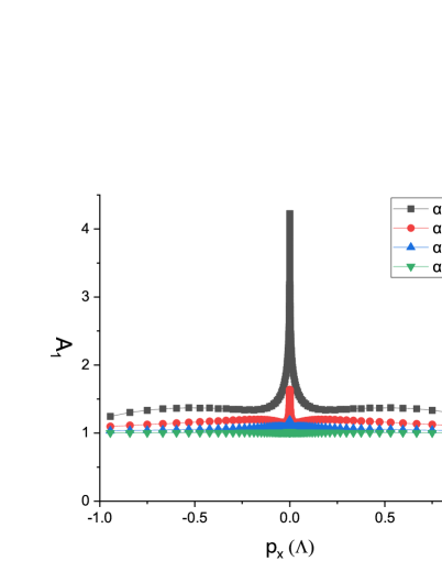
Let us first discuss the behavior of renormalization function $A_{2}(p_{x},p_{y})$. We find it more convenient to consider the momentum dependence of the function $A_{2}(p_{x},p_{y})\beta p^{2}_{y}$, instead of $A_{2}(p_{x},p_{y})$ itself. The full momentum dependence of $A_{2}(p_{x},p_{y})\beta p_{y}^{2}$ obtained by solving Eqs. (32-33) in Fig. 3, for six different values of $\alpha$. It is easy to find that $A_{2}(p_{x},p_{y})\beta p_{y}^{2}$ is nearly independent of $p_{x}$ for small values of $\alpha$. As $\alpha$ exceeds $0.6$, $A_{2}(p_{x},p_{y})\beta p_{y}^{2}$ exhibits a considerable dependence on $p_{x}$. In contrast, $A_{2}(p_{x},p_{y})\beta p_{y}^{2}$ manifests a significant dependence on $p_{y}$ for all values of $\alpha$. To show these properties more explicitly, we plot the $p_{x}$-dependence of $A_{2}(p_{x},p_{y}=0)$ in Fig. 4(a) and the $p_{y}$-dependence of $A_{2}(p_{x}=0,p_{y})$ in Fig. 4(b).

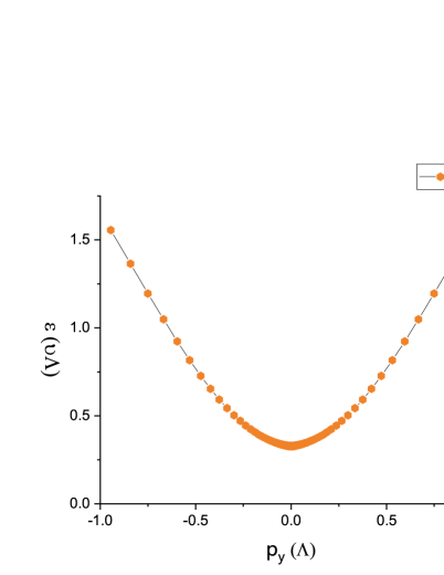
The $p_{y}$-dependence of $A_{2}(p_{x},p_{y})\beta p_{y}^{2}$ deserves a little more analysis. Over a wide range of $p_{y}$ below the UV cutoff, $A_{2}(p_{x},p_{y})\beta p_{y}^{2}$ displays a linear dependence on $p_{y}$. This behavior indicates that the originally quadratic fermion dispersion along the $y$-direction is turned into a linear dispersion owing to the Coulomb interaction. Consequently, the 2D semi-Dirac fermions behave in the same way as the ordinary 2D Dirac fermions that exhibit a linear dispersion along two directions. For small values of $p_{y}$, the dispersion is no longer linear in $p_{y}$. Indeed, a finite energy gap $\Delta_{0}$ is opened at $p_{y}=0$ and such a gap is an increasing function of $\alpha$. The interaction-induced quadratic-to-linear transition of the fermion dispersion along $y$-direction and also the generation of a finite gap have already been obtained previously in the weak-coupling perturbative calculations of Kotov et al.. Kotov21 . Our non-perturbative studies show that these two conclusions remain correct even when the interaction parameter $\alpha$ becomes large.

Summarizing the results shown in Fig. 3 and Fig. 4(b), we find that $A_{2}(p_{x},p_{y})$ can be approximately described by

where $a$ and $b$ are two fitting constants. We assume that $a\gg b$ in the limit of $p_{y}\rightarrow\Lambda$ and that $a\ll b$ in the limit of $p_{y}\rightarrow 0$. For large values of $p_{y}$, the first term dominates over the second term, leading to

For small values of $p_{y}$, the second term dominates such that

where the constant $b\beta$ represents a finite gap. Notice that such a gap does not break any symmetry of the system and persists for an arbitrary weak Coulomb interaction. Its existence implies that the semi-DSM state is unstable against Coulomb interaction and can be easily turned into a BI. However, one can tune this gap to vanish by carefully varying certain external parameters Kotov21 , which then would drive the system to approach the DSM-to-BI QCP. In this regard, the second term of $A_{2}(p_{x},p_{y})$ can be simply dropped, leaving us with only the first term.

The above results show that the function $A_{2}(p_{x},p_{y})\beta p_{y}^{2}$ is linear in $p_{y}$ in the low-energy region. An indication of such a behavior is that the semi-DSM state is actually unstable against the Coulomb interaction since the originally quadratic dispersion along the $y$-direction is strongly renormalized and becomes a linear one. Consequently, the renormalized dispersion of low-energy fermionic excitations of a 2D semi-DSM resembles the cone-shaped dispersion of non-interacting 2D Dirac fermions. By comparing Fig. 2(a) to Fig. 2(b), one can see that the Coulomb interaction renormalizes the dispersions of 2D Dirac fermions and 2D semi-Dirac fermions very differently. Our non-perturbative results qualitatively agree with that obtained by using the first-order weak-coupling perturbative RG method Kotov21 , but appear to be at odds with that obtained by the $1/N$-expansion approach Isobe16 ; Cho16 .

We see from Fig. 4(c) that the renormalization function $A_{1}(p_{x},0)$ is nearly independent of $p_{x}$. Close to the limit of $p_{x}\to 0$, $A_{1}(p_{x},0)$ appears to be substantially enhanced. We emphasize that such an enhancement is actually an artifact of IR cutoff. There is always an IR cutoff for $p_{x}$ in carrying out numerical computations. In our case, the IR cutoff is taken as $10^{-5}\Lambda$. The contributions of the range of $p_{x}<10^{-5}\Lambda$ to $A_{1}(p_{x},0)$ are inevitably neglected. However, as demonstrated in Ref. Pan21 , the long-range nature of the Coulomb interaction indicates that small-momentum contributions are always larger than those of large momenta. If we reduce the IR cutoff, the plateau always extends to lower momentum.

According to the results shown in Fig. 4(d), $A_{1}(0,p_{y})$ is also nearly independent of $p_{y}$ for small values of $\alpha$. But as $\alpha$ grows to fall into the strong-coupling regime, $A_{1}(0,p_{y})$ becomes significantly dependent on $p_{y}$. Based on the above results, we infer that the fermion dispersion remains linear along the $x$-direction within a broad range of $\alpha$ and momentum even when the impact of Coulomb interaction is included.

In Fig. 5(a) and Fig. 5(b), we show how the renormalized fermion spectrum, characterized by the function $\varepsilon(p_{x},p_{y})=\pm\sqrt{A_{1}^{2}(p_{x},p_{y})p_{x}^{2}+A_{2}^{2}(p_{x},p_{y})\beta^{2}p_{y}^{4}}$, depends on $p_{x}$ and $p_{y}$ for a fixed value of $\alpha$, respectively. This spectrum manifests a nearly linear dependence on momentum in both of the two directions within a broad range of $p_{x}$ and $p_{y}$. There seems to be a deviation from the standard linear behavior in the region of small $p_{x,y}$. This deviation stems from the existence of a finite gap at $p_{x,y}=0$. If such a gap is removed by tuning suitable external parameters, the deviation from linear behavior would disappear.

In summary, we have performed a non-perturbative field theoretical study of the renormalization of the dispersion of 2D semi-Dirac fermions by incorporating the influence of long-range Coulomb interaction. Making use of several exact identities, we derive the self-closed DS integral equation of the full fermion propagator and obtain the momentum-dependence of the renormalized fermion spectrum based on the numerical solutions of such an equation. Our results show that the originally quadratic dispersion of semi-Dirac fermions is dramatically renormalized by the Coulomb interaction and changed into a linear one, which is illustrated in Fig. 2(a). However, the originally linear dispersion remains linear after renormalization.

Comparing to the RG approach, the DS equation approach has two major advantages. Firstly, the full momentum-dependence of such physical quantities as the renormalization functions $A_{1}(p_{x},p_{y})$ and $A_{2}(p_{x},p_{y})$ can be obtained from the numerical solutions of their integral equations. In contrast, the RG equations of various model parameters depends merely on a varying scale $l=\ln\left(\Lambda/E\right)$ where $E$ is either the energy or the absolute quantity of the momentum. Secondly, the DS equation of fermion propagator is exact and contains all the interaction-induced effects. Hence the DS equation approach is valid for any values of $\alpha$ and $N$.

In order to simplify numerical computations, we have neglected the energy dependence of the renormalization functions $A_{1}(p_{x},p_{y})$ and $A_{2}(p_{x},p_{y})$. Under such an approximation, the quasiparticle resisue $Z$ cannot be calculated since the renormalization function $A_{0}(p)=1$. Thus the results presented in this paper cannot be used to judge whether the system exhibit non-Fermi liquid behaviors. The computational time of solving the complicated integral equations of $A_{0}(p_{0},p_{x},p_{y})$, $A_{1}(p_{0},p_{x},p_{y})$, and $A_{2}(p_{0},p_{x},p_{y})$ is much longer than that needed to solve the integral equations of $A_{1}(p_{x},p_{y})$ and $A_{2}(p_{x},p_{y})$. We wish to undertake such a task in a future project.

We thank Jing-Rong Wang and Zhao-Kun Yang for helpful discussions. H.F.Z. is supported by the Natural Science Foundation of China (Grants No. 12073026 and No. 11421303) and the Fundamental Research Funds for the Central Universities.

References

- (1) A. H. Castro Neto, F. Guinea, N. M. R. Peres, K. S. Novoselov, and A. K. Geim, Rev. Mod. Phys. 81, 109 (2009).
- (2) V. N. Kotov, B. Uchoa, V. M. Pereira, F. Guinea, and A. H. Castro Neto, Rev. Mod. Phys. 84, 1067 (2012).
- (3) O. Vafek and A. Vishwanath, Annu. Rev. Condens. Matter Phys. 5, 83 (2014).
- (4) M. Hirata, A. Kobayashi, C. Berthier, and K. Kanoda, Rep. Prog. Phys. 84, 036502 (2021).
- (5) R. Shankar, Rev. Mod. Phys. 66, 129 (1994).
- (6) P. Coleman, Introduction to Many-Body Physics (Cambridge University Press, Cambridge, 2015).
- (7) J. González, F. Guinea, and M. A. H. Vozmediano, Nucl. Phys. B 424, 595 (1994).
- (8) D. C. Elias, R. V. Gorbachev, A. S. Mayorov, S. V. Morozov, A. A. Zhukov, P. Blake, L. A. Ponomarenko, I. V. Grigorieva, K. S. Novoselov, F. Guinea, and A. K. Geim, Nat. Phys. 7, 701 (2011).
- (9) D. A. Siegel, C.-H. Park, C. Hwang, J. Deslippe, A. V. Fedorov, S. G. Louie, and A. Lanzara, Proc. Natl. Acad. Sci. U.S.A. 108, 11365 (2011).
- (10) J. Chae, S. Jung, A. F. Young, C. R. Dean, L. Wang, Y. Gao, K. Watanabe, T. Taniguchi, J. Hone, K. L. Shepard, P. Kim, N. B. Zhitenev, and J. A. Stroscio , Phys. Rev. Lett. 109, 116802 (2012).
- (11) X.-Y. Pan, Z.-K. Yang, X. Li, and G.-Z. Liu, Phys. Rev. B 104, 085141 (2021).
- (12) G. Montambaux, F. Piéchon, J.-N. Fuchs, and M. O. Goerbig, Eur. Phys. J. B 72, 509 (2009).
- (13) G. Montambaux, F. Piéchon, J.-N. Fuchs, and M. O. Goerbig, Phys. Rev. B 80, 153412 (2009).
- (14) L.-K. Lim, J.-N. Fuchs, and G. Montambaux, Phys. Rev. Lett. 108, 175303 (2012).
- (15) M. Bellec, U. Kuhl, G. Montambaux, and F. Mortessagne, Phys. Rev. Lett. 110, 033902 (2013).
- (16) P. Dietl, F. Piéchon, and G. Montambaux, Phys. Rev. Lett. 100, 236405 (2008).
- (17) M. O. Goerbig, J.-N. Fuchs, G. Montambaux, and F. Piéchon, Phys. Rev. B 78, 045415 (2008).
- (18) A. Kobayashi, S. Katayama, Y. Suzumura, and H. Fukuyama, J. Phys. Soc. Jpn. 76, 034711 (2007).
- (19) A. Kobayashi, Y. Suzumura, F. Piéchon, and G. Montambaux, Phys. Rev. B 84, 075450 (2011).
- (20) V. Pardo and W. E. Pickett, Phys. Rev. Lett. 102, 166803 (2009).
- (21) V. Pardo and W. E. Pickett, Phys. Rev. B 81, 035111 (2010).
- (22) S. Banerjee, R. R. P. Singh, V. Pardo, and W. E. Pickett, Phys. Rev. Lett. 103, 016402 (2009).
- (23) J. Kim, S. S. Baik, S. H. Ryu, Y. Sohn, S. Park, B.-G. Park, J. Denlinger, Y. Yi, H. J. Choi, and K. S. Kim, Science 349, 723 (2015).
- (24) B. Wunsch, F. Guinea, and F. Sols, New. J. Phys. 10, 103027 (2008).
- (25) L. Tarruell, D. Greif, T. Uehlinger, G. Jotzu, and T. Esslinger, Nature 483, 302 (2012).
- (26) H. Isobe, B.-J. Yang, A. Chubukov, J. Schmalian, and N. Nagaosa, Phys. Rev. Lett. 116, 076803 (2016).
- (27) G. Y. Cho and E.-G. Moon, Sci. Rep. 6, 19198 (2016).
- (28) V. N. Kotov, B. Uchoa, and O. P. Sushkov, Phys. Rev. B 103, 045403 (2021).
- (29) J. M. Link, B. N. Narozhny, E. I. Kiselev, and J. Schmalian, Phys. Rev. Lett. 120, 196801 (2018).
- (30) J.-R. Wang, G.-Z. Liu, and C.-J. Zhang, Phys. Rev. B 95, 075129 (2017).
- (31) B. Uchoa and K. Seo, Phys. Rev. B 96, 220503(R) (2017).
- (32) M. D. Uryszek, E. Christou, A. Jaefari, F. Krüger, and B. Uchoa, Phys. Rev. B 100, 155101 (2019).
- (33) B. Roy and M. S. Foster, Phys. Rev. X 8, 011049 (2018).
- (34) G.-Z. Liu, Z.-K. Yang, X.-Y. Pan, and J.-R. Wang, Phys. Rev. B 103, 094501 (2021).