FemtoDet: An Object Detection Baseline for Energy Versus Performance Tradeoffs
Abstract
Efficient detectors for edge devices are often optimized for parameters or speed count metrics, which remain in weak correlation with the energy of detectors. However, some vision applications of convolutional neural networks, such as always-on surveillance cameras, are critical for energy constraints. This paper aims to serve as a baseline by designing detectors to reach tradeoffs between energy and performance from two perspectives: 1) We extensively analyze various CNNs to identify low-energy architectures, including selecting activation functions, convolutions operators, and feature fusion structures on necks. These underappreciated details in past work seriously affect the energy consumption of detectors; 2) To break through the dilemmatic energy-performance problem, we propose a balanced detector driven by energy using discovered low-energy components named FemtoDet. In addition to the novel construction, we improve FemtoDet by considering convolutions and training strategy optimizations. Specifically, we develop a new instance boundary enhancement (IBE) module for convolution optimization to overcome the contradiction between the limited capacity of CNNs and detection tasks in diverse spatial representations, and propose a recursive warm-restart (RecWR) for optimizing training strategy to escape the sub-optimization of light-weight detectors by considering the data shift produced in popular augmentations. As a result, FemtoDet with only 68.77k parameters achieves a competitive score of 46.3 AP50 on PASCAL VOC and 1.11 W 64.47 FPS on Qualcomm Snapdragon 865 CPU platforms. Extensive experiments on COCO and TJU-DHD datasets indicate that the proposed method achieves competitive results in diverse scenes.
1 Introduction
The deployment of efficient convolutional neural networks (CNNs) enabled immense progress [24, 30, 31, 32, 4, 10, 43] in vision detectors for edge devices, in which they consistently reduce parameters and speed counts for improving accuracy. However, these metrics are not correlated well with the efficiency of the models in terms of energy. Evaluation metrics, such as parameters, do not take into account the energy cost of models, resulting in a nontrivial effect on the energy cost of detectors. Compared with the same architecture, the parameters of models are positively correlated with their energy cost (shown in Table 2). However, in the case of equal model parameters, their energy consumption may be negatively correlated or even irrelevant to the model parameters (shown in Table 1). Considering that various activation functions, convolution operators, and feature fuse structures may not increase model parameters, but generate more energy costs. Similarly, the speed count is also not well correlated with energy, as it can be optimized by the degree of parallelism. These disconnections will leave customized efficient detectors unavailable, when they are deployed under severe energy constraints like the always-on surveillance cameras.
This paper aims to reduce the energy costs of efficient object detectors, while improving their performances by achieving energy versus performance tradeoffs. Specifically, these bottlenecks fall into several categories:
1) Detector components with unknown energy. Most current object detection methods focus either on latency-oriented [5, 35, 46] or accuracy-oriented [10, 39, 33, 37] works. There are very limited works toward the energy cost of the detector components, which is the first obstacle to designing energy-performance-balanced detectors. To identify energy-efficient components of detectors, we followed [44] to benchmark their energy metrics from three types of structures, i.e., activation functions, convolution operators, and necks of detectors. The following finding is acquired: Firstly, some activation functions have been widely used, because of their ability to improve models without adding more parameters. They have increased costs, yet received very limited attention. As shown in Table 1, we set ReLU [1] based models as a baseline. When replacing the ReLU with the GELU [17], 4.40% performance is gained, while 12.50% energy cost is increased, and the corresponding factor of the mean energy versus the performance tradeoffs (Eq. 1) drops 7.16%. In addition, although large kernel convolutions [26] can improve models (Table 2), the increased energy cost is unacceptable. As seen in Table 2, the large kernel convolutions are equipped to enable the model to rise by around 1.87% in performance, but with more energy costs (16.20%) than in the small kernel size of convolutions (shown in the second row of Table 2). Finally, the standard FPN [22, 23, 41, 11, 38] in the detectors also causes significant energy costs. We observe that this situation is happened due to multi-feature fusion paths following either bottom-to-up or top-to-down way, resulting in frequent data reading in memory for data coverage. However, it is shown that the up-down fusion between multi-features may not necessary. As shown in Table 3, we propose a simple SharedNeck for replacing FPN to reduce around 5.77% energy costs, while obtaining 6.25% performance gains. SharedNeck uses an adaptive fusion between multi-features by learning convolution, instead of feature-by-feature bottom-to-up or top-to-down fusions, as operated in FPN. Based on these analyses, we further build upon a low-energy detector, named FemtoDet. Surprisingly, FemtoDet just has 68.77k parameters and 1.1W power on the platform. 2) Optimization for CNN is another bottleneck, since obtaining a favorable detector is very challenging, especially for a small number of parameters. Light-weight detectors are restricted by their limited capacities [6], which will cause obfuscation on feature maps of the instances’ boundaries of interesting objects, as shown in Figure 2 (b). Ambiguous instance boundaries on the features may raise the risk of false detection in the models. For this problem, we propose a novel instance boundary enhancement module (IBE), which emphasizes the potential of the object boundary information: The parameter reuse mechanism is first applied to integrate local descriptors with convolution operation to make robust and diverse instance boundary feature representation. But this operation would cause feature un-alignment between normal features and integrated features. Then, in order to sufficiently exploit these two types of features, we design dual-normalization in IBE, as to re-align the features (Fig. 4 of the Appendix). IBE employs a shared convolution yet an independent batch normalization layer for separate normalization is also adopted. Finally, we add normal and integrated features together behind the dual-normalization layer. IBE provides a novel form of parameter reuse to generate new local descriptors from shared convolution operators. This method can capture object boundary information by integrating gradient cues around the learned convolution. After trained, IBE modules can be folded into simple convolution operators, thus requiring no extra computations anymore; In addition, data augmentation is a common approach for efficient detector training. Using well-designed strong augmentations is conducive to improving the generalization of models [32, 10]. However, how to prevent data shifts between training and validation images has not been explored, while training data suffers strong augmentations. It is found that the produced data shifts by strong augmentations would prevent light-weight detectors from moving toward global optimization. A common view is that strong image augmentations can effectively encourage networks to learn diverse features [12]. But for light-weight detectors, these diverse features cannot assist the models in making better generalizations in the validation set. In other words, light-weight detectors are more susceptible to these ignored data shifts because of their limited capacities. Furthermore, we propose an effective training strategy, namely recursive warm-restart (RecWR), to adapt these diverse features to improve the model’s generalization. RecWR works based on multi-stage training while gradually weakening data augmentation strength. This method can help the limited-capacity detectors jump out of local optima under the assistance of high-dimension diverse features. The effectiveness of the IBE and RecWR has been evaluated on PASCAL VOC dataset. And the experimental results show that IBE can improve FemtoDet performance, while incurring no extra parameter burdens, as compared to the original architecture; RecWR can improve FemtoDet performance by gradually weakening the data augmentation strength in multi-stage learning. By jointly training FemtoDet with IBE and RecWR, our proposed methodology can go over the YOLOX [10] by in performance when using the same-level parameters.
Something worth mentioning is that FemtoDet is specially designed for hierarchical intelligent chips to enable always-on alerts: the always-on low power, high-recall, and decent accuracy - it achieved 85.8 AR20 76.3 AP20 (Table 7) while performing pedestrian detection on TJU-DHD. In addition, FemtoDet is poor in detecting small objects but is excellent in detecting medium and large objects, which they are more interested in, with 88.8 AR20-m 94.1 AP20-m / 95.3 AR20-l 98.6 AP20-l (Table 7) on TJU-DHD. Information can be passed to other models after identifying possible objects of interest, and high-precision robust models are then initiated for accurate recognition. The always-on smart products have a wide range of applications, e.g., in-home monitoring or robots. Hence, the loose metric (e.g., AP50 or AP20) and data scenario with moderate difficulty (e.g., VOC) can well reflect the application ability of FemtoDet. Further, the experiments on COCO datasets have verified that the proposed method is suitable for diverse scenarios resulting in competitive results.
2 Related Works
2.1 Object Detection
Object detection is a classic computer vision task for identifying the category and location of object in pictures or videos. The existing object detectors can be divided into two categories: two-stage detectors and one-stage detectors. Two-stage detectors [33, 37, 15, 22] are anchor-based devices that generate region proposals from the image and then produce the final prediction boxes from these proposals. Further, FPN [22] improves the two-stage detectors by fusing multi-level features. Despite their higher accuracy compared to the one-stage detectors, two-stage detectors are still difficult to achieve low latency when deployed on edge devices.
Specifically, there are two types of one-stage detectors: anchor-based and anchor-free, which depends on anchor priors injecting into whole images to enable box regression. SSD [24], as a classical anchor-based one-stage detector, discretizes the output space of bounding boxes into a set of default anchors with different aspect ratios and scales per feature map location. This operation helps detecting tiny objects. Another typical anchor-based detector is the YOLO series [31, 32, 4]. YOLOv2 [31] explores bag of freebies to improve the performances of one-stage detectors. YOLOv3 [32] proposes cross-scale features and novel nms (Non-Maximum Suppression) to obtain more confident predictions. YOLOv4 [4] finds that the repeated gradient of network optimization aggravates detector latency, and thus designs Cross-Stage-Partial-connection modules to reduce the latency of detectors while maintaining detection performance. Anchor-free detectors [30, 10, 20, 39] aim to eliminate the pre-defined set of anchor boxes. YOLO [30], as an anchor-free one-stage detector, divides an image into multiple grids and predict boxes at grids near the object’s center. CornerNet [20] detects an object as a pair of key points (through the top-left corner and bottom-right corner of the bounding box). A single convolutional network was leveraged in CornerNet to predict a heatmap for all top-left corners of instances of the same object category, a heatmap for all bottom-right corners, and an embedding vector for each detected corner. Indeed, CornerNet is a new pipeline for object detection. FCOS [39] eliminates the anchor setting by proposing a fully convolutional one-stage object detector, which can solve object detection in a per-pixel prediction manner. The anchor-free detectors solve the problem happened in anchor-based detectors, which reduce the memory cost and increase accuracy of the bounding box.
Both one-stage and two-stage object detection methods have obtained high performance on many challenging public datasets, i.e., COCO and TJU-DHD [28]. These methods provide the accuracy-oriented detectors. However, the critical problem for detectors serving edge devices is detection latency and its power. In other words, detectors obtain higher performance in challenging scenes, which is not a necessary option for detectors deployed on edge devices. For the detection latency, a lot of effort [5, 35, 46] have been devoted to achieving the balance between accuracy and efficiency. FastYOLO [35] is an optimized architecture extended from YOLOv2 with fewer parameters and performance drop, which makes FastYOLO run at an average of 18FPS on an Nvidia Jetson TX1 embedded system. YOLObite [5] focuses on pruning redundancy object detectors to be real-time by designing in a compression-compilation way. NanoDet uses ShuffleNetV2 [27] as its backbone to make the model lighter, and further uses ATSS [50] and GFL [21] to improve its accuracy. It is worth noting that NanoDet also reached 60FPS on an ARM CPU. These light-weight detectors are latency-oriented. Actually, neither accuracy-oriented nor latency-oriented detectors take their energy cost into account. High energy cost detectors are unfriendly to devices deployed at edges.
This paper aims to develop a light-weight detector that can achieve tradeoffs between energy and performance.
2.2 Energy-Oriented Convolutional Neural Networks
Besides the manual design of deep neural networks, a great deal of work has been done to improve the effectiveness and efficiency of deep neural networks via network pruning [47], quantization [14, 2], architecture search [13, 42]. ECC [44] proposes the end-to-end classifier training framework, which provides quantitative energy consumption guarantees by using weighted sparse projection and input masking. Zhang [49] specialized in video broadcast and leveraged distillation techniques to reduce memory consumption by approximating the video frame data. MIME [3] is an algorithm-hardware co-design approach that reuses the weight parameters of a trained parent task and learns task-specific threshold parameters for inferring on multiple child tasks. However, the above works are all in service for image classification, and we can observe that fewer parameters represent lower energy costs in the same architecture. Object detection on edge devices is still a challenging topic, considering that the conflict between the limited capacity of CNNs and diverse spatial representations. This paper is the first work to provide a systematized solution for energy-oriented light-weight detectors.
3 FemtoDet
This section will be divided into two subsections to describe how FemtoDet achieves energy versus performance tradeoffs. 1) Benchmarks for Low-energy Detectors: We provide benchmarks for designing low-energy detectors, including the exploring of activation functions, convolution operators, and neck of detectors. 2) Energy-Oriented FemtoDet: Based on the benchmarks for designing low-energy detectors, an energy-oriented light-weight detector named FemtoDet is provided, which stacks layers from depthwise separable convolutions (DSC), BN and ReLU. FemtoDet involves only 68.77k parameters and power of 1.11W on the Qualcomm Snapdragon 865 CPU platform. Moreover, FemtoDet can be optimized with two designs: Firstly, instance boundary enhancement (IBE) modules are used to improve the DSC in FemtoDet, overcoming the bottleneck of light-weight models’ representation optimization (i.e., models will learn obfuscation features because of their limited capacity, as shown in Fig. 2 (b)). Second, the recursive warm-restart (RecWR) training strategy is a multi-stage recursive warm-restart learning procedure, which can surmount data shifts produced from strong data augmentations.
3.1 Benchmarks for Low-energy Detectors’ Designing
3.1.1 Evaluation Metrics
Top1-Acc (top1 accuracy, for image classification), and AP (average precision, for object detection) are widely used measures to evaluate the performance of CNN. In addition to the commonly used metrics and , we propose the (energy costs) and (mean energy versus performance tradeoffs) to comprehensively evaluate the energy costs of the models and their ability to achieve energy versus performance tradeoffs. Specifically, and are represented by
| (1) |
| (2) |
where indicates the total times required to evaluate images, represents the energy costs while models evaluate -th image with trained parameters . is similar to . The difference is that we set a value of 1 for each layer of channels, where the model parameter is . indicates that the model is an empty state. denotes the model performance (top1-Acc for image classification while evaluating activation functions and convolution operators, AP50 for object detection while evaluating necks of detectors in Sec. 3.1.2) in image . For the power metric, the value is expected to be as small as possible. For the mEPT metric, the result is expected as greater as possible.
3.1.2 Components to Be Evaluated
To identify low-energy components of detectors, we followed [44] to benchmark their energy costs from three types of structures: activation functions, convolution operators and necks of detectors:
Activation Functions. Rectified Linear Unit (ReLU) [30, 24], GELU [17], Swish [10], SiLU [9], and etc. are widely used for object detection because they have fewer parameters and flops. We calculate the energy costs of different activation functions in the same architecture to explore which activation function is more friendly for designing an energy-oriented detector.
Convolution Operators can automatically learn filer weights while CNNs are trained to summarize helpful information, including horizontal, vertical, edged, diagonal, and etc. features from images. Vanilla convolutions (vanConv) [19], depthwise separable convolutions (DSC) [18] and their large kernel size versions [26] are widely used. Ding et al. [8] pointed out that when CNNs are constructed based on enough large convolution kernels, results can be comparable to the transformer [25]. Here, we set up energy consumption comparison experiments with different convolutions (vanCon and DSC) and multi-scale convolution kernel sizes (33, and 55) on different network structures (ResNet and MobileNetV2). It is important that for each experiment case, the convolution operator type or kernel size would be the only variable.
Necks of Detectors: Feature pyramid networks (FPN) are essential components for two-stage or one-stage detectors. FPN-based necks of detectors fuse multiple low-resolution and high-resolution feature inputs for better representations, leading to a series of studies for designing manually complex fusion methods [22, 23, 41]. However, they only presented favorable results brought by FPN but ignored its energy costs. We form a series of experiments on FemtoDet by using different neck types, e.g. FPN [22], PAN [23], and our proposed SharedNeck (details can be found in Sec. 3.2.1) to study corresponding metrics (including energy costs, parameters, and detection precision on PASCAL VOC) changes.
All related experiments can be found in Sec. 4.1. We can observe that DSC and ReLU are more energy friendly than vanCon and other activation functions. In addition, by comparing with the necks of detectors such as FPN and PAN, the proposed SharedNeck is more suitable for light-weight detectors.
3.2 Energy-Oriented FemtoDet
3.2.1 Building FemtoDet
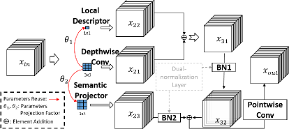
Backbone: The backbone of FemtoDet contains an initial full convolution layer with 8 filters. We use ReLU as the non-linearity and BN as the batch normalization. From the second layer beginning, all the convolution operators use DSC. The reason is that we follow the results of our benchmarks (the results can be seen in Sec. 4.1) to select the energy friendly components. The whole backbone is described in Appendix Table 9; Neck: We customize a neck for FemtoDet to achieve better tradeoffs between energy and performance. In detail, SharedNeck first aligns the scale information of inputs from backbones, and then merges these alignment features with elements addition. Finally, a DSC performs adaptive multi-scale information fusion between merged features. The implementation details of SharedNeck, and how it differs from other necks are shown in Fig. 1; Head and Training Loss: Here, we use the decouple head of YOLOX as the head of our proposed detector with the same training loss as YOLOX.


3.2.2 Instance Boundary Enhancement Module
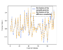
Optimizing light-weight detectors is a notoriously challenging problem. The reason for this is that limited by their representation, features learned by detectors are diffuse, as shown in Fig. 2 (b). Instance boundary enhancement (IBE) modules are designed to improve the DSC in FemtoDet, thus overcoming the bottleneck of light-weight models’ representation optimization. IBE is similar to modules introduced in [47, 36, 45], except that our modules are designed for convolutional layers that are factorized into depthwise and pointwise layers. We further introduce a dual-normalization mechanism, such that the IBE modules can be used for object detection, while the modules in [47, 36, 45] just working for low-level tasks. Based on the DSC block, the basic block of IBE includes 33 depthwise convolution followed by 11 convolution. IBE enhances DSC by designing a new local descriptor, semantic projector, and dual-normalization layer. Specifically, the 11 local descriptor is a parameter reusing mechanism generated by the linear transformation of the integrating gradient cues around shared depthwise convolution. Therefore, the object boundary information can be found in the local descriptors. Previously, the local descriptor is known as the difference convolution [47, 36, 45] used for low-level tasks. Although the idea is easy to get that using these object boundary information to enhance the noisy feature representation (shown in Fig. 2 (b)) of the above standard operators, such as depthwise convolution, in practice, the original difference convolution architecture cannot serve for high-level semantic tasks. We observe that features obtained by the difference convolution are unaligned with the features obtained by standard convolution (the figure shown in Fig. 4 of the Appendix). On the one hand, the difference convolution captures diverse information about object boundaries by integrating gradient cues around 33 or with larger convolution. On the other hand, high-level tasks encourage standard convolution to summarize the abstract semantic information of images. That is the reason that the classical difference convolution cannot serve high-level tasks. To simultaneously solve this problem, we propose a semantic projector and a dual-normalization layer. The semantic projector is the linear transformation of depthwise convolution to transfer operators related to semantic information extraction; The dual-normalization layer consists of two independent batch normalization modules specifically designed for aligning the unaligned features. After that, we incorporate the object boundary cues from the feature addition between the local descriptor and depthwise convolution to guide the model in learning an effective representation of the instance (refined results can be seen in Fig. 2 (c)).


The description of IBE modules is given in Fig. 3 of the Appendix. For the depthwise convolution of kernel size 3, denotes the input channel dimension, represents the output channel dimension, the weight matrix can be denoted as , and the bias is represented as . The local descriptor of kernel size 1 can be generated from the depthwise convolution by reusing parameters. Its weight matric is denoted as , which is integrating the gradient cues around :
| (3) |
where , is a learnable parameter projection factor. represents the convolution in , and is the -the weight value. Integrating the gradient cues around can help the local descriptors capture the object boundary information effectively. The semantic projector is generated from the depthwise convolution, while diverse semantic presentations can be obtained through a learnable linear transformation, shown as follows:
| (4) |
where is another learnable parameter as the projection factor. Subsequently, the IBE modules perform four steps to refine the feature representation under the guidance of object boundary information. 1) inputs will be convolved with the obtained three convolution operators, and the corresponding results are denoted as , and , respectively; 2) elements addition are conducted between and ; 3) the dual-normalization layer enables feature distribution normalization on and ; 4) the two outputs from the dual-normalization layer can be added together; As a result, the aforementioned added features are convolved through pointwise convolution as the final output of the IBE module.
In addition, we leverage the homogeneity and additivity of the convolutions to fold IBM modules into the simpler depthwise separable convolution in the inference stage without performance degradation. The details can be seen in Appendix C.
3.3 Recursive Warm-restart Training Strategy
Strong augmentations (SA) are widely used for object detection, and [10, 32] shows well-designed SA effectively improves detectors. However, we find that well-designed SA does not always benefit light-weight detectors, because the current training strategies cannot sufficiently exploit diverse training representations to boost the generalization ability on real validation data. For example, YOLOX [10] points out MixUp reduces YOLOX-nano’s performance by about 5. We argue that the limited capacity detectors fit the diverse data generated by SA as much as possible during training, such that the modules have no surplus capacity to adjust learned features to boost the generalization ability of modules on real validation data. In other words, SA produces diverse representations that are equal to the data shifts, thus breaking the generalization ability of the module. We also propose an effective training strategy to adjust these diverse features to improve the generalization ability, namely recursive warm-restart (RecWR).
As shown in Fig. 5 of the Appendix, the whole training procedure can be divided into four stages. Starting from the 1- stage to 4- stage training, the intensity of image augmentations gradually decreases. Specifically, in the 1- training stage, some SA types will be combined, such as MixUp, Mosaic, and RandomAffine. Starting from the 2- training stage, the above SA types are gradually unloaded in each training stage, until the 4- training stage. For the last training stage, only the random flip and random scales are performed on the training data. In addition, before starting each training stage, the waiting training detectors load the trained weights of the previous training stage as the initialization.
We can see that in Appendix D, after training FemtoDet with RecWR, MixUp also help such extremely small detectors obtain better performance. In other words, RecWR takes advantage of diversity features learned from SA to get FemtoDet out of sub-optimization.
4 Experiments
We used VOC, COCO, TJU, and ImageNet datasets to conduct experiments and validate the proposed method. Specifically, whole experiments can be divided into two sections, , identifying low-energy components of detectors mentioned in Sec. 3.1.2, and validating the effectiveness of our designed FemtoDet, where the metric was measured in GTX 3090.
| Activation | Param | Power | Top1 | mEPT |
| Functions | (M) | (W) | (Acc) | |
| ReLU [1] | 1.48 | 5.04 | 45.22 | 8.97 |
| GELU [17] | 5.67 | 47.21 | 8.33 | |
| Swish [10] | 5.47 | 47.45 | 8.67 | |
| HSwish [46] | 5.33 | 47.60 | 8.93 | |
| SiLU [9] | 5.73 | 47.25 | 8.25 |
4.1 Benchmark to Find Low-energy Components
4.1.1 Activation Functions
Table 1 shows the energy-related metric results using different activation functions under the same architecture (MobileNetV2 0.25). We observe that the activation functions can significantly improve models without extra parameters (Param). On the other hand, such activation functions incur unacceptable overhead on some metrics which are inconvenient to measure. For example, Swish improves ReLU-based models performance by 4.93, but produces more than 8.53 more energy cost. The mEPT metric also demonstrate that ReLU results in the best energy versus performance tradeoffs.
| CNNs | Convolution | Param | Power | Top1 | mEPT |
|---|---|---|---|---|---|
| Operators | (M) | (W) | (Acc) | ||
| Res18 | 12.46 | 170.64 | 69.93 | 0.41 | |
| 31.99 | 198.28 | 71.24 | 0.36 | ||
| MBV2 | 2.29 | 5.56 | 69.51 | 12.50 | |
| 2.35 | 6.07 | 70.96 | 11.69 |
4.1.2 Convolution Operators
This sub-section compares energy-related metrics while training an image classifier on the ImageNet dataset based on the different convolution operators (vanCon and DSC), and the different kernel sizes (33, and 55) on the same convolution operator. Experimental results in Table 2 shows that: 1) When CNNs were constructed with the same kernel size, mobilenetv2 generated much lower energy costs than resnet18, as shown in Table 2 of and . In other words, DSC is more energy friendly than vanConv while achieving similar performance; 2) When CNNs were constructed with different kernel sizes and the same types of operators, the smaller kernel generated much lower energy costs than the larger kernel, as shown in Table 2 of and . However, the performance gain from the large kernels is not so impressive.
4.1.3 Necks of Detectors
Here we evaluated the effects of different necks (including FPN, PAN, and SharedNeck) in FemtoDet. Experimental results are shown in Table 3, and some observation are summarized as follow: 1) Although FPN enables FemtoDet to achieve preferable results, it not only consumes more energy but also has a large parameter overhead; 2) Due to the limited representation of light-weight models, the top-down and bottom-up feature fusion of PAN is poor; 3) SharedNeck achieves the best results in the metrics of parameter, energy cost, object detection performance, and factors of mean energy versus performance tradeoffs by performing adaptive feature fusion.
| Necks of Detectors | Param | Power | AP50 | mEPT |
| (k) | (W) | |||
| FPN | 176.31 | 8.31 | 40.04 | 4.82 |
| PAN | 79.83 | 7.97 | 39.91 | 5.01 |
| SharedNeck | 69.77 | 7.83 | 42.50 | 5.43 |
| Methods | Param | Power | AP50 | mEPT |
| (k) | (W) | |||
| YOLOX | 70.39 | 10.42 | 30.60 | 2.94 |
| NanoDet Plus | 69.60 | 11.29 | 38.44 | 3.40 |
| FemtoDet | 68.77 | 7.83 | 46.31 | 5.91 |
| Methods | mAP | mAP-s | mAP-m | mAP-l |
| YOLOX | 13.60 | 3.00 | 5.10 | 16.60 |
| NanoDet Plus | 20.78 | 4.02 | 8.07 | 25.48 |
| FemtoDet | 22.90 | 1.10 | 8.40 | 28.50 |
| Methods | Param (k) | AP50 | Inference | |
| Power (W) | FPS | |||
| YOLOX | 70.39 | 30.60 | 1.41 | 38.04 |
| NanoDet Plus | 69.60 | 38.44 | 1.37 | 47.80 |
| FemtoDet | 68.77 | 46.31 | 1.11 | 64.47 |
4.2 Validating the Effectiveness of FemtoDet
We verify the effectiveness of FemtoDet on three datasets: PASCAL VOC, COCO, and TJU-DHD, while resizing inputs to 640640 for training and resizing inputs to 416416 for validating. Two datasets, PASCAL VOC and TJU-DHD two datasets are converted to the COCO data types for evaluation. In addition, we extract campus data from the TJU-DHD dataset to evaluate the pedestrian detection performance of our proposed extremely light detector, , FemtoDet. Considering extremely light-weight detectors are challenging to fit the complex COCO dataset with poor detection performance, we pull the corresponding results to Appendix E. Also, we compare the detection performance of FemtoDet with YOLOX, and NanoDet Plus [29], in which they are at the same parameter level to ensure fairness. All the detector backbones are pretrained on the ImageNet for 100 epochs, and the metric of mEPT presented in this section is calculated between AP50 and Power.
4.2.1 Results on PASCAL VOC
Experimental results are presented in Table 4, which shows light-weight detectors with eight metrics: parameter (Param), energy cost (Power), AP50, factors of mean energy versus performance tradeoffs (mEPT), mAP, mAP of small size objects (mAP-s), mAP of medium size objects (mAP-m), and mAP of large size of objects (mAP-l) respectively. We can see that although YOLOX has a large number of parameters, it is much lower than FemtoDet in many metrics. NanoDet Plus has the parameter comparable to that of FemtoDet, but only outperforming FemtoDet in the metrics of mAP-s. We believe that for such extremely light-weight detectors, their performances on large-scale objects are the most critical. FemtoDet also presented better results than YOLOX and NanoDet Plus on the metrics of mAP-l. Although the metrics mEPT, used to evaluate performance and energy balance, FemtoDet achieves the best balance compared to the other two models.
In addition, we evaluated the inference speed (FPS) and power of trained detectors on Qualcomm Snapdragon 865 CPU platforms. As shown in Tab. 5, our FemtoDet also achieves the smallest energy costs and inference speed on edge devices.
| Methods | Param | Power | AP50 | mEPT |
| (k) | (W) | |||
| YOLOX | 67.37 | 9.85 | 59.40 | 6.03 |
| FemtoDet | 67.54 | 6.92 | 66.90 | 9.67 |
| Methods | mAP | mAP-s | mAP-m | mAP-l |
| YOLOX | 29.00 | 11.50 | 37.60 | 54.20 |
| FemtoDet | 33.10 | 17.60 | 50.20 | 61.50 |
| Methods | Param | Power | AR20 | AP20 |
| (k) | (W) | |||
| YOLOX | 67.37 | 9.85 | 90.40 | 42.10 |
| FemtoDet | 67.54 | 6.92 | 85.80 | 76.30 |
| Methods | AR20-m | AP20-m | AR20-l | AP20-l |
| YOLOX | 83.70 | 34.80 | 96.10 | 55.60 |
| FemtoDet | 94.10 | 88.80 | 98.60 | 95.30 |
4.2.2 Results on TJU-DHD
Extremely light-weight detectors like FemtoDet have broad application prospects in surveillance scenarios. Hence, we evaluate the performance of FemtoDet in pedestrian detection using the campus dataset of TJU-DHD, and show the performance of the detectors on the less stringent metric AP20. Table 6 and 7 demonstrate that FemtoDet is competent for pedestrian detection in common surveillance scenarios: 1) FemtoDet has lower energy costs in deployment, which is 29.74 lower than YOLOX; 2) FemtoDet obtains 76.3 AP20, while YOLOX with the same parameters only obtain 71.80 AP20.
| IBE | RecWR | 300e | 1200e | AP50 | |
|---|---|---|---|---|---|
| FemtoDet* | ✗ | ✗ | ✔ | ✗ | 42.50 |
| ✗ | ✗ | ✗ | ✔ | 42.11 | |
| ✗ | ✔ | ✗ | ✗ | 45.13 | |
| ✔ | ✗ | ✔ | ✗ | 45.78 | |
| ✔ | ✔ | ✗ | ✗ | 46.31 |
4.2.3 Ablation Studies
We conduct a series of ablation studies on PASCAL VOC to demonstrate the effectiveness and efficiency of our IBE modules and RecWR training strategy. As shown in Table 8: 1) The second and third rows present that by training with 300 and 1200 epochs for FemtoDet*, such a longer epochs do not yield better gains. 2) The fourth and fifth rows present FemtoDet* was trained with RecWR and 300 epochs with the enhancement of IBE, respectively. Results show that independently equipping IBE and RecWR can improve model performance. 3) The six rows demonstrate that jointly using IBE and RecWR enables FemtoDet to achieve the best performance.
5 Conclusion
This paper presented a baseline to encourage the research on energy and performance balance detectors. Our experimental results clearly showed that boosting performance can also cause problem of growth in energy consumption. Conversely, the simple components like ReLU are suitable for building energy-oriented detectors. In addition, we also proposed a novel IBE module and RecWR training strategy to overcome the optimization problem of extremely light-weight detectors. Compared to other state-of-the-art methods under the same parameters setting, IBE and RecWR support these baselines achieving the best performance on VOC, COCO, and TJU-DHD datasets, while consuming the least energy. In the future, we will continue improving the detectors on the balance of energy and performance.
Appendix
Appendix A Training Settings
Appendix B Architecture Details of the Backbone
Table 9 presents the details of FemtoDet’s backbone, which consists of 1 vanilla convolution and 13 depthwise separable convolutions (DSC).
| Input | Operator | ||||
|---|---|---|---|---|---|
| vanConv | - | 8 | 1 | 2 | |
| DSC | 1 | 8 | 1 | 1 | |
| DSC | 4 | 8 | 2 | 2 | |
| DSC | 4 | 8 | 2 | 2 | |
| DSC | 4 | 16 | 3 | 2 | |
| DSC | 4 | 24 | 2 | 1 | |
| DSC | 4 | 40 | 2 | 2 | |
| DSC | 4 | 80 | 1 | 1 | |
| DSC | - | - | - | - |


Appendix C Folding IBE to be DSC When Inferencing
According to the overview of IBE shown in Fig. 3, we represent the depthwise convolution, pointwise convolution, local descriptor, and semantic projector as , , , and respectively. The output features of can be obtained by , where , . According to the homogeneity and additivity of the convolutions [7], we then show the process of folding all above complex operations into the depthwise convolution:
1) Merging the and . First, we express the weight matrix and bias of the as and , the variate of the as , , and . Then, we have , . Finally, we obtain a new convolution , which the weight matrix and bias of which is , . In other words, the two-step operation is equivalent to the one-step operation ;
2) Fold to once convolution operation. First, based on the homogeneity of the convolutions, we can convert the multiplication between the constants and features to that between constants and convolution operators. That means . And the weight matrix and the bias of the new convolution are and , respectively. Second, according to the additivity of the convolutions, we can convert the addition between features to that between convolution operators. The can be re-write as . Where and denotes the weight matrix and bias of , and is the weight matrix and bias of , and () and () indicates the weight matrix and bias of ;
3) Similar to 1), can be merged into a new convolution as ; Like 2), can be folded to be a single convolution operator. After all the above operations, we can fold IBE to be DSC when inferencing.
Appendix D Explore the Impact of MixUp on Training FemtoDet
| RecWR | 300e | AP50 | |||
|---|---|---|---|---|---|
| FemtoDet | ✔ | ✗ | ✗ | ✗ | 46.31 |
| ✗ | ✔ | ✗ | ✗ | 45.79 | |
| ✗ | ✗ | ✔ | ✗ | 42.50 | |
| ✗ | ✗ | ✗ | ✔ | 36.00 |
Table 10 shows the impact of MixUp [48] on training FemtoDet: 1) The second and third rows present the process of training FemtoDet with RecWR and , demonstrating that might MixUp can help light-weight detectors achieve better performance when combined with RecWR; 2) The fourth and fifth rows show that MixUp hurts the light-weight detectors in the standard training strategy, which is consistent with the given by YOLOX; 3) Combining 1) and 2), we conclude that MixUp can only improve the light-weight detectors if it is used for light-weight detectors training under the RecWR. In other words, RecWR takes advantage of diversity features learned from MixUp to get light-weight detectors out of sub-optimization.
Appendix E Results on COCO
| Methods | Param | Power | AP50 | mEPT |
| (k) | (W) | |||
| YOLOX | 79.93 | 11.58 | 9.50 | 0.82 |
| NanoDet Plus | 72.66 | 12.80 | 11.79 | 0.92 |
| FemtoDet | 72.67 | 8.28 | 12.60 | 1.52 |
| Methods | mAP | mAP-s | mAP-m | mAP-l |
| YOLOX | 4.50 | 0.70 | 3.70 | 7.90 |
| NanoDet Plus | 6.54 | 1.72 | 5.75 | 10.39 |
| FemtoDet | 6.20 | 0.70 | 6.00 | 11.00 |
COCO is another widely used object detection dataset with much greater, data complexity than PASCAL VOC. This dataset contains 80 categories of around 160K images collected from the web. We train detectors on the train2017 with 118K images and validate detectors on the val2017 with 41K images. Table 11 compares the performance of YOLOX and FemtoDet on COCO. Results on the metrics of detection seem terrible. The reason is that detectors are too light-weight to accommodate such complex data. Even so, FemtoDet performs better on COCO than YOLOX.
Appendix F Why is the IBE module able to capture the object boundary information?
Classical edge detection [40, 51] identifies sharp image brightness changes such as discontinuities in intensity, colour, or texture; image gradients or derivatives information are the first choices to extract such information. Two perspectives enable IBE to capture the object boundary information: 1) First, the local descriptor is established to explore image gradient cues by integrating gradients around depthwise convolution; 2) Second, the different convolutions in IBE based on gradient computing are used to encode important gradient information for edge detection by explicitly calculating pixel differences.


Appendix G Analyze and Compare Pedestrian Detection Capabilities of FemtoDet and YOLOX
In this section, We construct experimental results of this section on the TJU-DHD campus dataset as mentioned in Sec. 4.2.2. The box size distribution of pedestrians with input size of 416416 is shown in Fig. 6. According to the different sizes of pedestrians in the validation set, we divide it into five area ranges (01137, 11371450, 14502899, 289956198, and 56198MAX) to evaluate detectors. It can be found that the pedestrians are mostly small objects (01137), accounting for 35.81 of the total. Therefore, it is unreasonable for extreme detectors to display only their average precision (mAP, AP50, or AP20) on the whole validation set. Next we will focus on the detection results of the detectors at the three largest scales (14502899, 289956198, and 56198MAX).
Table 7 presents the PR curve of the above three area ranges. In the area with smaller range of 14502899: 1) Although the FemtoDet’s highest recall of AP50 can’t reach 0.90, its precision is higher (0.56 0.40) when the recall reaches 0.85; 2) FemtoDet has better precision when its recall is 0.85 (0.90 0.81) and 0.90 (0.69 0.66) uneder AP20. In the area with medium range of 289956198: FemtoDet not only achieves better precision, but also has higher confidence with higher recall, both under the evaluation matrics of AP20 (recall/precision/scores: 0.85/0.98/0.57 0.85/0.97/0.44, 0.90/0.96/0.34 0.90/0.93/0.23) and AP50 (recall/precision/scores: 0.85/0.95/0.54 0.85/0.90/0.35, 0.90/0.87/0.18 0.90/0.74/0.10). This means FemtoDet is much robust. In the area with maximal range of 56198MAX: While both extremely light-weight detectors demonstrate high performance on the detection of large objects, FemtoDet hold up relatively better, achieving a recall of 0.85 as AP5o with a precision improvement of about 2.17 (0.94 0.92) over the comparison method.
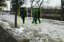
As we all know, false positive detections affect the precision of object detection, and the miss detection will affect the recall of object detection. Specially, we visualize the false positive detections and miss detection of the object detection results under AP50 in Fig. 8 and Fig. 9, respectively.


Appendix H Experiments On Bigger Models
Some bigger models, such as DeformableDETR (ResNet50, 39.8 parameters), achieve 44.50 mAP on COCO. In comparison, FemtoDet (72.7k parameters) only achieves 12.30 mAP on COCO due to differences in settings. FemtoDet is trained and tested on COCO with an input size of 416416, while DeformableDETR is trained and tested on COCO with an input size of 8001333. To address this issue, we compared FemtoDet and DeformableDETR (ResNet50) on PASCAL VOC under the same conditions. FemtoDet (8.3W on 3090Ti) achieved 46.3 AP50 / 22.0 mAP, while DeformableDETR (ResNet50, 134.0W on 3090Ti) achieved 70.7 AP50 / 26.8 mAP when tested on 416416 inputs. We also applied the proposed IBE to other larger models and observed consistent improvement in performance. For instance, MBV2 1.0 without IBE obtained 71.9 top1 Acc, while with IBE it achieved 72.2 top1 Acc on ImageNet. Similarly, yolox nano (MBV2 1.0 as backbone) without IBE achieved 53.1 mAP, while with IBE it achieved 53.5 mAP on VOC. These results demonstrate that FemtoDet achieves a reasonable tradeoff, and the IBE module consistently improves performance in larger models.
Appendix I Why not use ”R RS HO R+HO A” metric to present the results on TJU-DHD?
The missing rate (”R RS HO R+HO A”) used on TJU-DHD mainly focuses on challenging examples, such as small objects (RS) and heavy occlusion objects (HO). However, FemtoDet is better suited for detecting more accessible objects rather than these difficult examples. Therefore, we have presented AP-related results in Table 6 of the regular paper.
References
- [1] Abien Fred Agarap. Deep learning using rectified linear units (relu). arXiv preprint arXiv:1803.08375, 2018.
- [2] Yash Bhalgat, Jinwon Lee, Markus Nagel, Tijmen Blankevoort, and Nojun Kwak. Lsq+: Improving low-bit quantization through learnable offsets and better initialization. In Proceedings of the IEEE/CVF Conference on Computer Vision and Pattern Recognition Workshops, pages 696–697, 2020.
- [3] Abhiroop Bhattacharjee, Yeshwanth Venkatesha, Abhishek Moitra, and Priyadarshini Panda. Mime: Adapting a single neural network for multi-task inference with memory-efficient dynamic pruning. arXiv preprint arXiv:2204.05274, 2022.
- [4] Alexey Bochkovskiy, Chien-Yao Wang, and Hong-Yuan Mark Liao. Yolov4: Optimal speed and accuracy of object detection. arXiv preprint arXiv:2004.10934, 2020.
- [5] Yuxuan Cai, Hongjia Li, Geng Yuan, Wei Niu, Yanyu Li, Xulong Tang, Bin Ren, and Yanzhi Wang. Yolobile: Real-time object detection on mobile devices via compression-compilation co-design. In Proceedings of the AAAI Conference on Artificial Intelligence, volume 35, pages 955–963, 2021.
- [6] Peng Ding, Huaming Qian, and Shuai Chu. Slimyolov4: lightweight object detector based on yolov4. Journal of Real-Time Image Processing, pages 1–12, 2022.
- [7] Xiaohan Ding, Yuchen Guo, Guiguang Ding, and Jungong Han. Acnet: Strengthening the kernel skeletons for powerful cnn via asymmetric convolution blocks. In Proceedings of the IEEE/CVF international conference on computer vision, pages 1911–1920, 2019.
- [8] Xiaohan Ding, Xiangyu Zhang, Jungong Han, and Guiguang Ding. Scaling up your kernels to 31x31: Revisiting large kernel design in cnns. In Proceedings of the IEEE/CVF Conference on Computer Vision and Pattern Recognition, pages 11963–11975, 2022.
- [9] Stefan Elfwing, Eiji Uchibe, and Kenji Doya. Sigmoid-weighted linear units for neural network function approximation in reinforcement learning. Neural Networks, 107:3–11, 2018.
- [10] Zheng Ge, Songtao Liu, Feng Wang, Zeming Li, and Jian Sun. Yolox: Exceeding yolo series in 2021. arXiv preprint arXiv:2107.08430, 2021.
- [11] Golnaz Ghiasi, Tsung-Yi Lin, and Quoc V Le. Nas-fpn: Learning scalable feature pyramid architecture for object detection. In Proceedings of the IEEE/CVF conference on computer vision and pattern recognition, pages 7036–7045, 2019.
- [12] Raphael Gontijo-Lopes, Sylvia Smullin, Ekin Dogus Cubuk, and Ethan Dyer. Tradeoffs in data augmentation: An empirical study. In International Conference on Learning Representations, 2020.
- [13] Zichao Guo, Xiangyu Zhang, Haoyuan Mu, Wen Heng, Zechun Liu, Yichen Wei, and Jian Sun. Single path one-shot neural architecture search with uniform sampling. In European conference on computer vision, pages 544–560. Springer, 2020.
- [14] Hai Victor Habi, Roy H Jennings, and Arnon Netzer. Hmq: Hardware friendly mixed precision quantization block for cnns. In European Conference on Computer Vision, pages 448–463. Springer, 2020.
- [15] Kaiming He, Georgia Gkioxari, Piotr Dollár, and Ross Girshick. Mask r-cnn. In Proceedings of the IEEE international conference on computer vision, pages 2961–2969, 2017.
- [16] Kaiming He, Xiangyu Zhang, Shaoqing Ren, and Jian Sun. Deep residual learning for image recognition. In Proceedings of the IEEE conference on computer vision and pattern recognition, pages 770–778, 2016.
- [17] Dan Hendrycks and Kevin Gimpel. Gaussian error linear units (gelus). arXiv preprint arXiv:1606.08415, 2016.
- [18] Andrew G Howard, Menglong Zhu, Bo Chen, Dmitry Kalenichenko, Weijun Wang, Tobias Weyand, Marco Andreetto, and Hartwig Adam. Mobilenets: Efficient convolutional neural networks for mobile vision applications. arXiv preprint arXiv:1704.04861, 2017.
- [19] Alex Krizhevsky, Ilya Sutskever, and Geoffrey E Hinton. Imagenet classification with deep convolutional neural networks. Advances in neural information processing systems, 25, 2012.
- [20] Hei Law and Jia Deng. Cornernet: Detecting objects as paired keypoints. In Proceedings of the European conference on computer vision (ECCV), pages 734–750, 2018.
- [21] Xiang Li, Wenhai Wang, Lijun Wu, Shuo Chen, Xiaolin Hu, Jun Li, Jinhui Tang, and Jian Yang. Generalized focal loss: Learning qualified and distributed bounding boxes for dense object detection. Advances in Neural Information Processing Systems, 33:21002–21012, 2020.
- [22] Tsung-Yi Lin, Piotr Dollár, Ross Girshick, Kaiming He, Bharath Hariharan, and Serge Belongie. Feature pyramid networks for object detection. In Proceedings of the IEEE conference on computer vision and pattern recognition, pages 2117–2125, 2017.
- [23] Shu Liu, Lu Qi, Haifang Qin, Jianping Shi, and Jiaya Jia. Path aggregation network for instance segmentation. In Proceedings of the IEEE conference on computer vision and pattern recognition, pages 8759–8768, 2018.
- [24] Wei Liu, Dragomir Anguelov, Dumitru Erhan, Christian Szegedy, Scott Reed, Cheng-Yang Fu, and Alexander C Berg. Ssd: Single shot multibox detector. In European conference on computer vision, pages 21–37. Springer, 2016.
- [25] Ze Liu, Yutong Lin, Yue Cao, Han Hu, Yixuan Wei, Zheng Zhang, Stephen Lin, and Baining Guo. Swin transformer: Hierarchical vision transformer using shifted windows. In Proceedings of the IEEE/CVF International Conference on Computer Vision, pages 10012–10022, 2021.
- [26] Zhuang Liu, Hanzi Mao, Chao-Yuan Wu, Christoph Feichtenhofer, Trevor Darrell, and Saining Xie. A convnet for the 2020s. In Proceedings of the IEEE/CVF Conference on Computer Vision and Pattern Recognition, pages 11976–11986, 2022.
- [27] Ningning Ma, Xiangyu Zhang, Hai-Tao Zheng, and Jian Sun. Shufflenet v2: Practical guidelines for efficient cnn architecture design. In Proceedings of the European conference on computer vision (ECCV), pages 116–131, 2018.
- [28] Yanwei Pang, Jiale Cao, Yazhao Li, Jin Xie, Hanqing Sun, and Jinfeng Gong. Tju-dhd: A diverse high-resolution dataset for object detection. IEEE Transactions on Image Processing, 30:207–219, 2020.
- [29] RangiLyu. Nanodet-plus: Super fast and high accuracy lightweight anchor-free object detection model. https://github.com/RangiLyu/nanodet, 2021.
- [30] Joseph Redmon, Santosh Divvala, Ross Girshick, and Ali Farhadi. You only look once: Unified, real-time object detection. In Proceedings of the IEEE conference on computer vision and pattern recognition, pages 779–788, 2016.
- [31] Joseph Redmon and Ali Farhadi. Yolo9000: better, faster, stronger. In Proceedings of the IEEE conference on computer vision and pattern recognition, pages 7263–7271, 2017.
- [32] Joseph Redmon and Ali Farhadi. Yolov3: An incremental improvement. arXiv preprint arXiv:1804.02767, 2018.
- [33] Shaoqing Ren, Kaiming He, Ross Girshick, and Jian Sun. Faster r-cnn: Towards real-time object detection with region proposal networks. Advances in neural information processing systems, 28, 2015.
- [34] Mark Sandler, Andrew Howard, Menglong Zhu, Andrey Zhmoginov, and Liang-Chieh Chen. Mobilenetv2: Inverted residuals and linear bottlenecks. In Proceedings of the IEEE conference on computer vision and pattern recognition, pages 4510–4520, 2018.
- [35] Mohammad Javad Shafiee, Brendan Chywl, Francis Li, and Alexander Wong. Fast yolo: A fast you only look once system for real-time embedded object detection in video. arXiv preprint arXiv:1709.05943, 2017.
- [36] Zhuo Su, Wenzhe Liu, Zitong Yu, Dewen Hu, Qing Liao, Qi Tian, Matti Pietikäinen, and Li Liu. Pixel difference networks for efficient edge detection. In Proceedings of the IEEE/CVF International Conference on Computer Vision, pages 5117–5127, 2021.
- [37] Peize Sun, Rufeng Zhang, Yi Jiang, Tao Kong, Chenfeng Xu, Wei Zhan, Masayoshi Tomizuka, Lei Li, Zehuan Yuan, Changhu Wang, et al. Sparse r-cnn: End-to-end object detection with learnable proposals. In Proceedings of the IEEE/CVF conference on computer vision and pattern recognition, pages 14454–14463, 2021.
- [38] Mingxing Tan, Ruoming Pang, and Quoc V Le. Efficientdet: Scalable and efficient object detection. In Proceedings of the IEEE/CVF conference on computer vision and pattern recognition, pages 10781–10790, 2020.
- [39] Zhi Tian, Chunhua Shen, Hao Chen, and Tong He. Fcos: Fully convolutional one-stage object detection. In Proceedings of the IEEE/CVF international conference on computer vision, pages 9627–9636, 2019.
- [40] Vincent Torre and Tomaso A Poggio. On edge detection. IEEE Transactions on Pattern Analysis and Machine Intelligence, (2):147–163, 1986.
- [41] Jin Xie, Yanwei Pang, Jing Nie, Jiale Cao, and Jungong Han. Latent feature pyramid network for object detection. IEEE Transactions on Multimedia, 2022.
- [42] Jin Xu, Xu Tan, Kaitao Song, Renqian Luo, Yichong Leng, Tao Qin, Tie-Yan Liu, and Jian Li. Analyzing and mitigating interference in neural architecture search. In International Conference on Machine Learning, pages 24646–24662. PMLR, 2022.
- [43] Shangliang Xu, Xinxin Wang, Wenyu Lv, Qinyao Chang, Cheng Cui, Kaipeng Deng, Guanzhong Wang, Qingqing Dang, Shengyu Wei, Yuning Du, et al. Pp-yoloe: An evolved version of yolo. arXiv preprint arXiv:2203.16250, 2022.
- [44] Haichuan Yang, Yuhao Zhu, and Ji Liu. Ecc: Platform-independent energy-constrained deep neural network compression via a bilinear regression model. In Proceedings of the IEEE/CVF Conference on Computer Vision and Pattern Recognition, pages 11206–11215, 2019.
- [45] Xinyi Ying, Yingqian Wang, Longguang Wang, Weidong Sheng, Li Liu, Zaipin Lin, and Shilin Zho. Mocopnet: Exploring local motion and contrast priors for infrared small target super-resolution. arXiv preprint arXiv:2201.01014, 2022.
- [46] Guanghua Yu, Qinyao Chang, Wenyu Lv, Chang Xu, Cheng Cui, Wei Ji, Qingqing Dang, Kaipeng Deng, Guanzhong Wang, Yuning Du, et al. Pp-picodet: A better real-time object detector on mobile devices. arXiv preprint arXiv:2111.00902, 2021.
- [47] Jiahui Yu and Thomas Huang. Autoslim: Towards one-shot architecture search for channel numbers. arXiv preprint arXiv:1903.11728, 2019.
- [48] Hongyi Zhang, Moustapha Cisse, Yann N Dauphin, and David Lopez-Paz. mixup: Beyond empirical risk minimization. arXiv preprint arXiv:1710.09412, 2017.
- [49] Haibo Zhang, Shulin Zhao, Ashutosh Pattnaik, Mahmut T Kandemir, Anand Sivasubramaniam, and Chita R Das. Distilling the essence of raw video to reduce memory usage and energy at edge devices. In Proceedings of the 52nd Annual IEEE/ACM international symposium on microarchitecture, pages 657–669, 2019.
- [50] Shifeng Zhang, Cheng Chi, Yongqiang Yao, Zhen Lei, and Stan Z Li. Bridging the gap between anchor-based and anchor-free detection via adaptive training sample selection. In Proceedings of the IEEE/CVF conference on computer vision and pattern recognition, pages 9759–9768, 2020.
- [51] Djemel Ziou, Salvatore Tabbone, et al. Edge detection techniques-an overview. Pattern Recognition and Image Analysis C/C of Raspoznavaniye Obrazov I Analiz Izobrazhenii, 8:537–559, 1998.