Feedback voltage driven chaos in a three-terminal spin-torque oscillator

Figures 2(a)-2(c) summarize typical dynamics of $m_{x}$ (red) and $m_{y}$ (blue) near $t=0$, where $\nu$ is (a) $0$, (b) $0.1$, and (c) $0.5$, while the Fourier spectra, $|m_{x}(f)|$, of $m_{x}(t)$ for these $\nu$ are shown in Figs. 2(d)-2(f). The Fourier spectra for various $\nu$ are summarized in Fig. 3. In the absence of the feedback effect ($\nu=0$), an auto-oscillation with a single main frequency is excited, as in the case of the conventional three-terminal STOs [51]; see Figs. 2(a) and 2(d), as well as the inset in Fig. 2(a). In the presence of the feedback effect, however, the dynamics is largely modulated, although the dynamics during a short time scale looks similar to a simple auto-oscillation; see Fig. 2(b) and compare the insets in Fig. 2(a) and 2(b). The complexity of the dynamics is also found from the Fourier spectrum in Fig. 2(e), where the spectra shows broadened structure. The magnetization switching is also observed for different values of $\nu$, as shown in Fig. 2(c). Note that the oscillation amplitude repeats the cycles of amplification and reduction before the switching, which is also reflected in the broadened structure of the Fourier spectrum in Fig. 2(f). This switching behavior is quite different from the conventional spin-transfer (spin-orbit) torque switching [52, 45], where the work done by the spin-transfer torque monotonically supplies energy into the ferromagnet and thus, the oscillation amplitude increases monotonically. The complex behavior before the magnetization switching found in Fig. 2(c) suggests that the dynamics is classified as transient chaos [38], where the nonlinear dynamical system shows chaotic behavior before saturating to a fixed point.

Summarizing the results, it is shown that the feedback VCMA effect causes the modulation of the oscillation amplitude in the STO, and the dynamics becomes complex. The complexity of the dynamics results in the broadened structure of the Fourier spectra, as summarized in Fig. 3. These results are similar to the characteristics found in chaotic spintronics devices with feedback current or magnetic field [16, 18, 19]. We should, however, recall that an appearance of complex dynamics is not a direct evidence of the existence of chaos. Although the complexity of dynamics is a typical characteristic of chaos, not all complex dynamics is classified as chaos. One way to identify chaos is to evaluate the Lyapunov exponent [1].

The Lyapunov exponent is an instantaneous expansion rate of a distance between two solutions of the LLG equation having infinitesimally different initial conditions. The expansion rate is usually time and/or position dependent, and thus, a statistical average of temporal Lyapunov exponent is often evaluated [53, 54, 55, 56, 57]. The Lyapunov exponent in spintronics system has been studied previously [8, 9, 17, 46, 47, 48]. However, a different method is necessary for evaluating the Lyapunov exponent in the feedback system because not only the expansion rate of the magnetization at the present time but also that in the past time should be evaluated. Therefore, let us first explain the evaluation method of the Lyapunov exponent in the present system.

Let us denote the solution of the LLG equation with an initial condition $\mathbf{m}(t)$. Note that we need to store the value of $N+1$ $\mathbf{m}$ [$\mathbf{m}(t-\tau)$, $\mathbf{m}(t-\tau+\Delta t)$, $\mathbf{m}(t-\tau+2\Delta t)$, $\cdots$, $\mathbf{m}(t-\Delta t)$, $\mathbf{m}(t)$] for performing the numerical simulation, where $\mathbf{m}(t-\tau),\cdots,\mathbf{m}(t-\Delta t)$ are the past values of $\mathbf{m}(t)$ and are used as feedback signal. Assuming that we start to evaluate the Lyapunov exponent from a certain time $t=t_{\rm init}$, let us denote the set of these vectors as

$$\mathbf{Y}(t_{\rm init})=\begin{pmatrix}\mathbf{m}(t_{\rm init}-\tau)\\ \mathbf{m}(t_{\rm init}-\tau+\Delta t)\\ \vdots\\ \mathbf{m}(t_{\rm init})\end{pmatrix}.$$

(3)

Their values are determined by the LLG equation with the initial condition mentioned in Sec. II. These vectors are the dynamical variables in the feedback system [22]. Since each vector $\mathbf{m}$ is a three-dimensional vector with a constraint $|\mathbf{m}|=1$, the number of the dynamical degree of freedom is $2(N+1)$, as mentioned earlier. We note that the ordering of these $N+1$ $\mathbf{m}$ does not affect the evaluation of the distance in the phase space, as well as the Lyapunov exponent, by the method mentioned below and thus, is arbitrary. To evaluate the Lyapunov exponent, for each $\mathbf{m}[t_{\rm init}-(N-k)\Delta t]$ ($k=0,1,\cdots,N$), we introduce the zenith and azimuth angles in a spherical coordinate, $\theta_{k}=\cos^{-1}m_{z}[t_{\rm init}-(N-k)\Delta t]$ and $\varphi_{k}=\tan^{-1}\{m_{y}[t_{\rm init}-(N-k)\Delta t]/m_{x}[t_{\rm init}-(N-k)\Delta t]\}$. Then, we introduce $N+1$ $\mathbf{m}_{1}$, whose zenith and azimuth angles, $\theta_{1,k}=\cos^{-1}m_{1,k,z}[t_{\rm init}-(N-k)\Delta t]$ and $\varphi_{1,k}=\tan^{-1}\{m_{1,k,y}[t_{\rm init}-(N-k)\Delta t]/m_{1,k,x}[t_{\rm init}-(N-k)\Delta t]\}$, are defined by shifting $\theta_{k}$ and $\varphi_{k}$ with infinitesimal differences ($|\epsilon_{1,k,\theta}|,|\epsilon_{1,k,\varphi}|\ll 1$) as $\theta_{1,k}=\theta_{k}+\epsilon_{1,k,\theta}$ and $\varphi_{1,k}=\varphi_{k}+\epsilon_{1,k,\varphi}$. Here, the subscript “1” is applied to the variables necessary to evaluate the first temporal Lyapunov exponent defined below. The distance between $\mathbf{m}[t_{\rm init}-(N-k)\Delta t]$ and $\mathbf{m}_{1}[t_{\rm init}-(N-k)\Delta t]$ at time $t_{\rm init}$ is given by $\epsilon_{1,k}=\sqrt{\epsilon_{1,k,\theta}^{2}+\epsilon_{1,k,\varphi}^{2}}$, and their sum is $\epsilon=\sum_{k=0}^{N}\epsilon_{1,k}$. Also, we introduce

$$\mathbf{Y}_{1}(t_{\rm init})=\begin{pmatrix}\mathbf{m}_{1}(t_{\rm init}-\tau)\\ \mathbf{m}_{1}(t_{\rm init}-\tau+\Delta t)\\ \vdots\\ \mathbf{m}_{1}(t_{\rm init})\end{pmatrix}.$$

(4)

Therefore, $\epsilon$ can be regarded as a distance between $\mathbf{Y}(t_{\rm init})$ and $\mathbf{Y}_{1}(t_{\rm init})$. Then, we evaluate the time evolution of $\mathbf{m}(t_{\rm init})$ and $\mathbf{m}_{1}(t_{\rm init})$ from time $t_{\rm init}$ to $t_{\rm init}+\Delta t$ by solving the LLG equation and obtain $\mathbf{m}(t_{\rm init}+\Delta t)$ and $\mathbf{m}_{1}(t_{\rm init}+\Delta t)$. Recall that the values of $\mathbf{m}(t_{\rm init}-\tau)$ and $\mathbf{m}_{1}(t_{\rm init}-\tau)$ in $\mathbf{Y}(t_{\rm init})$ and $\mathbf{Y}_{1}(t_{\rm init})$, respectively, are used as the feedback term to evaluate the time evolution and become no longer necessary to be stored. Thus, we update $\mathbf{Y}$ and $\mathbf{Y}_{1}$ by replacing $\mathbf{m}(t_{\rm init}-\tau)$ and $\mathbf{m}_{1}(t_{\rm init}-\tau)$ in them respectively with $\mathbf{m}(t_{\rm init}+\Delta t)$ and $\mathbf{m}_{1}(t_{\rm init}+\Delta t)$ as

$$\mathbf{Y}(t_{\rm init}+\Delta t)=\begin{pmatrix}\mathbf{m}(t_{\rm init}+\Delta t)\\ \mathbf{m}(t_{\rm init}-\tau+\Delta t)\\ \vdots\\ \mathbf{m}(t_{\rm init})\end{pmatrix},$$

(5)

$$\mathbf{Y}_{1}(t_{\rm init}+\Delta t)=\begin{pmatrix}\mathbf{m}_{1}(t_{\rm init}+\Delta t)\\ \mathbf{m}_{1}(t_{\rm init}-\tau+\Delta t)\\ \vdots\\ \mathbf{m}_{1}(t_{\rm init})\end{pmatrix}.$$

(6)

Note that the distance $\epsilon_{1}$ between $\mathbf{Y}(t_{\rm init}+\Delta t)$ and $\mathbf{Y}_{1}(t_{\rm init}+\Delta t)$ is different from that ($\epsilon$) between $\mathbf{Y}(t_{\rm init})$ and $\mathbf{Y}_{1}(t_{\rm init})$. They are related as $\epsilon_{1}=\epsilon-\epsilon_{1,0}+\epsilon_{1,0}^{\prime}$, where $\epsilon_{1,0}^{\prime}$ is the distance between $\mathbf{m}(t_{\rm init}+\Delta t)$ and $\mathbf{m}_{1}(t_{\rm init}+\Delta t)$, in terms of $\theta_{0}^{\prime}=\cos^{-1}m_{z}(t_{\rm init}+\Delta t)$, $\varphi_{0}^{\prime}=\tan^{-1}[m_{y}(t_{\rm init}+\Delta t)/m_{x}(t_{\rm init}+\Delta t)]$, $\theta_{1,0}^{\prime}=\cos^{-1}m_{1,z}(t_{\rm init}+\Delta t)$, and $\varphi_{1,0}^{\prime}=\tan^{-1}[m_{1,y}(t_{\rm init}+\Delta t)/m_{1,x}(t_{\rm init}+\Delta t)]$. The expansion rate of the solution of the LLG equation during $[t_{\rm init},t_{\rm init}+\Delta t]$ is given by $\epsilon_{1}/\epsilon$. Therefore, a temporal Lyapunov exponent at time $t_{\rm init}+\Delta t$ is defined as

$$\lambda_{1}=\frac{1}{\Delta t}\ln\frac{\epsilon_{1}}{\epsilon}.$$

(7)

We repeat this procedure and evaluate the temporal Lyapunov exponent every time (in this work, we choose $t_{\rm init}=\tau$), i.e., we start to evaluate the temporal Lyapunov exponent from $t=\tau$). In general, at time $t_{n}=t_{\rm init}+(n-1)\Delta t$ ($n=1,2,\cdots$), we introduce $\mathbf{Y}_{n}(t_{n})$, which consists of $N+1$ $\mathbf{m}$, $\mathbf{m}_{n}(t_{n}-\tau)$, $\mathbf{m}_{n}(t_{n}-\tau+\Delta t)$, $\cdots$, $\mathbf{m}_{n}(t_{n})$, and differs from $\mathbf{Y}(t_{n})$ with a distance $\epsilon$, i.e., $|\mathbf{Y}(t_{n})-\mathbf{Y}_{n}(t_{n})|=\epsilon$. Here, $\mathbf{m}_{n}(t_{n}-\tau+k\Delta t)$ is defined from $\mathbf{m}(t_{n}-\tau+k\Delta t)$ so that the direction from $\mathbf{m}(t_{n}-\tau+k\Delta t)$ to $\mathbf{m}_{n}(t_{n}-\tau+k\Delta t)$ is the most expanded direction; see Refs. [16, 48, 53]. Then, the time evolution of $\mathbf{m}(t_{n})$ and $\mathbf{m}_{n}(t_{n})$ to $\mathbf{m}(t_{n}+\Delta t)$ and $\mathbf{m}_{n}(t_{n}+\Delta t)$ are evaluated, and $\mathbf{Y}(t_{n})$ and $\mathbf{Y}_{n}(t_{n})$ are updated to $\mathbf{Y}(t_{n}+\Delta t)$ and $\mathbf{Y}_{n}(t_{n}+\Delta t)$, respectively, by replacing $\mathbf{m}(t_{n}-\tau)$ and $\mathbf{m}_{n}(t_{n}-\tau)$ in them with $\mathbf{m}(t_{n}+\Delta t)$ and $\mathbf{m}_{n}(t_{n}+\Delta t)$. From their distance $\epsilon_{n}=|\mathbf{Y}_{n}(t_{n}+\Delta t)-\mathbf{Y}(t_{n}+\Delta t)|$, the $n$th temporal Lyapunov exponent is defined as $\lambda_{n}=(1/\Delta t)\ln(\epsilon_{n}/\epsilon)$. After that, we introduce $\mathbf{Y}_{n+1}(t_{n}+\Delta t)$ from $\mathbf{Y}(t_{n}+\Delta t)$, where the elements in $\mathbf{Y}_{n+1}(t_{n}+\Delta t)$ are determined by moving those in $\mathbf{Y}(t_{n}+\Delta t)$ to the most expanded direction with the condition $|\mathbf{Y}(t_{n}+\Delta t)-\mathbf{Y}_{n+1}(t_{n}+\Delta t)|=\epsilon$, as we define $\mathbf{Y}_{n}(t_{n})$ mentioned above. Note that the most expanded direction is determined by $\mathbf{Y}(t_{n}+\Delta t)$ and $\mathbf{Y}_{n}(t_{n}+\Delta t)$; see Refs. [16, 48, 53] in detail. Finally, the Lyapunov exponent $\varLambda$ is defined as a statistical average of the temporal Lyapunov exponents as $\varLambda=(1/\mathscr{N})\sum_{n=1}^{\mathscr{N}}\lambda_{n}$ [16], where $\mathscr{N}$ is the number of the averaging and $\lambda_{n}$ is the $n$th temporal Lyapunov exponent (since we prepare $\mathbf{m}_{1}$ at $t=\tau$, as mentioned above, and the time increment $\Delta t=1$ ps while $t_{\rm max}=1$ $\mu$s, $\mathscr{N}=979999$ in this work).

The sign of the Lyapunov exponent indicates the dynamical state of the system, i.e., negative exponent corresponds to dynamics saturating to a fixed point, zero exponent corresponds to a periodic dynamics, and positive exponent corresponds to chaos. Figure 4 summarizes the Lyapunov exponent for various $\nu$’s. The value is zero at $\nu=0$, i.e., in the absence of the feedback effect, because the magnetization dynamics in this case is a periodic oscillation (auto-oscillation), as shown in Fig. 2(a). For finite feedback effect ($\nu\neq 0$), such as the dynamics in Fig. 2(b), the Lyapunov exponent becomes positive, which can be an evidence of the existence of chaos in the present system. The Lyapunov exponent can also be negative for some $\nu$’s when the magnetization switches its direction, as shown in Fig. 2(c). Summarizing them, the sign of the Lyapunov exponent reasonably reflects the dynamical behavior of the magnetization.

Note that analyses on both temporal dynamics in Fig. 2 and statistical property (Lyapunov exponent) in Fig. 4 are necessary to identify dynamical state of the magnetization. The temporal analysis clarifies the existence of complex dynamics, at least as temporary, which may be failed to notice from just evaluating the Lyapunov exponent. For example, for the dynamics shown in Fig. 2(c), chaotic behavior that appeared initially might be overlooked when only the Lyapunov exponent is evaluated. On the other hand, the evaluation of the Lyapunov exponent can be used as a figure of merit to distinguish between chaos and complex but non-chaotic dynamics, which is hard to determine from just observing temporal dynamics. While the temporal dynamics in STOs has been frequently measured and used in practical applications, one may be interested in how to estimate the Lyapunov exponent experimentally. In experiments, it is difficult to control the initial state of the magnetization, and thus, the evaluation method of the Lyapunov exponent used in the numerical simulation is hardly applicable. There are, however, various methods to estimate the Lyapunov exponent from experimental data by reproducing the dynamical trajectory in an embedded space [20] or identify chaos from different quantities, such as noise limit [58, 59, 11, 18]. Therefore, it will be possible to examine the validity of the present results by experiments in the future.

Recall that the identification of chaos sometimes depends on the measurement time $t_{\rm max}$, especially when transient chaos possibly occurs [38]. For example, we did not observe magnetization switching until $t_{\rm max}=1$ $\mu$s for $\nu=0.1$ shown in Fig. 2(b); therefore, the corresponding Lyapunov exponent for this $\nu$ is positive, as shown in Fig. 4. If we use, however, $t_{\rm max}$ longer than $1$ $\mu$s, a switching may occur; in this case, the Lyapunov exponent will be negative and the dynamics will be classified as transient chaos. On the other hand, if we, for example, use $t_{\rm max}=100$ ns, the dynamics for $\nu=0.5$ shown in Fig. 2(c) may be classified as chaos and the Lyapunov exponent becomes positive because at $t=100$ ns, there is no switching. As shown in these examples, the identification of chaos depends on the measurement time. This is not a particular property for spintronics devices; rather, this is a general consequence in chaotic system [38]. It is generally difficult to estimate the transient time, if transient chaos exists, because it depends not only on the values of parameters but also on the initial conditions, etc [38]. The time scale during which chaos can be kept determines the manipulation time of chaos applications, and thus, is of great interest. We keep this issue as a future work.

For a while, let us neglect the feedback effect in the demagnetization field, for simplicity. The previous works clarified that there are two characteristic current densities for the auto-oscillation of the magnetization in an in-plane magnetized ferromagnet. One is a critical current density $J_{\rm c}$ given by [52, 45, 60, 61, 62],

$$J_{\rm c}=\frac{2\alpha eMd}{\hbar\vartheta}\left(H_{\rm K}+2\pi M\right),$$

(8)

while the other is a threshold current density $J^{*}$ given by [63, 64, 65, 66],

$$J^{*}=\frac{4\alpha eMd}{\pi\hbar\vartheta}\sqrt{4\pi M\left(H_{\rm K}+4\pi M\right)}.$$

(9)

These current densities relate to the stability of the magnetization having a magnetic potential energy density $E$, which relates to the magnetic field $\mathbf{H}$ via $\mathbf{H}=-\partial E/\partial(M\mathbf{m})$ and is given by

$$E=-\frac{MH_{\rm K}}{2}m_{y}^{2}+2\pi M^{2}m_{z}^{2}.$$

(10)

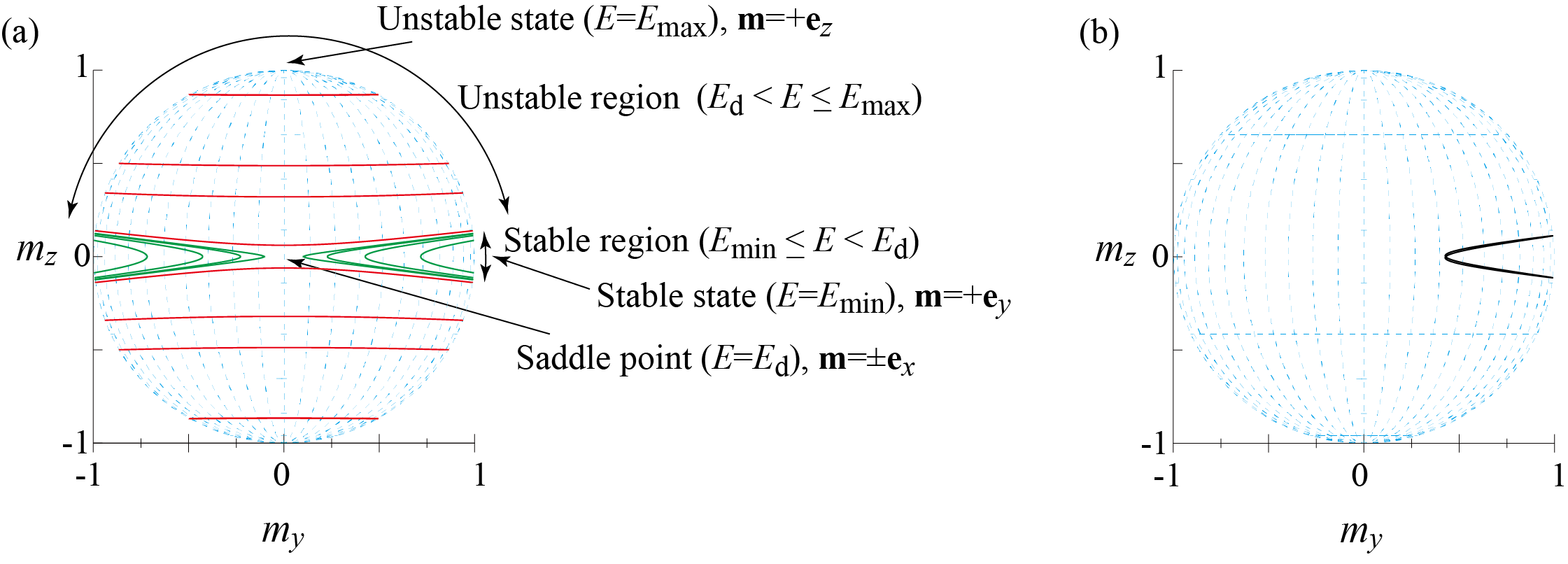
The energy density $E$ has two minima ($E_{\rm min}=-MH_{\rm K}/2$) at $\mathbf{m}=\pm\mathbf{e}_{y}$, two saddle points ($E_{\rm d}=0$) at $\mathbf{m}=\pm\mathbf{e}_{x}$, and two maxima ($E_{\rm max}=2\pi M^{2}$) at $\mathbf{m}=\pm\mathbf{e}_{z}$. Recall that a constant energy curve of $E$ is identical to a solution of Landau-Lifshitz (LL) equation, $d\mathbf{m}/dt=-\gamma\mathbf{m}\times\mathbf{H}$, which is the LLG equation without spin-transfer and damping torques. In Fig. 5(a), we show examples of constant energy lines. Since the LLG equation conserves the magnitude of the magnetization ($|\mathbf{m}|=1$), the constant energy lines can be represented as lines on a unit sphere. Let us call the region satisfying $E_{\rm min}\leq E<E_{\rm d}$ ($E_{\rm d}<E\leq E_{\rm max}$) stable (unstable) region. In particular, the points $\mathbf{m}=\pm\mathbf{e}_{y}(\pm\mathbf{e}_{z}$) are called stable (unstable) states. Note that the constant energy lines in the stable region are densely distributed due to the large demagnetization field. It should be noted that the trajectory of the conventional auto-oscillation state is well approximated by a constant energy line. This is because the existence of a sustainable oscillation means that the spin-transfer (spin-orbit) and damping torques balance each other and thus, $E$ is approximately kept to be constant; see also Appendix A. For example, in Fig. 5(b), we show the steady-state dynamics in Fig. 2(a) as a trajectory, which is similar to a constant energy line in Fig. 5(a). Note also that this oscillation trajectory stays inside the stable region in Fig. 5(a), which means that the energy in an auto-oscillation state is in the range of $E_{\rm min}<E<E_{\rm d}$.

The critical current density $J_{\rm c}$ is derived from the LLG equation linearized near the stable state and determines the stability around it; see also Appendix A. On the other hand, the threshold current density $J^{*}$ is derived from the stability condition of the LLG equation averaged over a constant energy line including the saddle points [65]; see also Appendix A. The auto-oscillation of the magnetization occurs when the current density $J$ is in the range of $J_{\rm c}<J<J^{*}$ (see also Appendix A), whereas the magnetization switching occurs when $J>J^{*}$. In the present system, the values of $J_{\rm c}$ and $J^{*}$ in the absence of the feedback effect are $13.1$ MA/cm² and $16.3$ MA/cm², respectively. Recall that the current density $J$ was $15.0$ MA/cm², as shown in Table 1. Therefore, the condition $J_{\rm c}<J<J^{*}$ is satisfied, and the auto-oscillation was observed, which is shown in Fig. 2(a).

Now let us consider the role of the feedback effect. Recall that the feedback effect modulates the demagnetization field as $4\pi M\to 4\pi M\{1+\nu[m_{x}(t-\tau)]^{2}\}$. As mentioned in Sec. II, we focused on the positive $\nu$ case. This is because we intend to excite chaos by the feedback effect. For this purpose, the magnetization should show a sustainable dynamics, such as an auto-oscillation, while dynamics saturating to a fixed point, such as a magnetization switching, should be avoided. In our case, when $\nu$ is positive, the modulation of the demagnetization field by the feedback VCMA effect enhances the demagnetization field. Therefore, the threshold current density increases compared with that without the feedback effect, which makes the magnetization switching more difficult to happen. On the other hand, if $\nu$ is negative, the threshold current density becomes small, and the magnetization switching will be easier to appear. Therefore, expectation was that to use positive $\nu$ is suitable for exciting chaos in the present system. However, the numerical simulations show that, even though we choose the positive $\nu$, the magnetization switching occasionally occurs, as shown in Fig. 2(c). This is the reason why we consider that the appearance of the transient chaos (magnetization switching) is non-trivial.

To clarify the origin of the magnetization switching, it is helpful to compare this switching to the conventional auto-oscillation. As mentioned in Sec. IV.1, the trajectory of the conventional auto-oscillation stays inside the stable region, and thus, the energy density $E$ satisfies $E<E_{\rm d}$. Accordingly, the appearance of the magnetization switching in the presence of the feedback effect indicates that the magnetization crosses a constant energy line including the saddle point, even though the current density $J$ is smaller than the threshold current density. To confirm it, we introduce a normalized (dimensionless) energy density $\varepsilon$ defined as

$$\varepsilon=-\frac{k}{2}m_{y}^{2}+\frac{1+\nu[m_{x}(t-\tau)]^{2}}{2}m_{z}^{2},$$

(11)

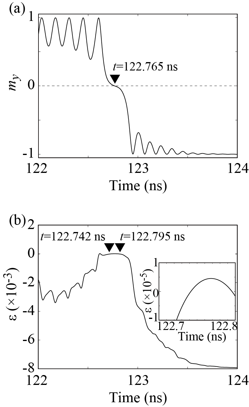
where $k=H_{\rm K}/(4\pi M)$. We note that Eq. (11) relates to Eq. (10) via $E=4\pi M^{2}\varepsilon$ with $\nu\to 0$. In Eq. (11), the feedback term $m_{x}(t-\tau)$ is treated as a time-dependent parameter. Then, the saddle points of $\varepsilon$ still locate at $\mathbf{m}=\pm\mathbf{e}_{x}$, and the corresponding saddle point energy is $\varepsilon_{\rm d}=0$. We notice that the magnetization switching in the transient chaos accompanies the change of $\varepsilon$ from $\varepsilon<\varepsilon_{\rm d}$ to $\varepsilon>\varepsilon_{\rm d}$. For example, Fig. 6(a) shows the time evolution of $m_{y}$ near the switching in Fig. 2(c), where $m_{y}$ changes from positive to negative at $t=122.765$ ns. The time evolution of $\varepsilon$ near the switching is shown in Fig. 6(b), where we confirm that $\varepsilon$ becomes positive in the range of $122.742\leq t\leq 122.795$ ns, i.e., $\varepsilon$ around the magnetization switching indeed becomes larger than $\varepsilon_{\rm d}(=0)$ [see also the inset of Fig. 6(b)]. These results indicate that $\varepsilon$ is no longer kept to be constant and can be larger than the saddle-point energy density when the transient chaos occurs. The result is in contrast to the conventional auto-oscillation, where $E$ is approximately constant and is in the region of $E<E_{\rm d}$. We also note that the temporal change of the energy density $\varepsilon$ is different from the conventional spin-transfer torque switching without feedback effect, where an averaged amplitude, as well as energy density, of the magnetization oscillation increases monotonically due to the energy injection by the work done by the spin-transfer torque.

Now let us investigate how the magnetization crosses the constant energy line including the saddle point. Note that a constant energy line of $\varepsilon$ changes temporally due to the presence of the feedback term. In other words, the stable and unstable regions are narrowed or expanded temporally, according to the oscillation of the feedback term $[m_{x}(t-\tau)]^{2}$. We then notice that the switching occurs when the feedback term narrows the stable region. This can be confirmed from Fig. 7(a), where we show the constant energy lines including the saddle points at various times ($t=122.730$, $122.736$, and $122.742$ ns) just before the magnetization switching. At the same time, we also notice that the magnetization locates close to the saddle point and its precession direction points from the stable state ($\mathbf{m}\parallel\mathbf{e}_{y}$) to the saddle point ($\mathbf{m}\parallel\mathbf{e}_{x}$). This can be confirmed from Fig. 7(b), where we show the magnetization directions by dots and again show the constant energy lines including the saddle point by solid lines. The dotted arrows indicate the directions of their temporal changes. It is shown that the constant energy line and the magnetization move in the opposite directions. One may consider that the change of the constant energy line is small compared to that of the magnetization. Recall, however, that the stable regions are narrow due to the large demagnetization field and the constant energy lines inside the regions are densely distributed; thus, a small change of the constant energy line including the saddle point significantly affects the alignment of the other constant energy lines. As a result, the magnetization crosses the constant energy line including the saddle point. Hence, the magnetization enters the unstable region, precesses around the demagnetization field, and relaxes to the switched state.

Summarizing these results, we consider that the magnetization switching occurs when the following conditions are coincidentally satisfied. First, the magnetization should be located near the saddle point, or equivalently, far away from the easy axis. It occurs approximately periodically because the magnetization precesses around the easy axis. Second, the precession direction points to the saddle point, which also occurs almost periodically. Third, the modulation of the demagnetization field narrows the stable region. Recall that the stable region repeats narrowing and expanding because the feedback term $[m_{x}(t-\tau)]^{2}$ oscillates. In Fig. 7(c), we show a schematic illustration, which roughly summarizes a situation satisfying these conditions. We emphasize that these conditions should be satisfied simultaneously. For example, even if the modulation of the demagnetization field narrows the stable region and as a result, the magnetization is located at a point outside a constant energy line including the saddle point, the switching will not occur if the location is close to the stable state. This is because a relatively long time is necessary for switching in this case, however, before that, the stable region may expand according to the temporal change of the feedback term. Therefore, the magnetization switching rarely occurs and/or strongly depends on the values of the parameters and the initial condition. This leads to that, although chaos is excited over a wide range of the parameter $\nu$, transient chaos is also observed in some cases.

References

- Strogatz [2001] S. H. Strogatz, Nonlinear Dynamics and Chaos: With Applications to Physics, Biology, Chemistry, and Engineering, 1st ed. (Westview Press, Boulder, 2001).
- Stojanovski and Kocarev [2001] T. Stojanovski and L. Kocarev, Chaos-based random number generators-part I: analysis, IEEE Trans. Circuits Syst. I: Fundamental and Theory 48, 281 (2001).
- Cuomo and Oppenheim [1993] K. M. Cuomo and A. V. Oppenheim, Circuit Implementation of Synchornized Chaos, with Applications to Communications, Phys. Rev. Lett. 71, 65 (1993).
- Verstraeten et al. [2007] D. Verstraeten, B. Schrauwen, M. D’Haene, and D. Stroobandt, An experimental unification of reservoir computing methods, Neural Netw. 20, 391 (2007).
- Wigen [1994] P. H. Wigen, ed., Nonlinear Phenomena and Chaos in Magnetic Materials (World Scientific Publishing, Singapore, 1994).
- Mino and Wigen [2001] M. Mino and P. Wigen, Strange Attractor of Controlled Chaos in Yttrium Iron Garnet Films, J. Phys. Soc. Jpn. 70, 2161 (2001).
- Kudo et al. [2006] K. Kudo, R. Sato, and K. Mizushima, Synchronized Magnetization Oscillations in F/N/F Nanopillars, Jpn. J. Appl. Phys. 45, 3869 (2006).
- Li et al. [2006] Z. Li, Y. C. Li, and S. Zhang, Dynamic magnetization states of a spin valve in the presence of dc and ac currents: Synchronization, modification, and chaos, Phys. Rev. B 74, 054417 (2006).
- Yang et al. [2007] Z. Yang, S. Zhang, and Y. C. Li, Chaotic Dynamics of Spin-Valve Oscillators, Phys. Rev. Lett. 99, 134101 (2007).
- Petit-Watelot et al. [2012] S. Petit-Watelot, J.-V. Kim, A. Ruotolo, R. M. Otxoa, K. Bouzehouane, J. Grollier, A. Vansteenkiste, B. V. de Wiele, V. Cros, and T. Devolder, Commensurability and chaos in magnetic vortex oscillations, Nat. Phys. 8, 682 (2012).
- Devolder et al. [2019] T. Devolder, D. Rontani, S. Petit-Watelot, K. Bouzehouane, S. Andrieu, J. Letang, M.-W. Yoo, J.-P. Adam, C. Chappert, S. Girod, V. Cros, M. Sciamanna, and J.-V. Kim, Chaos in magnetic nanocontact vortex oscillators, Phys. Rev. Lett. 123, 147701 (2019).
- Bondarenko et al. [2019] A. V. Bondarenko, E. Holmgren, Z. W. Li, B. A. Ivanov, and V. Korenivski, Chaotic dynamics in spin-vortex pairs, Phys. Rev. B 99, 054402 (2019).
- Montoya et al. [2019] E. A. Montoya, S. Perna, Y.-J. Chen, J. A. Katine, M. d’Aquino, C. Serpico, and I. N. Krivorotov, Magnetization reversal driven by low dimensional chaos in a nanoscale ferromagnet, Nat. Commun. 10, 543 (2019).
- Taniguchi [2019] T. Taniguchi, Synchronized, periodic, and chaotic dynamics in spin torque oscillator with two free layers, J. Magn. Magn. Mater. 483, 281 (2019).
- Williame et al. [2019] J. Williame, A. D. Accoily, D. Rontani, M. Sciamanna, and J.-V. Kim, Chaotic dynamics in a macrospin spin-torque nano-oscillator with delayed feedback, Appl. Phys. Lett. 114, 232405 (2019).
- Taniguchi et al. [2019] T. Taniguchi, N. Akashi, H. Notsu, M. Kimura, H. Tsukahara, and K. Nakajima, Chaos in nanomagnet via feedback current, Phys. Rev. B 100, 174425 (2019).
- Yamaguchi et al. [2019] T. Yamaguchi, N. Akashi, K. Nakajima, S. Tsunegi, H. Kubota, and T. Taniguchi, Synchronization and chaos in a spin-torque oscillator with a perpendicularly magnetized free layer, Phys. Rev. B 100, 224422 (2019).
- Kamimaki et al. [2021] A. Kamimaki, T. Kubota, S. Tsunegi, K. Nakajima, T. Taniguchi, J. Grollier, V. Cros, K. Yakushiji, A. Fukushima, S. Yuasa, and H. Kubota, Chaos in spin-torque oscillator with feedback circuit, Phys. Rev. Research 3, 043216 (2021).
- Taniguchi [2024a] T. Taniguchi, Chaotic magnetization dynamics driven by feedback magnetic field, Phys. Rev. B 109, 214412 (2024a).
- Alligood et al. [1997] K. T. Alligood, T. D. Sauer, and J. A. Yorke, Chaos. An Introduction to Dynamical Systems (Spinger (New York), 1997).
- Ott [2002] E. Ott, Chaos in Dynamical Systems, 2nd ed. (Cambridge University Press (Cambridge), 2002).
- Biswas and Banerjee [2018] D. Biswas and T. Banerjee, Time-Delayed Chaotic Dynamical Systems: From Theory to Electronic Experiment, 2nd ed. (Springer Cham, 2018).
- Kubota et al. [2021] T. Kubota, H. Takahashi, and K. Nakajima, Unifying framework for information processing in stochastically driven dynamical systems, Phys. Rev. Research 3, 043135 (2021).
- Tsunegi et al. [2023] S. Tsunegi, T. Kubota, A. Kamimaki, J. Grollier, V. Cros, K. Yakushiji, A. Fukushima, S. Yuasa, H. Kubota, K. Nakajima, and T. Taniguchi, Information Processing Capacity of Spintronic Oscillator, Adv. Intell. Syst. 5, 2300175 (2023).
- Khalsa et al. [2015] G. Khalsa, M. D. Stiles, and J. Grollier, Critical current and linewidth reduction in spin-torque nano-oscillators by delayed self-injection, Appl. Phys. Lett. 106, 242402 (2015).
- Tsunegi et al. [2016] S. Tsunegi, E. Grimaldi, R. Lebrun, H. Kubota, A. S. Jenkins, K. Yakushiji, A. Fukushima, P. Bortolotti, J. Grollier, S. Yuasa, and V. Cros, Self-Injection Locking of a Vortex Spin Torque Oscillator by Delayed Feedback, Sci. Rep. 6, 26849 (2016).
- Weisheit et al. [2007] M. Weisheit, S. Fähler, A. Marty, Y. Souche, C. Poinsignon, and D. Givord, Electric Field-Induced Modification of Magnetism in Thin-Film Ferromagnets, Science 315, 349 (2007).
- Maruyama et al. [2009] T. Maruyama, Y. Shiota, T. Nozaki, K. Ohta, N. Toda, M. Mizuguchi, A. A. Tulapurkar, T. Shinjo, M. Shiraishi, S. Mizukami, Y. Ando, and Y. Suzuki, Large voltage-induced magnetic anisotropy change in a few atomic layers of iron, Nat. Nanotechnol. 4, 158 (2009).
- Shiota et al. [2009] Y. Shiota, T. Maruyama, T. Nozaki, T. Shinjo, M. Shiraishi, and Y. Suzuki, Voltage-Assisted Magnetization Switching in Ultrahin Fe80 Co20 Alloy Layers, Appl. Phys. Express 2, 063001 (2009).
- Duan et al. [2008] C.-G. Duan, J. P. Velev, R. F. Sabirianov, Z. Zhu, J. Chu, S. S. Jaswal, and E. Y. Tsymbal, Surface Magnetoelectric Effect in Ferromagnetic Metal Films, Phys. Rev. Lett. 101, 137201 (2008).
- Nakamura et al. [2009] K. Nakamura, R. Shimabukuro, Y. Fujiwara, T. Akiyama, T. Ito, and A. J. Freeman, Giant Modification of the Magnetocrystalline Anisotropy in Transition-Metal Monolayers by an External Electric Field, Phys. Rev. Lett. 102, 187201 (2009).
- Tsujikawa and Oda [2009] M. Tsujikawa and T. Oda, Finite Electric Field Effects in the Large Perpendicular Magnetic Anisotropy Surface Pt/Fe/Pt(001): A First-Principles Study, Phys. Rev. Lett. 102, 247203 (2009).
- Miwa et al. [2017] S. Miwa, M. Suzuki, M. Tsujikawa, K. Matsuda, T. Nozaki, K. Tanaka, T. Tsukahara, K. Nawaoka, M. Goto, Y. Kotani, T. Ohkubo, F. Bonell, F. Tamura, K. Hono, T. Nakamura, M. Shirai, S. Yuasa, and Y. Suzuki, Voltage controlled interfacial magnetism through platinum orbits, Nat. Commun. 8, 15848 (2017).
- Dyakonov and Perel [1971] M. I. Dyakonov and V. I. Perel, Current-induced spin orientation of electrons in semiconductors, Phys. Lett. A 35, 459 (1971).
- Hirsch [1999] J. E. Hirsch, Spin Hall Effect, Phys. Rev. Lett. 83, 1834 (1999).
- Zhang [2000] S. Zhang, Spin Hall Effect in the Presence of Spin Diffusion, Phys. Rev. Lett. 85, 393 (2000).
- Kato et al. [2004] Y. K. Kato, R. C. Myers, A. C. Gossard, and D. D. Awschalom, Observation of the Spin Hall Effect in Semiconductors, Science 306, 1910 (2004).
- Lai and Tél [2011] Y.-C. Lai and T. Tél, Transient Chaos (Spinger (New York), 2011).
- Slonczewski [1996] J. C. Slonczewski, Current-driven excitation of magnetic multilayers, J. Magn. Magn. Mater. 159, L1 (1996).
- Berger [1996] L. Berger, Emission of spin waves by a magnetic multilayer traversed by a current, Phys. Rev. B 54, 9353 (1996).
- Liu et al. [2011] L. Liu, T. Moriyama, D. C. Ralph, and R. A. Buhrman, Spin-Torque Ferromagnetic Resonance Induced by the Spin Hall Effect, Phys. Rev. Lett. 106, 036601 (2011).
- Shirotori et al. [2017] S. Shirotori, H. Yoda, Y. Ohsawa, N. Shimomura, T. Inokuchi, Y. Kato, Y. Kamiguchi, K. Koi, K. Ikegami, H. Sugiyama, M. Shimizu, B. Altansargai, S. Oikawa, M. Ishikawa, A. Tiwari, Y. Saito, and A.Kurobe, Voltage-Control Spintronics Memory With a Self-Aligned Heavy-Metal Electrode, IEEE Trans. Magn. 53, 3401104 (2017).
- Kubota et al. [2013] H. Kubota, K. Yakushiji, A. Fukushima, S. Tamaru, M. Konoto, T. Nozaki, S. Ishibashi, T. Saruya, S. Yuasa, T. Taniguchi, H. Arai, and H. Imamura, Spin-Torque Oscillator Based on Magnetic Tunnel Junction with a Perpendicularly Magnetized Free Layer and In-plane Magnetized Polarizer, Appl. Phys. Express 6, 103003 (2013).
- Shiota et al. [2017] Y. Shiota, T. Nozaki, S. Tamaru, K. Yakushiji, H. Kubota, A. Fukushima, S. Yuasa, and Y. Suzuki, Reduction in write error rate of voltage-driven dynamic magnetization switching by improving thermal stability factor, Appl. Phys. Lett. 111, 022408 (2017).
- Grollier et al. [2003] J. Grollier, V. Cros, H. Jaffrés, A. Hamzic, J. M. George, G. Faini, J. B. Youssef, H. L. Gall, and A. Fert, Field dependence of magnetization reversal by spin transfer, Phys. Rev. B 67, 174402 (2003).
- Contreras-Celada et al. [2022] S. Contreras-Celada, M. G. Clerc, S. Coulibaly, R. G. Rojas, and A. O. Leon, Voltage-driven multistability and chaos in magnetic films, J. Magn. Magn. Mater. 562, 169793 (2022).
- Taniguchi [2022] T. Taniguchi, Non-periodic input-driven magnetization dynamics in voltage-controlled parametric oscillator, J. Magn. Magn. Mater. 563, 170009 (2022).
- Taniguchi [2024b] T. Taniguchi, Bifurcation to complex dynamics in largely modulated voltage-controlled parametric oscillator, Sci. Rep. 14, 2891 (2024b).
- Nozaki et al. [2020] T. Nozaki, M. Endo, M. Tsujikawa, T. Yamamoto, T. Nozaki, M. Konoto, H. Ohmori, Y. Higo, H. Kubota, A. Fukushima, M. Hosomi, M. Shirai, Y. Suzuki, and S. Yuasa, Voltage-cotrolled magnetic anisotropy in an ultrathin Ir-doped Fe layer with a CoFe termination layer, APL Mater. 8, 011108 (2020).
- Hairer and Wanner [1993] E. Hairer and S. P. N. G. Wanner, Solving Ordinary Differential Equations I: Nonstiff Problems, 2nd ed. (Springer-Verlag, 1993).
- Liu et al. [2012] L. Liu, C.-F. Pai, D. C. Ralph, and R. A. Buhrman, Magnetic Oscillation Driven by the Spin Hall Effect in -Terminal Magnetic Tunnel Junction Devices, Phys. Rev. Lett. 109, 186602 (2012).
- Sun [2000] J. Z. Sun, Spin-current interaction with a monodomain magnetic body: A model study, Phys. Rev. B 62, 570 (2000).
- Shimada and Nagashima [1979] I. Shimada and T. Nagashima, A Numerical Approach to Ergodic Problem of Dissipative Dynamical Systems, Prog. Theor. Phys. 61, 1605 (1979).
- Farmer [1982] J. D. Farmer, Chaotic attractors of an infinite-dimesional dynamical system, Physica D 4, 366 (1982).
- Sano and Sawada [1985] M. Sano and Y. Sawada, Measurement of the Lyapunov Spectrum from a Chaotic Time Series, Phys. Rev. Lett. 55, 1083 (1985).
- Rosenstein et al. [1993] M. T. Rosenstein, J. J. Collins, and C. J. de Luca, A practical method for calculating largest Lyapunov exponents from small data sets, Physica D 65, 117 (1993).
- Kanno and Uchida [2014] K. Kanno and A. Uchida, Finite-time Lyapunov exponents in time-delayed nonlinear dynamical systems, Phys. Rev. E 89, 032918 (2014).
- Barahona and Poon [1996] M. Barahona and C.-S. Poon, Detection of nonlinear dynamics in short, noisy time series, Nature 381, 215 (1996).
- Poon and Barahona [2001] C.-S. Poon and M. Barahona, Titration of chaos with added noise, Proc. Natl. Acad. Sci. U.S.A. 98, 7107 (2001).
- Bazaliy et al. [2001] Y. B. Bazaliy, B. A. Jones, and S. C. Zhang, Towards metallic magnetic memory: How to interpret experimental results on magnetic switching induced by spin-polarized currents, J. Appl. Phys. 89, 6793 (2001).
- Bazaliy et al. [2003] Y. B. Bazaliy, B. A. Jones, and S. C. Zhang, Magnetization rotation or generation of incoherent spin waves? Suggestions for a spin-transfer effect experiment, Physica B 329, 1290 (2003).
- Bazaliy et al. [2004] Y. B. Bazaliy, B. A. Jones, and S.-C. Zhang, Current-induced magnetization switching in small domains of different anisotropies, Phys. Rev. B 69, 094421 (2004).
- Hillebrands and Thiaville [2006] B. Hillebrands and A. Thiaville, eds., Spin dynamics in confined magnetic structures iii (Springer, Berlin, 2006) p. 272.
- Bazaliy [2007] Y. B. Bazaliy, Precession states in planar spin-transfer devices: The effective one-dimensional approximation, Phys. Rev. B 76, 140402(R) (2007).
- Taniguchi et al. [2013] T. Taniguchi, Y. Utsumi, M. Marthaler, D. S. Golubev, and H. Imamura, Spin torque switching of an in-plane magnetized system in a thermally activated region, Phys. Rev. B 87, 054406 (2013).
- Taniguchi and Imamura [2014] T. Taniguchi and H. Imamura, Current dependence of spin torque switching rate based on Fokker-Planck approach, J. Appl. Phys. 115, 17C708 (2014).
- Bertotti et al. [2009] G. Bertotti, I. Mayergoyz, and C. Serpico, Nonlinear Magnetization Dynamics in Nanosystems (Elsevier, Oxford, 2009).
- Bertotti et al. [2004] G. Bertotti, I. Mayergoyz, and C. Serpico, Averaging technique for the analysis of magnetization relaxations, J. Appl. Phys. 95, 6589 (2004).
- Bertotti et al. [2005] G. Bertotti, A. Magni, R. Bonin, I. Mayergoyz, and C. Serpico, Analytical description of magnetization relaxation to equilibrium, J. Appl. Phys. 97, 10E315 (2005).
- Bertotti et al. [2006] G. Bertotti, I. Mayergoyz, and C. Serpico, Analysis of random Landau-Lifshitz dynamics by using stochastic processes on graphs, J. Appl. Phys. 99, 08F301 (2006).
- Newhall and Vanden-Eijnden [2013] K. A. Newhall and E. Vanden-Eijnden, Averaged equation for energy diffusion on a graph reveals bifurcation diagram and thermally assisted reversal times in spin-torque driven magnets, J. Appl. Phys. 113, 184105 (2013).
- Taniguchi [2017] T. Taniguchi, Dynamic coupling of ferromagnets via spin Hall magnetoresistance, Phys. Rev. B 95, 104426 (2017).