Feedback Interconnected Mean-Field Density Estimation and Control
Abstract
Swarm robotic systems have foreseeable applications in the near future. Recently, there has been an increasing amount of literature that employs mean-field partial differential equations (PDEs) to model the time-evolution of the probability density of swarm robotic systems and uses density feedback to design stabilizing control laws that act on individuals such that their density converges to a target profile. However, it remains largely unexplored considering problems of how to estimate the mean-field density, how the density estimation algorithms affect the control performance, and whether the estimation performance in turn depends on the control algorithms. In this work, we focus on studying the interplay of these algorithms. Specifically, we propose new density control laws which use the mean-field density and its gradient as feedback, and prove that they are globally input-to-state stable (ISS) with respect to estimation errors. Then, we design filtering algorithms to estimate the density and its gradient separately, and prove that these estimates are convergent assuming the control laws are known. Finally, we show that the feedback interconnection of these estimation and control algorithms is still globally ISS, which is attributed to the bilinearity of the PDE system. An agent-based simulation is included to verify the stability of these algorithms and their feedback interconnection.
I Introduction
Swarm robotic systems (such as drones) have foreseeable applications in the near future. Compared with small-scale robotic systems, the dramatic increase in the number of involved robots provides numerous advantages such as robustness, efficiency, and flexibility, but also poses significant challenges to their estimation and control problems.
Many methods have been proposed for controlling large-scale systems, such as graph theoretic design [1] and game theoretic formulation, especially potential games [2] and mean-field games [3]. Our work is also inspired by modelling and control strategies based on mean-field limit approximations. However, unlike mean-field games where the mean-field density is used to approximate the collective effect of the swarm, we aim at the direct control of the mean-field density, which results in a PDE control problem. Mean-field models include Markov chains and PDEs. The first category partitions the spatial domain to obtain an abstracted Markov chain model and designs the transition probability to stabilize the density [4, 5], which usually suffers from the state explosion issue. In PDE-based models, individual robots are modelled by a family of stochastic differential equations and their density evolves according to a PDE. In this way, the density control problem of a robotic swarm is converted as a regulation problem of the PDE.
Considering density control, early efforts usually adopt an optimal control formulation [6]. While an optimal control formulation provides more flexibility for the control objective, the solution relies on numerically solving the optimality conditions, which are computationally expensive and essentially open-loop. Density control is also studied in [7, 8] by relating density control problems with the so-called Schrödinger Bridge problem. However, numerically solving the associated Schrödinger Bridge problem is also known to suffer from the curse of dimensionality except for the linear case. In recent years, researchers have sought to design control laws that explicitly use the mean-field density as feedback to form closed-loop control [9, 10, 11]. This density feedback technique is able to guarantee closed-loop stability and can be efficiently computed since it is given in a closed form. However, it remains largely unexplored considering problems of how to estimate the mean-field density, how the density estimation algorithm affects the control performance, and whether the estimation performance in turn depends on the density control algorithms. These problems become more critical as it is observed that most density feedback design more or less depends on the gradient of the mean-field density. Since gradient is an unbounded operator, any density estimation algorithm that produces accurate density estimates may have arbitrarily large estimation errors for the gradient. This brings significant concerns to the density estimation problem.
In this work, we study the interplay of density feedback laws and estimation algorithms. In [11], we have proposed some density feedback laws and obtained preliminary results on their robustness to density estimation errors. This work extends these feedback laws so that they are less restrictive and have more verifiable robustness properties in the presence of estimation errors. We have also reported density filtering algorithms in [12, 13] which are designed for large-scale stochastic systems modelled by mean-field PDEs. This work extends the algorithms to directly estimate the gradient of the density, a quantity required by almost all existing density feedback control in the literature. Furthermore, we study the interconnection of these estimation and control algorithms and prove their closed-loop stability.
Our contribution includes three aspects. First, we propose new density feedback laws and show their robustness using the notion of ISS. Second, we design infinite-dimensional filters to estimate the gradient of the density and study their stability and optimality. Third, we prove that the feedback interconnection of these estimation and control algorithms is still globally ISS.
The rest of the paper is organized as follow. Section II introduces some preliminaries. Problem formulation is given in Section III. Section IV is our main results in which we propose new density estimation and control laws, and study their interconnected stability. Section V presents an agent-based simulation to verify the effectiveness.
II Preliminaries
II-A Notations
For a vector , its Euclidean norm is denoted by . Let be a measurable set. For , its -norm is denoted by . Given with , the weighted norm is equivalent to . We will omit in the notation when it is clear. The gradient and Laplacian of a scalar function are denoted by and , respectively The divergence of a vector field is denoted by .
Lemma 1 (Poincaré inequality for density functions [14])
Let be a bounded convex open set with a Lipschitz boundary. Let be a continuous density function on such that for some constants and . Then, a constant such that for ,
| (1) |
II-B Input-to-state stability
We introduce ISS for infinite-dimensional systems [15]. Define the following classes of comparison functions:
Let and be the state and input space, endowed with norms and , respectively. Denote , the space of piecewise right-continuous functions from to , equipped with the sup-norm. Consider a control system where is a transition map. Let .
Definition 1
is called input-to-state stable (ISS), if , such that
and .
Definition 2
A continuous function is called an ISS-Lyapunov function for , if , and , such that:
-
(i)
-
(ii)
with it holds:
Theorem 1
If admits an ISS-Lyapunov function, then it is ISS.
ISS is useful for studying the stability of cascade systems. Consider two systems , where and . We say they form a cascade connection if .
Theorem 2
[16] The cascade connection of two ISS systems is ISS.
II-C Infinite-dimensional Kalman filters
We introduce the infinite-dimensional Kalman filters presented in [17]. Let be real Hilbert spaces. Consider the following infinite-dimensional linear system:
where is a linear closed operator on , , , and . and are independent Wiener processes on and with covariance operators and , respectively. The infinite-dimensional Kalman filter is given by:
where is the Kalman gain, and is the solution of the Riccati equation:
III Problem formulation
This work studies the density control problem of robotic swarms. Consider robots in a bounded convex domain , which are assumed to be homogeneous and satisfy:
| (2) |
where represents the position of the -th robot, is the velocity field to be designed, are standard Wiener processes assumed to be independent across the robots, and is the standard deviation.
In the mean-field limit as , the collective behavior of the robots can be captured by their probability density
with being the Dirac distribution, and this density satisfies a Fokker-Planck equation given by:
| (3) | ||||
where is the unit inner normal to the boundary , and is the initial density. The last equation is the reflecting boundary condition to confine the robots within .
Remark 1
This work focuses on the interconnected stability of density estimation and control. For clarity, the robots are assumed to be first-order integrators in (2). Density control for heterogeneous higher-order nonlinear systems is studied in a separate work [18]. The interconnected stability results to be presented later can be generalized to these more general systems by combining the stability results in [18].
The problems studied in this work are stated as follow.
Problem 1 (Density control)
Consider (3). Given a target density , design such that .
Problem 2 (Density estimation)
Consider (3). Given the robots’ states , estimate and its gradient.
IV Main results
IV-A Modified density feedback laws
Given a smooth target density , bounded from above and below by positive constants, we design:
| (4) |
where is a design parameter for individuals to adjust their velocity magnitude. In the collective level, (4) is called density feedback because of its explicit dependence on the mean-field density . In the individual level, (4) is essentially nonlinear state feedback and the velocity input for the -th robot is simply given by .
Remark 2
Compared with the control laws proposed in [9, 10, 11], the remarkable difference of (4) is that does not appear in any denominator, which provides several advantages. First, it relaxes the requirement for to be strictly positive and avoids producing large velocity when is close to 0. Second, it will enable us to obtain ISS results with respect to estimation errors in norm. (Such results are difficult to obtain for those in [9, 10, 11].) The significance of this property will become apparent when we study the interconnected stability of control and estimation algorithms.
Define as the convergence error.
Proof:
Substituting (4) into (3), we obtain:
Consider a Lyapunov function . By the divergence theorem and the boundary condition, we have
By the Poincáre inequality (1) (where we set and ) and the fact that , we have
where satisfy and , and is the Poincáre constant. By the strong maximum principle [19], there exist such that for . Hence, if and only if for . ∎
Remark 3
Note that we allow in (4). In this case, (4) becomes , which is a well-known law to drive stochastic particles towards a target distribution in physics [20]. However, the convergence speed will be very slow since is small in general. We add the feedback term to provide extra and locally adjustable convergence speed. The accelerated convergence is reflected by in the proof.
The mean-field density cannot be measured directly. We will study how to estimate in next section. We first establish some robustness results regardless of what estimation algorithm to use. It is useful to rewrite (4) as:
| (5) |
In general, we need to estimate and separately because is an unbounded operator, i.e., any algorithm that produces accurate estimates of may have arbitrarily large estimation errors for . Let and be the estimates of and . Based on (5), the control law using estimates is given by:
| (6) |
Define and as the estimation errors. Substituting (6) into (3), we obtain the closed-loop system:
| (7) |
We have the following robustness result.
Proof:
This theorem ensures that is always bounded by a function of and , and will approach 0 exponentially if both and are accurate.
IV-B Density and gradient estimation
Now we design algorithms to estimate and separately. The corresponding algorithms will be referred to as density filters and gradient filters, respectively. The former has been studied in [12, 13] and is included for completeness. In the estimation problem, the system (3) is assumed known (including ). We use kernel density estimation (KDE) to construct noisy measurements of and and utilize two important properties: the dynamics governing and are linear; their measurement noises are approximately Gaussian. Then we use infinite-dimensional Kalman filters to design two filters to estimate them separately.
First, the processes become asymptotically independent as [3]. Hence, for a large , can be approximately treated as independent samples of . We then use KDE to construct priori estimates which are used as noisy measurements of and .
We need to derive an evolution equation for . By applying the gradient operator on both sides of (3), we have:
where is an integration operator defined as follows. For a given vector field , define , where is uniquely determined by the following relations:
| (8) |
For simplicity, denote , i.e., . We obtain a partial-integro-differential equation for :
| (9) | ||||
which is a linear equation. We will rewrite (3) and (9) as evolution equations in and , respectively. Specifically, define the following linear operators:
For any , we use KDE and the samples to construct a priori estimate [21]:
where is a kernel function and is the bandwidth. We treat as a noisy measurement of . We also treat , the gradient of , as a noisy measurement of . Define and . Then, and are approximately infinite-dimensional Gaussian noises with diagonal covariance operators and , respectively, where are constants depending on the kernels and . (See Appendices in [13] for why and are approximately Gaussian.)
We obtain two infinite-dimensional linear systems:
| (12) | |||
| (15) |
We can design infinite-dimensional Kalman filters for (12) and (15). However, and are unknown because they depend on and , the states to be estimated. Hence, we approximate and with and . In this way, the “suboptimal” density filter is given by:
| (16) | |||
| (17) |
and the “suboptimal” gradient filter is given by:
| (18) | |||
| (19) |
where and are our estimates for and (i.e., ).
Now we study the stability and optimality of these two filters. Let and be the corresponding solutions of (17) and (19) when and are respectively replaced by and , their true but unknown values. Then, and represent the optimal flows of estimation error covariance. We denote and to represent the suboptimal Kalman gains, and denote and to represent the optimal Kalman gains. Define and as the estimation errors of the filters. Then and satisfy the follow equations:
| (20) | |||
| (21) |
We can show that the suboptimal filters are stable and remain close to the optimal ones. The following theorem is for the density filter (16) and (17), which is proved in [12, 13].
Theorem 5
Assume that and are uniformly bounded, and such that for ,
| (22) |
Then we have:
-
(i)
is ISS with respect to (w.r.t.) (and is uniformly exponentially stable if );
-
(ii)
is LISS w.r.t. ;
-
(iii)
is LISS w.r.t. .
Property (i) means that the suboptimal filter (16) is stable even if is only an approximation for . Property (ii) means that the solution of the suboptimal operator Riccati equation (17) remains close to the solution of the optimal one (when is replaced by ). Property (iii) means that the suboptimal Kalman gain remains close to the optimal Kalman gain. We have similar results for the gradient filter (18) and (19). The proof is similar to the proof of Theorem 5 and thus omitted.
Theorem 6
Assume that and are uniformly bounded, and such that for ,
| (23) |
Then we have:
-
(i)
is ISS w.r.t. (and is uniformly exponentially stable if );
-
(ii)
is LISS w.r.t. ;
-
(iii)
is LISS w.r.t. .
IV-C Stability of feedback interconnection
Now we discuss the stability of the feedback interconnection of density estimation and control. We collect equations (7), (20) and (21) in the following for clarity:
| (24) | ||||
where we write and to emphasize their dependence on , and through .
A critical observation is that the ISS results we have established for and are valid in spite of this dependence. This is because when designing estimation algorithms, and (and ) are treated as known system coefficients. In this way, the bilinear control system (3) becomes a linear system. The dependence on , and can be seen as part of the time-varying nature of and . Hence, the stability results for our density and gradient filters will not be affected. (Nevertheless, since in the interconnection depends on and becomes stochastic, the presented filters downgrade to be the best “linear” filters instead of the minimum covariance filters.) In this regard, we can treat (24) as a cascade system. By Theorem 2, we have the following stability result for (24).
Theorem 7 (Interconnected stability)
This theorem has two implications. First, the stability results for the filters are independent of the density controller. Hence, they can be used for any control design when density feedback is required. Second, the interconnected system is always ISS as long as the density feedback laws are designed such that the tracking error is ISS w.r.t. the norms of estimation errors. Considering that norms of infinite-dimensional vectors are not equivalent in general, obtaining ISS results w.r.t. norms is critical. This in turn highlights the advantage of (4), because it is difficult to obtain such an ISS result if presents in the denominator, as in [9, 10, 11].
Remark 4
In our recent work [13], we proved that with some regularity assumptions on , the density filter (16) alone also produces convergent gradient estimates, which means the gradient filter may not be needed. However, those assumptions are not satisfied in a feedback interconnected system considered in this work. Hence, the gradient filter (18) still serves as a general solution to estimate the gradient. Determining the condition such that the density filter (16) produces convergent gradient estimates in feedback interconnected systems is the subject of continuing research.
V Simulation studies
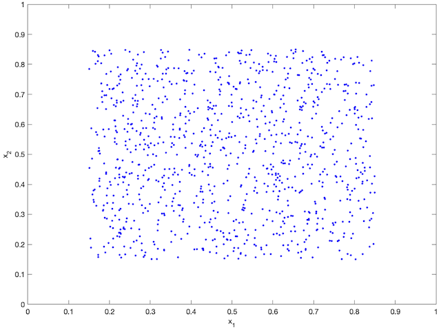
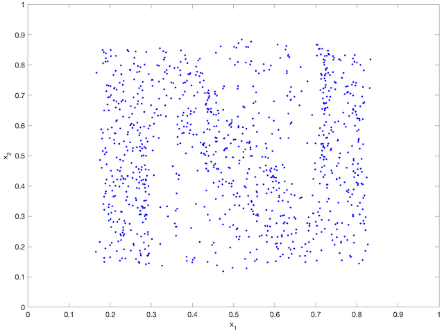
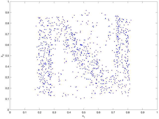
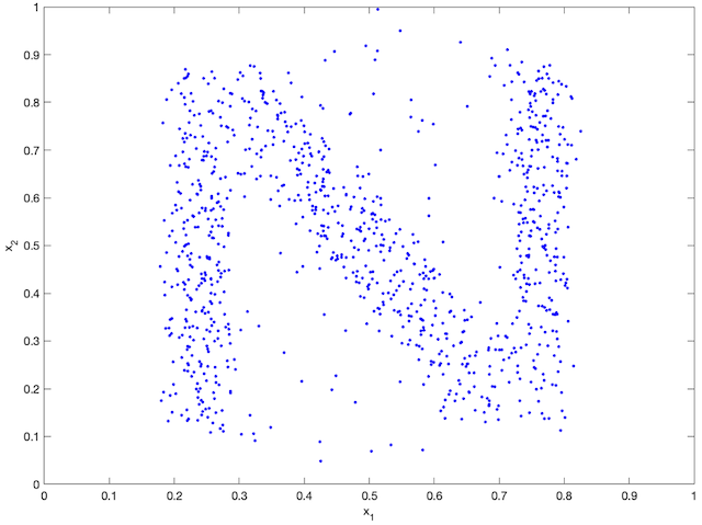
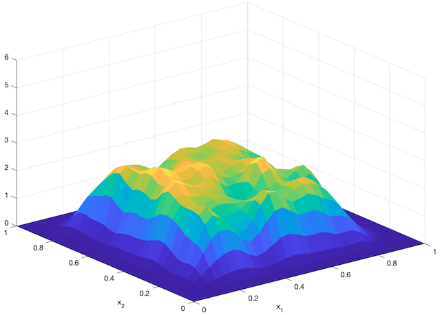
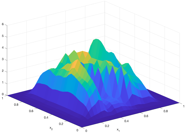
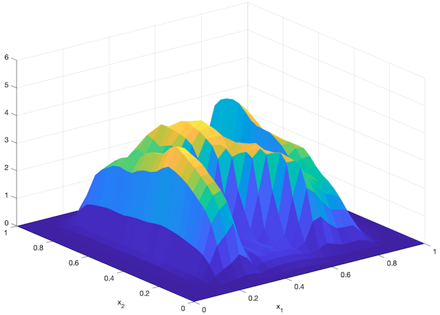
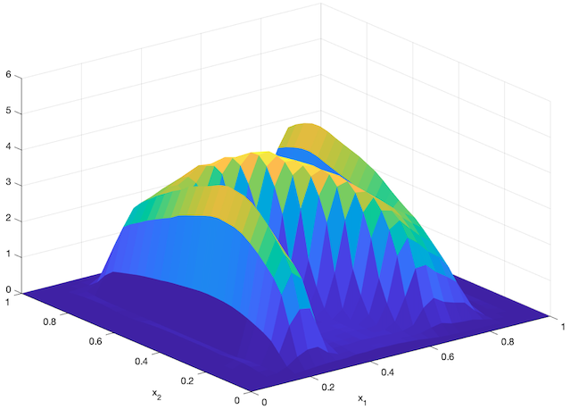
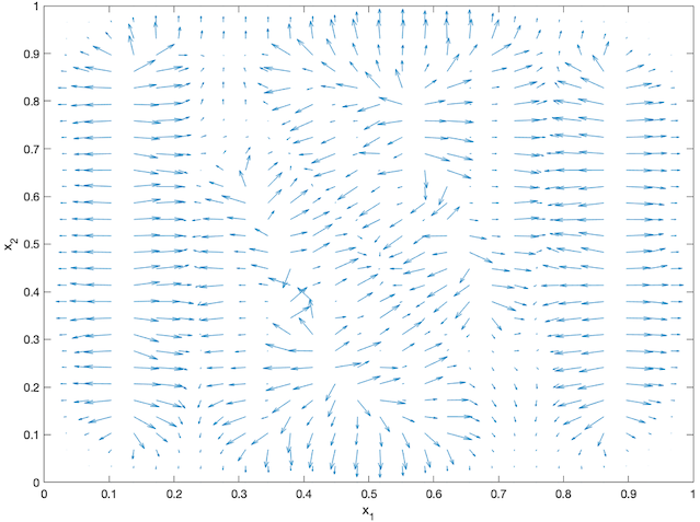
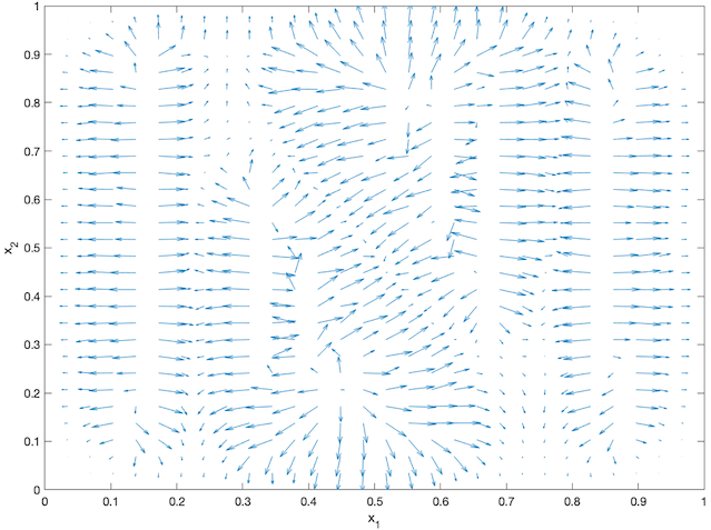
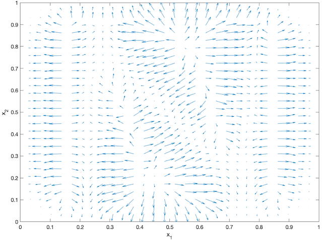
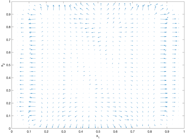
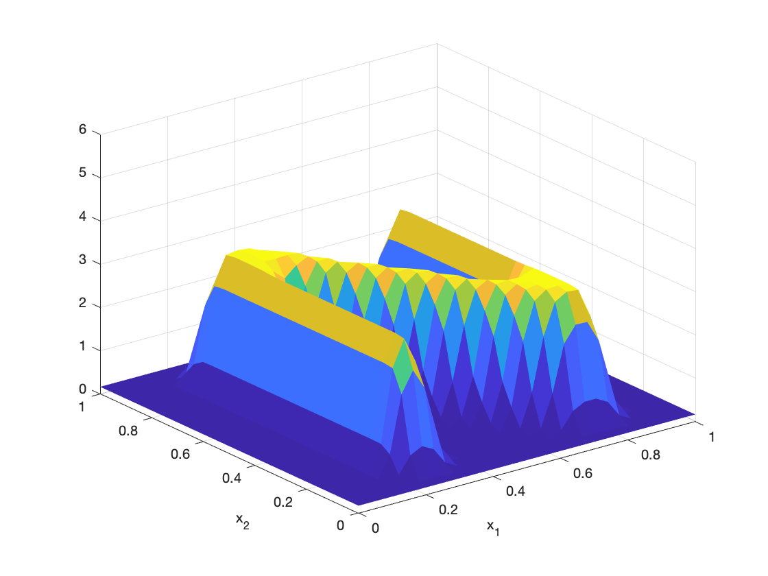
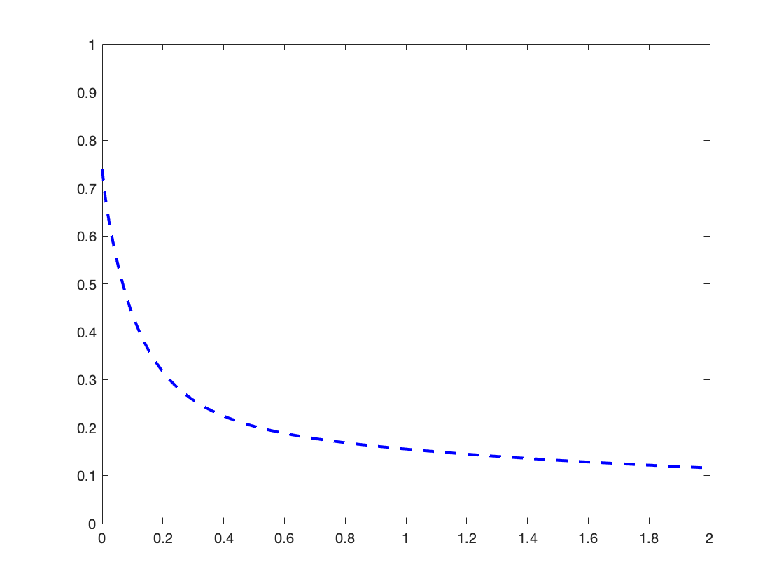
An agent-based simulation using 1024 robots is performed on Matlab to verify the proposed control law. We set , and . Each robot is simulated according to (2) where is given by (6). The initial positions are drawn from a uniform distribution on . The desired density is illustrated in Fig. 2(a). The implementation of the filters and the feedback controller is based on the finite difference method. We discretize into a grid, and the time difference is . We use KDE (in which we set ) to obtain and . Numerical implementation of the filters are introduced in [13]. Simulation results are given in Fig. 1. It is seen that the swarm is able to evolve towards the desired density. The convergence error is given in Fig. 2(b), which shows that the error converges exponentially to a small neighbourhood around and remains bounded, which verifies the ISS property of the proposed algorithm.
VI Conclusion
This paper studied the interplay of density estimation and control algorithms. We proposed new density feedback laws for robust density control of swarm robotic systems and filtering algorithms for estimating the mean-field density and its gradient. We also proved that the interconnection of these algorithms is globally ISS. Our future work is to incorporate the density control algorithm for higher-order nonlinear systems in [18] and the distributed density estimation algorithm in [13], and study their interconnected stability.
References
- [1] R. Olfati-Saber, J. A. Fax, and R. M. Murray, “Consensus and cooperation in networked multi-agent systems,” Proceedings of the IEEE, vol. 95, no. 1, pp. 215–233, 2007.
- [2] J. R. Marden, G. Arslan, and J. S. Shamma, “Cooperative control and potential games,” IEEE Transactions on Systems, Man, and Cybernetics, Part B (Cybernetics), vol. 39, no. 6, pp. 1393–1407, 2009.
- [3] M. Huang, R. P. Malhamé, P. E. Caines et al., “Large population stochastic dynamic games: closed-loop mckean-vlasov systems and the nash certainty equivalence principle,” Communications in Information & Systems, vol. 6, no. 3, pp. 221–252, 2006.
- [4] B. Açikmeşe and D. S. Bayard, “A markov chain approach to probabilistic swarm guidance,” in 2012 American Control Conference (ACC). IEEE, 2012, pp. 6300–6307.
- [5] S. Bandyopadhyay, S.-J. Chung, and F. Y. Hadaegh, “Probabilistic and distributed control of a large-scale swarm of autonomous agents,” IEEE Transactions on Robotics, vol. 33, no. 5, pp. 1103–1123, 2017.
- [6] K. Elamvazhuthi and S. Berman, “Optimal control of stochastic coverage strategies for robotic swarms,” in 2015 IEEE International Conference on Robotics and Automation (ICRA). IEEE, 2015, pp. 1822–1829.
- [7] Y. Chen, T. T. Georgiou, and M. Pavon, “Optimal steering of a linear stochastic system to a final probability distribution, part i,” IEEE Transactions on Automatic Control, vol. 61, no. 5, pp. 1158–1169, 2015.
- [8] J. Ridderhof, K. Okamoto, and P. Tsiotras, “Nonlinear uncertainty control with iterative covariance steering,” in 2019 IEEE 58th Conference on Decision and Control (CDC). IEEE, 2019, pp. 3484–3490.
- [9] U. Eren and B. Açıkmeşe, “Velocity field generation for density control of swarms using heat equation and smoothing kernels,” IFAC-PapersOnLine, vol. 50, no. 1, pp. 9405–9411, 2017.
- [10] K. Elamvazhuthi, H. Kuiper, M. Kawski, and S. Berman, “Bilinear controllability of a class of advection–diffusion–reaction systems,” IEEE Transactions on Automatic Control, vol. 64, no. 6, pp. 2282–2297, 2018.
- [11] T. Zheng, Q. Han, and H. Lin, “Transporting robotic swarms via mean-field feedback control,” IEEE Transactions on Automatic Control, pp. 1–1, 2021.
- [12] ——, “Pde-based dynamic density estimation for large-scale agent systems,” IEEE Control Systems Letters, vol. 5, no. 2, pp. 541–546, 2020.
- [13] ——, “Distributed mean-field density estimation for large-scale systems,” IEEE Transactions on Automatic Control, pp. 1–1, 2021.
- [14] D. Bakry, I. Gentil, and M. Ledoux, Analysis and geometry of Markov diffusion operators. Springer Science & Business Media, 2013, vol. 348.
- [15] S. Dashkovskiy and A. Mironchenko, “Input-to-state stability of infinite-dimensional control systems,” Mathematics of Control, Signals, and Systems, vol. 25, no. 1, pp. 1–35, 2013.
- [16] H. K. Khalil and J. W. Grizzle, Nonlinear systems. Prentice hall Upper Saddle River, NJ, 2002, vol. 3.
- [17] R. F. Curtain, “Infinite-dimensional filtering,” SIAM Journal on Control, vol. 13, no. 1, pp. 89–104, 1975.
- [18] T. Zheng, Q. Han, and H. Lin, “Backstepping density control for large-scale heterogeneous nonlinear stochastic systems,” in 2022 American Control Conference (ACC), 2022.
- [19] G. M. Lieberman, Second order parabolic differential equations. World scientific, 1996.
- [20] P. A. Markowich and C. Villani, “On the trend to equilibrium for the fokker-planck equation: an interplay between physics and functional analysis,” Mat. Contemp, vol. 19, pp. 1–29, 2000.
- [21] T. Cacoullos, “Estimation of a multivariate density,” Annals of the Institute of Statistical Mathematics, vol. 18, no. 1, pp. 179–189, 1966.