FedRN: Exploiting k-Reliable Neighbors Towards Robust Federated Learning
Abstract.
Robustness is becoming another important challenge of federated learning in that the data collection process in each client is naturally accompanied by noisy labels. However, it is far more complex and challenging owing to varying levels of data heterogeneity and noise over clients, which exacerbates the client-to-client performance discrepancy. In this work, we propose a robust federated learning method called FedRN, which exploits -reliable neighbors with high data expertise or similarity. Our method helps mitigate the gap between low- and high-performance clients by training only with a selected set of clean examples, identified by a collaborative model that is built based on the reliability score over clients. We demonstrate the superiority of \algname via extensive evaluations on three real-world or synthetic benchmark datasets. Compared with existing robust methods, the results show that \algname significantly improves the test accuracy in the presence of noisy labels.
1. Introduction
Federated learning (FL) is a privacy-preserving distributed learning technique, which handles a large corpus of decentralized data residing on multiple clients such as mobile or IoT devices (Bonawitz et al., 2019; Yang et al., 2021a). The main idea is to learn a joint model by alternating local update and model aggregation phases. Each client performs the local update phase by training the current model with its own training data without sharing any of the clients’ raw training data. Then, the model aggregation phase is executed by a server that merges received local models (McMahan et al., 2017). As the need for on-device machine learning is rising, FL has attracted much attention in various fields (Yang et al., 2021b; Chen et al., 2021; Muhammad et al., 2020; Jiang et al., [n. d.]; Luo et al., [n. d.]; Zhang et al., [n. d.]) and there have been numerous attempts to deploy it to on-device services, such as query suggestion for Google Keyboard (Yang et al., 2018) and question answering for Amazon Alexa (Chen et al., 2022).

(a) FedAvg. (b) Co-teaching. (c) \algname.

(a) Local Update Phase. (b) Model Aggregation Phase.
Since the FL system is deployed over heterogeneous networks, robustness has become an important challenge of federated learning, because the data collection process in each client is naturally accompanied by noisy labels, which may be corrupted from the ground-truth labels (Lee et al., 2021). In the presence of noisy labels, deep neural networks (DNNs) easily overfit to the noisy labels, thereby leading to poor generalization on unseen data (Zhang et al., 2017). Extensive efforts have been devoted to overcoming noisy labels in the centralized scenario (Xia et al., 2019; Li et al., 2020), but have yet to be studied widely in the federated learning (decentralized) scenario. Handling noisy labels in the FL scenario is far more challenging than in the centralized scenario, particularly on the following two difficulties:
-
(1)
Data Heterogeneity: Each client has non-independent and identically distributed (Non-IID) data with respect to the number of training examples for each class, which differ between clients.
-
(2)
Varying Label Noise: Noise ratios and types of data flaws vary between clients depending on how their data was collected, mainly attributed to the malfunction of data collectors, crowd-sourcing, and adversarial attacks.
As shown in Figure 1(a), these two difficulties exacerbate the performance discrepancy over clients because local data in each client varies in terms of data heterogeneity and label noise. Such a large performance discrepancy arguably results in poor performance of the global model, because client models are aggregated regardless of whether their models are corrupted from label noise (Chen and Chao, 2021).
The small-loss trick, which updates a DNN with a certain number of small-loss examples every training iteration (Jiang et al., 2018; Yu et al., 2019; Song et al., 2021; Han et al., 2018), could be a prominent direction to provide robustness; small-loss examples are typically regarded as the clean set because DNNs tend to first learn from clean data and then gradually overfit to noisy data (Arpit et al., 2017). However, as can be seen from Figure 1(b), the performance discrepancy still remains even when all the local models were trained using a popular robust learning method, Co-teaching (Han et al., 2018), that uses the small-loss trick for sample selection. Although the overall performance is higher than that of FedAvg, the performance gap between the high- and low-performance model is considerably large. Therefore, it is essential to not only (i) identify clean examples from noisy data, but also (ii) improve the low-performance models to increase the overall robustness for federated learning with noisy labels.
In this paper, we propose a simple yet effective robust approach called \algname (Fed-erated learning with Reliable Neighbors), which exploits -reliable neighbors in the client pool to help identify clean examples even when the target client is unreliable. We introduce the notion of k-reliable neighbors, which are clients that have similar data class distributions to the target client (data similarity), or minimal label noise in their data (data expertise). Using -reliable neighbors, \algname improves the performance of every client’s local model; the low-performance models benefit more from their -reliable neighbors, as shown in Figure 1(c).
In the local update phase shown in Figure 2(a), \algname first retrieves -reliable neighbors from the server. “Neighbor 2” has a relatively clean dataset or a similar class distribution to the target client’s, so the server transmits the model of “Neighbor 2” to the target client. The retrieved -reliable models are used to identify clean examples from the client’s dataset collaboratively with the target model; hence, with clear guidance from reliable neighbors, the target model can be improved significantly even if its performance is poor due to heavy label noise. In detail, the target and -reliable models fit bi-modal univariate Gaussian mixture models (GMMs) to the loss distribution of the target’s training data, respectively. Next, we build joint mixture models by aggregating all the GMMs based on the reliability scores of neighbor clients. Since the loss distributions of clean and noisy examples are bi-modal (Arpit et al., 2017), the training examples with a higher probability of belonging to the clean (i.e., small-loss) modality are treated as clean examples and used to robustly update the target model. In this process, the low-performance model hardly hinders the accuracy of sample selection due to its low reliability score.
After the local update phase, the weights of updated models are averaged to build a global model in the model aggregation phase in Figure 2(b). These two phases are repeated until the global model converges following the standard federated learning pipeline (McMahan et al., 2017).
Our main contributions are summarized as follows:
-
•
This is a new FL framework that exploits reliable neighbors to tackle the challenge of data heterogeneity and varying label noise.
-
•
We introduce and examine the two indicators of data expertise and similarity, measuring the reliability score of neighbor clients without infringing on data privacy.
-
•
\algname
remarkably improves the performance of underperforming client models by mitigating the client-to-client discrepancy, thereby boosting overall robustness.
-
•
\algname
significantly outperforms state-of-the-art methods on three real-world or synthetic benchmark datasets with varying levels of data heterogeneity and label noise.
2. Related Work
Federated Learning. Federated learning aims to learn a strong global model by exploiting all of the client data without infringing on data privacy. However, due to the heterogeneity in training data, it typically suffers from performance degradation of the global model (Zhu et al., 2021) or weight divergence (Zhao et al., 2018). In this regard, extensive efforts have been made to address these issues. Duan et al. (2019) addressed the problem of long-tailed distribution in training data by performing data augmentation. Zhao et al. (2018) let all of the clients share the same public data to mitigate the data heterogeneity. Meanwhile, Li et al. (2018) and Acar et al. (2020) added a regularization term that prevents the local model from diverging to the global model due to its own skewed Non-IID data. Although this family of methods contributes to improving the effectiveness of federated learning, they simply assume that all the labels in training data are clean, which is not a realistic scenario.
Learning with Noisy Labels. Extensive studies have been conducted to overcome noisy labels in the centralized scenario. A prominent direction for handling noisy labels is sample selection, which trains DNNs for a possibly clean subset of noisy training data. For example, Co-teaching (Han et al., 2018) trains two DNNs where each DNN selects small-loss examples in a mini-batch and then feeds them to its peer network for further training. MORPH (Song et al., 2021) divides the training process into two learning periods and employs two different criteria for sample selection. Another possible direction is to modify the loss of training examples based on importance reweighting or label correction (Patrini et al., 2017; Huang et al., 2020; Tanaka et al., 2018; Zheng et al., 2021).
Most recently, to leverage all the training data, sample selection methods have been combined with other approaches, such as loss correction and semi-supervised learning. SELFIE (Song et al., 2019) uses relabeled noisy examples in conjunction with the selected clean ones. DivideMix (Li et al., 2020) treats selected clean examples as labeled data and applies MixMatch (Berthelot et al., 2019) for semi-supervised learning. Despite these methods’ success, they do not perform well in the federated learning setting due to the client-to-client performance discrepancy.
Robust Federated Learning. To address the noisy labels in FL, most studies assume that trustworthy data exists either on the client- or server-side. Chen et al. (2020) estimated the credibility of each client with small clean validation data, and aggregated models based on the estimated credibilities of clients. Tuor et al. (2020) proposed a data filtering method, which identifies highly relevant examples for the given specific task using a reference model trained on clean benchmark data. In another direction, a few robust methods using label correction have been proposed (Yang et al., 2022; Zeng et al., 2022; Xu et al., 2022). The most representative Robust FL (Yang et al., 2022) shares the central representations of clients’ local data to maintain the consistent decision boundary over clients, and performed global-guided label correction assuming the IID scenario. However, existing methods often rely on unrealistic assumptions including the existence of clean validation data or the IID scenario. The recent label correction approaches including Robust FL still suffer from false label corrections produced by incorrect models under heavy label noise or severe Non-IID scenarios.
Difference from Existing Work. We clarify why FL with noisy labels is problematic; the client-to-client performance discrepancy hinders the use of existing robust methods in the label noise community into FL. Although a few robust methods have been proposed, this problem has been overlooked. In this paper, we thus bridge the two different topics to improve overall robustness by introducing -reliable neighbors such that they deliver credible information to the clients. Moreover, compared to all aforementioned robust methods, \algname mainly focuses on identifying reliable neighbor clients for sample selection, which does not require any unrealistic supervision, such as a clean validation set or knowledge of true noise rates per client.
3. Preliminaries
A multi-class classification problem requires training data , where is a training example with its ground-truth label . However, noisy training data may have corrupted labels such that for some . We herein briefly summarize the conventional learning pipeline for (i) standard federated learning and (ii) robust learning with sample selection.
-
•
Federated Learning (FedAvg): It is assumed that each client has its own Non-IID dataset (i.e., ), and cannot directly access another client’s data. Therefore, a global model is trained by alternating the local update and model aggregation phase.
During the local update phase, a fixed number of target clients are selected from the entire client pool. For each target client , all the other clients are defined as its neighbors . Next, the target client’s local model is trained on its own data for certain local epochs with the standard stochastic gradient decent (McMahan et al., 2017). All the trained models for are then received and averaged by the server in the model aggregation phase,
(1) where is the aggregation weight that is based on the data size of each client. Lastly, the updated global model is broadcasted to the clients. This training round is called a transmission round and is repeated until convergence.
-
•
Robust Learning with Sample Selection: Many recent robust approaches have adopted sample selection, which treats a certain number of small-loss examples as the clean set (Han et al., 2018; Yu et al., 2019; Li et al., 2020; Song et al., 2021). In the centralized scenario, given a noisy mini-batch (), the clean subset is identified and used to directly update the global model ,
(2) where is the learning rate and is a certain loss function. The remaining examples (mostly large-loss examples) in the mini-batch are excluded to pursue robust learning.
Note that training data is typically assumed to be clean in federated learning, while a global model is assumed to have access to all of the training data in robust learning. However, our objective is to robustly train a global model even when noisy labels exist in the federated learning scenario.
4. Proposed Method: FedRN
We introduce the notion of -reliable neighbors and describe how to leverage them for robust federated learning with noisy labels.
4.1. Main Concept: k-Reliable Neighbors
The key idea of \algname is to exploit useful information in other clients without violating privacy. Hence, the main challenge is to find the most helpful neighbor clients using limited information about each client. Intuitively speaking, these helpful neighbor clients have (1) high expertise on their data, or (2) data distributions similar to the target client’s:
-
•
Data Expertise: The training data should be sufficiently clean. The neighbor client with heavy noise could hinder identifying clean examples from the client’s noisy data.
-
•
Data Similarity: Data and class distributions should be similar to the target client’s. The distribution shift problem could lead to model incompatibility between target and neighbor clients.
We investigate how these two considerations affect selecting reliable neighbor clients for robust federated learning. Given a target client , a reliable neighbor client is defined to be one of the -reliable neighbors , as described in Definition 3. Satisfying the condition, -reliable neighbors can deliver clean and useful information even when the training data of the target client is unreliable due to the heavy label noise.
Definition 4.1.
Let and be the score function for data expertise of a client and data similarity between two clients, respectively. Given a target client and available neighbor clients , the -reliable neighbors is a subset of with size satisfying,
| (3) |
and is the balancing term that determines the contribution of each score. The data similarity to itself is 1, i.e., . ∎
To compute the reliability score in Eq. (3), we propose two indicators of data expertise and similarity using client’s local models. Since it is infeasible to access the raw data in neighbor clients, we leverage the server’s copies of local models, which are sent to the server during the model aggregation phase. By doing so, our approach does not compromise the privacy-preserving property in federated learning.
With the intention of selecting clients with cleaner examples, we define the data expertise score motivated by the memorization effect of DNNs. In general, DNNs memorize clean examples faster than noise examples during training, which has been observed consistently even at extreme noise ratios (Song et al., 2021). In this sense, the early memorization of clean examples leads to higher training accuracy if the client has cleaner local data. Consequently, during the model aggregation phase, the server receives the training accuracy of each client along with their local models, then computes and normalizes the data expertise Exp() per client,
| (4) |
where denotes the training accuracy of the local model for the client ; and are the maximum and minimum training accuracy of the given client set.
Regarding the data similarity score, we propose to use predictive difference, which provides a hint to the similarity between two heterogeneous data distributions without the use of raw data. Hence, the data similarity between two clients is approximated by the prediction difference for the same random input, where a smaller difference indicates a higher similarity. Accordingly, after the local update phase, each client generates the same input of Gaussian random noise (Jeong et al., 2021) and transmits its softmax outputs into the server, where denotes the softmax output of the client for input . The data similarity Sim() between the target client and neighbor client is then computed by the server,
| (5) |
We use the cosine similarity denoted by Cosine to measure the predictive difference, because the symmetry of similarity is guaranteed, i.e., . The min-max normalization is also applied similarly to data expertise. We provide an in-depth analysis of how the two proposed indicators work precisely in Section 5.4.
4.2. Robust Learning with k-Reliable Neighbors
For every communication round, each client participating in the upcoming round receives its -reliable neighbors from the server. When updating the target client’s model, we follow the general philosophy of sample selection for robust learning by identifying clean examples from the noisy training data.
Different to robust methods in centralized scenarios, models, comprising -reliable neighbors and the target client’s model, cooperate to mitigate the performance discrepancy among clients and obtain more reliable results. For each of the models, we fit two-component GMMs to model the loss distributions of clean and noisy examples in view of loss distributions being bi-modal (Li et al., 2020; Arazo et al., 2019). Based on the ensembled results of these GMMs, the target client’s model is only updated with examples selected as clean.
To be specific, our aim is to estimate the probability of each training example being clean with models with different reliability scores. At the beginning of the local update phase, the GMM is fitted to the loss of all available training examples in the target client by using the Expectation-Maximization (EM) algorithm. Given a noisy example , the probability of being clean is obtained through its posterior probability for the clean (small-loss) modality,
| (6) |
where g denotes the Gaussian modality with a smaller mean (i.e., smaller loss) and is the loss function. Subsequently, the probability of each example to be clean is ensembled over models with their reliability scores in Eq. (3). Given a target client , the clean probability of joint mixtures can be formulated as:
| (7) |
The ensemble with the reliability scores give higher weight to the GMMs of trusted neighbors with high data expertise or similarity.
Lastly, \algname constructs a clean set such that each training example in the set has a clean probability greater than ,
| (8) |
where is the noisy data of the target client . The model is finally updated with only the clean set for a specified number of local epochs in the local update phase, while the complement of the set, which are likely to be noisy, are discarded for robust learning.
This collaborated approach with -reliable neighbors considerably increases the robustness of low-performance clients with the aid of neighbors with high data expertise or similarity. Therefore, \algname reduces the performance gap between clients and enhances the overall robustness, thus leading to a stronger global model.
4.3. Fine-tuning with k-Reliable Neighbors
Due to the data heterogeneity in federated learning, the problem of distribution shift between clients’ local models is another challenge when ensembling their predictions for sample selection. Hence, \algname is integrated with the fine-tuning technique that helps quickly adapt to the local data distribution (Collins et al., 2021).
Before constructing the clean set in Eq. (8), we identify an auxiliary set of clean examples using only the target client’s model,
| (9) |
and fine-tune all the retrieved -reliable neighbors for the auxiliary set. The auxiliary set could, however, be very noisy especially when the target client has heavy noise in its training data. To prevent feature extractors from being corrupted by such client-side noise, we only fine-tune the classification head. In Section 5.5, we examine the effect of the fine-tuning technique on data expertise and similarity used in neighbor search, and provide insights on their use for robust federated learning with noisy labels.
4.4. Algorithm Pseudocode
Input: : noisy data of client , : total rounds,
: local epochs, : reliable neighbors
Output: : a global model
Algorithm 1 describes the overall procedure of \algname. We perform standard federated learning, FedAvg, for warm-up epochs before applying \algname, because robust training methods are generally applied after the warm-up phase in the literature (Han et al., 2018; Song et al., 2019). When training with \algname, retrieved neighbor models are fine-tuned for 1 epoch before sample selection (Line 11). Next, the target client identifies clean examples by leveraging -reliable neighbor models (Line 13). The received global model is updated with estimated clean samples (Lines 14–15). In the aggregation phase, the central server aggregates the updated local models (Line 20).
The main additional cost of \algname is the communication overhead from sending -reliable models from the server to the selected client (see Appendix 5.9 for detailed cost analysis). However, a small number of reliable neighbors is sufficient (see Section 5.6) and the cost can be drastically reduced by over a factor of 32 times in modern federated learning by sending the difference of parameters (Jeong et al., 2021) or a compressed model (Malekijoo et al., 2021). Furthermore, there is no issues in model convergence because we applied a sample selection approach, which don’t has convergence problems, in a decentralized setting using FedAvg (McMahan et al., 2017), which has proven model convergence.
5. Evaluation
Our evaluation was conducted to support the following:
-
•
\algname
is more robust than five state-of-the-art methods for federated learning with noisy labels (Section 5.2).
-
•
\algname
consistently identifies clean examples from noisy data with high precision and recall (Section 5.3).
-
•
The reliability metric is effective in finding -reliable neighbors for robust learning (Section 5.4).
-
•
The use of fine-tuning is necessary owing to the distribution shift in local data (Section 5.5).
-
•
A small number ( of reliable neighbors is sufficient to achieve high robustness (Section 5.6).
5.1. Experiment Configuration
We verified the superiority of \algname compared with five robust learning methods on three real-world or synthetic benchmark datasets in a Non-IID federated learning setting, where the Non-IID setting is more realistic and difficult than the IID setting (Zhu et al., 2021; Zhao et al., 2018; Briggs et al., 2020).
Datasets. We performed image classification on synthetic and real-world benchmark data: CIFAR-10 and CIFAR-100; mini-WebVision, a subset of real-world noisy data consisting of large-scale web images. We used the first 50 classes in WebVision V1 following the literature (Li et al., 2020). The statistics of them are summarized in Table 1.
| # of Train | # of Val. | # of Classes | Noise Ratio | |
|---|---|---|---|---|
| CIFAR-10 | 50,000 | 10,000 | 10 | |
| CIFAR-100 | 50,000 | 10,000 | 100 | |
| mini-WebVision | 65,944 | 2500 | 50 |
| Non-IID Type | Shard () | Shard () | Dirichlet () | |||||||||
|---|---|---|---|---|---|---|---|---|---|---|---|---|
| Noise Type | Symmetric | Asym | Mixed | Symmetric | Asym | Mixed | Symmetric | Asym | Mixed | |||
| Noise Rate | 0.0–0.4 | 0.0–0.8 | 0.0–0.4 | 0.0–0.4 | 0.0–0.4 | 0.0–0.8 | 0.0–0.4 | 0.0–0.4 | 0.0–0.4 | 0.0–0.8 | 0.0–0.4 | 0.0–0.4 |
| Oracle111 | 69.10 | 67.19 | 69.10 | 68.89 | 78.00 | 75.94 | 78.00 | 77.7 | 81.79 | 80.38 | 81.79 | 81.39 |
| FedAvg (McMahan et al., 2017) | 46.39 | 38.69 | 49.09 | 46.82 | 66.44 | 56.46 | 67.23 | 67.95 | 75.92 | 70.60 | 77.77 | 77.17 |
| Co-teaching (Han et al., 2018) | 63.20 | 52.72 | 62.48 | 61.68 | 74.66 | 67.17 | 74.18 | 75.18 | 79.97 | 75.39 | 79.53 | 79.94 |
| Joint-optm (Tanaka et al., 2018) | 50.44 | 42.23 | 38.04 | 47.28 | 69.22 | 64.02 | 67.29 | 68.84 | 75.46 | 70.43 | 74.81 | 75.43 |
| SELFIE (Song et al., 2019) | 62.64 | 53.69 | 64.21 | 62.63 | 74.57 | 66.90 | 74.77 | 74.44 | 78.57 | 72.92 | 78.58 | 79.02 |
| DivideMix (Li et al., 2020) | 62.35 | 58.18 | 62.07 | 63.38 | 68.73 | 65.82 | 68.95 | 69.32 | 74.26 | 72.25 | 73.29 | 73.47 |
| Robust FL (Yang et al., 2022) | 56.25 | 45.59 | 55.52 | 57.58 | 70.30 | 62.89 | 69.04 | 70.02 | 75.75 | 70.63 | 74.00 | 75.49 |
| \algname (k=1) | 67.33 | 60.33 | 67.51 | 67.92 | 76.37 | 72.30 | 76.74 | 76.92 | 79.99 | 75.92 | 80.05 | 79.79 |
| \algname (k=2) | 67.62 | 62.94 | 68.33 | 68.11 | 76.81 | 72.85 | 77.33 | 76.99 | 80.34 | 76.49 | 80.38 | 80.28 |
| Non-IID Type | Shard () | |||
|---|---|---|---|---|
| Noise Type | Symmetric | Asym | Mixed | |
| Noise Rate | 0.0–0.4 | 0.0–0.8 | 0.0–0.4 | 0.0–0.4 |
| Oracle | 47.83 | 44.82 | 47.83 | 47.33 |
| FedAvg (McMahan et al., 2017) | 33.36 | 26.15 | 34.90 | 34.02 |
| Co-teaching (Han et al., 2018) | 43.43 | 37.05 | 42.90 | 43.83 |
| Joint-optm (Tanaka et al., 2018) | 35.89 | 30.92 | 33.15 | 35.29 |
| SELFIE (Song et al., 2019) | 44.14 | 37.65 | 43.25 | 43.78 |
| DivideMix (Li et al., 2020) | 46.21 | 42.83 | 45.59 | 46.94 |
| Robust FL (Yang et al., 2022) | 35.33 | 29.20 | 33.08 | 34.27 |
| \algname (k=1) | 47.30 | 42.27 | 47.62 | 46.62 |
| \algname (k=2) | 47.46 | 43.07 | 47.52 | 47.17 |
For the federated learning setup with noisy labels, we merged the standard setting in the two research communities:
-
•
Non-IID Data: Two popular ways of client data partitioning were applied (Zhu et al., 2021); (i) Sharding: training data is sorted by its class labels and divided into “” shards, which are randomly assigned to each client with an equal number of . (ii) Dirichlet Distribution: each client is assigned with training data drawn from the Dirichlet distribution with a concentration parameter . For the experiments, was set to , , , or , and was set to .
-
•
Label Noise: We injected artificial noise by following typical protocols (Song et al., 2022); (i) Symmetric Noise: a true label is flipped into all possible labels with equal probability. (ii) Asymmetric Noise: a true label is flipped into only a certain label. Note that we injected varying levels of label noise into the clients, so each client had different noise rates. For instance, a noise of – means that the noise rate increases linearly from to as the client’s index increases; thus, the average noise rate of clients’ training data is . We further tested for mixed noise where the two different types of label noise are injected into the clients. That is, symmetric noise is applied to half of the clients, while asymmetric noise is applied to the remaining clients.
We did not inject any label noise into mini-WebVision because it contains real label noise whose rate is estimated at (Song et al., 2022).
Implementation Details. We compared \algname with a standard federated learning method, FedAvg (McMahan et al., 2017), and five state-of-the-art robust methods for handling noisy labels, namely Co-teaching (Han et al., 2018), Joint-optimization (Tanaka et al., 2018), SELFIE (Song et al., 2019), DivideMix (Li et al., 2020), and Robust FL (Yang et al., 2022). All the robust methods were combined with FedAvg to support decentralized learning. The total number of clients was set to with a fixed participation rate of . The training (transmission) round was set to be for CIFAR-10 and for CIFAR-100 and WebVision, ensuring all the models’ training convergence. The SGD optimizer was used with a learning rate of and a momentum of . The number of local epochs was set to be . We used the model for learning consists of 4 convolution layers and 1 linear classifier for CIFAR-10 and MobileNet for CIFAR-100 and mini-WebVision.
As for hyperparameters related to our method, \algname requires the balancing term and number of reliable neighbors . We used , which was obtained via a grid search (see the section 5.7). We used and since the performance gain of \algname was consistently high as long as , which is detailed in Section 5.6.
The hyperparameters of the baseline robust methods were configured favorably in line with the literature. We clarify the hyperparmeter setup of all baseline algorithms, as follows:
-
•
Joint Optimization (Tanaka et al., 2018) requires the two coefficients for its two regularization losses for robust learning. These two coefficients were set to be 1.2 and 0.8, respectively.
-
•
SELFIE (Song et al., 2019) requires the uncertainty threshold and the length of label history as its hyperparameters. As suggested by the authors, they were set to be 0.05 and 15, respectively.
-
•
DivideMix (Li et al., 2020) applies MixMatch for semi-supervised learning, which requires the sharpening temperature, the unsupervised loss coefficient, and the Beta distribution parameter. They were set to be 0.5, 25, and 4, respectively.
-
•
Robust FL (Yang et al., 2022) requires two coefficients for its two additional regularization losses similar to Joint Optimization. They were set to be 1.0 and 0.8, respectively.
| Shard () | mini-WebVision | |
|---|---|---|
| Method | Top-1 Accuracy | Top-5 Accuracy |
| FedAvg (McMahan et al., 2017) | 20.80 | 45.00 |
| Co-teaching (Han et al., 2018) | 21.76 ( 0.96) | 46.64 ( 1.64) |
| Joint-optm (Tanaka et al., 2018) | 13.56 ( 7.24) | 35.56 ( 9.44) |
| SELFIE (Song et al., 2019) | 22.20 ( 1.40) | 48.76 ( 3.76) |
| DivideMix (Li et al., 2020) | 20.84 ( 0.04) | 45.72 ( 0.72) |
| Robust FL (Yang et al., 2022) | 14.12 ( 6.68) | 35.24 ( 9.76) |
| \algname (k=1) | 22.52 ( 1.72) | 48.48 ( 3.48) |
| \algname (k=2) | 22.76 ( 1.96) | 49.16 ( 4.16) |
All of the algorithms were implemented using PyTorch and executed using four NVIDIA RTX 2080Ti GPUs. In support of reliable evaluation, we repeated every task thrice and reported the average test (or validation) accuracy, which is the common measure of robustness to noisy labels (Han et al., 2018; Chen et al., 2019).

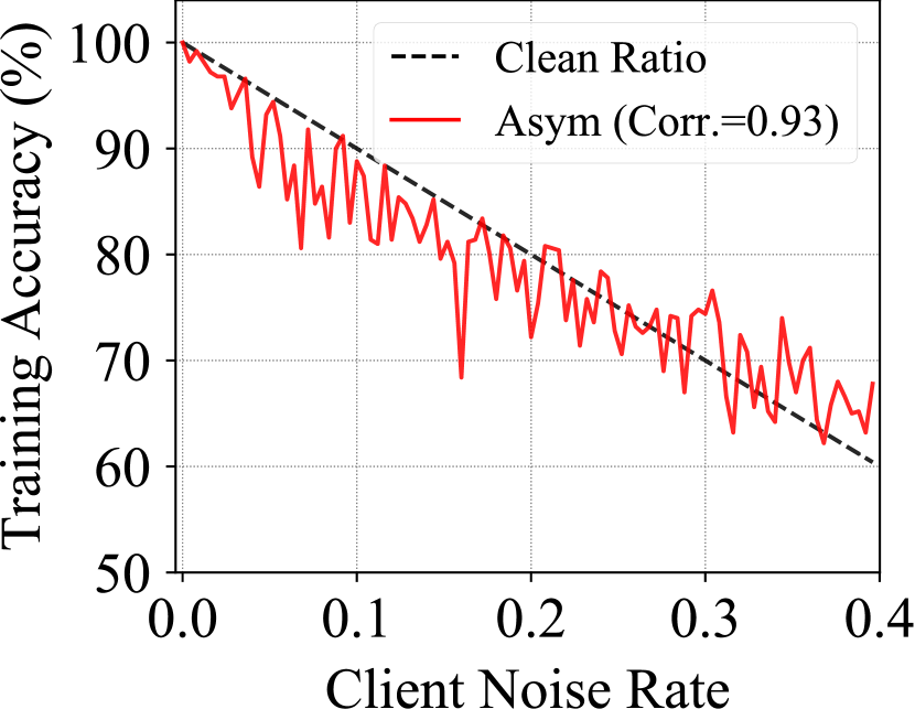
(a) Symmetric Noise of –. (b) Asymmetric Noise of –.
![[Uncaptioned image]](https://cdn.awesomepapers.org/papers/7cb4bae9-9f81-4d39-8e80-dc3b5fa5125b/x4.png)
(a) Symmetric Noise. (b) Asymmetric Noise.
5.2. Robustness Comparison
5.2.1. Results with Synthetic Noise
Tables 2 and 3 show the test accuracy of the global model trained by eight methods for three Non-IID federated learning scenarios with four different noise settings, including symmetric, asymmetric, and mixed label noise. Overall, \algname achieves the highest test accuracy in every case. Compared with FedAvg, \algname’s accuracy improves relatively more as the noise rate increases from – to – in symmetric noise, because the performance discrepancy over clients drastically degrades with the increase in noise rate. In contrast, the other robust methods show considerably poor performance compared with \algname, which is presumably attributed to the client-to-client performance discrepancy, despite the fact that they are incorporated with FedAvg. Meanwhile, the recent robust FL method, Robust FL, shows relatively poor performance in our setup since the method produces many false label corrections due to the clients with heavy label noise. Unlike, \algname is robust even to heavy noise because all unreliable labels are excluded from training for high safety without correction. Our method can be extended with semi-supervised learning for exploiting even unreliable examples. We leave this as future work.
5.2.2. Results with Real-world Noise
Table 4 displays the validation accuracy of seven different methods on a real-world noisy mini-WebVision dataset. We report the top-1 and top-5 classification accuracy on the mini-WebVision validation set. \algname maintains its performance dominance over multiple state-of-the-art robust methods for real-world label noise as well. \algname () improves the top-1 accuracy by up to compared with other robust methods.
![[Uncaptioned image]](https://cdn.awesomepapers.org/papers/7cb4bae9-9f81-4d39-8e80-dc3b5fa5125b/x6.png)

(a) w.o Label Noise. (b) w. Label Noise.
5.3. In-depth Analysis on Selected Examples
All methods except FedAvg and Joint Optimization follow the pipeline of learning with sample selection. Hence, we evaluate the sample selection performance of them using the two metrics, namely label precision (LP) and recall (LR), which respectively represent the quality and quantity of examples selected as clean (Han et al., 2018; Song et al., 2021),
empty
where and denote the training data and its selected clean set of the client , respectively.
Figure 3 shows the LP and LR curves averaged across all the clients per epoch on CIFAR-10 with symmetric and asymmetric label noise. The results of Robust FL are omitted due to its too low label precision and recall under the Non-IID scenario. After the warm-up period of transmission rounds, \algname shows the highest LP and LR with a large improvement of up to and , respectively. In addition, its dominance over other robust learning methods is consistent regardless of the noise type. Therefore, these results indicate that the superior robustness of \algname in Tables 2–4 is due to its high LP and LR.
5.4. In-depth Analysis on Reliability Metric
-
•
Data Expertise: Figure 4 shows the training convergence rate (training accuracy) of all clients sorted in ascending order by their noise rate. Owing to the memorization effect of DNNs, the training accuracy of the local model indeed has a strong correlation of over with respect to varying levels of label noise. These results confirm that the client’s training accuracy represents its data expertise.
-
•
Data Similarity: Figure 5 shows similarity matrices between client’s softmax outputs for a Gaussian random noise when trained on data with or without label noise. As clients with similar Ids (indices) have similar data distributions in our Non-IID setting, the similarity around diagonal entries is high, as can be seen from Figure 5(a). Even with label noise shown in Figure 5(b), it turns out that the similarity trend remains. Therefore, it can be concluded that the similarity between the softmax output is a robust metric to find clients with similar data distributions.
These empirical studies provide empirical evidence for the use of our two indicators, and .
5.5. Reliable Neighbors with Fine-tuning
We analyze the effect of fine-tuning on data expertise and similarity used in neighbor search. Table 5 summarizes the performance of \algname () with and without fine-tuning, where a small indicates that data similarity is considered more than data expertise. When fine-tuning is deactivated, the benefit of retrieving neighbors with high data similarity is remarkably dominant, because lower data similarity implies a larger distribution shift between the target and neighbor models. On the other hand, an opposite trend is observed when fine-tuning is activated. The test accuracy is high when data expertise is properly considered in conjunction with data similarity. Overall, fine-tuning does not only help mitigate the distribution shift problem but also significantly improves performance of \algname.
| w.o. Fine-tuning | w. Fine-tuning | |||
|---|---|---|---|---|
| 0.0–0.4 | 0.0–0.8 | 0.0–0.4 | 0.0–0.8 | |
| 0.0 | 65.03 | 58.20 | 67.11 | 61.81 |
| 0.2 | 63.77 | 57.24 | 67.45 | 62.69 |
| 0.4 | 62.45 | 53.89 | 67.03 | 62.94 |
| 0.6 | 58.74 | 51.36 | 67.62 | 62.94 |
| 0.8 | 56.60 | 43.61 | 67.19 | 62.97 |
| 1.0 | 56.06 | 44.87 | 66.73 | 61.61 |
5.6. Ablation Study on k-Reliable Neighbors
| Shard () | Dirichlet () | |||
|---|---|---|---|---|
| 0.0–0.4 | 0.0–0.8 | 0.0–0.4 | 0.0–0.8 | |
| 1 | 67.33 | 60.33 | 79.99 | 75.92 |
| 2 | 67.62 | 62.94 | 80.34 | 76.49 |
| 3 | 68.10 | 62.77 | 80.31 | 76.01 |
| 4 | 67.38 | 62.75 | 80.36 | 76.16 |
| 5 | 67.60 | 63.10 | 80.18 | 76.00 |
| Shard () | ||||
| Symmetric | Asym | Mixed | ||
| 0.0–0.4 | 0.0–0.8 | 0.0–0.4 | 0.0–0.4 | |
| 1 | 47.30 | 42.27 | 47.62 | 46.62 |
| 2 | 47.46 | 43.07 | 47.52 | 47.17 |
| 3 | 47.65 | 42.33 | 48.18 | 47.01 |
| 4 | 47.66 | 42.48 | 47.55 | 47.72 |
| 5 | 48.10 | 42.58 | 47.43 | 47.40 |
| Communication | Computation | |||||
|---|---|---|---|---|---|---|
| ServerClient | ClientServer | Total Cost | Forward | Backward | Total Cost | |
| FedAvg (McMahan et al., 2017) | M | M | ||||
| Co-Teaching (Han et al., 2018) | ||||||
| Joint-optm (Tanaka et al., 2018) | M | M | ||||
| SELFIE (Song et al., 2019) | M | M | ||||
| DivideMix (Li et al., 2020) | ||||||
| Robust FL (Yang et al., 2022) | M | M | ||||
| FedRN | M | |||||
A larger number of reliable neighbors could increase the communication overhead in federated learning. We, therefore, investigated the change in performance of the global model according to the the number of reliable neighbors. Tables 6 and 7 show the classification accuracy on CIFAR-10 and CIFAR-100 respectively with varying number of neighbors. The results show that \algname with and generally shows comparable performance than ; there is little improvement in performance with the increase in the number of reliable neighbors as long as . In other words, using only one or two reliable neighbors is sufficient to improve the robustness, because the proposed reliability score successfully retrieves the most helpful neighbor client among all the neighbors. Therefore, in a scenario where the communication burden is significant, practitioners may reduce the communication overhead by only using a single reliable neighbor with \algname to handle the problem of noisy labels.
5.7. Grid Search for Balancing Term
We adjusted to determine the contribution of data expertise and similarity in neighbor search. To ascertain the optimal value, we repeated the experiment on CIFAR-10 with various values, as summarized in Table 10. Because the fine-tuning technique is incorporated in \algname, merging data expertise and similarity provides a synergistic enhancement in general. In particular, when , the performance gain is the highest on average. Based on these results, we set to for all experiments in Section 5.
| Symmetric Noise | ||||||
| Type | Shard () | Shard () | Dirichlet | |||
| 0.0–0.4 | 0.0–0.8 | 0.0–0.4 | 0.0–0.8 | 0.0–0.4 | 0.0–0.8 | |
| -random | 66.82 | 60.11 | 76.37 | 71.56 | 79.79 | 75.11 |
| -reliable | 67.62 | 62.94 | 76.81 | 72.85 | 80.34 | 76.49 |
5.8. Comparison with Random Neighbors
We analyzed the usefulness of -reliable neighbors compared with -random neighbors. For -random neighbors, we replaced Lines 6 and 10 of Algorithm 1 with random client selection. Table 9 summarizes the test accuracy of \algname with -reliable and -random neighbors. Since our fine-tuning technique was incorporated with -random neighbors, using -random neighbors improves the robustness against noisy labels, but \algname with -reliable neighbors maintains its dominance in every case. In detail, if the neighbors with low data expertise are selected, they misclassify mislabeled examples as clean examples in sample selection. Likewise, the neighbors with significantly different data distributions harm identifying clean examples from the target client’s noisy data due to the distribution shift problem. It can be confirmed experimentally that this issue becomes more prominent when the noise rate is high. In conclusion, we should leverage the reliability of neighbors to obtain a global model robust to noisy labels.
5.9. Detailed Cost Analysis
We analyze the communication and computation cost of \algname compared with other six methods, as summarized in Table 8. In this comparison, the communication cost is split into two parts, “serverclient” and “clientserver,” while the computation cost is split into two other parts, “forward” and “backward,” and the “total cost” aggregates all the costs for each perspective.
| Shard () | Dirichlet () | ||||
|---|---|---|---|---|---|
| 0.0–0.4 | 0.0–0.8 | 0.0–0.4 | 0.0–0.8 | Mean | |
| 0.0 | 67.11 | 61.81 | 80.18 | 75.94 | 71.26 8.33 |
| 0.2 | 67.45 | 62.69 | 80.35 | 75.95 | 71.61 8.00 |
| 0.4 | 67.03 | 62.94 | 79.95 | 76.27 | 71.55 7.90 |
| 0.6 | 67.62 | 62.94 | 80.34 | 76.49 | 71.85 7.97 |
| 0.8 | 67.19 | 62.97 | 80.18 | 76.28 | 71.76 7.80 |
| 1.0 | 66.73 | 61.61 | 80.00 | 76.07 | 71.10 8.43 |
-
•
Communication Cost: \algname requires 3M or 4M communication cost in total when using one or two reliable neighbors, which is a sufficient number for general use cases. The remaining communication cost for calculating data similarity and expertise (i.e., and ) is negligible. By contrast, Co-Teaching and DivideMix both require 4M communication cost in total because they maintain two models for co-training. In summary, \algname leads to greater performance with comparable or lower communication cost compared with other baseline methods.
-
•
Computation Cost: We exclude the cost of fitting GMMs and searching -reliable neighbors because their costs are negligible compared to those of the forward and backward steps. Along the pipeline of our local update phase, \algname first requires F and B computation cost to perform fine-tuning with -reliable neighbors for one epoch. Next, to construct the clean set, F communication cost is needed due to the inference with available models. As the constructed clean set is deterministic over all the local epochs, only F+B computation cost is required to train a single model for the given local epoch in each communication round. Consequently, \algname needs F + B computation cost in total. In a typical deep learning pipeline, the cost of the backward step is relatively smaller than that of the forward step. Hence, the computation cost for the forward step is the major issue. In light of this fact, the forward cost of \algname is comparable to those of FedAvg, Joint-optim, and SELFIE, and less than those of Co-teaching and DivideMix, because the number of local epochs is larger than the number of reliable neighbors, . Among the compared methods, DivideMix is the slowest method in that it performs data augmentations with two models for each local epoch, so its forward cost is F.
Therefore, with one or two reliable neighbors, \algname greatly improves the robustness of the global model without adding much communication and computation cost in the scenario of federated learning with noisy labels.
6. Conclusion
The scenario of considering both data heterogeneity and label noise is a new important research direction of practical federated learning. In this paper, we propose a novel federated learning method called FedRN. In the local update phase, -reliable neighbors with high data expertise or similarity are retrieved, and they identify clean examples collaboratively based on their reliability scores. The models are then trained on the clean set, and the weights are averaged in the model aggregation phase. As a result, \algname achieves high label precision and recall for sample selection, leading to a robust global model even in the presence of label noise. We conducted extensive experiments on three real-world or synthetic noisy datasets. The results verified that \algname improves the robustness against label noise consistently and significantly. Overall, the use of reliable neighbors will inspire future studies for robustness.
7. Acknowledgement
This work was supported by Institute of Information & communications Technology Planning & Evaluation (IITP) grant funded by the Korea government(MSIT) (No.2019-0-00075, Artificial Intelligence Graduate School Program(KAIST) and No. 2022-0-00871, Development of AI Autonomy and Knowledge Enhancement for AI Agent Collaboration)
References
- (1)
- Acar et al. (2020) Durmus Alp Emre Acar, Yue Zhao, Ramon Matas, Matthew Mattina, Paul Whatmough, and Venkatesh Saligrama. 2020. Federated learning based on dynamic regularization. In ICLR.
- Arazo et al. (2019) Eric Arazo, Diego Ortego, Paul Albert, Noel O’Connor, and Kevin McGuinness. 2019. Unsupervised label noise modeling and loss correction. In ICML.
- Arpit et al. (2017) Devansh Arpit, Stanisław Jastrzebski, Nicolas Ballas, David Krueger, Emmanuel Bengio, Maxinder S Kanwal, Tegan Maharaj, Asja Fischer, Aaron Courville, Yoshua Bengio, et al. 2017. A closer look at memorization in deep networks. In ICML.
- Berthelot et al. (2019) David Berthelot, Nicholas Carlini, Ian Goodfellow, Nicolas Papernot, Avital Oliver, and Colin Raffel. 2019. MixMatch: A holistic approach to semi-supervised learning. In NeurIPS.
- Bonawitz et al. (2019) Keith Bonawitz, Hubert Eichner, Wolfgang Grieskamp, Dzmitry Huba, Alex Ingerman, Vladimir Ivanov, Chloe Kiddon, Jakub Konečnỳ, Stefano Mazzocchi, H Brendan McMahan, et al. 2019. Towards federated learning at scale: System design. In SysML.
- Briggs et al. (2020) Christopher Briggs, Zhong Fan, and Peter Andras. 2020. Federated learning with hierarchical clustering of local updates to improve training on non-IID data. In IJCNN.
- Chen et al. (2022) Huili Chen, Jie Ding, Eric Tramel, Shuang Wu, Anit Kumar Sahu, Salman Avestimehr, and Tao Zhang. 2022. Self-Aware Personalized Federated Learning. arXiv preprint arXiv:2204.08069 (2022).
- Chen and Chao (2021) Hong-You Chen and Wei-Lun Chao. 2021. FEDBE: Making bayesian model ensemble applicable to federated learning. In ICLR.
- Chen et al. (2021) Jiangui Chen, Ruqing Zhang, Jiafeng Guo, Yixing Fan, and Xueqi Cheng. 2021. FedMatch: Federated Learning Over Heterogeneous Question Answering Data. In CIKM.
- Chen et al. (2019) Pengfei Chen, Ben Ben Liao, Guangyong Chen, and Shengyu Zhang. 2019. Understanding and utilizing deep neural networks trained with noisy labels. In ICML.
- Chen et al. (2020) Yiqiang Chen, Xiaodong Yang, Xin Qin, Han Yu, Biao Chen, and Zhiqi Shen. 2020. Focus: Dealing with label quality disparity in federated learning. In IJCAIW.
- Collins et al. (2021) Liam Collins, Hamed Hassani, Aryan Mokhtari, and Sanjay Shakkottai. 2021. Exploiting Shared Representations for Personalized Federated Learning. In ICML.
- Duan et al. (2019) Moming Duan, Duo Liu, Xianzhang Chen, Yujuan Tan, Jinting Ren, Lei Qiao, and Liang Liang. 2019. Astraea: Self-balancing federated learning for improving classification accuracy of mobile deep learning applications. In ICCD.
- Han et al. (2018) Bo Han, Quanming Yao, Xingrui Yu, Gang Niu, Miao Xu, Weihua Hu, Ivor Tsang, and Masashi Sugiyama. 2018. Co-teaching: Robust training of deep neural networks with extremely noisy labels. In NeurIPS.
- Huang et al. (2020) Lang Huang, Chao Zhang, and Hongyang Zhang. 2020. Self-adaptive training: beyond empirical risk minimization. In NeurIPS.
- Jeong et al. (2021) Wonyong Jeong, Jaehong Yoon, Eunho Yang, and Sung Ju Hwang. 2021. Federated semi-supervised learning with inter-client consistency. In ICLR.
- Jiang et al. ([n. d.]) Di Jiang, Yuanfeng Song, Yongxin Tong, Xueyang Wu, Weiwei Zhao, Qian Xu, and Qiang Yang. [n. d.]. Federated topic modeling. In CIKM.
- Jiang et al. (2018) Lu Jiang, Zhengyuan Zhou, Thomas Leung, Li-Jia Li, and Li Fei-Fei. 2018. MentorNet: Learning data-driven curriculum for very deep neural networks on corrupted labels. In ICML.
- Lee et al. (2021) Jae-Gil Lee, Yuji Roh, Hwanjun Song, and Steven Euijong Whang. 2021. Machine Learning Robustness, Fairness, and their Convergence. In KDD.
- Li et al. (2020) Junnan Li, Richard Socher, and Steven CH Hoi. 2020. DivideMix: Learning with noisy labels as semi-supervised learning. In ICLR.
- Li et al. (2018) Tian Li, Anit Kumar Sahu, Manzil Zaheer, Maziar Sanjabi, Ameet Talwalkar, and Virginia Smith. 2018. Federated optimization in heterogeneous networks. arXiv preprint arXiv:1812.06127 (2018).
- Luo et al. ([n. d.]) Junyu Luo, Jianlei Yang, Xucheng Ye, Xin Guo, and Weisheng Zhao. [n. d.]. FedSkel: Efficient Federated Learning on Heterogeneous Systems with Skeleton Gradients Update. In CIKM.
- Malekijoo et al. (2021) Amirhossein Malekijoo, Mohammad Javad Fadaeieslam, Hanieh Malekijou, Morteza Homayounfar, Farshid Alizadeh-Shabdiz, and Reza Rawassizadeh. 2021. FEDZIP: A Compression Framework for Communication-Efficient Federated Learning. arXiv preprint arXiv:2102.01593 (2021).
- McMahan et al. (2017) Brendan McMahan, Eider Moore, Daniel Ramage, Seth Hampson, and Blaise Aguera y Arcas. 2017. Communication-efficient learning of deep networks from decentralized data. In AISTATS.
- Muhammad et al. (2020) Khalil Muhammad, Qinqin Wang, Diarmuid O’Reilly-Morgan, Elias Tragos, Barry Smyth, Neil Hurley, James Geraci, and Aonghus Lawlor. 2020. Fedfast: Going beyond average for faster training of federated recommender systems. In KDD.
- Patrini et al. (2017) Giorgio Patrini, Alessandro Rozza, Aditya Krishna Menon, Richard Nock, and Lizhen Qu. 2017. Making deep neural networks robust to label noise: A loss correction approach. In CVPR.
- Song et al. (2019) Hwanjun Song, Minseok Kim, and Jae-Gil Lee. 2019. SELFIE: Refurbishing unclean samples for robust deep learning. In ICML.
- Song et al. (2021) Hwanjun Song, Minseok Kim, Dongmin Park, Yooju Shin, and Jae-Gil Lee. 2021. Robust Learning by Self-Transition for Handling Noisy Labels. In KDD.
- Song et al. (2022) Hwanjun Song, Minseok Kim, Dongmin Park, Yooju Shin, and Jae-Gil Lee. 2022. Learning from noisy labels with deep neural networks: A survey. IEEE Transactions on Neural Networks and Learning Systems (2022).
- Tanaka et al. (2018) Daiki Tanaka, Daiki Ikami, Toshihiko Yamasaki, and Kiyoharu Aizawa. 2018. Joint optimization framework for learning with noisy labels. In CVPR.
- Tuor et al. (2020) Tiffany Tuor, Shiqiang Wang, Bong Jun Ko, Changchang Liu, and Kin K Leung. 2020. Overcoming noisy and irrelevant data in federated learning. In ICPR.
- Xia et al. (2019) Xiaobo Xia, Tongliang Liu, Nannan Wang, Bo Han, Chen Gong, Gang Niu, and Masashi Sugiyama. 2019. Are anchor points really indispensable in label-noise learning?. In NeurIPS.
- Xu et al. (2022) Jingyi Xu, Zihan Chen, Tony QS Quek, and Kai Fong Ernest Chong. 2022. FedCorr: Multi-Stage Federated Learning for Label Noise Correction. arXiv preprint arXiv:2204.04677 (2022).
- Yang et al. (2021a) Chengxu Yang, Qipeng Wang, Mengwei Xu, Zhenpeng Chen, Kaigui Bian, Yunxin Liu, and Xuanzhe Liu. 2021a. Characterizing Impacts of Heterogeneity in Federated Learning upon Large-Scale Smartphone Data. In TheWebConf.
- Yang et al. (2021b) Qian Yang, Jianyi Zhang, Weituo Hao, Gregory P Spell, and Lawrence Carin. 2021b. Flop: Federated learning on medical datasets using partial networks. In KDD.
- Yang et al. (2022) Seunghan Yang, Hyoungseob Park, Junyoung Byun, and Changick Kim. 2022. Robust federated learning with noisy labels. IEEE Intelligent Systems (2022).
- Yang et al. (2018) Timothy Yang, Galen Andrew, Hubert Eichner, Haicheng Sun, Wei Li, Nicholas Kong, Daniel Ramage, and Françoise Beaufays. 2018. Applied federated learning: Improving google keyboard query suggestions. arXiv preprint arXiv:1812.02903 (2018).
- Yu et al. (2019) Xingrui Yu, Bo Han, Jiangchao Yao, Gang Niu, Ivor Tsang, and Masashi Sugiyama. 2019. How does disagreement help generalization against label corruption?. In ICML.
- Zeng et al. (2022) Bixiao Zeng, Xiaodong Yang, Yiqiang Chen, Hanchao Yu, and Yingwei Zhang. 2022. CLC: A Consensus-based Label Correction Approach in Federated Learning. ACM Transactions on Intelligent Systems and Technology (2022).
- Zhang et al. (2017) Chiyuan Zhang, Samy Bengio, Moritz Hardt, Benjamin Recht, and Oriol Vinyals. 2017. Understanding deep learning requires rethinking generalization. In ICLR.
- Zhang et al. ([n. d.]) Qingsong Zhang, Bin Gu, Zhiyuan Dang, Cheng Deng, and Heng Huang. [n. d.]. Desirable Companion for Vertical Federated Learning: New Zeroth-Order Gradient Based Algorithm. In CIKM.
- Zhao et al. (2018) Yue Zhao, Meng Li, Liangzhen Lai, Naveen Suda, Damon Civin, and Vikas Chandra. 2018. Federated learning with non-iid data. arXiv preprint arXiv:1806.00582 (2018).
- Zheng et al. (2021) Guoqing Zheng, Ahmed Hassan Awadallah, and Susan Dumais. 2021. Meta label correction for noisy label learning. In AAAI.
- Zhu et al. (2021) Hangyu Zhu, Jinjin Xu, Shiqing Liu, and Yaochu Jin. 2021. Federated Learning on Non-IID Data: A Survey. arXiv preprint arXiv:2106.06843 (2021).