FedCut: A Spectral Analysis Framework for Reliable Detection of Byzantine Colluders
Abstract
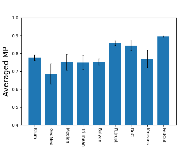
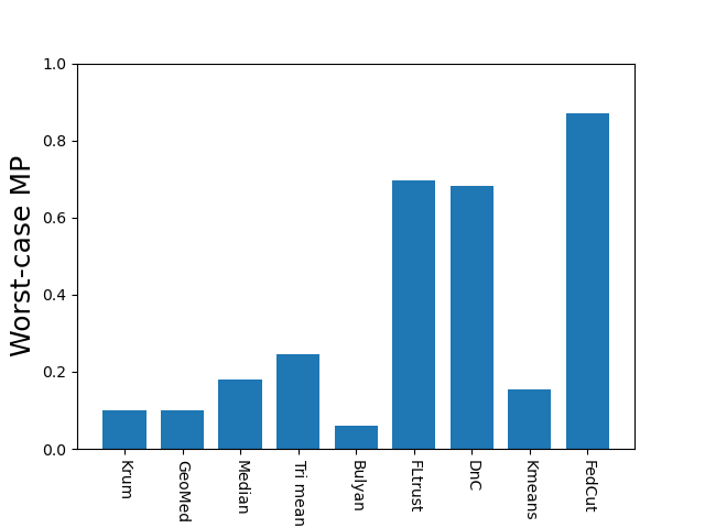
This paper proposes a general spectral analysis framework that thwarts a security risk in federated Learning caused by groups of malicious Byzantine attackers or colluders, who conspire to upload vicious model updates to severely debase global model performances. The proposed framework delineates the strong consistency and temporal coherence between Byzantine colluders’ model updates from a spectral analysis lens, and, formulates the detection of Byzantine misbehaviours as a community detection problem in weighted graphs. The modified normalized graph cut is then utilized to discern attackers from benign participants. Moreover, the Spectral heuristics is adopted to make the detection robust against various attacks. The proposed Byzantine colluder resilient method, i.e., FedCut, is guaranteed to converge with bounded errors. Extensive experimental results under a variety of settings justify the superiority of FedCut, which demonstrates extremely robust model performance (MP) under various attacks. It was shown that FedCut’s averaged MP is 2.1% to 16.5% better than that of the state of the art Byzantine-resilient methods. In terms of the worst-case model performance (MP), FedCut is 17.6% to 69.5% better than these methods.
Index Terms:
Byzantine colluders; Byzantine resilient; Spectral analysis; Normalized cut; Spectral heuristics; Graph; Federated learning; privacy preserving computing;1 Introduction
Federated learning (FL) [40, 66] is a suite of privacy-preserving machine learning techniques that allow multiple parties to collaboratively train a global model, yet, without gathering or exchanging privacy for the sake of compliance with private data protection regulation rules such as GDPR111GDPR is applicable as of May 25th, 2018 in all European member states to harmonize data privacy laws across Europe. https://gdpr.eu/. It is the upgraded global model performance that motivates multiple parties to join FL, however, the risk of potential malicious attacks aiming to degrade FL model performances cannot be discounted. It was shown that even a single attacker (aka a Byzantine worker) may prevent the convergence of a naive FL aggregation rule by submitting vicious model updates to outweigh benign workers (see Lemma 1 of [6]). A great deal of research effort was then devoted to developing numerous Byzantine-resilient methods which can effectively detect and attenuate such misbehaviours [6, 68, 45, 13, 61, 65, 21]. Nevertheless, recent research pointed out that a group of attackers or colluders may conspire to cause more damages than these Byzantine-resilient methods can deal with (see [4, 63, 18]). It is the misbehavior of such Byzantine colluders that motivate our research to analyze their influences on global model performances from a spectral analysis framework, and based on our findings, an effective defense algorithm to do away with Byzantine colluders is proposed.
There are two main challenges brought by Byzantine colluders. First, colluders may conspire to misbehave consistently and introduce statistical bias to break down Robust Statistics (RS) based resilient methods (e.g., [4, 18, 63]). Consequently, the global model performances may deteriorate significantly. Second, Byzantine colluders may conspire to violate the assumption that all malicious model updates form one group while benign ones form the other, which is invariably assumed by most clustering-based Byzantine-resilient methods [54, 51, 20]. By submitting multiple groups of such detrimental yet disguised model updates, colluders therefore can evade clustering-based methods and degrade the global model performance significantly.
In order to address the challenges brought by colluders, we propose in this article a spectral analysis framework, called FedCut, which admits effective detection of Byzantine colluders in a variety of settings and provide the spectral analysis of different types of Byzantine behaviours especially for Byzantine colluders (see Sect. 4). The essential ingredients of the proposed framework are as follows. First, we build the Spatial-Temporal graph with all clients’ model updates over multiple learning iterations as nodes, and similarities between respective pairs of model updates as edge weights (see Sect. 5.1). Second, an extension of the normalized cut (Ncut) [55, 42] provides the optimal c-partition Ncut (see Sect. 5.2), which allows to detect colluders with consistent behaviour efficiently. Third, spectral heuristics [70] are used to determine the type of Byzantine attackers, the unknown number of colluder groups and the appropriate scaling factor of Gaussian kernels used for measuring similarities between model updates (see Sect. 5.3). By leveraging the aforementioned techniques together within the unified spectral analysis framework, we thus propose in Sect. 5 the FedCut method which demonstrates superior robustness in the presence of different types of colluder attacks. Its convergence is theoretically proved in Sect. 6 and it compares favorably to the state of arts Byzantine-resilient methods in thorough empirical evaluations of model performances in Sect. 7. Our contributions are three folds.
-
•
First, we provide the spectral analysis of Byzantine attacks, especially, those launched by colluders. Specifically, we formulate existing Byzantine attacks as four types and gain a deeper understanding of colluders’ attacks in the lens of spectral. Moreover, we delineate root causes of failure cases of existing Byzantine-resilient methods in the face of colluder attacks (see Sect. 4.3).
-
•
Second, we propose the spectral analysis framework, called FedCut, which distinguishes benign clients from multiple groups of Byzantine colluders. Specifically, the normalized cut, temporal consistency and the spectral heuristics are adopted to address challenges brought by colluders. Moreover, we provide the theoretical analysis of convergence of the proposed algorithm FedCut.
-
•
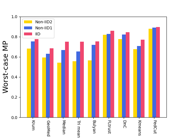
Finally, we propose to thoroughly investigate both averaged and worst-case model performances of different Byzantine-resilient methods with extensive experiments under a variety of settings, including different types of models, datasets, extents of Non-IID, the fraction of attackers, combinations of colluders groups. It was then demonstrated that the proposed FedCut consistently outperforms existing methods under all different settings (see Fig. 1 and Tab. I).
2 Related work
Related work are abundant in the literature and we briefly review them below.
Byzantine attacks can be broadly categorized as Non-Collusion and Collusion attacks. The former attacks were proposed to degrade global model performances by uploading Gaussian noise or flipping gradients [6, 35]. The latter type launched consistent attacks to induce misclassifications of Byzantine attackers [4, 18, 63].
Robust statistics based aggregation approaches treated malicious model updates as outliers, which are far away from benign clients, and filter out outliers via robust statistics accordingly. For example, the coordinate-wise Median and some variants of Median, such as geometric Median, were proposed to remove outliers [68, 45, 61]. Moreover, Blanchard et al. assumed few outliers were far away from benign updates. Therefore, they used the Krum function to select model updates that are very close to at least half the other updates [6] as benign updates.
However, the aforementioned methods are vulnerable to attacks with collusion which may conspire to induce biased estimations [4, 18, 63].
A different line of approaches [52, 16, 15] used the concentration filter to remove the outliers which are far away from concentration (such as the mean) [52, 16, 15]. For instance, Shejwalkar et al. applied SVD to the covariance matrix of model updates and filtered out outliers that largely deviate from the empirical mean of model updates towards the principle direction [52]. However, the effectiveness of the concentration filter may deteriorate in the presence of collusion attacks (see Sect. 4.3), and moreover, the time complexity of this approach is high when the dimension of updates is large.
Clustering based robust aggregation grouped all clients into two clusters according to pairwise similarities between clients’ updates and regarded the cluster with a smaller number as the Byzantine cluster. For instance, some methods applied Kmeans into clustering benign and byzantine clients [54, 9] and Sattler et al. separated benign and byzantine clients by minimizing cosine similarity of updates among two groups [51, 50]. Moreover, Ghosh et al. made use of iterative Kmeans clustering to remove the byzantine attackers [20].
However, the adopted naive clustering such as Kmeans,Kmedian [26, 38] have two shortcomings: 1) being inefficient and easily trapped into local minima; 2) breaking down when the number of colluder groups is unknown to the the clustering method (see details in Sect. 4).
Server based robust aggregation
assumed the server had an extra training dataset which was used to evaluate uploaded model updates. Either abnormal updates with low scores were filtered out [10, 62, 48, 46] or minority Byzantine updates were filtered out through majority votes [12, 47, 22].
However, this approach is not applicable to the case when the server-side data is not available, or it might break down if the distribution of server’s data deviates far from that of training data of clients.
Historical Information based byzantine robust methods made use of historical information (such as distributed Momentums [17]) to help correct the statistical bias brought by colluders during the training, and thus lead to the convergence of optimization of federated learning [3, 27, 2, 11, 29, 19].
Other byzantine robust methods used signs of the gradients [5, 56], optimization strategy [35] or sampling methods [28] to achieve robust aggregation. Recently, some work studied Byzantine-robust algorithms in the decentralized setting without server [21, 44, 24] and asynchronous setting with heterogeneous communication delays [14, 64, 67].
Community detection in graph. In the proposed framework, the detection of Byzantine colluders is treated as the detection of multiple subgraphs or communities in a large weighted graph (see Sect. 5.1). Existing approaches [41] could be applied to detect the byzantine colluders. One important technique is to detect specific features of graph such as clustering coefficients [59]. Another important technique is to leverage the spectral property of graph based on the adjacency matrix or normalized Laplacian matrix and so on [53, 49, 8].
Moreover, the number of communities can be determined based on the eigengap of these matrix [70] (see Sect. 5.3).
| Robust statistics based | Clustering based | Server based | Spectral based | |||||
| Krum | Median | Tri mean | DnC | Kmeans | FLtrust | FedCut(Ours) | ||
| Non-Collusion | Gaussian[6] | ✔ | ✔ | ✖ | ✖ | ✔ | ✔ | |
| label flipping[15] | ✖ | ✖ | ✔ | ✔ | ✔ | ✔ | ||
| sign flipping[15] | ✖ | ✖ | ✔ | |||||
| Collusion-diff | same value[35] | ✖ | ✖ | ✔ | ✔ | ✔ | ✔ | |
| Fang-v1[18] | ✖ | ✖ | ✔ | ✔ | ✔ | |||
| Multi-collusion | ✖ | ✖ | ✖ | ✔ | ✔ | |||
| Collusion-mimic | Mimic[28] | ✖ | ✔ | ✔ | ✔ | |||
| Lie [4] | ✖ | ✖ | ✖ | ✔ | ✖ | ✔ | ||
3 Preliminary
3.1 Federated Learning
We consider a horizontal federated learning [66, 40] setting consisting of one server and clients. We assume clients222In this article we use terms ”client”, ”node”, ”participant” and ”party” interchangeably. have their local dataset , where is the input data, is the label and is the total number of data points for client. The training in federated learning is divided into three steps which iteratively run until the learning converges:
-
•
The client takes empirical risk minimization as:
(1) where is the client’s local model weight and is a loss function that measures the accuracy of the prediction made by the model on each data point.
-
•
Each client sends respective local model updates to the server and the server updates the global model as , where is learning rate.
-
•
The server distributes the updated global model to all clients.
3.2 Byzantine Attack in Federated Learning
We assume a malicious threat mode where an unknown number of participants out of K clients are Byzantine, i.e., they may upload arbitrarily corrupt updates to degrade the global model performance (MP). Under this assumption, behaviours of Byzantine clients and the rest of benign clients can be summarized as follows:
| (2) |
Note that under the assumed threat mode, each adversarial node has access to updates of all clients during the training procedure. They are aware of the adoption of Federated Learning Byzantine-resilient methods [6, 4, 63], and conspire to upload specially designed model updates that may overwhelm existing defending methods. Byzantine clients who behave consistently as such are referred to as colluders throughout this article. Moreover, we assume the server to be honest and try to defend the Byzantine attacks.
4 Failure Cases Caused by Byzantine Colluders
The challenge brought by colluders is detrimental to Byzantine-resilient algorithms in different ways. We first analyze below behaviours of representative Byzantine attackers from a graph theoretic perspective. Then we demonstrate a toy example to showcase that existing Byzantine-resilient methods are vulnerable to collusion attacks.
4.1 Weighted Undirected Graph in Federated Learning
We regard model updates contributed by clients as an undirected graph , where represent model updates, is a set of weighted edge representing similarities between uploaded model updates corresponding to clients in . We assume that the graph is weighted, and each edge between two nodes and carries a non-negative weight, e.g., , where is uploaded gradient for client and is the Gaussian scaling factor. Let and respectively denote two subgraphs of representing benign and Byzantine clients.
Moreover, Byzantine problem [32] could be regarded as finding a optimal graph-cut for to distinguish the Byzantine and benign model updates. Since model updates from colluders form specific patterns (see Fig. 3 for examples), the aforementioned graph-cut can be generalized to the so called community-detection problem [41] in which multiple subsets of closely connected nodes are to be separated from each other.
4.2 Spectral Graph Analysis for Byzantine Attackers
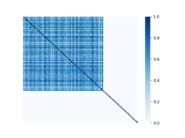
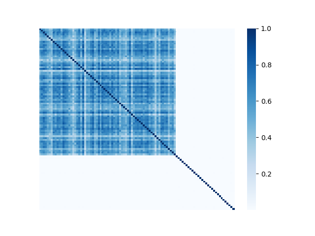
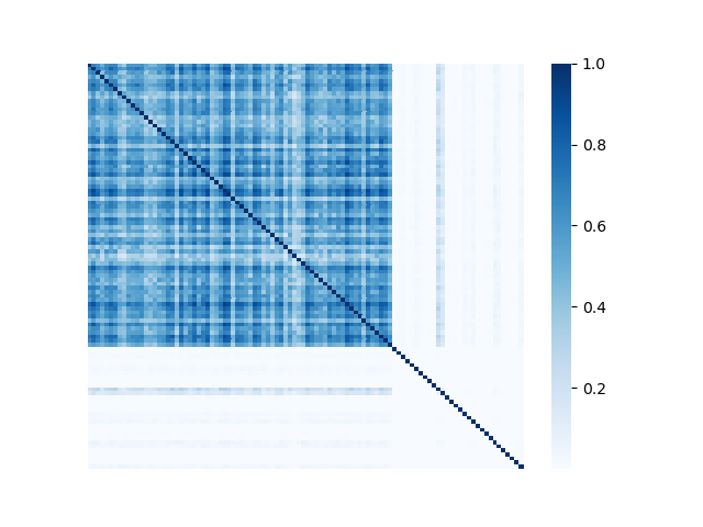
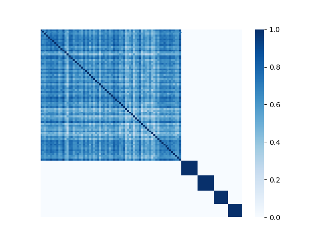
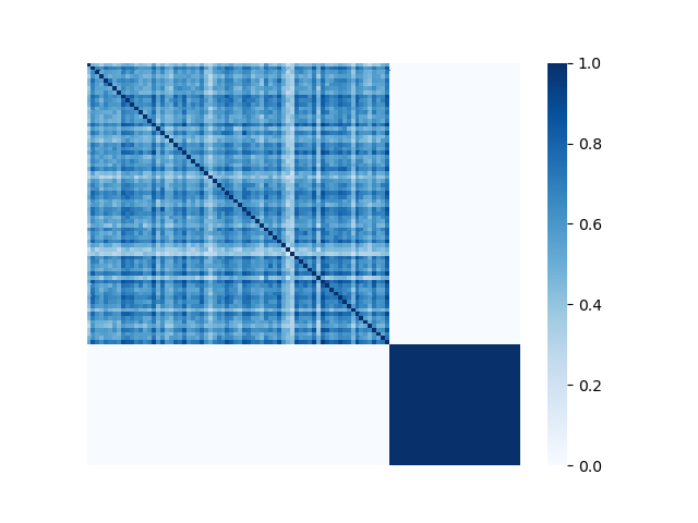
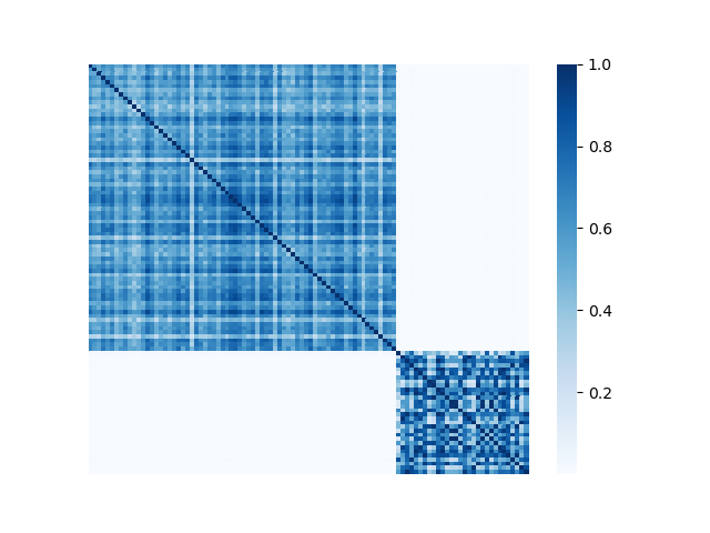
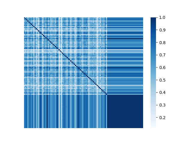
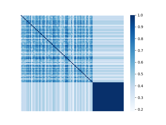
We illustrate the spectral analysis of representative Byzantine attacks, especially, those launched by colluders. For example, Fig. 2 shows adjacency matrices with elements representing pairwise similarities between 70 benign clients under IID setting and 30 attackers (the darker the element the higher the pairwise similarity is). It is clear in each subfigure that benign clients form a single coherent cluster residing in the upper-left block of the adjacent matrix333Note that the order of the nodes illustrated in Fig. 2 is irrelevant and we separate benign nodes from Byzantine nodes only for better visual illustration., while attackers reside in the bottom-right parts of the adjacent matrix. We observe the following characteristics pertaining to benign as well as Byzantine model updates.
First, benign model updates form a single group (upper-left block of Fig. 2), which is formally illustrated by Assumption 4.1, i.e., they all lie in the group (circle) with center and radius . Specifically, when the local datasets are homogeneous (IID), is small, indicating the strong similarity among benign model updates. When the local data of clients becomes heterogeneous, the radius becomes larger. Note that Assumption 4.1 has been widely used to bound differences between model updates of benign clients, e.g., in [37, 69].
Assumption 4.1.
Assume the difference of local gradients and the mean of benign model update is bounded ( is the set of benign clients), i.e., there exists a finite , such that
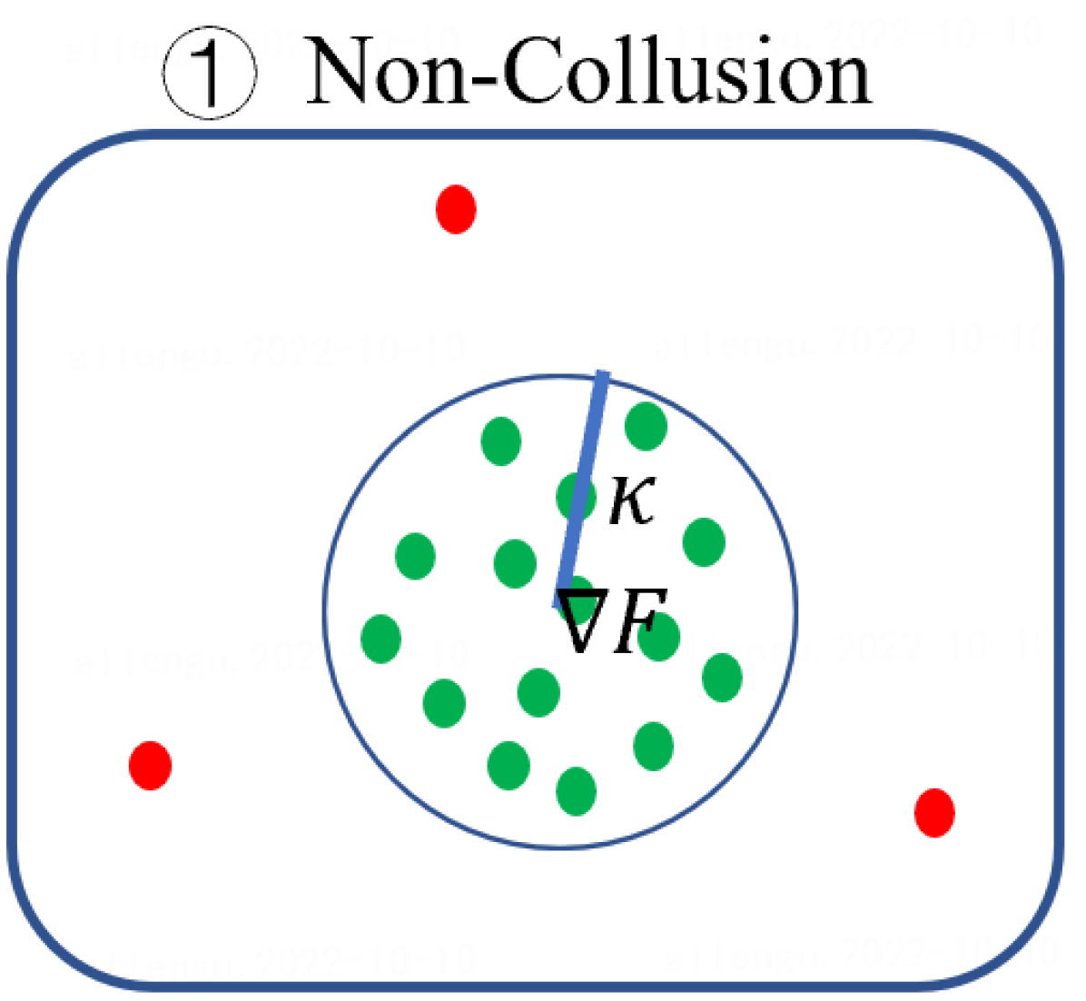
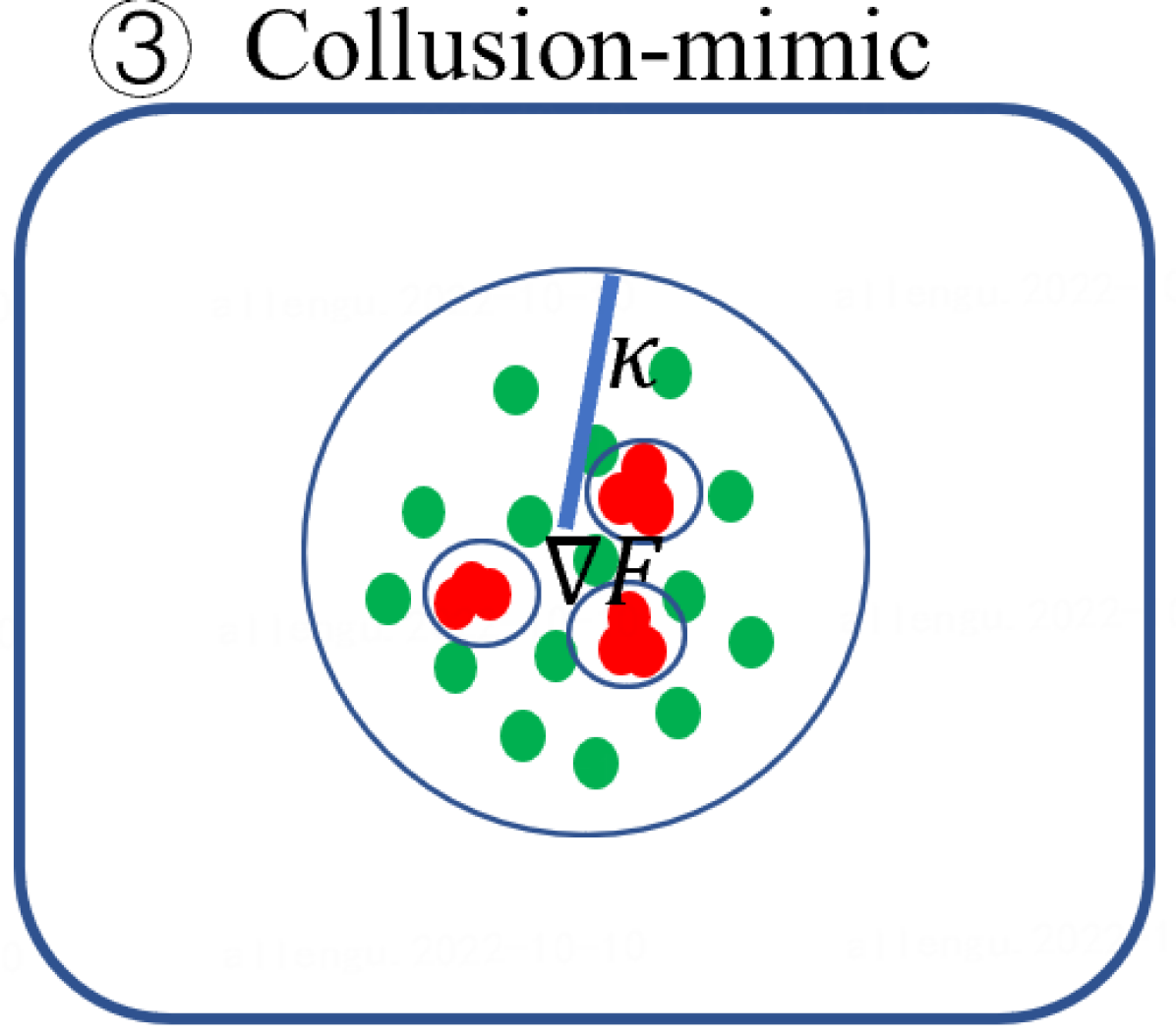
Second, Byzantine model updates can be categorized into four types (Fig. 3):
- •
- •
-
•
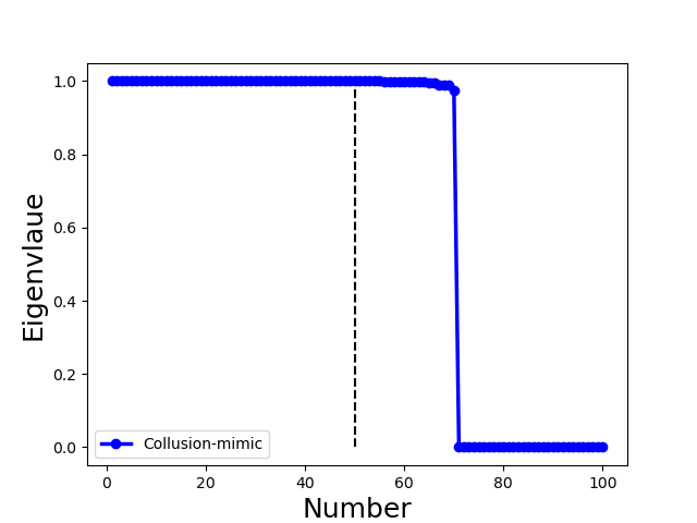
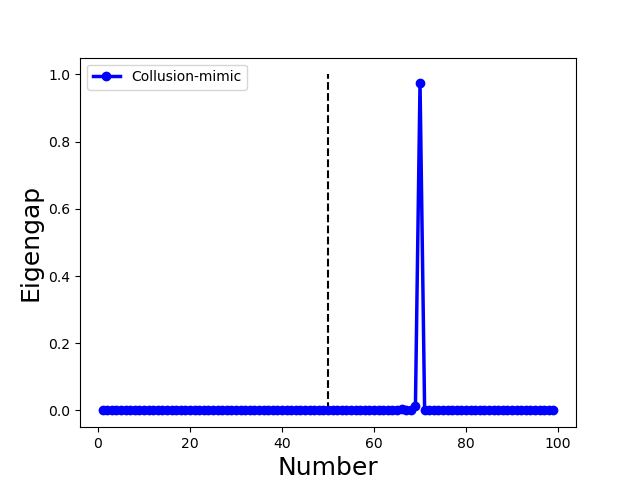
Collusion-mimic: and of different attackers are almost identical (). It represents adversaries with strong connections form one or multiple clusters (small intra-cluster distance), and their behaviours are very similar to the few selected benign clients but are different from the rest of benign clients (e.g., Mimic attack [28] and Lie [4] in Fig. 2(g) and (h)).
-
•
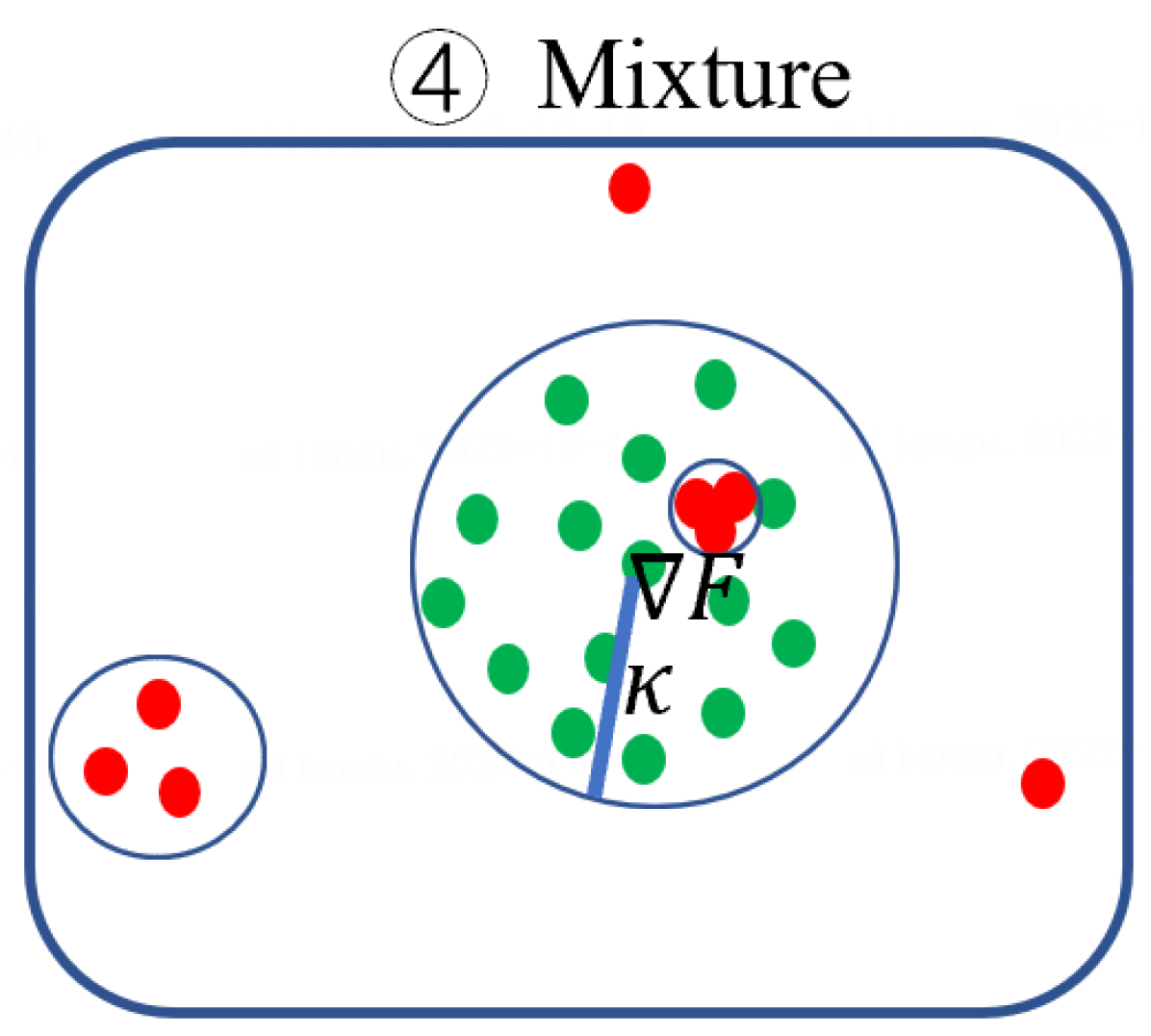
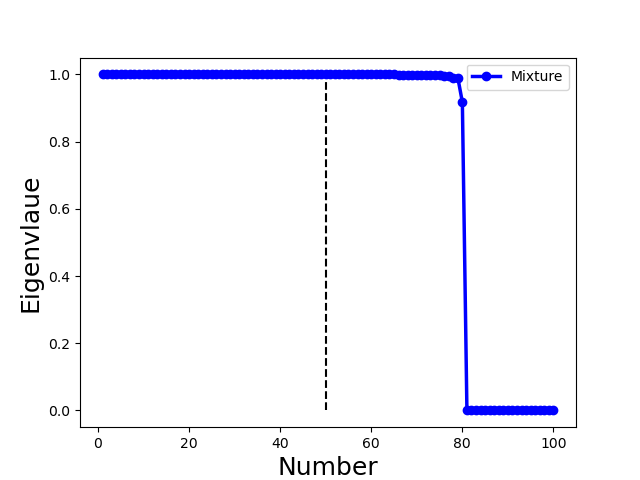
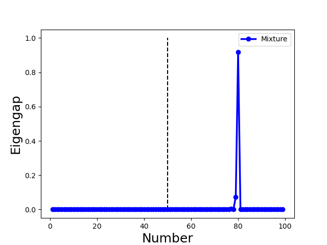
Mixture: adversaries may combine Non-collusion, Collusion-diff, and Collusion-mimic arbitrarily to obtain a mixture attack.
In order to address the complex types of both benign and Byzantine model updates, we adopt he eigengap technique [53, 70] to reliably detect benign and Byzantine clusters (or communities). We provide the following proposition to elucidate characteristics of different types of Byzantine attacks in the lens of spectral analysis. The proof of Proposition 4.1 is deferred to Appendix C.
Proposition 4.1.
Suppose clients consist of benign clients and attackers (). If Assumption 4.1 holds for Non-collusion and Collusion-diff attacks, then only the first eigenvalues are close to 1 and
-
•
for Non-collusion attacks provided that and malicious updates () are far away from each other;
-
•
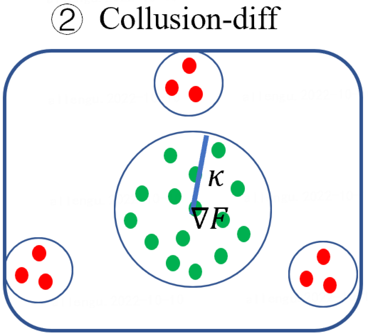
for Collusion-diff attacks provided that malicious updates form groups and ;
-
•
for Collusion-mimic attacks that and malicious updates are almost identical.
Remark 4.1.
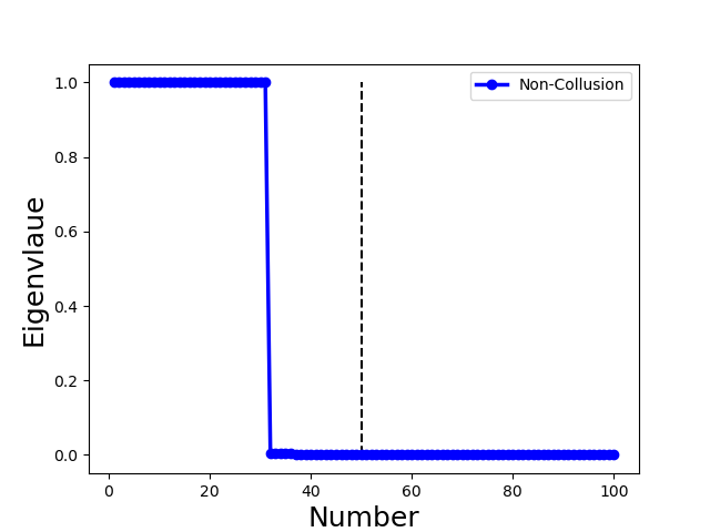
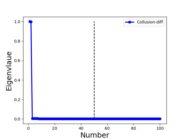
Proposition 4.1 illustrates that the eigenvalue 1 has multiplicity , and then there is a large gap to the eigenvalue . Therefore, we can use the position of the pronounced eigengap to elucidate the number of community clusters. Specifically, we use the largest eigengap to determine the number of the community clusters in our proposed method. Moreover, Proposition 4.1 demonstrates that the position of the pronounced eigengap for Non-collusion and Collusion-diff attacks is less than while larger than for Collusion-mimic attack. This property is used in the proposed method to distinguish Collusion-mimic attacks from other types of attacks (see Sect. 5.3.3).
We illustrate with a concrete example the different spectra of four types of attacks in Fig. 3, in which each column represents one type of attack. We observe the following properties (all of the examples include 70 benign clients and 30 attackers):
-
•
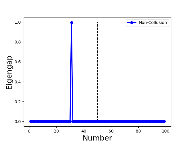
for Non-Collusion attack, we use the Gaussian attack [35] to upload largely different random updates following . Fig. 3(e) and (i) show the eigenvalue of adjacency matrix drops abruptly between index 30 and 31, i.e., the largest eigengap lies in index 31. It indicates the number of different communities is 31 with 70 benign clients forming a close group and 30 individual attackers forming other groups;
- •
-
•
for Collusion-mimic attack, we use the mimic attack [28] to upload updates that mimic one benign update, the largest eigengap is 70 because Byzantine colluders and mimiced benign clients form a group while the rest of 69 benign clients form 69 groups separately as Fig. 3(g) and (k) illustrate. It is because the connection among mimic colluders is much stronger than benign clients.
-
•
for Mixture attack, we combine the Gaussian attack (5 attackers), same-value attack (5 attackers), and mimic attack (20 attackers). Fig. 3(h) and (l) reveal that the largest eigengap is 80, in which mimic colluders and one mimiced benign client form a group. In contrast, 69 benign clients and 10 attackers form 79 groups separately. This example showcase that the mimic attack dominates the spectral characteristics of the Mixture attack. Therefore, for the proposed method, the Collusion-mimic type attack is first detected and removed, followed by the detection of other two types of attack (see Algo. 3 in Sect. 5.3.3 and line 3-4 of Algo. 2 in Sect. 5.2).
4.3 Failure Case Analysis
We evaluate two types of representative Byzantine-resilient methods (Robust statistics and the clustering based aggregation methods) and the proposed FedCut method (see Sect. 5.2) under four typical Byzantine Attacks mentioned in Sect. 4.2, in terms of their Byzantine Tolerance Rates (BTR) defined below. Specifically, we assume 10 benign model updates following 1D Gaussian distribution and see four types Byzantine attacks (S1-S4) as illustrated in Tab. II.
| Scenario | Attack Type | Attack Distribution | Number |
| S1 | Non-Collusion | 8 | |
| S2-s | Collusion-diff | 8 | |
| S2-m | Collusion-diff | 4 | |
| 4 | |||
| S3 | Collusion-mimic | 555 is the minimum elements of 10 benign model updates | 8 |
| S4 | Mixture | 3 | |
| 3 | |||
| 1 |
| BTR | Krum [6] | Median [68] | Trimmed Mean [68] | DnC [52] | Kmeans [54] | FedCut (ours) |
| S1 | 96.0% | 96.2% | 92.6% | 95.3% | 70.5% | 96.2% |
| S2-s | 34.5% | 29.5% | 27.5% | 89.6% | 99.0% | 99.0% |
| S2-m | 86.1% | 89.3% | 88.2% | 99.4% | 3.5% | 99.6% |
| S3 | 29.6% | 36.9% | 37.7% | 52.9% | 33.7% | 98.7% |
| S4 | 59.5% | 61.5% | 67.6% | 53.1% | 85.6% | 95.9% |
Next, we provide a toy example of four types of Byzantine attacks mentioned above to illustrate failure cases of existing Byzantine-resilient methods.
In order to evaluate different Byzantine-resilient methods under the four scenarios, we define the Byzantine Tolerant Rate representing the fraction of Byzantine Tolerant cases over repeated runs against attacks as follows:
Definition 4.1.
(Byzantine Tolerant Rate) Suppose the server receives correct gradients and Byzantine gradients . A Byzantine robust method is said to be Byzantine Tolerant to certain attacks [63] if
| (3) |
Moreover, the Byzantine Tolerant Rate (BTR) for is the fraction of Byzantine Tolerant cases over repeated runs against attacks.
Tab. III summarized toy example results for different Byzantine-resilient methods under four types of Byzantine attacks mentioned above. We can draw following conclusions:
-
•
First, for Non-Collusion attack (S1), all Byzantine-resilient methods except Kmeans [54] perform well (i.e., the BTR is higher than 90%), which indicates that Non-Collusion attack is easy to be defended.
-
•
Second, for Collusion-diff attack (S2), Robust Statistics based methods such as Krum [6], Median, Trimmed Mean [68] and DnC [52] are vulnerable to S2-s. This failure is mainly ascribed to the wrong estimation of sample mean or median misled by biased model updates from colluders. Moreover, the clustering based method i.e., Kmeans [54] fails in the S2-m, with BTR as low as 3.5%. This is because the clustering based method relies on the assumption that only one group of colluders exists, but two or more groups of colluders in S2-m are misclassified by naive clustering-based methods with wrong assumptions.
-
•
Third, for Collusion-mimic attack (S3), both Robust Statistics based methods and clustering based method fail, with BTR lower than 52.9%. The main reason is that colluders would introduce statistical bias for benign updates and similar behaviours of colluders are hard to detect.
-
•
Finally, the proposed FedCut method is able to defend against all attacks with high BTR (more than 95%) by using a Spatial-Temporal framework and spectral heuristics illustrated in Sect. 5.
It is worth mentioning that the toy example used in this Section only showcases some simplified failure cases that might defeat existing Byzantine-resilient methods. Instead, the attacking methods evaluated in Sect. 7 is more complex and detrimental, and we refer readers to thorough experimental results in Sect. 7 and Appendix B.
5 FedCut: Spectral Analysis against Byzantine Colluders
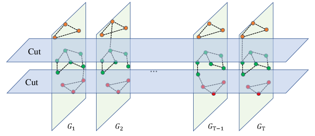
This section illustrates the proposed spectral analysis framework (see Algo. 1) in which distinguishing benign clients from one or more groups of Byzantine colluders is formulated as a community detection problem in Spatial-Temporal graphs [53], in which nodes represent all model updates and weighted edges represent similarities between respective pairs of model update over all training iterations (see Sect. 5.1). The normalized graph cut with temporal consistency [55, 42] (called FedCut) is adopted to ensure that a global optimal clustering is found (see Sect. 5.2). Moreover, the spectral heuristics [70] is then used to determine the Gaussian scaling factor, the number of colluder groups and the attack type (see Sect. 5.3). The gist of the proposed method is how to discern colluders from benign clients, by scrutinizing similarities between their respective model updates (see Fig. 4 for an overview).
5.1 A Spatial-Temporal Graph in Federated Learning
In order to use all information during the training, we define a Spatial-Temporal graph by considering behaviours of clients among all training iterations:
Definition 5.1.
(Spatial-Temporal Graph) Define a Spatial-Temporal graph as a sequence of snapshots , where is an undirected graph at iteration . denotes a fixed set of vertexes representing model updates belonging to clients. is a set of weighted edge representing similarities between model updates corresponding to clients in at iteration , where related adjacency matrix of the graph is .
Given a set of model updates from clients over iterations during federated learning, one is able to construct such a Spatial-Temporal graph by assigning edge weights as the measured pair-wise similarity between model updates.
The construction of the Spatial-Temporal graph with historical information is motivated by a common shortcoming of Byzantine-resilient methods, e.g., reported in [29], which showed that methods without using historical information during the training might lead to deteriorated global model performances in the presence of colluders. Our ablation study in Appendix B also confirmed the importance of using the Spatial-Temporal graph.
5.2 FedCut
As mentioned in Sect. 5.1, we have defined a Spatial-Temporal graph according to the model updates from clients over iterations during federated learning. Byzantine problem is then regarded as to find an optimal cut for such that the inter-cluster similarities (between benign clients and colluders) are as small as possible and intra-cluster similarities are as large as possible 666We view the cluster with the largest numbers as benign clients which constitute the largest community among all clients.. One optimal cut as such is known as the Normalized cut (Ncut) and has been initially applied to image segmentation [55, 42]. We adopt the Ncut approach to identify those colluders which have large intra-cluster similarities. Moreover, we extend the notion of Ncut to cater for the proposed Spatial-Temporal Graph over all iterations to make the detection of Byzantine colluders more consistent over multiple iterations. The c-partition Ncut for Spatial-Temporal Graph is thus defined as follows:
Definition 5.2.
(c-partition Ncut for Spatial-Temporal Graph) Let be a Spatial-Temporal graph as Def. 5.1. Denote the c-partition for graph as and for any , c-partition Ncut for Spatial-Temporal Graph aims to optimize:
| (4) |
where is the complement of , , and is edge weight of and , and .
The proposed FedCut (Algo. 2) is used to get rid of malicious updates before model updates are aggregated. FedCut computes adjacent matrix according to the uploaded gradients over all training iterations and then takes the normalized cut to distinguish benign clients and colluders. Specifically, three important parameters including the appropriate Gaussian kernel , the cluster number and the set of mimic colluders (who behave similarly to benign clients) need to be firstly determined (see Algo. 3). Then we calculate the adjacency matrix at iteration to remove the mimic colluders, i.e., set the connection between the mimic colluders and benign clients to be zero (line 2-7 in Algo. 2). We further compute normalized adjacency matrix by induction over iterations (line 8-9 in Algo. 2). Finally, we implement NCut into normalized adjacency matrix to choose the clusters of benign clients (line 10-12 in Algo. 2).
It is worth noting that FedCut runs over multiple learning iterations and, as shown by Proposition 5.1, it is guaranteed to provide the optimal c-partition Ncut defined by Eq. (4) (See Proof in Appendix C).
Proposition 5.1.
FedCut (Algo. 2) solves the c-partition Ncut for Spatial-Temporal Graph i.e., it obtains a optimal solution by:
.
5.3 Spectral Heuristics
The determination of three parameters (i.e., the scaling parameter of Gaussian kernels , the number of clusters and mimic colluders ) are critical in thwarting Byzantine Collusion attacks as illustrated in Sect. 4.3. We adopt the Spectral Heuristics about the following definition of eigengap to determine these three important parameters.
Definition 5.3.
The eigengap is defined as for which eigenvalues of the the normalized adjacency matrix are ranked in descending order, where . Let be the largest eigengap among .


5.3.1 Gaussian Kernel Determination
The Gaussian kernel scaling parameter in similarity function controls how rapidly the falls off with the distance between and . An appropriate is crucial for distinguishing Byzantine and benign clients. The following analysis shows that if the maximum eigengap (see Def. 5.3) is sufficiently large, a small perturbation on the normalized adjacency matrix or will only affect the eigenvectors with bounded influence, and thus the clustering of clusters via top eigenvectors are stable.
Proposition 5.2 (Stability [57]).
Let , and be eigenvalue, principle eigenvectors and the maximum eigengap of separately. Define a matrix small perturbation for as so that is small enough, let , be eigenvalue and principle eigenvectors of . If the maximum eigengap is large enough, then
| (5) |
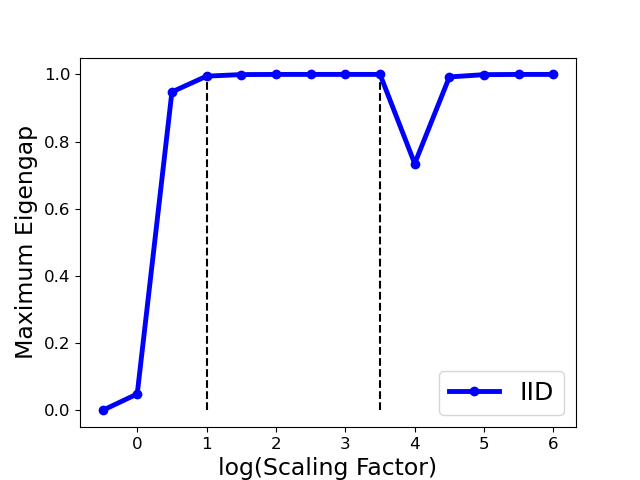
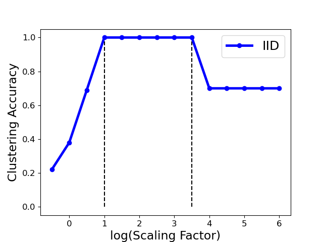
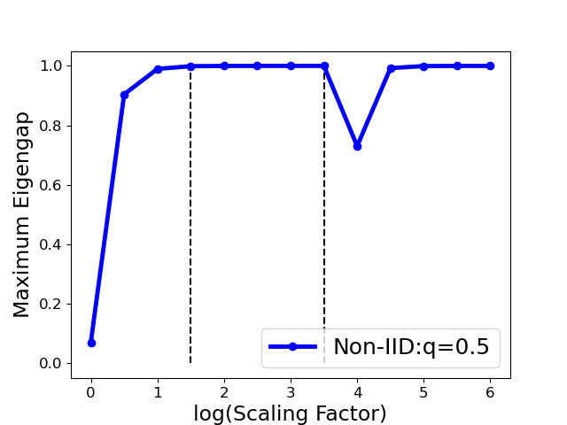
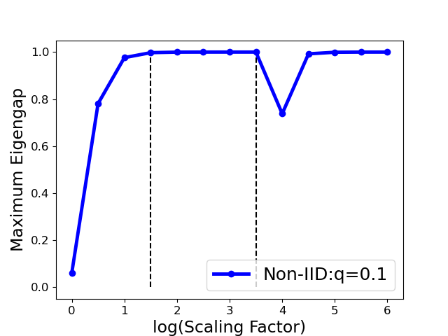
It is noted that the error bound in the principle eigenvectors is affected by two factors: the perturbation in the affinity matrix, and the maximal eigengap . While the perturbation is unknown and unable to modify for a given matrix , one can seek to maximize the eigengap so that the recovered principle eigenvectors are as stable as possible. According to proposition 5.2, we select the optimal parameter by maximizing the maximum eigengap, i.e.,
| (6) |
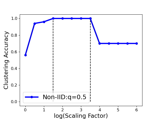
We implement this strategy in Algo. 3. Fig. 6 shows that one can select as such that the largest eigengap is up to its maximal (e.g., is in the range (1,3.5) for the Gaussian attack), provided that the clustering accuracy achieves the largest value (100%) in this range. Also noted that the clustering accuracy drops in the extreme case (i.e., the ) even the maximum eigengap is still large. Therefore, we select the optimal at one reasonable range with removing the extreme case (see detailed range in Sect. 7.1).
5.3.2 Determination of the Number of Clusters
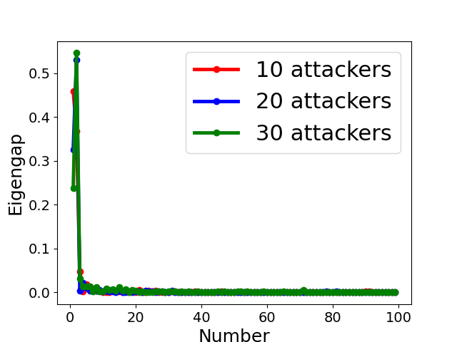
The assumption made by many clustering-based Byzantine-resilient methods that model updates uploaded by all Byzantine attackers form a single group might be violated in the presence of collusion (as shown by the toy example in Sect. 4.3 and experimental results in Sect. 7). Therefore, it is necessary to discover the number of clusters, and one possible way is to analyze the spectrum of the adjacency matrix, normalized adjacency matrix or correlation matrix [53]. According to the spectral property in Sect. 4.2, we determine the clustering number (see line 3-11 in Algo. 3) based on the position of the largest eigengap of normalized adjacency matrix, i.e.,
| (7) |
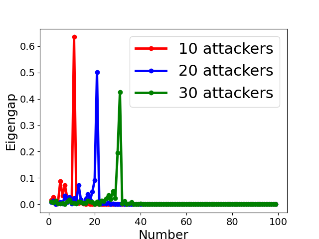
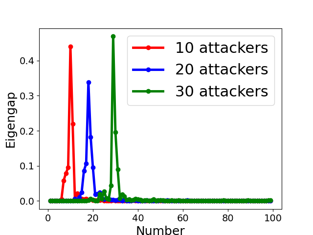
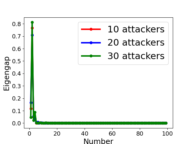
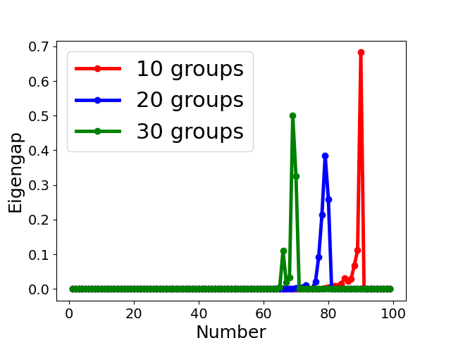
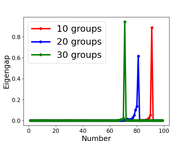
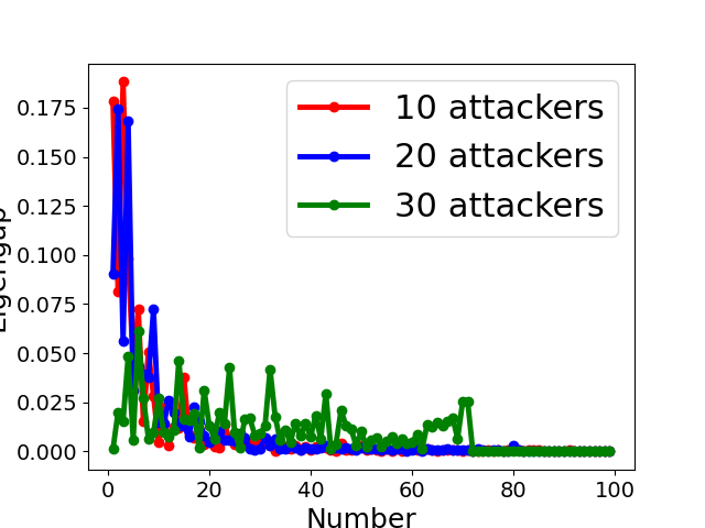
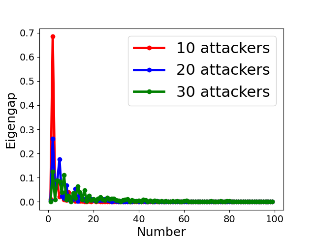
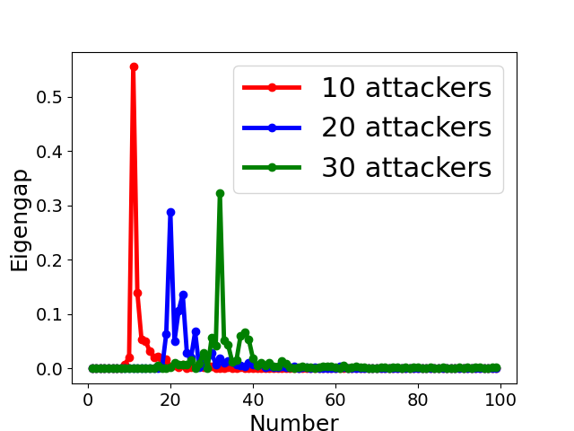
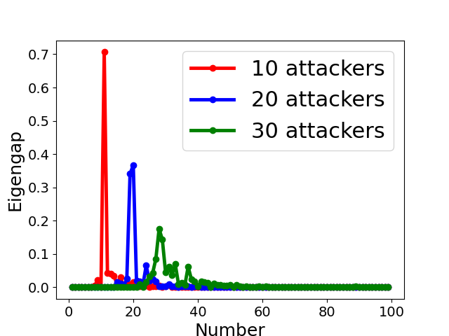
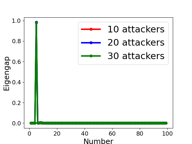
Fig. 5 displays the change of eigengap under different attacks, which shows that the index of the largest eigengap is a good estimation of the number of clusters. Specifically,
- •
-
•
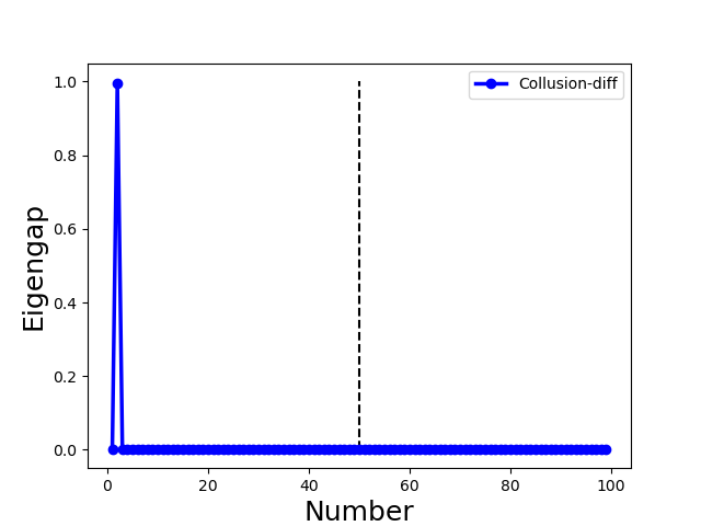
for Collusion-diff attack, the largest eigengap of Fig. 5(e) and (f) lies in between second and third largest eigenvalues. The position of the largest eigengap indicates that there are two clusters (one cluster represents benign clients while the other cluster represents colluders);
-
•
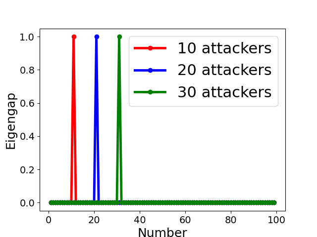
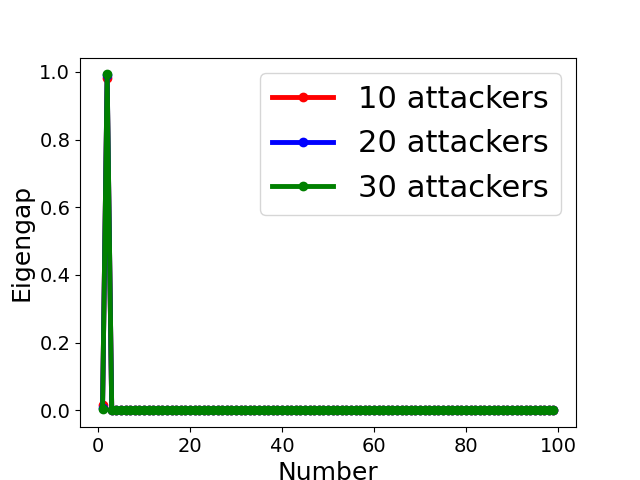
for Collusion-mimic attack, the largest eigengap in Fig. 5(a), (b), and (c) of 10, 20 and 30 attackers lies in 90, 80, and 70 indicating that cluster numbers are 90, 80, and 70 (colluders form one group while other benign clients form 90, 80, and 70 groups separately);
In addition, Our empirical results in Appendix B also demonstrates the effectiveness of estimating the number of communities via the largest eigengap even for heterogeneous dataset among clients.
5.3.3 Mimic Colluders Detection
Colluders may mimic the behaviours of some benign clients towards over-emphasizing some clients and render other model updates useless. Therefore, it is hard to distinguish the mimic colluders and benign clients. The existing byzantine-resilient methods could not defend the Collusion-mimic attack (see Sect. 4.3 for S3 case). We leverage the spectral property to detect the mimic colluders if the position of the largest eigengap is larger than (Proposition 4.1). Specifically, when the position of the largest eigengap is larger than , we pick the clusters with number of clients larger than two as mimic colluders sets (see line 12-15 in Algo. 3).
6 Convergence Analysis
We prove the convergence of such an iterative FedCut algorithm. The proof for Theorem 6.2 uses the similar technique as [15] (see details in Appendix C).
Assumption 6.1.
For malicious updates provided that , the difference between the mean of benign updates and colluders’ updates has at least distance, where is a large constant, i.e.,
Remark 6.1.
in the Assumption 6.1 is greatly larger than 1, which demonstrates a large distance between colluders and the mean of benign updates. If the single attacker uploads gradients within distance from the mean of benign updates, we can regard this attacker as one benign client. For mimic colluders who introduce the statistical bias, we detect these colluders and remove them according to spectral heuristics (see Sect. 5.3.3).
Theorem 6.1.
Remark 6.2.
The Theorem 6.1 illustrates that the distance between estimated gradients via FedCut and benign averaged gradients is bounded by . Moreover, is increasing w.r.t. when , and is increasing w.r.t. . Therefore, is increasing w.r.t. , which indicates that the probability decreases as the number of Byzantine attackers increases. In addition, for the larger , tends to zero since . Consequently, with a high probability close to 1.
Assumption 6.2.
The stochastic gradients sampled from any local dataset have uniformly bounded variance over for all benign clients, i.e., there exists a finite , such that for all , we have
| (8) |
where .
Remark 6.3.
Assumption 6.3.
We assume that F(x) is L-smooth and has -strong convex.
Theorem 6.2.
Suppose an fraction of clients are corrupted. For a global objective function , the server obtains a sequence of iterates (see Algo. 1) when run with a fixed step-size . If Assumption 4.1, 6.1, 6.2 and 6.3 holds, the sequence of average iterates satisfy the following convergence guarantees:
| (9) |
where , is a constant and is the global optimal weights in federated learning.
Theorem 6.2 provides the convergence guarantee of FedCut framework in the strong convex case. As tends to infinity, the upper bound of becomes large with the increasing of (variance of gradients within the same client), (variance between model updates across benign clients) and (the ratio of Byzantine attackers).
7 Experimental results
| Krum[6] | GeoMedian[13] | Median[68] | Trimmed[68] | Bulyan[21] | FLtrust[10] | DnC[52] | Kmeans[54] | FedCut(Ours) | ||
| M N I S T | No attack | 90.50.1 | 92.40.0 | 90.50.1 | 90.30.1 | 89.60.1 | 89.40.1 | 92.20.3 | 92.40.3 | 92.50.1 |
| Lie [4] | 90.50.0 | 84.40.6 | 84.00.3 | 83.60.8 | 73.61.0 | 89.50.1 | 92.20.3 | 92.20.2 | 92.30.2 | |
| Fang-v1 [18] | 90.20.1 | 45.80.5 | 43.41.5 | 37.82.6 | 85.50.3 | 75.83.5 | 92.30.3 | 92.30.2 | 92.30.1 | |
| Fang-v2 [18] | 41.17.4 | 53.42.1 | 39.02.3 | 42.42.8 | 18.86.1 | 79.70.8 | 92.00.6 | 88.20.4 | 92.30.1 | |
| Same value [35] | 90.60.1 | 85.60.0 | 77.00.4 | 75.10.6 | 88.80.4 | 89.80.3 | 92.30.2 | 92.20.3 | 92.20.1 | |
| Gaussian [6] | 90.40.1 | 92.40.1 | 90.60.1 | 90.80.1 | 89.60.3 | 87.01.0 | 74.30.4 | 22.44.3 | 92.30.1 | |
| sign flipping [15] | 90.60.1 | 91.30.1 | 90.20.1 | 90.20.1 | 89.60.2 | 72.25.5 | 90.70.1 | 49.91.3 | 91.90.2 | |
| label flipping [15] | 90.40.1 | 89.40.1 | 85.60.2 | 85.40.4 | 89.50.4 | 89.30.6 | 92.20.2 | 92.10.2 | 92.10.4 | |
| minic [28] | 86.10.4 | 86.30.9 | 88.30.3 | 89.70.2 | 85.50.5 | 90.50.1 | 92.20.4 | 92.10.1 | 92.30.1 | |
| Collusion (Ours) | 90.30.2 | 83.92.1 | 79.50.7 | 78.00.8 | 89.70.3 | 89.40.1 | 90.20.3 | 43.220.8 | 92.30.1 | |
| Averaged | 85.10.9 | 80.50.7 | 76.80.6 | 76.30.9 | 80.01.0 | 85.31.2 | 90.10.3 | 75.72.8 | 92.20.2 | |
| Worst-case | 41.17.4 | 45.80.5 | 39.02.3 | 37.82.6 | 18.86.1 | 72.25.5 | 74.30.4 | 22.44.3 | 91.90.2 | |
| F M N I S T | No attack | 84.60.5 | 89.50.3 | 88.20.4 | 88.60.4 | 87.30.3 | 88.20.5 | 90.30.2 | 90.00.3 | 90.10.3 |
| Lie [4] | 85.30.6 | 60.712.9 | 50.522.7 | 68.96.9 | 55.510.3 | 75.84.3 | 78.45.0 | 89.00.8 | 89.70.6 | |
| Fang-v1 [18] | 85.40.3 | 82.51.0 | 73.14.1 | 69.14.6 | 84.80.9 | 86.61.3 | 89.50.6 | 89.70.3 | 89.70.5 | |
| Fang-v2 [18] | 10.011.1 | 12.64.8 | 64.23.3 | 46.616.6 | 10.52.4 | 80.12.3 | 71.510.4 | 69.31.4 | 89.30.4 | |
| Same value [35] | 85.60.6 | 59.914.3 | 69.80.8 | 66.53.6 | 86.70.3 | 88.10.7 | 89.40.6 | 88.80.6 | 89.60.4 | |
| Gaussian [6] | 85.50.3 | 89.50.5 | 87.50.5 | 88.20.4 | 87.10.8 | 87.90.7 | 69.87.7 | 17.927.3 | 89.70.2 | |
| sign flipping [15] | 85.20.8 | 85.91.2 | 86.20.6 | 86.30.5 | 87.10.4 | 84.01.4 | 76.91.1 | 52.83.0 | 87.50.9 | |
| label flipping [15] | 85.50.2 | 89.60.3 | 72.65.1 | 78.54.8 | 87.10.3 | 87.90.6 | 89.80.3 | 89.90.4 | 89.10.3 | |
| minic [28] | 79.70.6 | 81.20.4 | 83.01.3 | 86.70.8 | 79.80.7 | 87.70.2 | 88.80.2 | 89.10.4 | 89.40.7 | |
| Collusion (Ours) | 84.70.5 | 35.922.7 | 71.26.3 | 69.51.8 | 86.80.6 | 88.40.3 | 85.51.7 | 76.913.6 | 90.00.5 | |
| Averaged | 77.21.6 | 68.75.8 | 74.64.5 | 74.94.0 | 75.31.7 | 85.51.2 | 83.02.8 | 75.34.8 | 89.40.5 | |
| Worst-case | 10.011.1 | 12.64.8 | 50.522.7 | 46.616.6 | 10.52.4 | 75.84.3 | 69.87.7 | 17.927.3 | 87.50.9 | |
| C I F A R 10 | No attack | 64.60.1 | 64.92.1 | 39.025.2 | 66.61.6 | 29.56.6 | 68.30.0 | 69.70.9 | 68.60.6 | 68.00.4 |
| Lie [4] | 63.92.1 | 10.00.2 | 10.20.2 | 9.80.2 | 10.00.1 | 12.44.2 | 11.93.3 | 20.422.0 | 68.40.4 | |
| Fang-v1 [18] | 64.40.5 | 63.90.3 | 11.22.1 | 17.512.3 | 17.33.4 | 68.10.8 | 66.80.3 | 68.00.9 | 67.73.9 | |
| Fang-v2 [18] | 9.90.1 | 15.04.1 | 11.01.3 | 11.31.4 | 10.00.1 | 61.84.2 | 67.00.6 | 53.412.7 | 68.51.5 | |
| Same value [35] | 64.80.7 | 50.20.3 | 10.00.0 | 10.00.0 | 54.80.2 | 29.233.3 | 65.15.2 | 65.311.3 | 66.41.8 | |
| Gaussian [6] | 63.51.1 | 62.14.3 | 48.44.8 | 65.40.2 | 17.16.2 | 68.10.6 | 31.82.3 | 12.61.3 | 65.30.7 | |
| sign flipping [15] | 65.00.5 | 58.612.5 | 16.65.6 | 51.91.7 | 40.214.9 | 28.732.4 | 47.59.4 | 17.722.6 | 63.15.5 | |
| label flipping [15] | 63.71.4 | 36.122.7 | 18.63.3 | 50.22.1 | 13.02.7 | 61.32.5 | 57.10.8 | 58.31.5 | 63.82.0 | |
| minic [28] | 44.10.9 | 65.00.5 | 56.41.0 | 66.00.8 | 42.22.8 | 48.032.9 | 65.91.7 | 66.63.6 | 68.80.2 | |
| Collusion (Ours) | 63.30.6 | 10.00.1 | 9.70.1 | 10.20.0 | 19.41.2 | 67.90.7 | 29.513.4 | 10.50.3 | 67.01.7 | |
| Averaged | 56.70.8 | 43.64.7 | 23.14.4 | 35.92.0 | 25.33.8 | 51.411.2 | 51.23.8 | 44.17.7 | 66.71.8 | |
| Worst-case | 9.90.1 | 10.00.2 | 9.70.1 | 9.80.2 | 10.00.1 | 12.44.2 | 11.93.3 | 10.50.3 | 63.15.5 |
This section illustrates the proposed FedCut method’s experimental results compared with eight existing Byzantine-robust methods. We refer to Appendix A and B for the full report of extensive experimental results.
7.1 Setup and Evaluation Metrics
- •
- •
-
•
Federated Learning Settings: We simulate a horizontal federated learning system with K = 100 clients in a stand-alone machine with 8 Tesla V100-SXM2 32 GB GPUs and 72 cores of Intel(R) Xeon(R) Gold 61xx CPUs. In each communication round, the clients update the weight updates, and the server adopts Fedavg [40] algorithm to aggregate the model updates. The detailed experimental hyper-parameters are listed in Appendix A.
-
•
Byzantine attacks: We set 10%, 20% and 30% clients, i.e., 10, 20, and 30 out of 100 clients are Byzantine attackers. The following attacking methods are used in experiments:
-
–
the same value attack: model updates of attackers are replaced by the all ones’ vector;
-
–
the sign flipping attack: local gradients of attackers are shifted by a scaled value -4;
-
–
the gaussian attack: local gradients at clients are replaced by independent Gaussian random vectors ;
-
–
the Lie attack: it was designed in [4];
- –
-
–
Mimic attack: Colluders may mimic the behaviours of some benign clients towards over-emphasizing some clients and under-representing others [28].
-
–
Our designed multi-collusion attack: adversaries are separated into 4 groups, and the same group has similar values. For example, each group is sampled from , and different groups have different , where is the mean of uploaded gradients of all other benign clients.
-
–
-
•
Byzantine-resilient methods: Nine existing methods i.e., Statistic-based methods: Krum [6], Median [68], Trimmed Mean [68], Bulyan [21] and DnC [52], Serve-evaluating methods: FLtrust [10], Clustering-based methods: Kmeans [54] and the proposed method FedCut are compared in terms of following metrics.
-
•
Gaussian kernel scaling parameters of FedCut: the preselected set of : in Algo. 3 is the geometric sequence with common ratio of for MNIST, for Fashion-MNIST and for CIFAR10.
Evaluation metric: two types of metrics are used in our evaluation.
-
•
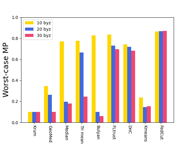
Model Performance (MP) of the federated model is used to evaluate defending capabilities of different methods. In order to elucidate robustness of each defending method, we also report respective averaged and worst-case model performances under all possible attacks.
-
•
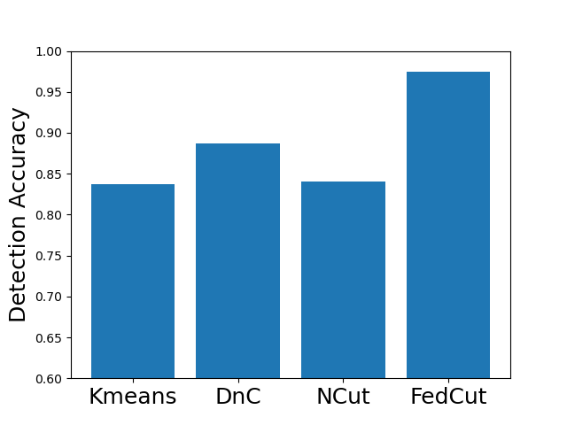
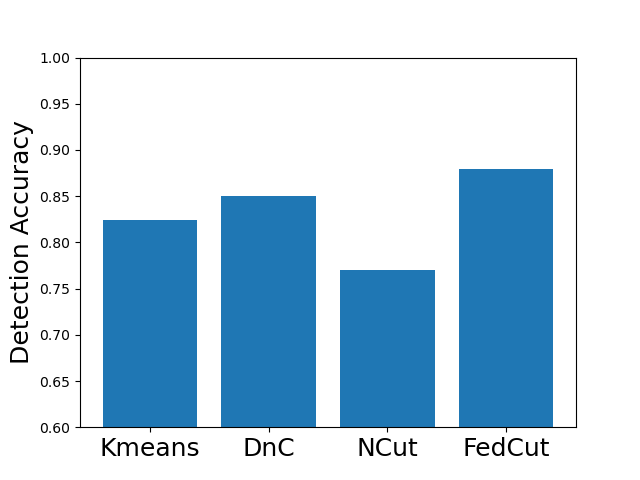
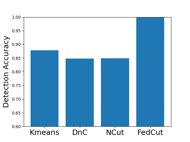
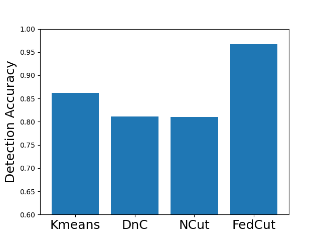
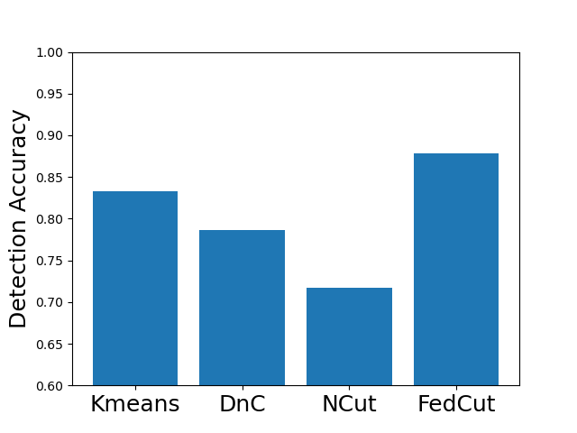
For methods including DnC [52], Kmeans [54] and FedCut, which detect benign clients before aggregation, detection accuracy among all iterations is used to quantify their defending capabilities. Note that this accuracy is measured against ground-truth Byzantine attackers’ membership, and it should not be confused with the image classification accuracy of the main task.
7.2 Comparison with Other Byzantine-resilient Methods
Tab. IV summarizes Model Performances (MP) of 8 existing methods as well as the proposed FedCut method for classification of MNIST, Fashion MNIST, and CIFAR10 using logistic regression, LeNet, and AlexNet respectively under IID setting and 30 attackers (see Appendix B for more results with other settings). There are four noticeable observations.
-
•
FedCut performs robustly under almost all attacks with worst-case MP above 92.0% for MNIST, 87.5% for Fashion MNIST and 63.1% for CIFAR10. This robust performance is in sharp contrast with eight existing methods, each of which has a worst-case MP degradation ranging from 18.2% (i.e., DnC by Gaussian attack reaching 74.3% MP) to 73.7% (i.e., Bulyan by Fang-v2 merely having 18.8% MP) on MNIST.
-
•
In terms of averaged MP, it is clearly observed that FedCut outperformed eight existing methods by noticeable margins ranging between 2.1% to 16.5% on MNIST, 3.9% to 20.7% on Fashion MNIST and 10.0% to 43.6% on CIFAR10.
-
•
Robust Statistics based methods (e.g., Krum, GeoMedian, Median, and Trimmed Mean) were overwhelmed by Collusion-diff and Collusion-mimic attacks (such as the MP drops 49.1% for Median under Fang-v1 attack and the MP drops 51.4% for Krum under Fang-v2 attack), incurred a significant MP degradation on MNIST. In contrast, all Collusion attacks cause a minor MP loss of less than 0.5% to FedCut.
-
•
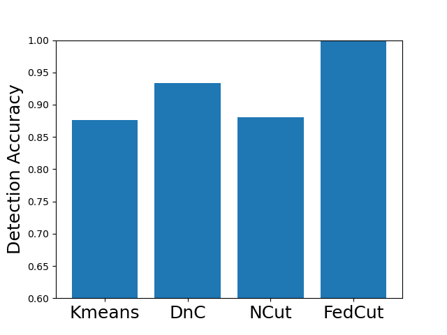
Existing clustering-based method, i.e., Kmeans performs robustly in the presence of single-group colluders but with MP degradation less than 2% (e.g., Kmeans for Same Value attack on MNIST, Fashion MNIST and CIFAR10), but incurred significant MP degradation more than 50% in the face of multi-group colluders attackers (e.g., Kmeans for the Multi-Collusion attack on MNIST and Gaussian attack on Fashion MNIST). In contrast, multi-group collusion doesn’t cause significant MP loss to the proposed FedCut, which adopts spectral heuristics to make an estimation of the number of colluder groups (see Sect. 5.3). Correspondingly, the detection accuracy of FedCut is higher than other methods, as Fig. 7 shows. For instance, the detection accuracy of FedCut on MNIST in the IID setting is 99.9%, while the detection accuracy of DnC and Kmeans drop to 93.6% and 87.5% separately.
7.3 Robustness
In this subsection, we demonstrate the robustness of our FedCut framework under different byzantine numbers, the Non-IID extent of clients’ local data, and multiple collusion attacks.
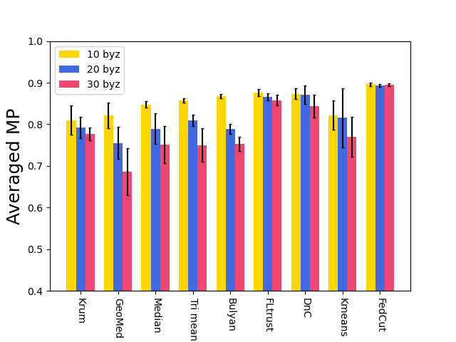
7.3.1 Robustness under Varying Numbers of Attackers.
Fig. 8 shows the model performance (MP) for different Byzantine-resilient methods under different types of attacks for different Byzantine attackers, i.e., 10, 20, and 30 attackers. The result shows that the MP of FedCut doesn’t drop with the increase of Byzantine numbers while the MP of others drops seriously (e.g., the averaged MP of Median [68] drops to 74.6% from 88.6% in Fashion MNIST dataset). Clearly, our proposed method, FedCut, is robust for the the number of byzantine attackers.
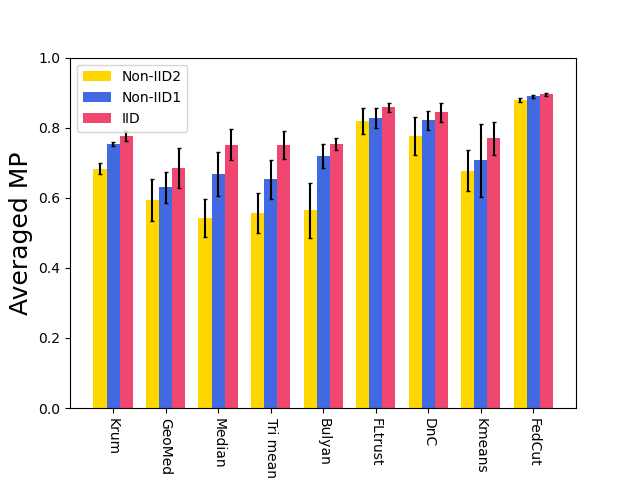
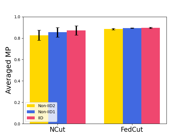
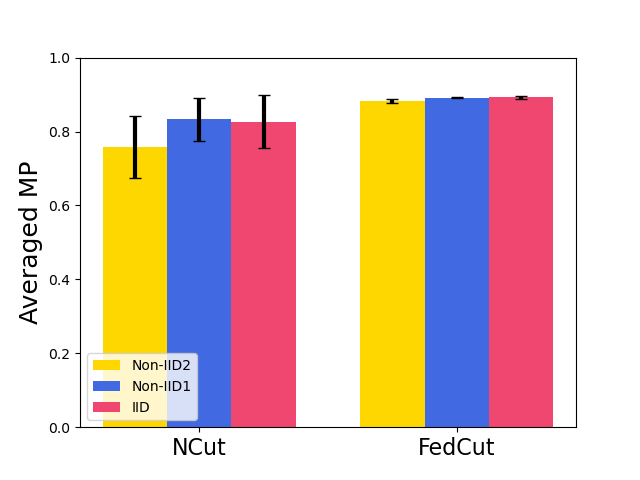
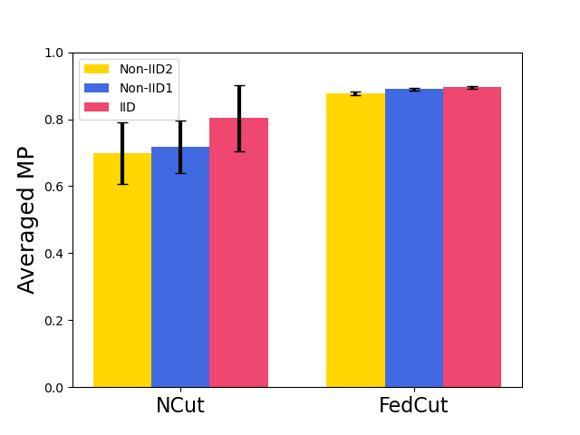
7.3.2 Robustness under Heterogeneous dataset
Fig. 9 shows the model performance (MP) for different Byzantine resilient methods under different types of attacks for different Non-IID extent of clients’ datasets. The result demonstrates that the MP of FedCut drops no more than 3% as the clients’ local dataset becomes more heterogeneous while the MP of others drops seriously (e.g., the averaged MP of trimmed mean [68] drops to 55.4% from 74.9% in Fashion MNIST dataset)
| Defense | Krum [6] | GeoMedian [13] | Median [68] | Trimmed [68] | Bulyan [21] | ||
|
|||||||
| Defense | FLtrust [10] | DnC [52] | Kmeans [54] | FedCut (Ours) | |||
|
7.3.3 Robustness against the Multi-Collusion attack
In the former part, we design the ’Multi-Collusion attack’ in which adversaries are separated into four groups, and the same group has similar values. For example, each group is sampled from , and different groups have different , where is the mean of uploaded gradients of all other benign clients. We further design more ’collusion attacks’ with a various number of colluders’ parties as follows: 30 attackers are separated into 1) two groups with each group having 15 attackers; 2) three groups with each group having ten attackers 3) four groups with each group having 8, 8, 7, 7 attackers respectively; 4) five groups with each group has six attackers.
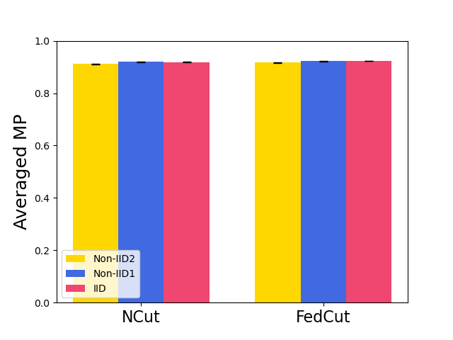
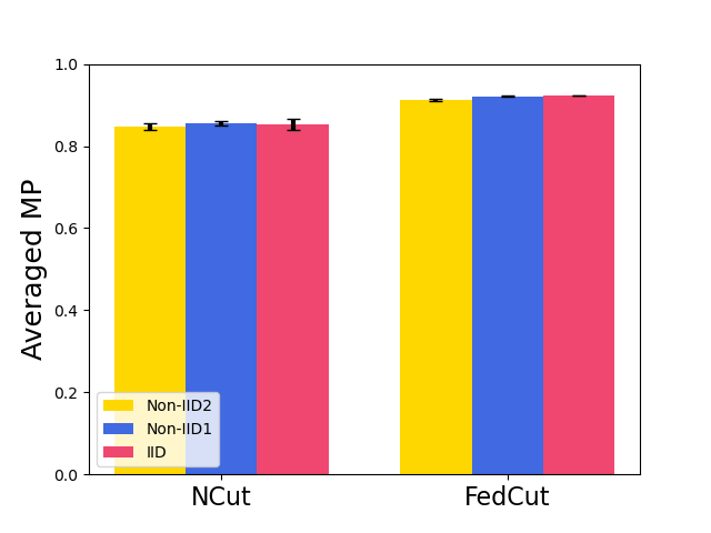
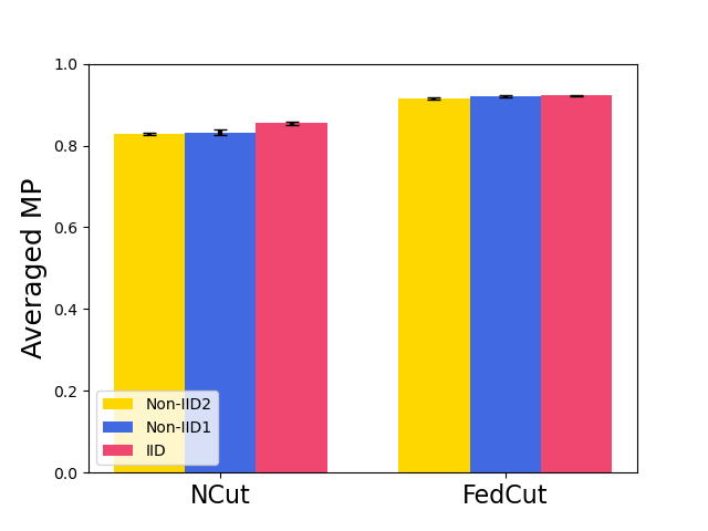
Tab. VII and VI displays the model performances under different ’collusion attacks,’ which illustrates that various collusion attacks do not influence FedCut and NCut while other byzantine resilient methods such as Kmeans are affected seriously by collusion attack. Note that DnC performs well with 2-groups collusion, but MP drops when colluders’ groups increase.
|
|
|
|
|
|
|
|
|
|||||||||||||||||||
| 2-groups | 89.20.4 | 79.20.0 | 71.90.1 | 69.00.2 | 89.10.2 | 88.50.1 | 91.90.1 | 45.70.0 | 91.70.0 | ||||||||||||||||||
| 3-groups | 88.90.1 | 81.10.0 | 73.40.0 | 70.70.1 | 88.90.1 | 88.00.1 | 87.20.8 | 45.90.1 | 91.60.1 | ||||||||||||||||||
| 4-groups | 89.00.5 | 82.21.2 | 73.61.2 | 72.31.2 | 86.71.2 | 89.20.5 | 89.40.5 | 31.22.2 | 92.10.1 | ||||||||||||||||||
| 5-groups | 88.81.1 | 84.20.1 | 78.00.1 | 75.10.0 | 88.70.1 | 88.40.1 | 89.00.3 | 54.10.0 | 91.70.1 |
|
|
|
|
|
|
|
|
|
|||||||||||||||||||
| 2-groups | 90.80.0 | 80.20.4 | 73.30.1 | 72.70.3 | 90.10.0 | 88.80.1 | 92.00.1 | 46.40.1 | 91.80.0 | ||||||||||||||||||
| 3-groups | 90.60.1 | 82.30.4 | 77.20.7 | 75.70.3 | 90.10.1 | 88.90.1 | 89.01.4 | 49.50.1 | 91.80.0 | ||||||||||||||||||
| 4-groups | 90.30.2 | 83.92.1 | 79.50.7 | 78.00.8 | 89.70.3 | 89.40.1 | 90.20.3 | 43.28.4 | 92.20.2 | ||||||||||||||||||
| 5-groups | 90.70.1 | 84.40.4 | 79.30.1 | 78.90.1 | 90.10.1 | 88.60.6 | 89.40.1 | 51.90.1 | 91.90.0 |
7.4 Computation Complexity
We compare the computation time complexity for different Byzantine resilient methods for each iteration on the server as Tab. V. It shows that the computation complexity of our proposed method FedCut is , where implementing the singular vector decomposition (SVD) needs [23] and computing the adjacency matrix requires . The time complexity of FedCut is comparable to statistic-based methods such as Krum [6] () and median [68] () when the dimension of model is greatly larger than number of participants .
Empirically, the proposed FedCut method allows the training of a DNN model (AlexNet) with 100 clients to run in three hours, under a simulated environment (see Appendix A for details). We regard this time complexity is reasonable for practical federated learning applications across multiple institutions. For cross-devices application scenarios in which might be up to millions, randomized SVD [23] can be adopted to improve the time complexity from to if the normalized adjacency matrix has low rank. Applying randomized SVD to cross-device FL scenarios is one of our future work.
8 Discussion and Conclusion
This paper proposed a novel spectral analysis framework, called FedCut, to detect Byzantine colluders robustly and efficiently from the graph perspective. Specifically, our proposed algorithm FedCut ensures the optimal separation of benign clients and colluders in the spatial-temporal graph constructed from uploaded model updates over different iterations. We analyze existing Byzantine attacks and Byzantine-resilient methods in the lens of spectral analysis. It was shown that existing Byzantine-resilient methods may suffer from failure cases in the face of Byzantine colluders. Moreover, spectral heuristics are used in FedCut to determine the number of colluder groups, the scaling factor and mimic colluders, which significantly improves the Byzantine tolerance in colluders detection.
Our extensive experiments on multiple datasets and theoretical convergence analysis demonstrate that our proposed framework can achieve drastic improvements over the FL baseline in terms of model performance under various Byzantine attacks.
Finally, the proposed and many existing Byzantine-resilient methods assume that the server could access to clients’ model updates to compute the similarity. However, the leakage of model updates allows a semi-honest server to infer some information of the private data [72]. Therefore, Byzantine problem should be considered when implementing FL for privacy-preserving applications. In future work, we will explore to what extent FedCut can be used in conjunction with Differential Privacy [1] or Homomorphic Encryption mechanisms [71].
References
- [1] Martin Abadi, Andy Chu, Ian Goodfellow, H Brendan McMahan, Ilya Mironov, Kunal Talwar, and Li Zhang. Deep learning with differential privacy. In Proceedings of the 2016 ACM SIGSAC conference on computer and communications security, pages 308–318, 2016.
- [2] Dan Alistarh, Zeyuan Allen-Zhu, and Jerry Li. Byzantine stochastic gradient descent. Advances in Neural Information Processing Systems, 31, 2018.
- [3] Zeyuan Allen-Zhu, Faeze Ebrahimianghazani, Jerry Li, and Dan Alistarh. Byzantine-resilient non-convex stochastic gradient descent. In International Conference on Learning Representations, 2020.
- [4] Gilad Baruch, Moran Baruch, and Yoav Goldberg. A little is enough: Circumventing defenses for distributed learning. Advances in Neural Information Processing Systems, 32, 2019.
- [5] Jeremy Bernstein, Jiawei Zhao, Kamyar Azizzadenesheli, and Anima Anandkumar. signsgd with majority vote is communication efficient and fault tolerant. In International Conference on Learning Representations, 2018.
- [6] Peva Blanchard, El Mahdi El Mhamdi, Rachid Guerraoui, and Julien Stainer. Machine learning with adversaries: Byzantine tolerant gradient descent. Advances in Neural Information Processing Systems, 30, 2017.
- [7] Stephen Boyd, Stephen P Boyd, and Lieven Vandenberghe. Convex optimization. Cambridge university press, 2004.
- [8] Andries E Brouwer and Willem H Haemers. Spectra of graphs. Springer Science & Business Media, 2011.
- [9] Saikiran Bulusu, Venkata Gandikota, Arya Mazumdar, Ankit Singh Rawat, and Pramod K Varshney. Byzantine resilient distributed clustering with redundant data assignment. In 2021 IEEE International Symposium on Information Theory (ISIT), pages 2143–2148. IEEE, 2021.
- [10] Xiaoyu Cao, Minghong Fang, Jia Liu, and Neil Zhenqiang Gong. Fltrust: Byzantine-robust federated learning via trust bootstrapping. arXiv preprint arXiv:2012.13995, 2020.
- [11] Chen Chen, Lingjuan Lyu, Yuchen Liu, Fangzhao Wu, Chaochao Chen, and Gang Chen. Byzantine-resilient federated learning via gradient memorization.
- [12] Lingjiao Chen, Hongyi Wang, Zachary Charles, and Dimitris Papailiopoulos. Draco: Byzantine-resilient distributed training via redundant gradients. In International Conference on Machine Learning, pages 903–912. PMLR, 2018.
- [13] Yudong Chen, Lili Su, and Jiaming Xu. Distributed statistical machine learning in adversarial settings: Byzantine gradient descent. Proceedings of the ACM on Measurement and Analysis of Computing Systems, 1(2):1–25, 2017.
- [14] Georgios Damaskinos, Rachid Guerraoui, Rhicheek Patra, Mahsa Taziki, et al. Asynchronous byzantine machine learning (the case of sgd). In International Conference on Machine Learning, pages 1145–1154. PMLR, 2018.
- [15] Deepesh Data and Suhas Diggavi. Byzantine-resilient high-dimensional sgd with local iterations on heterogeneous data. In International Conference on Machine Learning, pages 2478–2488. PMLR, 2021.
- [16] Ilias Diakonikolas, Gautam Kamath, Daniel Kane, Jerry Li, Ankur Moitra, and Alistair Stewart. Robust estimators in high-dimensions without the computational intractability. SIAM Journal on Computing, 48(2):742–864, 2019.
- [17] El Mahdi El Mhamdi, Rachid Guerraoui, and Sébastien Louis Alexandre Rouault. Distributed momentum for byzantine-resilient stochastic gradient descent. In 9th International Conference on Learning Representations (ICLR), number CONF, 2021.
- [18] Minghong Fang, Xiaoyu Cao, Jinyuan Jia, and Neil Gong. Local model poisoning attacks to Byzantine-Robust federated learning. In 29th USENIX Security Symposium (USENIX Security 20), pages 1605–1622, 2020.
- [19] Sadegh Farhadkhani, Rachid Guerraoui, Nirupam Gupta, Rafael Pinot, and John Stephan. Byzantine machine learning made easy by resilient averaging of momentums. arXiv preprint arXiv:2205.12173, 2022.
- [20] Avishek Ghosh, Justin Hong, Dong Yin, and Kannan Ramchandran. Robust federated learning in a heterogeneous environment. arXiv preprint arXiv:1906.06629, 2019.
- [21] Rachid Guerraoui, Sébastien Rouault, et al. The hidden vulnerability of distributed learning in byzantium. In International Conference on Machine Learning, pages 3521–3530. PMLR, 2018.
- [22] Nirupam Gupta, Thinh T Doan, and Nitin Vaidya. Byzantine fault-tolerance in federated local sgd under 2f-redundancy. arXiv preprint arXiv:2108.11769, 2021.
- [23] Nathan Halko, Per-Gunnar Martinsson, and Joel A Tropp. Finding structure with randomness: Probabilistic algorithms for constructing approximate matrix decompositions. SIAM review, 53(2):217–288, 2011.
- [24] Lie He, Sai Praneeth Karimireddy, and Martin Jaggi. Byzantine-robust decentralized learning via self-centered clipping. arXiv preprint arXiv:2202.01545, 2022.
- [25] Forrest N Iandola, Song Han, Matthew W Moskewicz, Khalid Ashraf, William J Dally, and Kurt Keutzer. Squeezenet: Alexnet-level accuracy with 50x fewer parameters and< 0.5 mb model size. arXiv preprint arXiv:1602.07360, 2016.
- [26] Anil K Jain and Richard C Dubes. Algorithms for clustering data. Prentice-Hall, Inc., 1988.
- [27] Peter Kairouz, H Brendan McMahan, Brendan Avent, Aurélien Bellet, Mehdi Bennis, Arjun Nitin Bhagoji, Kallista Bonawitz, Zachary Charles, Graham Cormode, Rachel Cummings, et al. Advances and open problems in federated learning. Foundations and Trends® in Machine Learning, 14(1–2):1–210, 2021.
- [28] Sai Praneeth Karimireddy, Lie He, and Martin Jaggi. Byzantine-robust learning on heterogeneous datasets via bucketing. arXiv preprint arXiv:2006.09365, 2020.
- [29] Sai Praneeth Karimireddy, Lie He, and Martin Jaggi. Learning from history for byzantine robust optimization. In International Conference on Machine Learning, pages 5311–5319. PMLR, 2021.
- [30] Alex Krizhevsky, Geoffrey Hinton, et al. Learning multiple layers of features from tiny images. 2009.
- [31] Alex Krizhevsky, Ilya Sutskever, and Geoffrey E Hinton. Imagenet classification with deep convolutional neural networks. Advances in neural information processing systems, 25, 2012.
- [32] Leslie Lamport, Robert Shostak, and Marshall Pease. The byzantine generals problem. In Concurrency: the Works of Leslie Lamport, pages 203–226. 2019.
- [33] Yann LeCun, Léon Bottou, Yoshua Bengio, and Patrick Haffner. Gradient-based learning applied to document recognition. Proceedings of the IEEE, 86(11):2278–2324, 1998.
- [34] Yann LeCun et al. Lenet-5, convolutional neural networks. URL: http://yann. lecun. com/exdb/lenet, 20(5):14, 2015.
- [35] Liping Li, Wei Xu, Tianyi Chen, Georgios B Giannakis, and Qing Ling. Rsa: Byzantine-robust stochastic aggregation methods for distributed learning from heterogeneous datasets. In Proceedings of the AAAI Conference on Artificial Intelligence, volume 33, pages 1544–1551, 2019.
- [36] Qinbin Li, Yiqun Diao, Quan Chen, and Bingsheng He. Federated learning on non-iid data silos: An experimental study. arXiv preprint arXiv:2102.02079, 2021.
- [37] Xiang Li, Wenhao Yang, Shusen Wang, and Zhihua Zhang. Communication efficient decentralized training with multiple local updates. arXiv preprint arXiv:1910.09126, 5, 2019.
- [38] Stuart Lloyd. Least squares quantization in pcm. IEEE transactions on information theory, 28(2):129–137, 1982.
- [39] Helmut Lutkepohl. Handbook of matrices. Computational statistics and Data analysis, 2(25):243, 1997.
- [40] Brendan McMahan, Eider Moore, Daniel Ramage, Seth Hampson, and Blaise Aguera y Arcas. Communication-efficient learning of deep networks from decentralized data. In Artificial intelligence and statistics, pages 1273–1282. PMLR, 2017.
- [41] Mark EJ Newman. Detecting community structure in networks. The European physical journal B, 38(2):321–330, 2004.
- [42] Andrew Ng, Michael Jordan, and Yair Weiss. On spectral clustering: Analysis and an algorithm. Advances in neural information processing systems, 14, 2001.
- [43] Rafail Ostrovsky, Yuval Rabani, Leonard J Schulman, and Chaitanya Swamy. The effectiveness of lloyd-type methods for the k-means problem. Journal of the ACM (JACM), 59(6):1–22, 2013.
- [44] Jie Peng and Qing Ling. Byzantine-robust decentralized stochastic optimization. In ICASSP 2020-2020 IEEE International Conference on Acoustics, Speech and Signal Processing (ICASSP), pages 5935–5939. IEEE, 2020.
- [45] Krishna Pillutla, Sham M Kakade, and Zaid Harchaoui. Robust aggregation for federated learning. arXiv preprint arXiv:1912.13445, 2019.
- [46] Saurav Prakash and Amir Salman Avestimehr. Mitigating byzantine attacks in federated learning. arXiv preprint arXiv:2010.07541, 2020.
- [47] Shashank Rajput, Hongyi Wang, Zachary Charles, and Dimitris Papailiopoulos. Detox: A redundancy-based framework for faster and more robust gradient aggregation. Advances in Neural Information Processing Systems, 32, 2019.
- [48] Jayanth Reddy Regatti, Hao Chen, and Abhishek Gupta. Bygars: Byzantine sgd with arbitrary number of attackers using reputation scores.
- [49] Camellia Sarkar and Sarika Jalan. Spectral properties of complex networks. Chaos: An Interdisciplinary Journal of Nonlinear Science, 28(10):102101, 2018.
- [50] Felix Sattler, Klaus-Robert Müller, and Wojciech Samek. Clustered federated learning: Model-agnostic distributed multitask optimization under privacy constraints. IEEE transactions on neural networks and learning systems, 32(8):3710–3722, 2020.
- [51] Felix Sattler, Klaus-Robert Müller, Thomas Wiegand, and Wojciech Samek. On the byzantine robustness of clustered federated learning. In ICASSP 2020-2020 IEEE International Conference on Acoustics, Speech and Signal Processing (ICASSP), pages 8861–8865. IEEE, 2020.
- [52] Virat Shejwalkar and Amir Houmansadr. Manipulating the byzantine: Optimizing model poisoning attacks and defenses for federated learning. In NDSS, 2021.
- [53] Hua-Wei Shen and Xue-Qi Cheng. Spectral methods for the detection of network community structure: a comparative analysis. Journal of Statistical Mechanics: Theory and Experiment, 2010(10):P10020, 2010.
- [54] Shiqi Shen, Shruti Tople, and Prateek Saxena. Auror: Defending against poisoning attacks in collaborative deep learning systems. In Proceedings of the 32nd Annual Conference on Computer Security Applications, pages 508–519, 2016.
- [55] Jianbo Shi and Jitendra Malik. Normalized cuts and image segmentation. IEEE Transactions on pattern analysis and machine intelligence, 22(8):888–905, 2000.
- [56] Jy-yong Sohn, Dong-Jun Han, Beongjun Choi, and Jaekyun Moon. Election coding for distributed learning: Protecting signsgd against byzantine attacks. Advances in Neural Information Processing Systems, 33:14615–14625, 2020.
- [57] Gilbert W Stewart. Matrix perturbation theory. 1990.
- [58] Ulrike Von Luxburg. A tutorial on spectral clustering. Statistics and computing, 17(4):395–416, 2007.
- [59] Duncan J Watts and Steven H Strogatz. Collective dynamics of ‘small-world’networks. nature, 393(6684):440–442, 1998.
- [60] Han Xiao, Kashif Rasul, and Roland Vollgraf. Fashion-mnist: a novel image dataset for benchmarking machine learning algorithms. arXiv preprint arXiv:1708.07747, 2017.
- [61] Cong Xie, Oluwasanmi Koyejo, and Indranil Gupta. Generalized byzantine-tolerant sgd. Journal of Environmental Sciences (China) English Ed, 2018.
- [62] Cong Xie, Oluwasanmi Koyejo, and Indranil Gupta. Zeno: Byzantine-suspicious stochastic gradient descent. arXiv preprint arXiv:1805.10032, 24, 2018.
- [63] Cong Xie, Oluwasanmi Koyejo, and Indranil Gupta. Fall of empires: Breaking byzantine-tolerant sgd by inner product manipulation. In Uncertainty in Artificial Intelligence, pages 261–270. PMLR, 2020.
- [64] Cong Xie, Sanmi Koyejo, and Indranil Gupta. Zeno++: Robust fully asynchronous sgd. In International Conference on Machine Learning, pages 10495–10503. PMLR, 2020.
- [65] Haibo Yang, Xin Zhang, Minghong Fang, and Jia Liu. Byzantine-resilient stochastic gradient descent for distributed learning: A lipschitz-inspired coordinate-wise median approach. In 2019 IEEE 58th Conference on Decision and Control (CDC), pages 5832–5837. IEEE, 2019.
- [66] Qiang Yang, Yang Liu, Tianjian Chen, and Yongxin Tong. Federated machine learning: Concept and applications. ACM Transactions on Intelligent Systems and Technology (TIST), 10(2):1–19, 2019.
- [67] Yi-Rui Yang and Wu-Jun Li. Basgd: Buffered asynchronous sgd for byzantine learning. In International Conference on Machine Learning, pages 11751–11761. PMLR, 2021.
- [68] Dong Yin, Yudong Chen, Ramchandran Kannan, and Peter Bartlett. Byzantine-robust distributed learning: Towards optimal statistical rates. In International Conference on Machine Learning, pages 5650–5659. PMLR, 2018.
- [69] Hao Yu, Rong Jin, and Sen Yang. On the linear speedup analysis of communication efficient momentum sgd for distributed non-convex optimization. In International Conference on Machine Learning, pages 7184–7193. PMLR, 2019.
- [70] Lihi Zelnik-Manor and Pietro Perona. Self-tuning spectral clustering. Advances in neural information processing systems, 17, 2004.
- [71] Chengliang Zhang, Suyi Li, Junzhe Xia, Wei Wang, Feng Yan, and Yang Liu. BatchCrypt: Efficient homomorphic encryption for Cross-Silo federated learning. In 2020 USENIX annual technical conference (USENIX ATC 20), pages 493–506, 2020.
- [72] Ligeng Zhu, Zhijian Liu, and Song Han. Deep leakage from gradients. Advances in neural information processing systems, 32, 2019.
Appendix A Experiment Setting
This section illustrates the experiment settings of the empirical study of the proposed FedCut framework in comparison with existing Byzantine resilient methods.
Model Architectures The architectures we investigated include the well-known Logistic regression, LeNet [34] and AlexNet [31].
Dataset We evaluate Federated learning model performances with classification tasks on standard MNIST, Fashion MNIST [60] and CIFAR10 dataset. The MNIST database of 10-class handwritten digits has a training set of 60,000 examples, and a test set of 10,000 examples. Fashion MNIST is fashion product of MNIST including 60,000 images and the test set has 10,000 images. The CIFAR-10 dataset consists of 60000 colour images in 10 classes, with 6000 images per class. Respectively, we conduct stand image classification tasks of MNIST, Fashion MNIST and CIFAR10 with logistic regression, LeNet and AlexNet. According to the way we split the dataset for clients in federated learning, the experiments are divided into IID setting and Non-IID setting. Specifically, We consider lable-skew Non-IID federated learning setting, where we assume each client’s training examples are drawn with class labels following a dirichlet distribution () [36], with which is the concentration parameter controlling the identicalness among users (we use & 0.5 in the following).
Federated Learning Settings We simulate a horizontal federated learning system with K = 100 clients in a stand-alone machine with 8 Tesla V100-SXM2 32 GB GPUs and 72 cores of Intel(R) Xeon(R) Gold 61xx CPUs. In each communication round, the clients update the weight updates, and the server adopts Fedavg [40] algorithm to aggregate the model updates. The detailed experimental hyper-parameters are listed in Tab. VIII.
| Hyper-parameter | Logistic Regression | LeNet | AlexNet |
| Activation function | ReLU | ReLU | ReLU |
| Optimization method | Adam | Adam | Adam |
| Learning rate | 0.0005 | 0.001 | 0.001 |
| Weight Decay | 0.001 | 0.002 | 0.001 |
| Batch size | 32 | 32 | 64 |
| Data Distribution | IID and Non-IID ( | IID and Non-IID ( | IID |
| Iterations | 2000 | 3000 | 3000 |
| Number of Clients | 100 | 100 | 30 |
| Numbers of Attackers | 10, 20, 30 | 10, 20, 30 | 6 |
Attack: We set 10%, 20% and 30% clients, i.e., 10, 20 and 30 out of 100 clients be Byzantine attackers. The following attacking methods are used in experiments:
-
1.
the ’same value attack’, where model updates of attackers are replaced by the all ones vector;
-
2.
the ’label flipping attack’, where attackers use the wrong label to generate the gradients to upload;
-
3.
the ’sign flipping attack’, where local gradients of attackers are shifted by a scaled value -4;
-
4.
the ’gaussian attack’, where local gradients at clients are replaced by independent Gaussian random vectors .
-
5.
the ‘Lie attack’, which was designed in [4];
- 6.
- 7.
-
8.
Our designed ’collusion attack’ that adversaries are separated into 4 groups and same group has the similar values. For example, each groups is sampled from and different groups has different , where is mean of uploaded gradients of all other benign clients.
Byzantine-resilient methods The following Byzantine resilent methods are evaluated in experiments:
-
1.
Krum [6], we adopt codes from https://github.com/vrt1shjwlkr/NDSS21-Model-Poisoning/tree/main/femnist
-
2.
Median [68], we adopt codes from https://github.com/Liepill/RSA-Byzantine
-
3.
Trimmed Mean [68], we adopt codes from https://github.com/vrt1shjwlkr/NDSS21-Model-Poisoning/tree/main/femnist
-
4.
Bulyan [21], we adopt codes from https://github.com/vrt1shjwlkr/NDSS21-Model-Poisoning/tree/main/femnist
-
5.
DnC [52], we adopt codes from https://github.com/vrt1shjwlkr/NDSS21-Model-Poisoning/tree/main/femnist
-
6.
FLtrust [10], we adopt codes from https://people.duke.edu/~zg70/code/fltrust.zip
-
7.
Kmeans [54], we adopt codes from https://scikit-learn.org/stable/modules/generated/sklearn.cluster.KMeans.html
-
8.
NCut [42], we adopt NCut in each iteration separately for ablation study.
-
9.
FedCut, the proposed FedCut method applied to the Spatial-Temporal network.
Appendix B Ablation Study
In this section, we report more experimental results on different extent Non-IID (e.g., =0.1 and =0.5), number of byzantine attackers (e.g., 10, 20 and 30), model (e.g., logistic regression, LeNet and AlexNet) and dataset (e.g., MNIST, Fashion MNIST and CIFAR10).
B.1 More Experimental Results
Tab. IX-XXVI show the model performance (MP) for different Byzantine resilient methods under different types of attacks in various settings. All results show that the proposed method FedCut achieve the best model performances compared to other byzantine resilient methods when the Non-IID extent increases from to 0.1 and byzantine attackers numbers increases from 10 to 30. As shown by the ablation study, the MP of NCut is is not as stable as that of the proposed FedCut (e.g., MP drops to 31.7 % with Non-IID setting and 30 attackers under Fang-v1 attack).


|
|
|
|
|
|
|
|
|
||||||||||||||||||||
| F M N I S T | No attack | 75.71.1 | 88.50.9 | 76.54.0 | 81.61.4 | 75.51.5 | 85.61.6 | 89.10.4 | 88.70.7 | 88.91.0 | ||||||||||||||||||
| Lie [4] | 73.80.7 | 78.91.7 | 40.028.6 | 47.422.8 | 72.15.0 | 83.02.9 | 75.33.8 | 81.10.9 | 88.70.8 | |||||||||||||||||||
| Fang-v1 [18] | 75.42.3 | 86.71.1 | 64.77.7 | 62.317.1 | 74.43.3 | 83.93.0 | 89.90.2 | 76.68.1 | 89.21.4 | |||||||||||||||||||
| Fang-v2 [18] | 10.00.0 | 43.45.7 | 68.83.6 | 59.513.0 | 56.811.3 | 84.90.7 | 88.41.9 | 88.80.4 | 88.90.1 | |||||||||||||||||||
| Same value [35] | 75.81.2 | 75.01.6 | 78.34.9 | 78.53.5 | 76.72.9 | 85.92.0 | 89.50.2 | 89.20.5 | 89.30.6 | |||||||||||||||||||
| Gaussian [6] | 77.20.8 | 88.20.7 | 78.230.8 | 74.87.9 | 64.815.5 | 86.30.9 | 80.44.2 | 40.624.2 | 89.60.4 | |||||||||||||||||||
| sign flipping [15] | 75.92.4 | 87.41.1 | 78.92.9 | 72.414.3 | 67.715.6 | 85.31.3 | 85.51.3 | 54.910.0 | 84.40.9 | |||||||||||||||||||
| label flipping [15] | 76.60.9 | 88.10.9 | 69.07.5 | 78.71.6 | 60.220.9 | 85.81.3 | 89.40.5 | 87.81.0 | 88.00.4 | |||||||||||||||||||
| minic [28] | 75.51.4 | 87.90.6 | 77.12.1 | 86.00.3 | 79.30.3 | 87.40.4 | 88.90.3 | 88.90.2 | 88.90.7 | |||||||||||||||||||
| Collusion (Ours) | 75.91.6 | 34.911.2 | 72.71.1 | 69.32.2 | 71.84.4 | 87.10.1 | 66.66.6 | 56.622.3 | 89.10.4 | |||||||||||||||||||
| Averaged | 69.21.2 | 75.92.6 | 70.49.3 | 71.18.4 | 69.98.1 | 85.51.4 | 84.31.9 | 75.36.8 | 88.50.7 | |||||||||||||||||||
| Worst-case | 10.00.0 | 34.911.2 | 40.028.6 | 47.422.8 | 56.811.3 | 83.02.9 | 66.66.6 | 40.624.2 | 84.40.9 |
|
|
|
|
|
|
|
|
|
||||||||||||||||||||
| F M N I S T | No attack | 83.20.6 | 89.90.3 | 84.50.9 | 84.31.9 | 83.62.3 | 87.40.9 | 90.00.4 | 89.60.5 | 90.00.4 | ||||||||||||||||||
| Lie [4] | 83.50.7 | 84.30.6 | 55.118.7 | 75.86.0 | 82.61.8 | 83.62.5 | 71.029.0 | 80.21.3 | 89.90.6 | |||||||||||||||||||
| Fang-v1 [18] | 83.70.4 | 89.10.4 | 79.83.4 | 79.73.5 | 84.11.8 | 85.31.6 | 90.20.3 | 89.61.5 | 89.60.3 | |||||||||||||||||||
| Fang-v2 [18] | 10.00.0 | 60.36.3 | 72.22.3 | 73.11.5 | 73.02.0 | 85.71.0 | 89.01.3 | 88.70.5 | 89.20.4 | |||||||||||||||||||
| Same value [35] | 83.50.3 | 76.30.5 | 84.20.6 | 83.41.4 | 83.81.3 | 87.10.5 | 89.80.2 | 89.90.2 | 90.00.5 | |||||||||||||||||||
| Gaussian [6] | 83.10.4 | 89.70.3 | 84.51.3 | 85.31.2 | 79.94.6 | 87.20.6 | 78.14.6 | 49.616.0 | 89.80.1 | |||||||||||||||||||
| sign flipping [15] | 83.70.7 | 88.90.7 | 82.83.8 | 84.61.8 | 80.82.7 | 86.71.5 | 88.20.5 | 71.710.6 | 86.40.6 | |||||||||||||||||||
| label flipping [15] | 83.60.8 | 89.50.4 | 81.13.4 | 83.43.4 | 81.12.5 | 87.50.6 | 90.00.2 | 89.60.2 | 89.80.3 | |||||||||||||||||||
| minic [28] | 83.60.5 | 89.40.1 | 81.56.3 | 88.40.6 | 85.10.8 | 88.70.6 | 89.40.1 | 89.70.2 | 89.20.3 | |||||||||||||||||||
| Collusion (Ours) | 84.30.6 | 27.824.8 | 75.21.9 | 75.51.4 | 81.92.8 | 88.70.6 | 84.20.7 | 54.512.6 | 90.10.1 | |||||||||||||||||||
| Averaged | 76.20.5 | 78.53.4 | 78.14.3 | 81.42.3 | 81.62.3 | 86.81.0 | 86.03.7 | 79.34.4 | 89.40.4 | |||||||||||||||||||
| Worst-case | 10.00.0 | 27.824.8 | 55.118.7 | 73.11.5 | 73.02.0 | 83.62.5 | 71.029.0 | 49.616.0 | 86.40.6 |
|
|
|
|
|
|
|
|
|
||||||||||||||||||||
| F M N I S T | No attack | 84.70.7 | 90.00.4 | 87.90.4 | 88.20.4 | 87.00.6 | 88.00.6 | 90.20.2 | 89.80.4 | 90.20.1 | ||||||||||||||||||
| Lie [4] | 85.10.3 | 66.822.2 | 81.92.2 | 82.70.9 | 85.10.5 | 85.21.1 | 80.03.8 | 78.63.2 | 90.00.4 | |||||||||||||||||||
| Fang-v1 [18] | 84.90.6 | 88.70.7 | 86.50.4 | 86.60.6 | 86.90.4 | 87.41.0 | 89.90.4 | 90.10.2 | 87.82.1 | |||||||||||||||||||
| Fang-v2 [18] | 47.731.0 | 78.21.8 | 78.00.3 | 84.70.8 | 84.81.0 | 84.30.8 | 89.60.9 | 89.30.2 | 90.30.4 | |||||||||||||||||||
| Same value [35] | 85.30.5 | 76.90.4 | 85.50.5 | 85.10.7 | 87.20.5 | 88.20.9 | 90.20.6 | 90.30.2 | 90.30.1 | |||||||||||||||||||
| Gaussian [6] | 85.10.9 | 90.00.4 | 87.80.5 | 88.10.4 | 87.50.4 | 88.30.8 | 76.35.2 | 30.226.5 | 90.30.2 | |||||||||||||||||||
| sign flipping [15] | 85.00.4 | 89.40.3 | 87.90.4 | 88.20.4 | 87.10.4 | 86.51.9 | 89.30.6 | 87.70.6 | 89.41.0 | |||||||||||||||||||
| label flipping [15] | 84.90.5 | 89.90.2 | 85.61.1 | 85.10.7 | 87.10.4 | 88.20.8 | 90.40.4 | 90.10.2 | 88.00.2 | |||||||||||||||||||
| minic [28] | 85.30.2 | 89.40.4 | 87.90.7 | 89.40.5 | 86.90.3 | 89.10.3 | 89.80.4 | 89.90.2 | 89.80.2 | |||||||||||||||||||
| Collusion (Ours) | 85.30.5 | 54.74.5 | 79.11.3 | 78.10.4 | 87.50.4 | 88.70.2 | 85.00.5 | 67.62.9 | 90.10.0 | |||||||||||||||||||
| Averaged | 81.33.6 | 81.43.1 | 84.80.8 | 85.60.6 | 86.70.5 | 87.40.8 | 87.11.3 | 80.43.5 | 89.60.5 | |||||||||||||||||||
| Worst-case | 47.731.0 | 54.74.5 | 78.00.3 | 78.10.4 | 84.81.0 | 84.30.8 | 76.35.2 | 30.226.5 | 87.82.1 |
|
|
|
|
|
|
|
|
|
||||||||||||||||||||
| F M N I S T | No attack | 72.02.5 | 88.40.7 | 70.111.0 | 81.80.3 | 81.80.4 | 86.11.1 | 88.90.8 | 88.70.6 | 89.40.4 | ||||||||||||||||||
| Lie [4] | 75.41.2 | 64.49.9 | 35.525.0 | 41.319.5 | 26.928.5 | 76.84.0 | 72.16.8 | 88.10.6 | 88.12.3 | |||||||||||||||||||
| Fang-v1 [18] | 76.41.5 | 78.50.8 | 27.910.9 | 35.89.2 | 71.65.5 | 84.12.9 | 88.70.8 | 89.70.4 | 89.20.1 | |||||||||||||||||||
| Fang-v2 [18] | 10.00.0 | 10.91.2 | 18.818.4 | 32.95.8 | 23.69.0 | 84.90.4 | 82.28.1 | 65.810.3 | 89.00.3 | |||||||||||||||||||
| Same value [35] | 76.61.9 | 64.58.9 | 57.811.9 | 66.73.7 | 81.20.7 | 86.11.0 | 89.50.4 | 89.50.4 | 89.40.2 | |||||||||||||||||||
| Gaussian [6] | 76.40.4 | 88.00.7 | 76.42.7 | 79.41.4 | 78.23.5 | 85.71.9 | 76.46.6 | 20.728.9 | 89.30.1 | |||||||||||||||||||
| sign flipping [15] | 75.51.2 | 85.35.5 | 73.05.9 | 54.525.3 | 80.58.5 | 83.42.5 | 76.71.2 | 61.13.4 | 82.90.5 | |||||||||||||||||||
| label flipping [15] | 76.50.7 | 88.31.0 | 66.813.1 | 75.52.9 | 77.310.4 | 85.61.2 | 87.32.0 | 87.01.2 | 88.50.5 | |||||||||||||||||||
| minic [28] | 75.31.4 | 84.61.4 | 60.413.3 | 81.13.6 | 66.94.7 | 87.40.5 | 88.00.1 | 88.70.4 | 89.10.2 | |||||||||||||||||||
| Collusion (Ours) | 75.01.6 | 55.911.4 | 67.72.0 | 70.70.4 | 71.72.2 | 86.40.5 | 86.10.4 | 32.420.0 | 89.40.4 | |||||||||||||||||||
| Averaged | 68.91.2 | 70.94.2 | 55.411.4 | 62.07.2 | 66.07.3 | 84.71.6 | 83.62.7 | 71.26.6 | 88.40.5 | |||||||||||||||||||
| Worst-case | 10.00.0 | 10.91.2 | 18.818.4 | 32.95.8 | 23.69.0 | 76.84.0 | 72.16.8 | 20.728.9 | 82.90.5 |
|
|
|
|
|
|
|
|
|
||||||||||||||||||||
| F M N I S T | No attack | 82.30.7 | 90.00.3 | 85.61.0 | 86.50.4 | 85.52.8 | 88.10.6 | 89.41.0 | 88.41.0 | 90.20.2 | ||||||||||||||||||
| Lie [4] | 83.51.0 | 53.713.5 | 36.115.6 | 51.926.7 | 54.512.9 | 76.36.0 | 73.37.8 | 87.91.0 | 89.90.1 | |||||||||||||||||||
| Fang-v1 [18] | 84.80.7 | 85.51.1 | 75.52.5 | 71.87.3 | 83.10.9 | 84.41.4 | 89.21.3 | 88.81.2 | 89.40.2 | |||||||||||||||||||
| Fang-v2 [18] | 10.08.3 | 18.97.1 | 62.45.1 | 55.82.8 | 59.35.4 | 84.90.8 | 83.08.3 | 72.45.2 | 89.50.2 | |||||||||||||||||||
| Same value [35] | 83.70.8 | 64.88.2 | 77.72.7 | 71.55.5 | 86.21.0 | 86.90.7 | 88.81.2 | 89.01.2 | 89.40.1 | |||||||||||||||||||
| Gaussian [6] | 82.90.4 | 89.60.5 | 84.62.5 | 86.21.1 | 85.70.7 | 88.40.4 | 77.57.2 | 38.234.5 | 89.50.3 | |||||||||||||||||||
| sign flipping [15] | 82.91.4 | 87.70.9 | 85.01.0 | 85.00.9 | 85.11.4 | 84.41.8 | 85.01.5 | 74.37.4 | 86.00.1 | |||||||||||||||||||
| label flipping [15] | 82.41.1 | 89.90.4 | 79.43.4 | 80.41.8 | 80.36.6 | 88.10.2 | 88.41.2 | 88.61.5 | 89.30.3 | |||||||||||||||||||
| minic [28] | 81.12.6 | 87.51.1 | 83.00.4 | 87.80.3 | 76.31.5 | 88.70.3 | 89.30.3 | 89.40.3 | 88.90.6 | |||||||||||||||||||
| Collusion (Ours) | 84.51.0 | 41.717.0 | 72.01.2 | 61.415.3 | 81.45.0 | 88.70.7 | 86.90.5 | 56.59.7 | 89.90.3 | |||||||||||||||||||
| Averaged | 75.81.8 | 70.95.0 | 74.13.5 | 73.86.2 | 77.73.8 | 85.91.3 | 85.13.0 | 77.46.3 | 89.20.2 | |||||||||||||||||||
| Worst-case | 10.08.3 | 18.97.1 | 36.115.6 | 51.926.7 | 54.512.9 | 76.36.0 | 73.37.8 | 38.234.5 | 86.00.1 |
|
|
|
|
|
|
|
|
|
||||||||||||||||||||
| F M N I S T | No attack | 84.60.6 | 90.10.4 | 88.30.2 | 88.00.6 | 87.50.2 | 88.30.6 | 89.31.0 | 89.20.7 | 89.10.9 | ||||||||||||||||||
| Lie [4] | 84.70.7 | 76.318.9 | 69.026.6 | 75.23.1 | 82.40.2 | 79.04.2 | 79.74.6 | 89.01.0 | 88.81.0 | |||||||||||||||||||
| Fang-v1 [18] | 85.30.4 | 86.40.7 | 80.81.4 | 80.32.0 | 87.50.3 | 86.60.9 | 88.51.0 | 89.20.6 | 89.70.2 | |||||||||||||||||||
| Fang-v2 [18] | 38.021.1 | 46.49.7 | 70.91.4 | 71.02.1 | 17.212.5 | 82.90.8 | 85.06.4 | 86.62.3 | 90.00.2 | |||||||||||||||||||
| Same value [35] | 85.00.5 | 74.02.2 | 78.92.0 | 77.81.2 | 87.10.4 | 88.40.4 | 89.30.8 | 89.20.7 | 89.50.2 | |||||||||||||||||||
| Gaussian [6] | 85.20.5 | 89.90.4 | 88.10.3 | 88.50.3 | 87.10.4 | 88.10.5 | 78.66.6 | 40.733.8 | 89.40.2 | |||||||||||||||||||
| sign flipping [15] | 84.50.5 | 88.50.1 | 87.40.3 | 87.40.5 | 87.40.2 | 86.40.6 | 87.30.8 | 75.76.8 | 87.30.5 | |||||||||||||||||||
| label flipping [15] | 85.50.6 | 89.90.6 | 82.30.8 | 82.00.5 | 87.30.2 | 87.30.9 | 89.21.1 | 89.80.7 | 89.70.1 | |||||||||||||||||||
| minic [28] | 81.80.8 | 86.30.8 | 86.40.3 | 88.50.2 | 80.00.4 | 88.40.3 | 89.10.2 | 89.20.9 | 89.80.4 | |||||||||||||||||||
| Collusion (Ours) | 84.90.7 | 35.75.0 | 76.71.1 | 69.72.9 | 87.40.2 | 88.60.2 | 86.90.4 | 66.722.7 | 89.61.0 | |||||||||||||||||||
| Averaged | 79.92.6 | 76.43.9 | 80.93.4 | 80.81.3 | 79.11.5 | 86.40.9 | 86.32.3 | 80.57.0 | 89.30.5 | |||||||||||||||||||
| Worst-case | 38.021.1 | 35.75.0 | 69.026.6 | 69.72.9 | 17.212.5 | 79.04.2 | 78.66.6 | 40.733.8 | 87.30.5 |
|
|
|
|
|
|
|
|
|
||||||||||||||||||||
| F M N I S T | No attack | 71.71.9 | 88.60.7 | 80.61.2 | 79.53.7 | 79.40.9 | 86.21.5 | 88.60.2 | 89.30.2 | 89.30.5 | ||||||||||||||||||
| Lie [4] | 74.40.8 | 37.917.2 | 26.914.5 | 30.122.4 | 48.010.9 | 66.526.1 | 61.422.2 | 87.71.8 | 88.12.3 | |||||||||||||||||||
| Fang-v1 [18] | 74.51.9 | 61.34.6 | 19.55.4 | 21.35.3 | 16.733.8 | 82.03.0 | 79.12.4 | 89.10.4 | 88.60.6 | |||||||||||||||||||
| Fang-v2 [18] | 10.00.0 | 10.00.0 | 15.37.7 | 17.63.1 | 12.33.0 | 84.40.4 | 78.014.6 | 15.018.6 | 88.70.2 | |||||||||||||||||||
| Same value [35] | 75.61.0 | 43.219.2 | 44.58.2 | 41.03.5 | 79.61.1 | 86.00.4 | 89.20.7 | 89.40.3 | 89.00.5 | |||||||||||||||||||
| Gaussian [6] | 76.12.1 | 87.90.8 | 75.23.7 | 80.91.0 | 78.23.7 | 85.91.4 | 76.711.1 | 13.329.5 | 88.80.1 | |||||||||||||||||||
| sign flipping [15] | 74.11.0 | 79.35.6 | 71.16.1 | 70.05.1 | 79.61.0 | 80.72.2 | 50.23.2 | 39.43.8 | 82.10.5 | |||||||||||||||||||
| label flipping [15] | 76.51.5 | 87.31.0 | 67.77.0 | 70.25.1 | 80.114.9 | 85.91.6 | 83.76.8 | 80.63.2 | 86.71.9 | |||||||||||||||||||
| minic [28] | 72.65.5 | 70.32.2 | 73.80.7 | 75.97.8 | 53.63.6 | 86.90.7 | 86.90.5 | 88.90.2 | 88.90.1 | |||||||||||||||||||
| Collusion (Ours) | 76.41.5 | 39.79.0 | 67.82.2 | 67.53.4 | 19.76.3 | 86.10.2 | 82.11.1 | 54.03.1 | 89.20.3 | |||||||||||||||||||
| Averaged | 68.21.7 | 60.66.0 | 54.25.7 | 55.46.0 | 54.77.9 | 83.13.8 | 77.66.3 | 64.76.1 | 87.90.7 | |||||||||||||||||||
| Worst-case | 10.00.0 | 10.00.0 | 15.37.7 | 17.63.1 | 12.33.0 | 66.526.1 | 50.23.2 | 13.329.5 | 82.10.5 |
|
|
|
|
|
|
|
|
|
||||||||||||||||||||
| F M N I S T | No attack | 82.60.8 | 89.60.7 | 85.41.5 | 84.41.9 | 83.74.3 | 87.30.8 | 89.50.4 | 89.10.6 | 89.70.2 | ||||||||||||||||||
| Lie [4] | 83.01.0 | 45.414.6 | 39.015.9 | 50.910.5 | 59.511.1 | 52.619.5 | 79.82.7 | 89.60.7 | 89.30.3 | |||||||||||||||||||
| Fang-v1 [18] | 83.30.3 | 76.62.2 | 47.610.2 | 52.15.9 | 81.23.1 | 85.01.6 | 85.50.2 | 89.60.3 | 88.80.8 | |||||||||||||||||||
| Fang-v2 [18] | 10.00.0 | 10.00.0 | 47.45.5 | 32.414.8 | 12.33.3 | 84.60.9 | 80.811.8 | 34.624.0 | 88.80.6 | |||||||||||||||||||
| Same value [35] | 84.20.7 | 49.915.9 | 53.58.0 | 48.310.3 | 85.80.9 | 85.41.7 | 89.40.1 | 89.30.4 | 89.10.5 | |||||||||||||||||||
| Gaussian [6] | 83.41.0 | 89.00.4 | 84.11.9 | 86.31.3 | 85.11.2 | 87.60.9 | 73.08.9 | 17.529.4 | 89.50.1 | |||||||||||||||||||
| sign flipping [15] | 83.00.4 | 85.31.7 | 83.60.8 | 83.52.0 | 83.11.6 | 79.72.1 | 59.64.3 | 29.723.1 | 87.91.6 | |||||||||||||||||||
| label flipping [15] | 83.60.3 | 89.70.5 | 67.415.1 | 75.51.6 | 85.11.1 | 87.41.1 | 88.91.2 | 89.30.4 | 88.50.4 | |||||||||||||||||||
| minic [28] | 77.01.7 | 78.30.7 | 80.61.0 | 84.10.7 | 63.07.4 | 88.30.3 | 87.90.6 | 88.90.6 | 89.40.5 | |||||||||||||||||||
| Collusion (Ours) | 83.60.4 | 10.48.3 | 65.24.8 | 63.37.1 | 85.30.6 | 88.60.5 | 83.60.3 | 63.024.1 | 89.00.5 | |||||||||||||||||||
| Averaged | 75.40.7 | 62.44.5 | 65.46.5 | 66.15.6 | 72.43.5 | 82.72.9 | 81.83.1 | 68.110.4 | 89.00.6 | |||||||||||||||||||
| Worst-case | 10.00.0 | 10.00.0 | 39.015.9 | 32.414.8 | 12.33.3 | 52.619.5 | 59.64.3 | 17.529.4 | 87.91.6 |
|
|
|
|
|
|
|
|
|
||||||||||||||||||||
| M N I S T | No attack | 64.26.8 | 92.10.1 | 66.92.3 | 66.12.1 | 55.65.9 | 89.80.2 | 91.70.2 | 91.80.3 | 92.20.0 | ||||||||||||||||||
| Lie [4] | 61.67.7 | 90.50.2 | 75.82.8 | 73.83.7 | 63.12.2 | 89.60.1 | 92.10.2 | 89.80.2 | 92.20.1 | |||||||||||||||||||
| Fang-v1 [18] | 62.75.9 | 89.80.2 | 50.94.5 | 42.96.6 | 57.52.0 | 79.31.5 | 92.00.3 | 68.45.3 | 92.00.1 | |||||||||||||||||||
| Fang-v2 [18] | 58.44.2 | 88.20.1 | 40.93.4 | 45.02.7 | 41.65.2 | 78.52.4 | 91.40.4 | 91.60.1 | 92.30.2 | |||||||||||||||||||
| Same value [35] | 63.06.6 | 90.50.2 | 58.82.2 | 58.72.2 | 55.23.2 | 89.80.2 | 92.10.2 | 92.10.3 | 92.20.1 | |||||||||||||||||||
| Gaussian [6] | 63.64.5 | 91.90.1 | 68.53.1 | 67.14.9 | 54.53.8 | 89.60.4 | 83.30.3 | 43.83.4 | 92.30.1 | |||||||||||||||||||
| sign flipping [15] | 66.27.9 | 91.50.1 | 66.83.4 | 68.55.1 | 53.63.0 | 79.60.6 | 90.30.2 | 64.71.3 | 91.50.2 | |||||||||||||||||||
| label flipping [15] | 64.82.1 | 91.30.1 | 57.32.5 | 58.15.4 | 53.07.2 | 89.90.4 | 90.50.2 | 86.40.7 | 88.80.1 | |||||||||||||||||||
| minic [28] | 72.53.1 | 91.30.1 | 74.80.9 | 88.00.4 | 65.14.2 | 90.20.1 | 91.40.1 | 91.10.2 | 92.10.2 | |||||||||||||||||||
| Collusion (Ours) | 66.64.9 | 89.70.6 | 69.77.3 | 70.86.4 | 58.59.0 | 89.60.4 | 89.21.9 | 79.10.3 | 92.10.2 | |||||||||||||||||||
| Averaged | 64.45.4 | 90.70.2 | 63.03.2 | 63.94.0 | 55.84.6 | 86.60.6 | 90.40.4 | 79.91.2 | 91.80.1 | |||||||||||||||||||
| Worst-case | 58.44.2 | 88.20.1 | 40.93.4 | 42.96.6 | 41.65.2 | 78.52.4 | 83.30.3 | 43.83.4 | 88.80.1 |
|
|
|
|
|
|
|
|
|
||||||||||||||||||||
| M N I S T | No attack | 89.00.3 | 92.40.1 | 85.30.5 | 84.90.1 | 81.71.0 | 89.00.4 | 92.20.3 | 92.00.4 | 92.40.1 | ||||||||||||||||||
| Lie [4] | 89.30.3 | 91.50.2 | 87.70.2 | 88.10.5 | 85.10.7 | 88.80.7 | 92.30.2 | 91.60.0 | 92.40.1 | |||||||||||||||||||
| Fang-v1 [18] | 89.20.3 | 91.40.2 | 72.51.6 | 72.31.3 | 80.10.7 | 78.22.0 | 92.30.2 | 92.20.2 | 92.30.0 | |||||||||||||||||||
| Fang-v2 [18] | 38.15.5 | 88.20.2 | 70.21.6 | 70.22.3 | 60.51.5 | 80.90.6 | 91.90.3 | 91.90.2 | 92.40.1 | |||||||||||||||||||
| Same value [35] | 89.30.4 | 91.20.2 | 79.30.3 | 78.51.1 | 81.10.6 | 88.50.9 | 92.30.3 | 92.30.2 | 92.40.1 | |||||||||||||||||||
| Gaussian [6] | 89.20.4 | 92.30.2 | 85.70.2 | 85.50.3 | 80.60.6 | 88.50.5 | 83.50.7 | 43.35.3 | 92.30.1 | |||||||||||||||||||
| sign flipping [15] | 89.10.2 | 92.20.1 | 86.00.1 | 85.60.5 | 81.00.8 | 78.10.8 | 92.00.1 | 81.98.3 | 91.90.3 | |||||||||||||||||||
| label flipping [15] | 89.30.5 | 91.80.2 | 82.20.2 | 82.61.0 | 81.31.6 | 88.90.3 | 91.80.1 | 90.40.5 | 91.31.3 | |||||||||||||||||||
| minic [28] | 89.90.3 | 92.10.2 | 88.60.4 | 91.40.1 | 85.40.3 | 90.60.1 | 92.20.1 | 92.10.1 | 92.40.1 | |||||||||||||||||||
| Collusion (Ours) | 89.20.4 | 90.70.7 | 84.52.4 | 84.12.6 | 82.33.7 | 88.70.2 | 90.11.7 | 78.15.3 | 92.20.0 | |||||||||||||||||||
| Averaged | 84.20.9 | 91.40.2 | 82.20.8 | 82.31.0 | 79.91.2 | 86.00.7 | 91.10.4 | 84.62.1 | 92.20.2 | |||||||||||||||||||
| Worst-case | 38.15.5 | 88.20.2 | 70.21.6 | 70.22.3 | 60.51.5 | 78.10.8 | 83.50.7 | 43.35.3 | 91.31.3 |
|
|
|
|
|
|
|
|
|
||||||||||||||||||||
| M N I S T | No attack | 90.30.1 | 92.50.1 | 90.30.1 | 90.10.2 | 88.30.3 | 89.60.2 | 92.30.3 | 92.30.2 | 92.40.1 | ||||||||||||||||||
| Lie [4] | 90.50.1 | 91.80.2 | 90.70.2 | 90.90.1 | 89.10.1 | 89.60.1 | 92.30.2 | 91.80.3 | 92.30.1 | |||||||||||||||||||
| Fang-v1 [18] | 90.40.1 | 91.70.2 | 83.60.2 | 82.80.4 | 88.00.2 | 77.12.1 | 92.40.2 | 91.90.3 | 92.30.1 | |||||||||||||||||||
| Fang-v2 [18] | 43.82.0 | 89.50.6 | 83.60.5 | 83.20.3 | 71.20.6 | 81.61.4 | 92.20.3 | 92.10.1 | 92.40.0 | |||||||||||||||||||
| Same value [35] | 90.40.2 | 91.60.1 | 87.90.2 | 87.60.1 | 88.60.2 | 89.50.1 | 92.20.1 | 92.30.3 | 92.40.1 | |||||||||||||||||||
| Gaussian [6] | 90.50.2 | 92.40.1 | 90.40.3 | 90.40.1 | 88.50.2 | 88.70.2 | 83.60.5 | 50.70.9 | 92.40.1 | |||||||||||||||||||
| sign flipping [15] | 90.40.1 | 92.30.1 | 90.40.2 | 90.30.1 | 88.60.1 | 75.63.8 | 92.20.2 | 91.50.1 | 92.20.1 | |||||||||||||||||||
| label flipping [15] | 90.40.2 | 91.80.1 | 89.40.3 | 89.20.2 | 88.60.2 | 89.20.5 | 92.20.1 | 92.20.3 | 92.20.1 | |||||||||||||||||||
| minic [28] | 90.70.2 | 92.10.2 | 90.90.2 | 91.70.1 | 89.60.1 | 90.40.2 | 92.50.1 | 92.20.1 | 92.40.1 | |||||||||||||||||||
| Collusion (Ours) | 90.50.2 | 91.00.4 | 88.90.8 | 88.60.8 | 88.70.6 | 89.00.4 | 91.70.4 | 76.50.7 | 92.20.2 | |||||||||||||||||||
| Averaged | 85.80.3 | 91.70.2 | 88.60.3 | 88.50.2 | 86.90.3 | 86.00.9 | 91.40.2 | 86.40.3 | 92.30.1 | |||||||||||||||||||
| Worst-case | 43.82.0 | 89.50.6 | 83.60.2 | 82.80.4 | 71.20.6 | 75.63.8 | 83.60.5 | 50.70.9 | 92.20.1 |
|
|
|
|
|
|
|
|
|
||||||||||||||||||||
| M N I S T | No attack | 63.28.0 | 92.10.1 | 63.33.4 | 66.00.7 | 75.62.6 | 89.90.2 | 91.70.3 | 91.80.2 | 92.30.1 | ||||||||||||||||||
| Lie [4] | 66.62.7 | 86.40.2 | 81.60.2 | 83.50.4 | 79.20.5 | 88.70.5 | 92.00.3 | 92.00.2 | 92.10.1 | |||||||||||||||||||
| Fang-v1 [18] | 68.42.5 | 79.00.8 | 32.34.2 | 30.75.5 | 63.26.2 | 78.82.2 | 92.00.3 | 92.00.4 | 92.20.1 | |||||||||||||||||||
| Fang-v2 [18] | 52.13.9 | 62.54.0 | 26.41.9 | 28.23.1 | 39.59.1 | 81.03.3 | 89.01.3 | 91.50.1 | 92.20.1 | |||||||||||||||||||
| Same value [35] | 66.36.7 | 86.80.5 | 52.75.1 | 47.92.2 | 71.14.4 | 89.80.4 | 91.90.3 | 92.00.2 | 92.10.1 | |||||||||||||||||||
| Gaussian [6] | 68.61.9 | 91.70.1 | 68.03.6 | 70.03.1 | 71.43.5 | 89.40.4 | 78.90.2 | 27.11.8 | 92.10.2 | |||||||||||||||||||
| sign flipping [15] | 70.44.6 | 90.50.1 | 66.55.2 | 66.94.0 | 71.93.5 | 78.60.8 | 82.71.7 | 66.79.8 | 89.60.7 | |||||||||||||||||||
| label flipping [15] | 65.31.5 | 90.00.1 | 51.42.3 | 47.97.2 | 72.22.9 | 89.70.5 | 88.20.7 | 87.10.2 | 85.40.4 | |||||||||||||||||||
| minic [28] | 68.02.6 | 87.41.8 | 81.41.0 | 82.33.1 | 65.37.9 | 90.30.2 | 90.50.2 | 91.20.1 | 92.00.3 | |||||||||||||||||||
| Collusion (Ours) | 65.94.8 | 84.60.3 | 69.35.2 | 69.27.3 | 76.56.3 | 89.30.6 | 91.30.2 | 41.22.0 | 92.10.1 | |||||||||||||||||||
| Averaged | 65.53.9 | 85.10.8 | 59.33.2 | 59.33.7 | 68.64.7 | 86.60.9 | 88.80.6 | 77.31.5 | 91.20.2 | |||||||||||||||||||
| Worst-case | 52.13.9 | 62.54.0 | 26.41.9 | 28.23.1 | 39.59.1 | 78.60.8 | 78.90.2 | 27.11.8 | 85.40.4 |
|
|
|
|
|
|
|
|
|
||||||||||||||||||||
| M N I S T | No attack | 89.20.6 | 92.40.1 | 84.90.6 | 84.60.4 | 86.70.2 | 89.00.8 | 92.20.2 | 92.00.3 | 92.40.1 | ||||||||||||||||||
| Lie [4] | 89.30.3 | 88.30.3 | 86.80.2 | 86.80.2 | 86.70.3 | 89.00.3 | 92.30.2 | 92.30.1 | 92.40.1 | |||||||||||||||||||
| Fang-v1 [18] | 89.30.4 | 80.41.6 | 53.64.4 | 52.82.4 | 82.91.3 | 78.91.4 | 92.30.3 | 92.30.2 | 92.10.1 | |||||||||||||||||||
| Fang-v2 [18] | 47.85.7 | 70.22.4 | 50.14.5 | 47.34.2 | 34.02.3 | 80.30.7 | 90.30.9 | 91.30.4 | 92.30.0 | |||||||||||||||||||
| Same value [35] | 89.30.2 | 88.50.1 | 69.71.9 | 70.81.6 | 85.70.5 | 88.90.5 | 92.30.2 | 92.40.1 | 92.30.1 | |||||||||||||||||||
| Gaussian [6] | 89.40.4 | 92.10.2 | 86.10.4 | 86.20.6 | 86.70.2 | 87.91.1 | 80.30.6 | 31.12.2 | 92.30.0 | |||||||||||||||||||
| sign flipping [15] | 89.20.2 | 91.90.2 | 86.30.4 | 86.40.6 | 86.30.5 | 76.92.7 | 91.30.2 | 76.91.5 | 91.60.4 | |||||||||||||||||||
| label flipping [15] | 89.40.2 | 90.80.1 | 78.11.6 | 78.31.5 | 86.50.4 | 88.91.0 | 90.90.1 | 89.40.5 | 91.30.9 | |||||||||||||||||||
| minic [28] | 86.64.2 | 89.90.4 | 88.51.1 | 90.40.3 | 75.61.2 | 90.70.2 | 92.20.2 | 92.10.1 | 92.30.1 | |||||||||||||||||||
| Collusion (Ours) | 88.90.3 | 86.31.2 | 80.01.4 | 79.43.4 | 87.31.4 | 88.90.6 | 91.50.2 | 48.011.0 | 92.30.1 | |||||||||||||||||||
| Averaged | 84.81.3 | 87.10.7 | 76.41.7 | 76.31.5 | 79.80.8 | 85.90.9 | 90.60.3 | 79.81.6 | 92.10.2 | |||||||||||||||||||
| Worst-case | 47.85.7 | 70.22.4 | 50.14.5 | 47.34.2 | 34.02.3 | 76.92.7 | 80.30.6 | 31.12.2 | 91.30.9 |
|
|
|
|
|
|
|
|
|
||||||||||||||||||||
| M N I S T | No attack | 90.40.2 | 92.40.1 | 90.40.1 | 90.40.2 | 89.90.4 | 89.40.1 | 92.30.3 | 92.30.2 | 92.30.1 | ||||||||||||||||||
| Lie [4] | 90.30.3 | 89.60.1 | 87.80.5 | 87.50.1 | 88.60.1 | 89.70.2 | 92.30.2 | 92.30.3 | 92.40.1 | |||||||||||||||||||
| Fang-v1 [18] | 90.40.2 | 78.51.4 | 67.41.9 | 66.81.0 | 88.30.2 | 74.83.0 | 92.20.3 | 92.20.3 | 92.40.0 | |||||||||||||||||||
| Fang-v2 [18] | 47.12.4 | 72.81.0 | 69.01.1 | 69.10.5 | 31.62.8 | 79.31.7 | 90.70.5 | 91.40.3 | 92.30.1 | |||||||||||||||||||
| Same value [35] | 90.50.1 | 89.80.4 | 83.40.7 | 82.41.2 | 89.60.1 | 89.60.2 | 92.30.3 | 92.20.2 | 92.40.1 | |||||||||||||||||||
| Gaussian [6] | 90.50.1 | 92.40.1 | 90.70.1 | 90.40.1 | 90.00.0 | 87.80.9 | 79.40.6 | 31.94.8 | 92.40.1 | |||||||||||||||||||
| sign flipping [15] | 90.50.4 | 92.10.1 | 90.50.2 | 90.40.1 | 90.10.1 | 73.94.7 | 91.80.1 | 65.85.1 | 92.20.1 | |||||||||||||||||||
| label flipping [15] | 90.50.3 | 90.60.1 | 88.00.1 | 87.90.2 | 90.10.2 | 89.40.5 | 92.30.3 | 92.00.1 | 92.00.3 | |||||||||||||||||||
| minic [28] | 87.31.1 | 86.50.3 | 90.50.1 | 91.10.2 | 88.20.6 | 90.20.5 | 92.30.1 | 92.20.1 | 92.20.1 | |||||||||||||||||||
| Collusion (Ours) | 90.40.2 | 88.02.0 | 84.71.7 | 83.50.4 | 90.00.2 | 89.10.7 | 91.50.2 | 46.97.1 | 92.10.1 | |||||||||||||||||||
| Averaged | 85.80.5 | 87.30.6 | 84.20.6 | 83.90.4 | 83.60.5 | 85.31.3 | 90.70.3 | 78.91.9 | 92.30.1 | |||||||||||||||||||
| Worst-case | 47.12.4 | 72.81.0 | 67.41.9 | 66.81.0 | 31.62.8 | 73.94.7 | 79.40.6 | 31.94.8 | 92.00.3 |
|
|
|
|
|
|
|
|
|
||||||||||||||||||||
| M N I S T | No attack | 62.64.8 | 92.10.0 | 66.15.3 | 64.13.2 | 73.71.5 | 90.10.5 | 91.50.5 | 91.60.2 | 92.30.1 | ||||||||||||||||||
| Lie [4] | 68.80.9 | 78.70.4 | 79.41.3 | 79.10.8 | 71.53.1 | 86.62.0 | 92.00.2 | 92.10.3 | 92.10.1 | |||||||||||||||||||
| Fang-v1 [18] | 68.73.5 | 49.78.3 | 20.83.5 | 20.92.1 | 54.03.3 | 80.22.5 | 91.90.3 | 92.00.3 | 92.00.1 | |||||||||||||||||||
| Fang-v2 [18] | 30.717.1 | 34.24.8 | 26.96.6 | 25.22.6 | 12.26.2 | 80.82.0 | 82.34.6 | 88.41.3 | 92.00.0 | |||||||||||||||||||
| Same value [35] | 66.82.9 | 77.70.2 | 46.95.4 | 47.92.5 | 70.13.3 | 89.90.3 | 92.00.2 | 92.10.3 | 92.00.1 | |||||||||||||||||||
| Gaussian [6] | 67.90.5 | 91.70.0 | 72.14.0 | 71.42.7 | 70.65.1 | 89.00.5 | 74.91.3 | 20.22.2 | 92.10.1 | |||||||||||||||||||
| sign flipping [15] | 66.33.9 | 88.60.5 | 73.64.1 | 73.04.2 | 72.04.9 | 76.91.6 | 52.51.2 | 37.56.4 | 89.50.4 | |||||||||||||||||||
| label flipping [15] | 64.12.0 | 88.60.3 | 47.21.4 | 42.72.8 | 74.23.5 | 89.90.6 | 86.70.8 | 82.93.3 | 89.60.4 | |||||||||||||||||||
| minic [28] | 69.92.8 | 80.15.1 | 74.92.6 | 82.02.4 | 47.73.5 | 89.80.3 | 90.50.2 | 90.70.5 | 91.70.3 | |||||||||||||||||||
| Collusion (Ours) | 69.66.8 | 79.71.5 | 66.32.9 | 66.23.4 | 75.67.7 | 89.50.3 | 88.91.3 | 39.016.9 | 91.90.2 | |||||||||||||||||||
| Averaged | 63.54.5 | 76.12.1 | 57.43.7 | 57.32.7 | 62.24.2 | 86.31.1 | 84.31.1 | 72.73.2 | 91.50.2 | |||||||||||||||||||
| Worst-case | 30.717.1 | 34.24.8 | 20.83.5 | 20.92.1 | 12.26.2 | 76.91.6 | 52.51.2 | 20.22.2 | 89.50.4 |
|
|
|
|
|
|
|
|
|
||||||||||||||||||||
| M N I S T | No attack | 88.90.3 | 92.20.2 | 85.20.2 | 84.80.7 | 86.00.2 | 88.80.4 | 92.20.3 | 92.10.4 | 92.40.1 | ||||||||||||||||||
| Lie [4] | 89.10.1 | 82.20.6 | 82.31.5 | 81.61.0 | 83.80.8 | 88.90.5 | 92.30.3 | 92.30.2 | 92.20.0 | |||||||||||||||||||
| Fang-v1 [18] | 89.30.2 | 51.03.1 | 35.37.0 | 34.32.9 | 78.10.4 | 78.33.3 | 92.20.2 | 92.30.1 | 92.20.0 | |||||||||||||||||||
| Fang-v2 [18] | 33.56.9 | 40.63.3 | 40.64.4 | 34.93.3 | 14.93.3 | 81.71.6 | 84.41.8 | 87.40.5 | 92.30.1 | |||||||||||||||||||
| Same value [35] | 88.90.6 | 82.40.7 | 55.70.3 | 53.72.8 | 85.51.2 | 88.80.8 | 92.30.2 | 92.20.1 | 92.20.1 | |||||||||||||||||||
| Gaussian [6] | 89.20.3 | 92.30.1 | 87.10.7 | 87.40.4 | 85.70.4 | 87.70.6 | 74.01.7 | 20.34.4 | 92.30.0 | |||||||||||||||||||
| sign flipping [15] | 89.00.6 | 91.20.3 | 87.20.3 | 87.50.5 | 86.00.7 | 75.40.6 | 83.11.5 | 64.79.1 | 91.50.9 | |||||||||||||||||||
| label flipping [15] | 89.00.5 | 89.30.1 | 73.32.3 | 71.31.6 | 86.70.3 | 88.80.9 | 88.90.2 | 88.30.7 | 90.70.7 | |||||||||||||||||||
| minic [28] | 73.45.4 | 82.91.4 | 83.13.1 | 87.70.3 | 72.58.6 | 90.80.5 | 91.80.3 | 91.90.2 | 92.20.1 | |||||||||||||||||||
| Collusion (Ours) | 89.00.5 | 82.21.2 | 73.61.2 | 72.31.2 | 86.71.2 | 89.20.5 | 89.40.5 | 31.22.2 | 92.20.0 | |||||||||||||||||||
| Averaged | 81.91.5 | 78.61.1 | 70.32.1 | 69.61.5 | 76.61.7 | 85.81.0 | 88.10.7 | 75.31.8 | 92.00.2 | |||||||||||||||||||
| Worst-case | 33.56.9 | 40.63.3 | 35.37.0 | 34.32.9 | 14.93.3 | 75.40.6 | 74.01.7 | 20.34.4 | 90.70.7 |
|
|
|
|
|
|
|
|
|
||||||||||||||||||||
| C I F A R 10 | No attack | 29.17.0 | 53.08.0 | 16.75.1 | 19.19.4 | 17.33.4 | 56.32.8 | 56.512.8 | 54.312.9 | 66.70.7 | ||||||||||||||||||
| Lie [4] | 26.66.5 | 11.22.5 | 9.80.2 | 11.82.4 | 10.00.2 | 11.21.8 | 10.40.7 | 47.018.2 | 63.80.2 | |||||||||||||||||||
| Fang-v1 [18] | 25.56.7 | 32.57.3 | 11.32.5 | 16.23.8 | 13.42.0 | 24.519.5 | 36.523.4 | 55.515.7 | 63.91.3 | |||||||||||||||||||
| Fang-v2 [18] | 10.00.0 | 10.00.0 | 9.90.3 | 10.00.2 | 10.00.0 | 10.00.0 | 55.910.0 | 10.00.0 | 64.41.5 | |||||||||||||||||||
| Same value [35] | 26.86.5 | 10.00.0 | 13.43.7 | 10.03.6 | 25.911.6 | 49.318.6 | 45.713.0 | 44.921.9 | 62.31.4 | |||||||||||||||||||
| Gaussian [6] | 20.79.9 | 27.620.3 | 16.62.5 | 27.911.9 | 11.72.0 | 55.52.0 | 26.37.9 | 13.31.3 | 61.60.8 | |||||||||||||||||||
| sign flipping [15] | 27.68.3 | 28.117.9 | 16.53.8 | 25.66.9 | 14.64.7 | 37.423.2 | 14.33.4 | 11.21.5 | 60.51.3 | |||||||||||||||||||
| label flipping [15] | 20.310.1 | 41.68.5 | 14.93.4 | 22.16.2 | 12.72.9 | 52.32.5 | 43.110.6 | 24.924.8 | 54.81.4 | |||||||||||||||||||
| minic [28] | 22.310.7 | 52.61.7 | 15.22.4 | 21.37.2 | 13.31.5 | 10.00.0 | 50.612.0 | 42.628.2 | 63.40.9 | |||||||||||||||||||
| Collusion (Ours) | 28.66.7 | 10.00.1 | 9.80.3 | 9.90.4 | 13.23.4 | 55.43.1 | 29.57.8 | 10.10.2 | 62.01.1 | |||||||||||||||||||
| Averaged | 23.87.2 | 27.76.6 | 13.42.4 | 17.45.2 | 14.23.2 | 36.27.4 | 36.910.2 | 31.412.5 | 62.31.1 | |||||||||||||||||||
| Worst-case | 10.00.0 | 10.00.0 | 9.80.2 | 9.90.4 | 10.00.2 | 10.00.0 | 10.40.7 | 10.00.0 | 54.81.4 |
|
|
|
|
|
|
|
|
|
||||||||||||||||||||
| C I F A R 10 | No attack | 25.216.8 | 55.913.0 | 18.510.2 | 59.013.7 | 17.77.4 | 62.90.2 | 59.915.2 | 56.916.3 | 66.71.6 | ||||||||||||||||||
| Lie [4] | 37.59.1 | 10.00.0 | 10.00.1 | 11.72.9 | 10.71.2 | 16.77.6 | 10.00.0 | 31.530.8 | 67.30.5 | |||||||||||||||||||
| Fang-v1 [18] | 35.210.5 | 49.916.7 | 15.13.1 | 23.25.0 | 15.83.6 | 43.529.0 | 56.217.1 | 56.416.0 | 64.10.7 | |||||||||||||||||||
| Fang-v2 [18] | 10.00.0 | 10.00.0 | 13.82.4 | 13.16.4 | 10.00.1 | 10.00.0 | 63.34.0 | 15.94.8 | 65.40.6 | |||||||||||||||||||
| Same value [35] | 37.88.9 | 15.18.8 | 10.20.3 | 10.71.2 | 37.116.4 | 59.50.7 | 58.315.3 | 56.217.1 | 62.90.9 | |||||||||||||||||||
| Gaussian [6] | 37.511.5 | 56.114.2 | 13.73.0 | 47.927.7 | 15.24.6 | 62.31.6 | 26.68.4 | 12.60.5 | 64.91.2 | |||||||||||||||||||
| sign flipping [15] | 36.311.1 | 51.120.8 | 17.02.2 | 41.712.1 | 16.23.1 | 60.80.6 | 17.41.4 | 20.69.5 | 63.80.6 | |||||||||||||||||||
| label flipping [15] | 20.118.1 | 47.123.7 | 14.55.6 | 42.39.4 | 12.84.5 | 58.52.3 | 48.313.6 | 50.616.3 | 55.72.7 | |||||||||||||||||||
| minic [28] | 40.03.4 | 60.75.4 | 22.72.0 | 62.11.8 | 17.71.7 | 10.00.0 | 63.21.6 | 45.530.8 | 67.11.4 | |||||||||||||||||||
| Collusion (Ours) | 39.210.8 | 10.00.0 | 10.00.1 | 10.20.5 | 14.14.8 | 62.30.2 | 14.14.0 | 9.90.2 | 66.20.6 | |||||||||||||||||||
| Averaged | 31.910.0 | 36.610.3 | 14.62.9 | 32.28.1 | 16.74.7 | 44.74.2 | 41.78.1 | 35.614.2 | 64.41.1 | |||||||||||||||||||
| Worst-case | 10.00.0 | 10.00.0 | 10.00.1 | 10.20.5 | 10.00.1 | 10.00.0 | 10.00.0 | 9.90.2 | 55.72.7 |
B.2 FedCut v.s. FedCut without Temporal Consistency
In this part, we compare FedCut and NCut, which remove the temporal consistency. Fig. 10 shows the averaged MP of FedCut and NCut, which demonstrates the stability of FedCut while the averaged MP of NCut is highly influenced by the Non-IID extent of clients’ data (e.g., the MP of Ncut drops to 80% with Non-IID parameter ). The reason temporal consistency would help to distinguish benign and byzantine clients during the training process.
B.3 Robustness for Spectral Heuristics in Heterogeneous Dataset
In this part, we demonstrate the effectiveness of estimating the number of communities, Gaussian scaling factors via the largest eigengap even for the heterogeneous dataset among clients.
Fig. 11 and 12 display the position of the largest eigengap for Non-IID dataset (), which illustrates the largest eigengap is also a good estimation for the number of communities. Moreover, Fig. 13 also shows the eigengap and clustering accuracy could reach the optimal at the same time even for Non-IID dataset (), which demonstrates we could select the Gaussian scaling factor according to the largest eigengap.
Appendix C Proof
We consider a horizontal federated learning [66, 40] setting consisting of one server and clients. We assume clients777In this article we use terms ”client”, ”node”, ”participant” and ”party” interchangeably. have their local dataset , where is the input data, is the label and is the total number of data points for client. The training in federated learning is divided into three steps which iteratively run until the learning converges:
-
•
The client takes empirical risk minimization as:
(10) where is the client’s local model weight and is a loss function that measures the accuracy of the prediction made by the model on each data point.
-
•
Each client sends respective local model updates to the server and the server updates the global model as , where is learning rate.
-
•
The server distributes the updated global model to all clients.
We assume a malicious threat mode where an unknown number of participants out of K clients are Byzantine, i.e., they may upload arbitrarily corrupt updates to degrade the global model performance (MP). Under this assumption, behaviours of Byzantine clients and the rest of benign clients can be summarized as follows:
| (11) |
Moreover, we regard model updates contributed by clients as an undirected graph , where represent model updates, is a set of weighted edge representing similarities between uploaded model updates corresponding to clients in . We assume that the graph is weighted, and each edge between two nodes and carries a non-negative weight, e.g., , where is uploaded gradient for client and is the Gaussian scaling factor. Let and respectively denote two subgraphs of representing benign and Byzantine clients.
C.1 Proof of Proposition 1
Lemma C.1.
[58] Let G be an undirected graph with non-negative weights. Then the multiplicity c of the eigenvalue 1 of equals the number of connected components in the graph,
Remark C.1.
Lemma C.2 ([57]).
Let , and be eigenvalue, principle eigenvectors and the eigengap of separately. Assume a matrix small perturbation for as so that 888 in the paper represents the norm is small enough, let , be eigenvalue and principle eigenvectors of , then
| (12) |
| (13) |
Remark C.2.
From the perturbation theory, Lemma C.2 demonstrates the stability of eigenvectors when there is a small perturbation of block diagonal adjacency matrix.
Assumption C.1.
Assume the difference of local gradients and the mean of benign model update is bounded ( is the set of benign clients), i.e., there exists a finite , such that
Remark C.3.
Proposition C.1.
Suppose clients consist of benign clients and attackers (). If Assumption C.1 holds for Non-collusion and Collusion-diff attacks, then only the first eigenvalues are close to 1 and
-
•
for Non-collusion attacks provided that and malicious updates () are far away from each other;
-
•
for Collusion-diff attacks provided that malicious updates form groups and ;
-
•
for Collusion-mimic attacks that and malicious updates are almost identical.
Proof.
For Non-Collusion attack, and malicious updates () are far away from each other. Therefore, we define normalized adjacency matrix in the ideal case is block-wised where benign clients form a block with no relations to other attackers. Consequently, we obtain the largest eigenvalues of are 1 according to Lemma C.1, where . In general, normalized adjacency matrix . Based on conditions that malicious updates () are far away from each other and , we have is small, so is small. Consequently, according to Lemma C.2,
| (14) |
As a a result, we obtain the first eigenvalues of are close to 1 due to the small .
Similarly, we have for Collusion-diff attack; the first eigenvalues of are close to 1 for Collusion-mimic attack, and .
∎
Remark C.4.
Proposition C.1 illustrates that the eigenvalue 1 has multiplicity , and then there is a gap to the eigenvalue . Therefore, we can use the position of the obvious eigengap to elucidate the number of community clusters999We use the largest eigengap to determine the community clusters. Moreover, Proposition C.1 demonstrates the different positions of obvious eigengap for Non-collusion, Collusion-diff and Collusion-mimic attacks.
C.2 Proof of Proposition 2
Lemma C.3.
Minimizing over all c-partition is equivalent with maximizing over , where and tr represents the trace of matrix.
Proof.
Define
| (15) |
Then
| (16) |
where . Moreover, we have . Thus,
| (17) |
where F is matrix combining all . Let , then and
| (18) |
∎
In federated learning, clients would send the updates to the server in each iteration, thus we consider the graph for all iterations as follows:
Definition C.1.
(Spatial-Temporal Graph) Define a Spatial-Temporal graph as a sequence of snapshots , where is an undirected graph at iteration . denotes a fixed set of vertexes representing model updates belonging to clients. is a set of weighted edge representing similarities between model updates corresponding to clients in at iteration , where related adjacency matrix of the graph is .
The c-partition Ncut for Spatial-Temporal Graph is thus defined as follows:
Definition C.2.
(c-partition Ncut for Spatial-Temporal Graph) Let be a Spatial-Temporal graph as Def. C.1 Denote the c-partition for graph as and for any , c-partition Ncut for Spatial-Temporal Graph aims to optimize:
| (19) |
where is the complement of , , and is edge weight of and , and
Proposition C.2.
FedCut (Algo. 2) solves the c-partition Ncut in Eq. (19).
Proof.
Firstly, according to the line 2 in Algo. 2,
| (20) |
where . Furthermore, according to Lemma C.3,
| (21) |
where . By the Rayleigh-Ritz theorem [39] it can be seen immediately that the solution of is given by the which is the eigenvector corresponding to the largest eigenvalue of . Thus we prove that FedCut aims to solve the c-partition Ncut in Eq. (19) for Spatial-Temporal graph among iterations. ∎
C.3 Proof of Theorem 1
Assumption C.2.
For malicious updates provided that , the difference between the mean of benign updates and colluders’ updates has at least distance, where is a large constant, i.e.,
Lemma C.4 ([42]).
Let adjacency matrix A’s off-diagonal blocks , be zero (block diagonal matrix). Also assume that each cluster is connected. Then there exists orthogonal vectors ( if i = j, 0 otherwise) so that top eigenvectors () of normalized adjacency matrix satisfy
| (22) |
for all , , where represents rows in clusters of . In other words, there are mutually orthogonal points on the surface of the unit c-sphere around which Y’s rows will cluster. Moreover, these clusters correspond exactly to the true clustering of the original data.
Lemma C.5 (Theorem 4.14 in [43]).
Defined same as Lemma C.4, the Kmeans algorithm that clusters into c groups returns an optimal solution of cost at most with probability , where
Remark C.5.
1) Lemma C.4 illustrates the clustering accuracy of NCut is 100% in clustering top c eigenvectors when adjacency matrix is the block diagonal matrix.
2) Lemma C.5 shows Kmeans clustering for eigenvectors still reach optimal clustering with a large probability when eigenvectors has a small perturbation.
Theorem C.1.
Proof.
Suppose the server receives first (K - q) correct gradients with mean . Therefore, we have
| (23) |
for any . Thus we have , for any .
Moreover, for any updated gradients of clients in different party (such as ), according to Assumption C.2, we have
| (24) |
Consequently, , for any i, j in different parties.
On one hand, if , for any i, j in different parties, then the adjacency matrix is block diagonal matrix so we could apply Lemma C.4 to get 100% clustering accuracy for solving FedCut (c-partition NCut for Spatial-temporal Graph) in iteration, i.e., server would select clusters () with largest number of clusters. Since , the clusters with largest number must include all benign updates and malicious updates that . As a result,
| (25) |
.
On the other hand, in general case that adjacency matrix , for any i, j in different parties, set , where is block diagonal matrix and is perturbation matrix. For the large , is small enough. Consequently, we have
| (26) |
The first inequality is according to Lemma C.2 and second is due to . according to Lemma C.5, we could obtain the optimal clustering with probability . Similarly, we have
| (27) |
for line 12 in Algo. 1 with probability , where .
∎
C.4 Proof for Theorem 2
Following definitions of federated learning introduced in [66, 40], we consider a horizontal federated learning setting consisting of one server and clients. We assume clients have their local dataset . In each step, client minimizes the local risk function as , where . Then clients send the updates to the server and server aggregate the gradients to update the global model , finally the server distribute the to all clients (see details in Algo. 1). Specifically, for iteration, server update the global model as:
| (28) |
Assumption C.3.
The stochastic gradients sampled from any local dataset have uniformly bounded variance over for all clients, i.e., there exists a finite , such that for all , we have
| (29) |
Remark C.6.
Assumption C.4.
We assume that F(x) is L-smooth and has -strong convex.
Lemma C.6 ([7]).
If is L-smooth, then for all (optimal solution w.r.t ), then:
| (30) |
Theorem C.2.
Suppose an fraction of clients are corrupted. For a global objective function , the server distributes a sequence of iterates (see Algo. 1) when run with a fixed step-size . If Assumption C.1, C.2, C.3 and C.4 holds, the sequence of average iterates satisfy the following convergence guarantees101010There are some modifications for theorem 2 compared to main text, please refer to Theorem 2 here instead of main text:
| (31) |
where , is batch size and is the global optimal weights in federated learning.
Proof.
Note that , so we have:
| (32) |
Therefore,
| (33) |
Taking norm on both sides and then squaring:
| (34) |
Taking use of , we have
| (35) |
Combining Eq. (34) and (35), we have:
| (36) |
Substituting the values of , and into Eq. (34), taking expectation w.r.t. the stochastic sampling of gradients by clients, we could get:
| (37) |
Now we bound each of the three terms on the RHS of Eq. (37) separately as follows:
Firstly, since is strong convex, . Also, according to Lemma C.6, we have:
| (38) |
where the last inequality is due to . Secondly,
| (39) |
Note that
| (40) |
Moreover, for the batch data , we have
| (41) |
The second inequality is due to the Cauchy–Schwarz inequality. The Third inequality is because of Lemma C.3, Assumption C.1 and C.4. Then we transfer to RHS of Eq. (41), we derive:
| (42) |
Thus
| (43) |
Combining Eq. (39), (40) and (43), we obtain
| (44) |
Thirdly, according to Theorem C.1, we obtain
| (45) |
Finally, Noted that and when . And if , i.e., , we bounded Eq.(37) as:
| (46) |
Therefore, we could use Eq. (46) by induction for to obtain
| (47) |
where and is a constant. ∎