Feature Whitening via Gradient Transformation
for Improved Convergence

Feature whitening is a known method for speeding-up training [15, 19, 18, 16], which aims to decorrelate the inputs to the network layers, making it possible to match the learning rate at each eigenspace to its optimum value, inversely proportionate to the corresponding eigenvalue. Due to the additional complexity, resulting from transforming the layer inputs and their gradients in the forward- and backward-propagation stages, and from repeatedly computing the EVD, using it is uncommon. The celebrated batch norm (BN) method [12] implements a degenerate version of feature whitening, aiming to standardize the features without decorrelating them. Although sub-optimal, BN was found to speed up convergence [5] and has become a common practice in designing deep neural networks thanks to its appealingly low complexity. In [7] it has been shown that when the features become white the Fisher information matrix (FIM) reduces to an identity matrix and the simple stochastic gradient descent (SGD) optimization coincides with the natural gradient descent (NGD) optimization [2] which is more suitable for difficult optimization tasks [17]. Some computations can be saved with the assumption that feature statistics vary slowly during training, thus allowing to update the principle component analysis (PCA)-based whitening transformation every block of samples and amortize the complexity of the EVD computation. Incorporating BN with feature whitening has been found to be useful to limit the variation of feature statistics within blocks. Instability of feature-whitening has been reported in [12] and was attributed to treating the transformation as constant and independent of the data during the back propagation stage. In [11] the stability issue was investigated, and it was found that constructing the whitening matrix based on zero-phase component analysis (ZCA) [4, 13] is more stable than based on PCA as it maintains a lower distortion compared to the original samples and avoids the stochastic axis swapping problem. Furthermore, the derivatives with respect to the whitening transformation were computed and incorporated in the back propagation stage, which further improved convergence speed, at the expense of increased complexity.

In this work, we consider the feature whitening method [7] using ZCA instead of PCA and derive two reduced complexity methods. The first method is equivalent to the aforementioned method, and yet, computations are saved by transforming the weight gradients on every batch instead of whitening the activations and their gradients at every sample. The second method replaces the EVD computation with an approximate recursive algorithm which conditions the activations’ covariance matrix one subspace at a time. The structure of the paper is as follows: In Sec. 2 we present the feature whitening method of [7]. Then in Secs. 3 and 4 we derive the proposed reduced complexity methods. The complexity of the proposed methods is analyzed in Sec. 5. We evaluate the proposed methods with various datasets and models in Sec. 6 and conclude the work in Sec. 7.

We describe the feature whitening method as presented in [7], where the transformation is constructed using ZCA as in [11], and denote it by the direct feature whitening method. Consider the input of the $l$-th layer of a DNN, denoted by an ${M_{l}}\times{N_{l}}$ matrix ${\mathbf{X}_{l}^{p}}$, where $p$ denotes the input index, ${N_{l}}$ is the number of columns corresponding to the spatial dimension and ${M_{l}}$ is the number of rows, corresponding to the feature dimension. This formulation is generic, where any spatial dimension can be vectorized (using the $\textit{vec}\left(\cdot\right)$ operator) into a single dimension. SGD is used to update the parameters, where it has been shown to be equivalent to the NGD optimizer when the features are white and under certain assumptions [7]. For brevity of notation, we omit the $l$-th layer index hereafter, unless explicitly stated.

Denote the $n$-th spatial element of the input, for $n=0,\ldots,N-1$, as ${\mathbf{x}_{n}^{p}}$, and define the input matrix

$\displaystyle\textstyle{\mathbf{X}^{p}}\triangleq\left[\mathbf{x}_{0}^{p},\mathbf{x}_{1}^{p},\ldots,\mathbf{x}_{N-1}^{p}\right].$

(1)

During the training procedure, as the network adapts, the mean and covariance of ${\mathbf{x}_{n}}$ vary as well and correspondingly the whitening matrix has to be adapted too. A common method for continuously tracking the moments is to use the empirical sample-mean and sample-covariance-matrix, computed in blocks of $L$ batches, each consisting of $B$ samples, and recursively average them between blocks. The sample indices of the $i$-th block are $p\in\left[LBi,LB(i+1)-1\right]$. The varying mean and covariance are estimated at block index $i\geq 1$ by:

	$\displaystyle{\mathbf{\mu}_{x}}\left(i\right)\triangleq$	$\displaystyle\alpha{\mathbf{\mu}_{x}}\left(i-1\right)+\left(1-\alpha\right)\frac{1}{LBN}\sum_{p=LBi}^{LB(i+1)-1}\sum_{n}{\mathbf{x}_{n}^{p}}$		(2)
	$\displaystyle{\mathbf{\Phi}_{x}}\left(i\right)\triangleq$	$\displaystyle\alpha{\mathbf{\Phi}_{x}}\left(i-1\right)+\left(1-\alpha\right)\frac{1}{LBN}\sum_{p=LBi}^{LB(i+1)-1}\sum_{n}\left({\mathbf{x}_{n}^{p}}-{\mathbf{\mu}_{x}}\left(i\right)\right)\left({\mathbf{x}_{n}^{p}}-{\mathbf{\mu}_{x}}\left(i\right)\right)^{T}$		(3)

where $0\leq\alpha<1$ is a recursive-averaging factor between blocks. The mean and covariance are initialized in the first block ($i=0$) to:

	$\displaystyle{\mathbf{\mu}_{x}}\left(0\right)\triangleq$	$\displaystyle\frac{1}{LBN}\sum_{p=0}^{LB-1}\sum_{n}{\mathbf{x}_{n}^{p}}$		(4)
	$\displaystyle{\mathbf{\Phi}_{x}}\left(0\right)\triangleq$	$\displaystyle\frac{1}{LBN}\sum_{p=0}^{LB-1}\sum_{n}\left({\mathbf{x}_{n}^{p}}-{\mathbf{\mu}_{x}}\left(0\right)\right)\left({\mathbf{x}_{n}^{p}}-{\mathbf{\mu}_{x}}\left(0\right)\right)^{T}.$		(5)

Assuming that the first and second order moments vary slowly and that they are similar across space, we can reduce the estimation complexity by averaging over a subset of the samples and of spatial elements. Storing the moments requires additional $M(M+1)$ memory elements.

We turn to the construction of the whitening matrix at the $i$-th block. A whitening matrix ${\mathbf{T}}(i)$ satisfies the following condition:

$\displaystyle{\mathbf{T}}(i){\mathbf{\Phi}_{x}}(i){\mathbf{T}^{T}}(i)={\mathbf{I}}$

(6)

where ${\mathbf{I}}$ is an $M\times M$ identity matrix. The whitening matrix ${\mathbf{T}}(i)$ is not unique and can be constructed in several methods [8]. Some methods are based on the EVD of ${\mathbf{\Phi}_{x}}(i)$, defined as:

$\displaystyle\textstyle{\mathbf{\Phi}_{x}}(i)={\mathbf{V}_{x}}(i){\mathbf{\Lambda}_{x}}(i){\mathbf{V}_{x}^{T}}(i)$

(7)

where ${\mathbf{V}_{x,n}}(i)$ is a $M\times M$ dimensional eigenvectors matrix,

$\displaystyle\textstyle{\mathbf{\Lambda}_{x}}(i)\triangleq{\textrm{diag}}\left(\left[\lambda_{x,0}(i),\cdots,\lambda_{x,M-1}(i)\right]\right)$

(8)

is a diagnonal $M\times M$ dimensional eigenvalues matrix and ${\textrm{diag}}\left(\cdot\right)$ denotes a diagonal matrix with the argument vector placed at the diagonal. Without loss of generality we assume that the eigenvalues are sorted in decreasing order, such that $\lambda_{x,0}(i)\geq\lambda_{x,1}(i)\geq\cdots\geq\lambda_{x,M-1}(i)$. Given the latter decomposition, the ZCA-based whitening matrix can be constructed by:

$\displaystyle\textstyle{\mathbf{T}}(i)\triangleq{\mathbf{V}_{x}}(i){\textrm{diag}}^{1/2}\left({\mathbf{g}}(i)\right){\mathbf{V}_{x}^{T}}(i)$

(9)

where ${\textrm{diag}}^{1/2}\left({\mathbf{g}}\left(i\right)\right)\triangleq{\textrm{diag}}\left(\left[\sqrt{g_{0}(i)},\ldots,\sqrt{g_{M-1}(i)}\right]^{T}\right)$, the gains vector ${\mathbf{g}}$ is defined as

$\displaystyle{\mathbf{g}}(i)\triangleq\left[{1}/{\max\left\{\lambda_{x,0}(i),\epsilon\right\}},\cdots,{1}/{\max\left\{\lambda_{x,M-1}(i),\epsilon\right\}}\right]^{T}$

(10)

and $\epsilon>0$ limits the minimal denominator for numerical stability.

Denote the output of the direct feature whitening transformation in the forward-propagation stage of the $i$-th block as:

$\displaystyle\textstyle{\mathbf{y}_{n}^{p}}\triangleq{\mathbf{T}}(i-1)\left({\mathbf{x}_{n}^{p}}-{\mathbf{\mu}_{x}}(i-1)\right)$

(11)

Note that $i$-th block outputs are constructed using the $i-1$-th transformation. The whitening transformation is initialized as:

	$\displaystyle\textstyle{\mathbf{T}}(-1)\triangleq$	$\displaystyle{\mathbf{I}}$		(12)
	$\displaystyle\textstyle{\mathbf{\mu}_{x}}(-1)\triangleq$	$\displaystyle\mathbf{0}$		(13)

In the back propagation stage, propagating the gradient through the whitening transformation from (11) requires computing:

$\displaystyle\frac{\partial{\mathcal{L}}}{\partial{\mathbf{x}_{n}^{p}}}=\frac{\partial{\mathbf{y}_{n}^{p}}}{\partial{\mathbf{x}_{n}^{p}}}\frac{\partial{\mathcal{L}}}{\partial{\mathbf{y}_{n}^{p}}}={\mathbf{T}^{T}}(i-1)\frac{\partial{\mathcal{L}}}{\partial{\mathbf{y}_{n}^{p}}}$

(14)

where ${\mathcal{L}}$ denotes the loss-function that is being optimized. Note that we adopt the denominator layout notation convention when considering derivatives with respect to vectors or matrices.

Denote the $S\times R$ dimensional output of the $l$-th layer as ${\mathbf{Z}^{p}}$, where $S$ and $R$ respectively denote the feature and space dimensions. As in [7], we limit the discussion to whitening the input of linear layers. In this case the $l$-th layer can be formulated as

$\displaystyle{\mathbf{z}_{r}^{p}}\triangleq\sum_{n}{\mathbf{W}_{rn}}{\mathbf{y}_{n}^{p}}+{\mathbf{b}}$

(15)

for $r=0,\ldots,R-1$, where the trained parameters of the layer are $S\times M$ dimensional weight matrices $\left\{{\mathbf{W}_{rn}}\right\}_{rn}$, for $r\in\left[0,R-1\right]$ and $n\in\left[0,N-1\right]$, and a $S\times 1$ dimensional bias vector ${\mathbf{b}}$. Convolution and fully-connected layers can be formulated as special cases of this generic formulation. Substituting the transformed input (11) into (15) yields:

$\displaystyle{\mathbf{z}_{r}^{p}}=\sum_{n}{\mathbf{W}_{rn}}{\mathbf{T}}(i-1)\left({\mathbf{x}_{n}^{p}}-{\mathbf{\mu}_{x}}(i-1)\right)+{\mathbf{b}}.$

(16)

Considering (15), the gradient with respect to the weights and bias in the $j$-th batch is computed by:

	$\displaystyle\frac{\partial{\mathcal{L}}}{\partial{\mathbf{W}_{rn}}}=$	$\displaystyle\sum_{p=jB}^{(j+1)B-1}\sum_{s}\frac{\partial z_{rs}^{p}}{\partial{\mathbf{W}_{rn}}}\frac{\partial{\mathcal{L}}}{\partial z_{rs}^{p}}=\sum_{p=jB}^{(j+1)B-1}\frac{\partial{\mathcal{L}}}{{\mathbf{z}_{r}^{p}}}\left({\mathbf{y}_{n}^{p}}\right)^{T}$		(17)
	$\displaystyle\frac{\partial{\mathcal{L}}}{\partial{\mathbf{b}}}=$	$\displaystyle\sum_{p=jB}^{(j+1)B-1}\sum_{r,s}\frac{\partial z_{rs}^{p}}{\partial{\mathbf{b}}}\frac{\partial{\mathcal{L}}}{\partial z_{rs}^{p}}=\sum_{p=jB}^{(j+1)B-1}\sum_{r}\frac{\partial{\mathcal{L}}}{{\mathbf{z}_{r}^{p}}}$		(18)

for $r=0,\ldots,R-1$ and $n=0,\ldots,N-1$. The parameters are updated on every batch according to the SGD optimization rule:

	$\displaystyle{\mathbf{W}_{rn}}\coloneqq$	$\displaystyle{\mathbf{W}_{rn}}-\eta\frac{\partial{\mathcal{L}}}{\partial{\mathbf{W}_{rn}}}$		(19)
	$\displaystyle{\mathbf{b}}\coloneqq$	$\displaystyle{\mathbf{b}}-\eta\frac{\partial{\mathcal{L}}}{\partial{\mathbf{b}}}$		(20)

where $\coloneqq$ denotes the assignment operator and $\eta$ denotes the learning rate.

We propose the gradient-based feature whitening method in Sec. 3.1 and prove its equivalence to the direct feature whitening method from the previous section. In Sec. 3.2 we present some practical considerations and supplements to the basic method.

Haykin [9] analyzed the stability and convergence of the gradient descent algorithm for Gaussian signals and a linear system. Similarly to LeCun [16] he concluded that the convergence time is proportionate to the condition number of the input covariance matrix, i.e., convergence-time is shorter when the eigenvalues spread is reduced. At the limit, when the condition number equals $1$, the convergence time is minimal and the corresponding input covariance matrix is white.

Motivated by the high computational complexity of EVD, and by the relation between the convergence time and the condition number of the input covariance matrix, we propose a recursive approach for reducing the condition number. The idea of the recursive approach is to monitor the covariance matrix of the transformed input ${\mathbf{\Phi}_{y,n}}(i)$, computed similarly to (3), and in every block identify a high power subspace. Then, construct a simple transformation step to reduce its power and append it to the previous whitening transformation, thereby reducing the condition number of ${\mathbf{\Phi}_{y,n}}(i+1)$ in the following block. The method for constructing the transformation is described in Sec. 4.1. For estimating the high power subspace, we refer to [3] and adopt the procedure for estimating the principal eigenvector, which we present in Sec. 4.2.

The computational complexity of the direct feature whitening from Sec. 2 is comprised of: 1) Computing the transformation at every block based on EVD, requiring $M^{3}/(LB)$ MACs per sample; 2) Transforming the input in the forward propagation stage, requiring $NM^{2}$ MACs per sample; and 3) Transforming the activation gradients in the backward propagation stage, requiring $NM^{2}$ MACs per sample. A total of $M^{3}/(LB)+2NM^{2}$ MACs per sample are required.

The gradient-based feature whitening in Sec. 3 replaces transforming of the activations and their gradients at each sample by instead transforming the weights gradients at each batch, requiring $NSM^{2}/B$ MAC per sample. The computational complexity in the forward and backward propagation is therefore reduced by a factor of $S/(2B)$, which becomes lower with the tendency of the batch size to increase when training is performed in parallel over multiple machines. In case that $S/(2B)>1$, one could apply the direct whitening method.

In the recursive gradient-based whitening method in Sec. 4, computing the EVD is replaced by recursively computing a high power subspace and updating the transformation. Also, by leveraging the structure of the recursive transformation, the gradient transformation ${\mathbf{Q}}(i)$ is efficiently computed by ${\mathcal{O}}(M^{2})$ MACs according to (44) instead of ${\mathcal{O}}(M^{3})$ in the generic matrix multiplication case. The computational complexity of constructing the whitening transformation is reduced by a factor $M$.

Note that we neglect the complexity of tracking the moments, which is identical in all methods. This is a reasonable assumption given there is a low variability of the statistics over consecutive activations and different space elements.

We incorporate the proposed methods into the ResNet-110 and ResNet-50 models [10] and evaluate their convergence when training on the CIFAR [14] and Imagenet [6] datasets with $100$ and $1000$ classes, respectively. For each model we compare three methods: the original model, denoted as baseline; the EVD gradient-based feature whitening method, denoted as EVD; and the recursive feature whitening method, denoted as recursive. In models incorporating feature whitening we place a whitening layer prior to the convolution layers at each basic block (i.e., in ResNet-110 and ResNet-50 we respectively add $108$ and $52$ whitening layers). Training on CIFAR consists of $200$ epochs, where the learning rate is initialized to $0.1$, and reduces to $0.01$ and $0.001$ at epochs $100$ and $150$, respectively. The SGD rule is applied with a momentum of $0.9$ and weight decay of $5e-4$. Training on Imagenet consists of $90$ epochs, where the learning rate is initialized to $0.1$, and reduces to $0.01$ and $0.001$ at epochs $30$ and $60$, respectively. The SGD rule is applied with a momentum of $0.9$ and weight decay of $1e-4$. The hyper-parameters of the EVD-based feature whitening are $\alpha=0.9$, $\beta=0.95$, ${g_{\textrm{max}}}=10$ and $\epsilon=1e-5$. The hyperparameters of the recursive feature whitening are $\alpha=0.1$, $\beta=0.1$, $\gamma=0.99$, $\delta=0.25$, $c_{\textrm{rel}}=0.025$, $c_{\textrm{rel}}=1e-6$ and $\epsilon=1e-5$. In order to evaluate the effectiveness of feature whitening we evaluate the classification accuracy and examine the normalized rank and whiteness of the covariance matrix of the whitened features. The normalized rank is defined as $\kappa\triangleq{\hat{M}_{s}}/M$, where ${\hat{M}_{s}}$ is estimated using AIC. The whiteness of the covariance matrix measures how close it is to being diagonal, and is defined as

$\displaystyle\rho\triangleq M/\sum_{m\neq m^{\prime}}\frac{\left({\mathbf{e}_{m^{\prime}}^{T}}{\mathbf{\Phi}_{y}}{\mathbf{e}_{m}}\right)^{2}}{{\mathbf{e}_{m}^{T}}{\mathbf{\Phi}_{y}}{\mathbf{e}_{m}}\cdot{\mathbf{e}_{m^{\prime}}^{T}}{\mathbf{\Phi}_{y}}{\mathbf{e}_{m^{\prime}}}}$

(51)

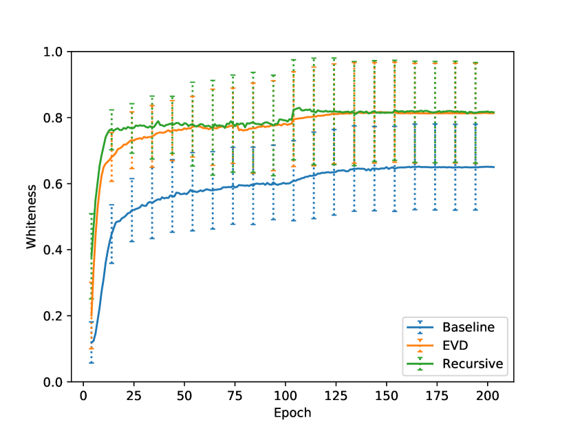
where in the extreme case of a diagonal ${\mathbf{\Phi}_{y}}$ we get $\rho=1$, and in the other extreme case of ${\mathbf{y}_{n}}$ being completely correlated we get $\rho=\frac{1}{M}$. We average the $\kappa$ and $\rho$ over all layers. The testing accuracy, the average normalized rank and average whiteness of features covariance for ResNet-110 and ResNet-50 are respectively depicted in Figs. 1(a), 1(b), 1(c) and Figs. 2(a), 2(b), 2(c). We capture the variability of the normalized rank and whiteness across different whitening layers, and also depict its standard-error boundaries. As expected, from the normalized rank Figs. 1(b),2(b) and the whiteness Figs.  1(c),2(c) it is evident that the whitening methods obtain a consistently higher rank and higher whiteness than the baseline methods. Considering the accuracy figures, it is noticeable that the whitening methods converge faster, and are more stable and less noisy. The converged accuracy of the baseline, EVD and recursive whitening methods is respectively $73.0\%$, $73.5\%$ and $73.0\%$ for ResNet-110 and $75.7\%$, $75.9\%$ and $76.0\%$ for ResNet-50. I.e., the whitening methods are on par or slightly better than the baseline method.

Two novel methods for whitening the features, named EVD and recursive gradient-based feature whitening, have been proposed. The methods offer reduced complexity compared to the direct feature whitening method [7], by applying the transformation to the weight gradients instead of to the activations and their gradients. The recursive method further saves computations by replacing the EVD-based transformation with a recursive transformation, updated in steps, treating only one subspace per step and designed to gradually reduce the condition number of the features covariance-matrix. The proposed methods are applied too ResNet-110 and ResNet-50 and obtain state of the art convergence in terms of speed, stability and accuracy.

References

- [1] Hirotugu Akaike. A new look at the statistical model identification. IEEE transactions on automatic control, 19(6):716–723, 1974.
- [2] Shun-Ichi Amari. Natural gradient works efficiently in learning. Neural computation, 10(2):251–276, 1998.
- [3] Anna Barnov, Vered Bar Bracha, and Shmulik Markovich-Golan. QRD based MVDR beamforming for fast tracking of speech and noise dynamics. In 2017 IEEE Workshop on Applications of Signal Processing to Audio and Acoustics (WASPAA), pages 369–373. IEEE, 2017.
- [4] Anthony J Bell and Terrence J Sejnowski. The “independent components” of natural scenes are edge filters. Vision research, 37(23):3327–3338, 1997.
- [5] Nils Bjorck, Carla P Gomes, Bart Selman, and Kilian Q Weinberger. Understanding batch normalization. In Advances in Neural Information Processing Systems, pages 7694–7705, 2018.
- [6] J. Deng, W. Dong, R. Socher, L.-J. Li, K. Li, and L. Fei-Fei. ImageNet: A Large-Scale Hierarchical Image Database. In CVPR09, 2009.
- [7] Guillaume Desjardins, Karen Simonyan, Razvan Pascanu, et al. Natural neural networks. In Advances in Neural Information Processing Systems, pages 2071–2079, 2015.
- [8] Gene H Golub and Charles F Van Loan. Matrix computations, volume 3. JHU press, 2012.
- [9] Simon S Haykin. Adaptive filter theory. Pearson Education India, 2005.
- [10] Kaiming He, Xiangyu Zhang, Shaoqing Ren, and Jian Sun. Deep residual learning for image recognition. In Proceedings of the IEEE conference on computer vision and pattern recognition, pages 770–778, 2016.
- [11] Lei Huang, Dawei Yang, Bo Lang, and Jia Deng. Decorrelated batch normalization. In Proceedings of the IEEE Conference on Computer Vision and Pattern Recognition, pages 791–800, 2018.
- [12] Sergey Ioffe and Christian Szegedy. Batch normalization: Accelerating deep network training by reducing internal covariate shift. arXiv preprint arXiv:1502.03167, 2015.
- [13] Agnan Kessy, Alex Lewin, and Korbinian Strimmer. Optimal whitening and decorrelation. The American Statistician, 72(4):309–314, 2018.
- [14] Alex Krizhevsky, Geoffrey Hinton, et al. Learning multiple layers of features from tiny images. 2009.
- [15] Yann Le Cun, Ido Kanter, and Sara A Solla. Eigenvalues of covariance matrices: Application to neural-network learning. Physical Review Letters, 66(18):2396, 1991.
- [16] Yann A LeCun, Léon Bottou, Genevieve B Orr, and Klaus-Robert Müller. Efficient backprop. In Neural networks: Tricks of the trade, pages 9–48. Springer, 2012.
- [17] Daniel Povey, Xiaohui Zhang, and Sanjeev Khudanpur. Parallel training of deep neural networks with natural gradient and parameter averaging. arXiv preprint arXiv:1410.7455, 2014.
- [18] Tapani Raiko, Harri Valpola, and Yann LeCun. Deep learning made easier by linear transformations in perceptrons. In Artificial intelligence and statistics, pages 924–932, 2012.
- [19] Simon Wiesler and Hermann Ney. A convergence analysis of log-linear training. In Advances in Neural Information Processing Systems, pages 657–665, 2011.