Feature Importance Ranking for Deep Learning

Suppose ${\cal D}=\{{\cal X},{\cal Y}\}$ is a dataset used for supervised learning. In this data set, $(\boldsymbol{x},\boldsymbol{y})$ is a training example, where $\boldsymbol{x}\in{\cal X}$ is a vector of $d$ features and $\boldsymbol{y}\in{\cal Y}$ is its corresponding target. Let ${\boldsymbol{m}}\in{\cal M}$ denote a $d$-dimensional binary mask vector of $0/1$ elements, where $||{\boldsymbol{m}}||_{0}=s$, $s<d$ and $|{\cal M}|=\binom{d}{s}$. Thus, we can use such a mask vector to indicate a feature subset: $\{{\boldsymbol{x}}\otimes{\boldsymbol{m}}\}_{{\boldsymbol{x}}\in{\cal X}}$, where $\otimes$ denotes Hadamard product that yield a subset of $s$ features for any instance ${\boldsymbol{x}}\in{\cal X}$. Assume that ${\cal Q}({\boldsymbol{x}},{\boldsymbol{m}})$ quantifies the instance-level performance of a learning system trained on ${\cal D}$ via a feature subset, $\{{\boldsymbol{x}}\otimes{\boldsymbol{m}}\}_{{\boldsymbol{x}}\in{\cal X}}$, the feature importance ranking (FIR) can then be formulated as follows:

where ${\boldsymbol{m}}^{*}$ is the indicator of an optimal feature subset discovered by an FIR algorithm and ${\rm Score}({\boldsymbol{m}}^{*})$ quantifies the importance of all the selected features in this optimal subset.

Ideally, an FIR approach should be able to: 1) detect any functional dependence between input features and targets; 2) rank the importance of all the selected features to reflect their contributions to the learning performance; and 3) preserve the detected functional dependence and the feature importance ranking in test data.

To tackle the FIR problem stated in Eq.(1) effectively with three criteria described in Sect. 3.1, we propose a deep learning model of dual nets, operator and selector, as shown in Fig. 1(a). The operator net is employed to accomplish a supervised learning task, e.g., classification or regression, on a given feature subset provided by the selector net, while the selector net is designated to learn finding out an optimal feature subset based on the performance feedback of the operator net working on optimal feature subset candidates during learning. Both the operator and the selector nets are trained jointly in an alternate manner (c.f. Sect. 3.3) to reach a synergy for the FIR.

Technically, the operator is carried out with a deep neural network parameterized with $\theta$, $f_{O}(\theta;\boldsymbol{x},\boldsymbol{m})$, for a given task, e.g., multi-layer perceptron (MLP) or convolution neural network (CNN). This net is trained on ${\cal D}$ based on different feature subsets to learn $f_{O}\!:{\cal X}\times{\cal M}\rightarrow{\cal Y}$. After learning (c.f. Sect. 3.3), the trained operator net, $f_{O}(\theta^{*};\boldsymbol{x},{\boldsymbol{m}}^{*})$, is applied to the test data for prediction, where $\theta^{*}$ is the optimal parameters of the operator net and $\boldsymbol{m}^{*}$ is generated by the trained selector net (c.f. Sect. 3.4).

In our method, the selector is implemented with an MLP parameterized with $\varphi$, $f_{S}(\varphi;\boldsymbol{m})$. As defined in Eq.(1), a selected optimal feature subset should maximize the averaging performance of the operator quantified by ${\cal Q}({\boldsymbol{x}},{\boldsymbol{m}})$ for all $\boldsymbol{x}\in\cal X$. Thus, we want the selector net to learn predicting the averaging performance of the operator net on different feature subsets; i.e., $f_{S}\!\!:{\cal M}\rightarrow\mathbb{R}$. After being trained properly (c.f. Sect. 3.3), we can use an algorithm working on the trained selector net of the optimal parameters $\varphi^{*}$, $f_{S}(\varphi^{*};\boldsymbol{m})$, to generate an optimal feature subset indicated by ${\boldsymbol{m}}^{*}$ and rank feature importance to achieve ${\rm Score}({\boldsymbol{m}}^{*})$ (c.f. Sect. 3.4).

In essence, the FIR defined in Eq.(1) is a combinatorial optimization problem. According to the no free lunch theory for optimization [19], no algorithm can perform better than a random strategy in expectation in the setting of combinatorial optimization. Therefore, our learning algorithm is developed by leveraging learning with a stochastic local search procedure enhanced by injecting noise [20] on a small number of candidate feature subsets, ${\cal M}^{\prime}\subset{\cal M}$, to avoid the exhaustive search.

For a training data set, ${\cal D}=\{\cal X,\cal Y\}=\big{\{}(\boldsymbol{x},\boldsymbol{y})\big{\}}_{\boldsymbol{x}\in{\cal X},\boldsymbol{y}\in{\cal Y}}$, a mask subset, ${\cal M}^{\prime}$, converts each training example $(\boldsymbol{x},\boldsymbol{y})\in{\cal D}$ into $|{\cal M}^{\prime}|$ examples: $\big{\{}(\boldsymbol{x}\otimes\boldsymbol{m},\boldsymbol{y})\big{\}}_{\boldsymbol{m}\in{\cal M}^{\prime}}$. Thus, the loss functions on ${\cal M}^{\prime}$ (changing during learning) for the operator and the selector nets are defined respectively as follows:

Here, $l(\boldsymbol{x}\otimes\boldsymbol{m},\boldsymbol{y};\theta)$ is an instance-level cross-entropy/categorical cross-entropy loss for binary/mutli-class classification or the mean square error (MSE) loss for regression. In Eq.(2b), we utilize the loss of the operator net, $l(\boldsymbol{x}\otimes\boldsymbol{m},\boldsymbol{y};\theta)$, to characterize its learning performance, ${\cal Q}({\boldsymbol{x}},{\boldsymbol{m}})$, since maximizing ${\cal Q}({\boldsymbol{x}},{\boldsymbol{m}})$ is equivalent to minimizing $l(\boldsymbol{x}\otimes\boldsymbol{m},\boldsymbol{y};\theta)$. As described in Sect. 3.2, during learning, the operator net relies on the selector net to provide an optimal subset of marks, ${\cal M}^{\prime}$, indicating different optimal feature subset candidates, while the selector net requires the performance feedback from the operator net, $l(\boldsymbol{x}\otimes\boldsymbol{m},\boldsymbol{y};\theta)$ for all $\boldsymbol{m}\in{\cal M}^{\prime}$. Two nets in our learning model hence have to be trained alternately. Below, we present the main learning steps in our learning algorithm of two phases, while the pseudo code can be found from Sect. D in supplementary materials.

After the learning described in Sect. 3.3 is accomplished, we obtain the optimal parameters of the operator and the selector nets, $\theta^{*}$ and $\varphi^{*}$.

By using the trained selector net, $f_{S}(\varphi^{*};\boldsymbol{m})$, we find out an optimal feature subset with the same procedure used in Phase II-A as follows: 1) starting with ${\boldsymbol{m}}_{0}=\big{(}\frac{1}{2},\cdots,\frac{1}{2}\big{)}$, calculate the gradient ${\boldsymbol{\delta}}_{{\boldsymbol{m}}_{0}}={\frac{\partial f_{S}(\varphi^{*};\boldsymbol{m})}{\partial{\boldsymbol{m}}}}|_{{\boldsymbol{m}}={\boldsymbol{m}}_{0}}$; 2) finding top $s$ features by $({\boldsymbol{m}}^{*},\bar{\boldsymbol{m}}^{*})={\rm argsort}({\boldsymbol{\delta}}_{{\boldsymbol{m}}_{0}},s)$, where ${\boldsymbol{m}}^{*}$ indicates the optimal subset of top $s$ features; and 3) going through the validation procedure described in Phase II.A to ensure the optimality of ${\boldsymbol{m}}^{*}$. Thus, feature importance ranking on the final ${\boldsymbol{m}}^{*}$ is done by setting ${\rm Score}({\boldsymbol{m}}^{*})={\frac{\partial f_{S}(\varphi^{*};\boldsymbol{m})}{\partial{\boldsymbol{m}}}}|_{{\boldsymbol{m}}={\boldsymbol{m}}^{*}}$ and sorting the input gradients of selected features.

During test, for a test instance, $\hat{\boldsymbol{x}}$, the trained operator net, $f_{O}(\theta^{*};\boldsymbol{x},{\boldsymbol{m}})$, can be used to make a prediction, $f_{O}(\theta^{*};\hat{\boldsymbol{x}},{\boldsymbol{m}}^{*})$, via $\hat{\boldsymbol{x}}\otimes{\boldsymbol{m}}^{*}$, which allows a supervised learning task to be done based on only the optimal feature subset, ${\boldsymbol{m}}^{*}$, found out with our proposed approach.

Our first evaluation employs 3 synthetic datasets in literature [17, 11] for feature selection regarding regression and binary/multiclass classification as follows:

For each dataset, we randomly generate 512 and 1024 examples, respectively, for training and test. With our problem formulation described in Sect. 3.1, our experiment on synthetic data simulates an application scenario that selects $s$ out of $d$ features where $s$ is larger than the number of features relevant to the target in a dataset. As there are up to 4 relevant features in the above 3 datasets, we choose $s=5$ in our experiment and compare with all the methods reviewed in Sect. 2, including DFS [7], AvGrad [12], FS [11] based on MLP, LASSO [9], RF [16], RFE [2], BAHSIC [4, 5], mRMR [18] and CCM [17]. According to a taxonomy [3], DFS, AvGrad, RF and ours are embedding methods, FS is a wrapper method and all the others are filtering methods. For those filtering methods, we use the exactly same kernel SVM/SVR described in those papers [2, 4, 18, 5, 17] and an MLP on LASSO for classification/regression. While DFS, AvGrad, LASSO and RF work on FIR for all 10 features, all other methods work with the same setting as ours by finding out top 5 features and FIR.

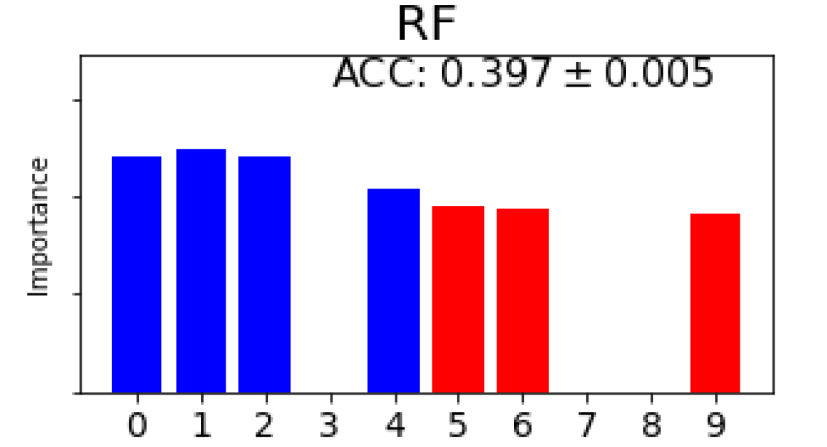
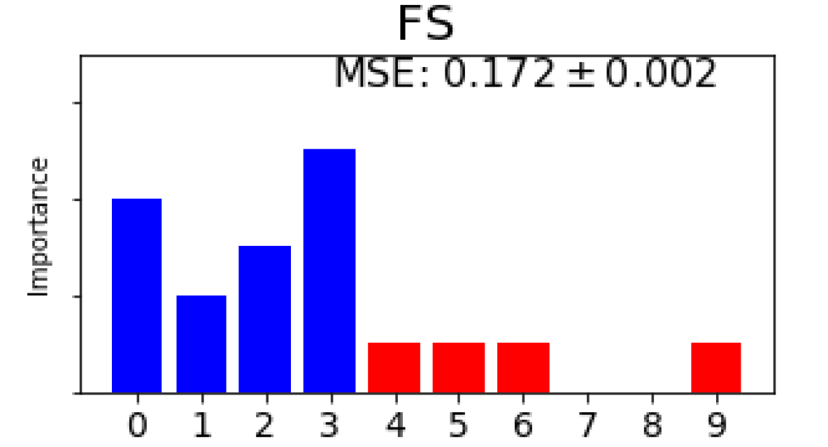
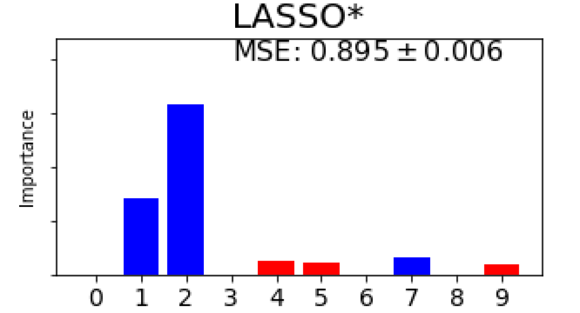
Fig. 3(b) shows the feature selection and FIR results yielded by different methods regarding top 5 features on 3 synthetic datasets where the FIR scores are normalized in each method and the equal FIR score is set to all the features selected by those methods without considering FIR. It is observed from Fig. 3(b) that our approach always finds out those relevant features in all 5 folds and does FIR properly by assigning negative scores (gradients), meaning unimportant, to irrelevant features. For the 4-way classification, DFS, RF, RFE, BAHSIC and CCM also find 3 relevant features in all 5 folds but others fail as shown in Fig. 3(b)(a) although mRMR and CCM cannot yield FIR scores. In terms of accuracy, ours outperforms all other 9 methods despite the fact that DFS, AvGrad and RF work directly on the full feature set. For the nonlinear regression, FS, RF, RFE and CCM also select 4 relevant features in all 5 folds but ours yields the least MSE as shown in Fig. 3(b)(b). For the binary classification, all the methods apart from LASSO find 4 relevant features in all 5 folds, as shown in Fig. 3(b)(c). For this dataset, those state-of-the-art filtering methods yield better accuracy than others and the accuracy resulting from ours is slightly worse but comparable to those. In terms of FIR on all relevant features, ours is entirely consistent with those yielded by RF but performs significantly better than RF on 3 datasets. In comparison to the existing FIR methods for deep learning, ours always outperforms DFS, AvGrad and FS on 3 datasets in terms of both FIR and learning performance.

We further evaluate our approach on several well-known benchmark datasets from two different perspectives; i.e., explainability of FIR and learning performance on supervised feature selection. Evaluation on more benchmark datasets can be seen from Sect. B in Supplementary Materials.

We finally evaluate our approach on a real-world enhancer–promoter data, a challenging task that classifies the function of DNA sequences into enhancer, promoter and background [25]. As listed in Table 1, the data used in this experiment are sampled from annotated DNA regions of GM12878 cell line (200 dp), the same as used in DFS [7], a feature selection method dedicated to this task. For comparison, we also apply DFS as well as RF and RFE, 2 strongest FIR methods manifested in our experiments, to this dataset. The same MLP architecture is used in implementing DFS and the operator net in our model. Fig. 6 shows accuracies and the FIR scores of top $s=35$ out of $d=102$ features yielded by 4 different methods and those features colored in red correspond to the genes of which functions are well known in medicine and genetics literature (see Table 2 in [7] for details). In terms of accuracy, ours is comparable to DFS and slightly better than RF and RFE, where the test accuracies of RFE and ours are based on $35$ features but the accuracies of RF and DFS are achieved with all 102 and 94 features selected by DFS via weight shrinkage, respectively. As seen in Fig. 6, those top features ranked by DFS and ours, two deep learning methods, appear quite similar but significantly different from those top features ranked by RF and RFE. The biological implication resulting from the results shown in Fig. 6 is worth investigating further from a biological/medical perspective. More results on this dataset can be found from Sect. C in Supplementary Materials.

Regarding our alternate learning algorithm, our empirical studies suggest that it generally converges by reaching a local optimum (see Sects. B and C in Supplementary Materials for details).

References

- [1] W. Samek, T. Wiegand, and K. R. Müller. Explainable artificial intelligence: Understanding, visualizing and interpreting deep learning models. arXiv preprint arXiv:1708.08296, 2017.
- [2] I. Guyon, J. Weston, and S. Barnhill. Gene selection for cancer classification using support vector machines. Machine Learning, 46(2):389–422, 2002.
- [3] I. Guyon and A. Elisseeff. An introduction to variable and feature selection. Journal of Machine Learning Research, 3(3):1157–1182, 2003.
- [4] L. Song, A. Smola, A. Gretton, K. M. Borgwardt, and J. Bedo. Supervised feature selection via dependence estimation. In International Conference on Machine learning, pages 823–830, 2007.
- [5] L. Song, A. Smola, A. Gretton, J. Bedo, and K. Borgwardt. Feature selection via dependence maximization. Journal of Machine Learning Research, 13(5):1393–1434, 2012.
- [6] S. Hooker, D. Erhan, P. J. Kindermans, and B. Kim. A benchmark for interpretability methods in deep neural networks. In Advances in Neural Information Processing Systems, 2019.
- [7] Y. Li, C. Y. Chen, and W. Wasserman. Deep feature selection: Theory and application to identify enhancers and promoters. Journal of Computational Biology, 23(5):322–326, 2016.
- [8] J. Weston, A. Elisseeff, and B. Scholkopf. Use of zero-norm with linear models and kernel methods. Journal of Machine Learning Research, 3(5):1439–1461, 2003.
- [9] R. Tibshirani. Regression shrinkage and selection via the LASSO. J. R. Stat. Soc. Series B Stat. Methodol., 58(2):267–288, 1996.
- [10] H. Zou and T. Hastie. Regularization and variable selection via the elastic net. J. R. Stat. Soc. Series B Stat. Methodol., 67(2):301–320, 2005.
- [11] J. Friedman, T. Hastie, and R. Tibshirani. The Element of Statistical Learning. Springer, Berlin, 2001.
- [12] H. Yotam. Interpretation of prediction models using the input gradient. ArXiv: 1611.07634, 2016.
- [13] M. T. Ribeiro, S. Singh, and C. Guestrin. Why should I trust you?: Explaining the predictions of any classifier. In Proceedings of the 22nd ACM SIGKDD international conference on knowledge discovery and data mining, pages 1135–1144. ACM, 2016.
- [14] I. van der Linden, H. Haned, and E. Kanoulas. Global aggregations of local explanations for black box models. In Proceedings of SIGIR Workshop on Fairness, Accountability, Confidentiality, Transparency, and Safety, 2019.
- [15] B. Skrlj, S. Dzeroski, N. Lavrac, and M. Petkovic. Feature importance estimation with self-attention networks. In Proceedings of 24th European Conference on Artificial Intelligence, 2020.
- [16] L. Breiman. Random forests. Machine Learning, 45(1):5–32, 2001.
- [17] J. Chen, M. Stern, M. Wainwright, and M. Jordan. Kernel feature selection via conditional covariance minimization. In Advances in Neural Information Processing Systems, 2017.
- [18] H. Peng, F. Long, and C. Ding. Feature selection based on mutual information criteria of max-dependency, max-relevance, and min-redundancy. IEEE Transactions on Pattern Analysis and Machine Intelligence, 27(8):1226–1238, 2005.
- [19] D. H. Wolpert and W. G. Macready. No free lunch theorems for optimization. IEEE Transactions on Evolutionary Computation, 1(1):67–82, 1997.
- [20] O. J. Mengshoel. Understanding the role of noise in stochastic local search: Analysis and experiments. Artificial Intelligence, 172(2):955–990, 2008.
- [21] Y. LeCun, C. Cortez, and C. Burges. The MNIST Handwritten Digit Database. http://yann.lecun.com/exdb/mnist/.
- [22] D. Dua and C. Graff. UCI Machine Learning Repository. http://archive.ics.uci.edu/ml.
- [23] J. Li, K. Cheng, S. Wang, F. Morstatter, R. P. Trevino, J. Tang, and H. Liu. Feature selection: A data perspective. ACM Computing Surveys, 50(6):94, 2018.
- [24] Yale Face Database. http://vision.ucsd.edu/content/yale-face-database.
- [25] R. Anderson, C. Gebard, I. Miguel-Escalada, et al. An atlas of active enhancers across human cell types and tissues. Nature, 507:455–461, 2014.
- [26] N. Srivastava, G. Hinton, A. Krizhevsky, I. Sutskever, and R. Salakhutdinv. Dropout: A simple way to prevent neural networks from overfitting. Journal of Machine Learning Research, 15(8):1929–1958, 2014.
- [27] B. Xue, M. Zhang, W. N. Browne, and X. Yao. Survey on evolutionary computation approaches to feature selection. IEEE Transactions on Evolutionary Computation, 20(4):606–626, 2016.
- [28] M. Tan and Q. V. Le. EfficientNet: Rethinking model scaling for convolutional neural networks. In Proceedings of the 36th International Conference on Machine Learning, 2019.
- [29] M. Yuan and Y. Lin. Model selection and estimation in regression with grouped variables. J. R. Stat. Soc. Series B Stat. Methodol., 68(1):49–67, 2006.