Fault-tolerant resource estimation using graph-state compilation on a modular superconducting architecture
Abstract
The development of fault-tolerant quantum computers (FTQCs) is gaining increased attention within the quantum computing community. Like their digital counterparts, FTQCs, equipped with error correction and large qubit numbers, promise to solve some of humanity’s grand challenges. Estimates of the resource requirements for future FTQC systems are essential to making design choices and prioritizing R&D efforts to develop critical technologies. Here, we present a resource estimation framework and software tool that estimates the physical resources required to execute specific quantum algorithms, compiled into their graph-state form, and laid out onto a modular superconducting hardware architecture. This tool can predict the size, power consumption, and execution time of these algorithms at as they approach utility-scale according to explicit assumptions about the system’s physical layout, thermal load, and modular connectivity. We use this tool to study the total resources on a proposed modular architecture and the impact of tradeoffs between and inter-module connectivity, latency and resource requirements.
Rapid progress toward developing FTQCs has promised a new era where universal and million-qubit machines may outperform digital computers in solving specific problems (see [1, 2, 3] for some recent overviews and developments). Meanwhile, the size, connectivity, and fidelity of today’s highly-noise-sensitive qubit devices constantly improve [4, 5]. These platforms can already be considered the building blocks of early FTQCs, which use redundancy to suppress noise – a process known as quantum error correction (QEC) [6, 7, 3, 8].
However, designing and implementing hardware-resource-efficient, application-specific, error corrected protocols remains a fundamental challenge to unlocking the fault-tolerant (FT) era. While the complexity and scaling behaviors for foundational FT algorithms such as Shor[9], quantum signal processing[10] (QSP), and ground state energy estimation[11] (GSEE) are well understood, the resources required when these algorithms are applied to specific practical problems is an important open question. Moreover, the overheads and space-time resource requirements for physical hardware are even less well understood and depend on a myriad of choices of platform and micro-architectures. This is further complicated by specific choices to tailor algorithms to particular hardware, which makes comparison across algorithms, hardware platforms, and architectures challenging.
FT hardware resource estimations can be presently derived through some well-established tools[12, 13, 14, 15, 16]. However, such tools primarily focus on a method called the “T-counting method”. One of the core mechanisms in many of these tools is to count the number of non-Clifford components in the input algorithm and scale space-time resources accordingly. More precisely speaking, these start with different types of high-level pre-compilation and gate transpilation steps, then synthesize the logical circuit into Clifford+T or similar, re-scale everything with a desired level of parallelization, perform logical-level computations (FT-compilations) to get the intermediate representation, and calculate space-time quantities based on the T-count, depth, or similar. There are subtle differences in how such footprint-style approaches perform logical-level operations, including surface code, lattice surgery, and T-gate distillation computations. However, they commonly lack tailored estimates specific to QPU layouts, robust estimations of surface code distance, and overestimate the upper bounds of space-time resources.
In contrast, we present a method, open-source repository, and superconducting-qubit-informed architectural model for estimating the resources required to execute specific applications. The goal is to aid the design and feasibility assessment of next-generation FT devices and quantify the trade offs for specific hardware implementations.
I Methods: Graph-state-based Architecture Design and Resource Estimations
Our approach to superconducting FT-hardware resource estimation is based on graph-state compilation of logical algorithms as proposed in [17, 18, 19, 20, 21, 22], and subsequently refined below. In this approach, a quantum circuit is compiled into a graph-state resource (called an algorithm-specific graph-state in [19]) to be consumed by a schedule of specific measurements.
Using an algorithm-specific graph-state , the original unitary/circuit can be implemented deterministically by applying only single qubit measurements with classical feedforward. This describes a Measurement Based Quantum Computing (MBQC) pattern, an approach initially proposed in [20, 23]. MBQC is an appealing framework for distributed FTQC since only an algorithmic specific resource (eg: a the graph-state) and measurements on logical qubits are required to be specified. Below, we discuss and employ a specific form of MBQC[24, 19] for compilation purposes. The preparation of the graph-state resource is carried out via entangling operations on a single bus of ancilla qubits. Clifford operations are abstracted away, classically simulated, and converted into the graph-state resource. In this this work we apply this framework to understand the resources needed to execute large-scale quantum algorithms on a exemplar superconducting qubit architecture.
Consider a mathematical graph defined by a set of vertices and a set of edges. The graph-state corresponding to this graph can be constructed by associating each vertex to a qubit and each edge to an entangling operation between the qubits represented by the edge’s vertices. For brevity, we will often use the term “node” when discussing the qubit that a vertex represents. Nodes will be assigned measurements in a non-Clifford basis corresponding to the non-Clifford gates in the original circuit. A set of schedules for preparing the graph-state, performing non-Clifford measurements, and tracking Pauli corrections are required to execute the circuit fully. We denote the nested set of stabilizer measurement schedules that prepares the graph for computations as . The other nested set of non-Clifford measurement schedules “consumes” the graph-state and is denoted . Both schedules contain a list of subsets specifying the order of measurements, where each subset hosts the list of nodes meant to be measured simultaneously.
Preparing the graph-state per , then performing single qubit measurements to consume the graph per , while accounting for the tracked Pauli corrections on the software, will essentially execute the complete FT algorithm.
For large-scale computational workflows, there are limits to the amount of computation that can be done on a single processor in a given time, owing to the amount of processing power that can be fit onto an individual die. These restrictions can ultimately be traced back to physical limitations and manufacturing yield. As a result, computations are often broken up across many processors and machines, where penalties imposed from higher latency or reduced bandwidth are balanced to leverage increased raw computational ability. Here, we make an analogy to distributed FTQC, which consists of connected compute modules. The computational power of each module has been constrained by yield. These operational (thermal) or manufacturing constraints limit the number of qubits that can be fabricated into a single quantum processing unit (QPU). In contrast to the flexible connectivity and relatively slow speed between compute modules, the QPUs have a fixed native connectivity and faster gate speed. In section I.3, we will physically motivate the number of qubits in a single compute module to be the order of one million qubits. We propose that such modules will be interconnected more sparsely with reduced fidelity, bandwidth or entangling gate speed. We describe a connection between modules of code distance as a single pipe and abstract the transduction efficiency away as an interaction time, known as the inter-module tock. Here, we can quantify the impact of this time on the total algorithm runtime.
At a high level, this paper describes the following process: the ingestion of an algorithm that consists of a set of single and two-qubit gates, segmenting this algorithm into recurring sub-circuits called widgets, computing the graph properties of these widgets and scheduling the preparation and consumption of these widgets on a specific hardware architecture, described in detail. We will explain the architectural model, its parameters, and how this architectural model can be tailored to particular hardware constraints in section I.3.
In the remainder of this section, we first detail our methodology to compile and estimate FT resources based on user inputs in section I.1. We then describe the logical or macro-architecture in section I.2 followed by the details of our hardware or micro-architecture in section I.3. More information on the I/O, estimation pipeline, and configurations used in RRE are presented separately in section A.1.2.
I.1 Modular graph-state-based compilation and estimations
Assume the user possesses a known, fixed description of their logical and hardware architecture, denoted by a set of configuration parameters, . The user also possess a circuit, , which implements a unitary operator, , acting on algorithmic qubits. That is,
| (1) |
In practice, this is a quantum instruction set with potentially tens of millions of gates. We denote the diamond-norm precision for gate synthesis as . Further, we denote the number of logical and gates in excluding the ones implicitly residing in the arbitrary-angle non-Clifford rotation gates as , and as the number of non-Clifford arbitrary-angle gates in including the ones implicitly residing in other logical gates. Finally, we assume fault-tolerant execution using rotated surface code with distance .
As mentioned, we are considering a MBQC framework, using graph-state compilation to specify circuit execution. One advantage of this approach is that one does not require the entire graph-state, , to be initialized on the MBQC at all times [25]. Rather, one is able to break the circuit execution into steps and specify the parts of the graph-state that need to be present at a particular step by using three schedules; a schedule for graph-state preparation, , a schedule for graph-state consumption, , and a schedule for measurement basis, .
and can be considered nested sets, where subsets list the nodes required to be measured at each step. For example, a five-step consumption schedule for a graph of 56 nodes may look like
| (2) |
is a nested list identifying which rotational basis ( or for small arbitrary angles) must be used for parity measurements of the nodes at the distillation-consumption stage per each step of . This provides a natural separation between two distinct node types: and -nodes.
Note that the the number of nodes comprising the graph, , is typically much larger than the number of input qubits. That is, . This is due to the fact that ancillary qubits are always added for an MBQC realisation of a given quantum algorithm. However, due to the aforementioned scheduling only a relatively small subset of logical qubits, representing each node, are required at any step to execute . The maximum number of logical qubits required at any step is denoted . This is also referred to as the maximum quantum memory. Typically [26]. Note that the number of nodes in the graph are never lower than the total number of algorithmic input qubits [27], using the MBQC framework at the logical level simplifies the Clifford and non-Clifford compilation of the circuit.
One should also be aware that distinct graph-states with similar attributes can be constructed from different states, however for resource estimation purposes, we always consider the graph-state constructed from . Arbitrary inputs to algorithmically specific graphs can be generated by first compiling the graph assuming a zero input and then appending appropriate ancilliary nodes to perform teleportation into the specific input nodes of one graph from the output nodes of another [25]
Given the above descriptions, we argue that resource estimations can be performed if one provides a set of resource estimation primitives,
| (3) |
where we have explicitly denoted the aforementioned required user inputs on the left-hand side, which generate the set of primitives used for resource estimation shown on the right. It is inefficient to directly compile a utility-scale with tens of millions of gates and considerable circuit depth for resource estimations or the execution on the hardware. It is highly challenging to construct exactly for enormous, utility-scale circuits. Instead, the resource estimation set, , was approximately constructed and robustly verified following the steps below.
I.1.1 Input circuit widgetization and our stitching strategy
Due to the size of a utility-scale input circuit, a decomposition strategy is required to avoid memory bottlenecks on RRE. Fortunately, quantum algorithms often comprise repeating blocks, which facilitate decomposing them.

Our decomposition strategy is to slice in the time direction into “widgets” (or subcircuits) of -width with a user-defined maximum allowed depth of . We emphasize there are no entangling gates connecting the subcircuits. One could then execute the complete algorithm as a sequence of the subcircuits, where
| (4) |
where we have defined and . We call this process “circuit widgetization”, pictured in fig. 1, which allows us to avoid the memory overheads associated with decomposing the complete circuit to elementary operations. Notice the particular choice of widgetization above is likely not optimized for reducing space-time costs; however, it was selected due to the ease of implementation.
After the widgetization process, one can construct an approximate version of . We propose and verify a widgetization-based set below as a good approximation of for resource estimation purposes,
| (5) |
In this widgetization-based estimation procedure, we first obtain estimation primitives for each widget based on its graph and then define the full circuit resources estimates as,
| (6) |
where is the graph-state compiled from the th widget. eq. 6 highlights the critical assumptions we made while generating all the estimations in this work and formally states our “stitching” strategy. We stitch the individual graphs and scheduling lists to approximate the complete , , , and . Note that while literal stitching of the widgets would be required to execute the circuit on a MBQC, it is not required for resource estimation purposes [25]. The computational requirements required for obtaining resource estimates can thus be reduced by calculating the “widgetized" quantities above on the software.
I.1.2 Pre-processing the input subcircuits
To prepare for graph compilation each widget must be parsed and transpiled so that it only contains logical Clifford++ using exact gate equivalences. Here, ’s are nontrivial small angles. Later on, when we want to perform single qubit logical measurements, at the end during the distillation-consumption stage, each node needs to be decomposed to a chain of Clifford+ itself – a process sometimes referred to as gate synthesis[28, 29].
The transpilation to logical Clifford++ is also performed by RRE. Performing gate synthesis at the end allows us to generate, cache, and reuse subgraphs independent from logical and hardware-level configurations, .
Once transpilation is complete, we need to generate the unified sets of graph states and schedules , , and (and some other intermediary lists detailed below), which we argue suffice for the resource estimations of .
I.1.3 Jabalizer FT-compiler: generating MBQC sets
RRE employs the stabilizer-tableau-based Jabalizer FT-compiler[30] as an essential intermediate layer to transform individual logical subcircuits into corresponding subgraphs, consumption schedules, MBQC-formatted circuits, and other critical information. In particular, each MBQC-formatted circuit is an optional qasm output of the Jabalizer that corresponds to a completely positive trace-preserving (CPTP) map transforming the larger space of all graph qubits to the smaller space of (i.e. equivalent to the execution of ). The circuit is extracted from the corresponding graph, Pauli corrections, and the consumption schedule and contains logical , Phase and gates, as well as mid-circuit measurements. We refer readers to [30, 24, 19] for complete details on the different components of Jabalizer’s scalable compilation method.
Given an individual logical subcircuit , containing only Clifford++, Jabalizer can generate the following set of quantities,
| (7) |
Here, is a set tracking in which Pauli corrections (frames) must be applied to the measurements at the end. denotes the set or map of output nodes in the graph state. Because we decompose the complete algorithm in the time with a uniform width covering all qubits, the number of intermediate input and output nodes are always the same, so knowing are not required for resource estimation purposes. is the maximum quantum memory needed to process . is the graph consumption schedule to perform individal logical qubit measurements. is the list identifying which rotational basis must be used for each of the logical measurements. Finally, is the MBQC-formatted qasm extracted from the previous outputs, which corresponds to an CPCT map from graph to output qubits executing the corresponding portion of the logical algorithm. For the widget in step , this correspondence can be written as .
I.1.4 Substrate Scheduler library: generating preparation schedules
RRE employs the Substrate Scheduler [31] to map the graph states , calculated by Jabilizer in eq. 7, to the set of graph initialization schedules . These initialization schedules are optimized for the quantum bus in the superconducting hardware layout detailed in section I.3. We assume the bus contains linear arrangements of surface code data qubits to store the graph alongside a linear ancillary system. The bus is laid out in comb-like patterns in the cryogenic modules, facilitating the measurements. The Substrate Scheduler currently finds an optimum schedule based on an input of individual mapping to this layout. The operation of the scheduler can be improved by including additional information on node types and adding support for customized bus architecture in the future.
I.1.5 Verification protocol for the individual graphs
The robust verification of our compilation and estimation methodology at different layers was a priority when designing RRE. To this end, we have developed a verification protocol, fig. 2, to precisely check the correctness of individual subgraphs as long as the widgets originated from small circuits with 10’s of logical qubits.

Following the process shown in the fig. 2, the input logical unitary, (e.g. a small algorithm or a subcircuit of a bigger one in the qasm format), is provided to the test module. As detailed above, RRE facilitates running Jabalizer on the input to output a unified JSON containing the graph state, consumption schedule, and Pauli tracking information. The MBQC-formatted qasm for is particularly relevant to the verification protocol, which we label with in the figure to highlight the correspondence discussed earlier. Now, independent from the operations of the compiler, one can build the inverse of the original algorithm for small-size cases, i.e. . For example, if is unitary for a logical QFT4, then is InverseQFT4 manually generated. We then use a quantum simulator software to run noiseless simulations of the staggered circuit instructions shown in the lowest panel of fig. 2 with the input state of the verification protocol set, as an example, to . By the unitarity principles, if the was valid (which implies the validity of the graph state and the rest of Jabalizer outputs), then simulation output counts must exactly correspond to for the example input.
We have successfully simulated and verified graphs produced in RRE as per fig. 2 for several small-size input circuits containing QFT, single TOFFOLI, and Clifford instructions (where some were widgetized from larger algorithms) for all possible input stats as
| (8) |
I.1.6 Space-optimal resource estimation
In this section, we formulate the space-time volume requirements for graph state processing parts based on , , and the architecture detailed in section I.3.
We consider an architecture with spatially optimal quantum bus and time-optimal compilation strategies. The architecture contains two fridges based on the assumption that superconducting platforms have a low quantum cycle duration and would benefit from minimizing physical footprint and interleaving graph preparation and consumption. This means we always create surface code patches per linear register of the bi-linear bus (one line for data and another one for ancilla qubits). We arrange patches in a comb-like arrangement of the bi-linear bus for processing the subgraphs and hosting ancillae in the fridges. Any remaining space is always used to fit as many -factories fridge to service the bus. There will be an equal number of per each fridge – further details below.
The space-time volume of the complete graph creation on the bi-linear quantum bus before each single qubit logical measurement,
| (9) |
where is the sum of the sub-schedule lengths, for set . is the number of distinct measurement steps for the graph initialization part. For notational convenience we will extend and use this notation of for other sets as well.
| DistillWidget (superconducting) | Space | Qubits, | Cycles, | |
|---|---|---|---|---|
| (15-to-1)17,7,7 | 6472 | 4620 | 42.6 | |
| (15-to-1) (20-to-4)23,11,13 | 387155 | 43,300 | 130 | |
| (15-to-1) (20-to-4)27,13,15 | 382142 | 46,800 | 157 | |
| (15-to-1) (15-to-1)25,11,11 | 279117 | 30,700 | 82.5 | |
| (15-to-1) (15-to-1)29,11,13 | 292138 | 39,100 | 97.5 | |
| (15-to-1) (15-to-1)41,17,17 | 426181 | 73,400 | 128 |
We now detail how we select the class of -state distillation widgets placed in each modules, as described in fig. 4. We always choose the type of distilleries from widgets detailed by Litinski in Table 1 of [32]. Furthermore, we consistently assume a superconducting homogeneous physical error rate of for all quantum operations or, at least, for the dominant error rates, whether from measurements or two qubit physical gates. Therefore, from this table, we have extracted the widgets matching and summarized those in table 1 forming a “Widget Lookup Table”, which we recursively go through to find a suitable T-factory type. table 1 is part of that the user provides and can customize for RRE.
table 1 details a selection of distillation widgets numerically simulated in [32]. The following are important for the “lookup table”: The output probability, , sets the error rate for the ancilla state and bounds the error rate on any T-gate implemented using the ancilla. The number of qubits, 2D patch dimensions, and physical cycle sweeps depend on the widget construction. We have only considered the selection of distillation widgets that produce -states (hence ignoring any entries for in the original table). In our architecture, we assume there are
| (10) |
distilleries per fridge servicing the widgets with purified T-states for each node as measured.
is the total number of physical qubits available for each QPU fridge, and is the number of physical qubits required for a distillery. The above ignores the geometrical considerations required to match fridge and widget structures. Such considerations are planned as improvements in future RRE versions.
Next, we must include the resource cost for the gate-synthesis decomposition to Clifford+ executed at the logical measurement step of each graph node, consuming resource states of the distillation factories, at the end of each subgraph processing step. We assume the graph nodes are either of the type requiring arbitrary -basis measurements or a single -basis one. The measurements that require a -axis rotation are decomposed into -gate sequences of length as instructed by the gate synthesis method available to RRE. is known as the diamond-norm error for decompositions to Clifford+ – see below and [29] for details.
For each distilled -state, cycles are needed to prepare the state, and is required to interact the state with the graph node and measure it in the or -basis. Hence for each node measurement, assuming an -basis measurements, the volume increases as . Hence, for all nodes of both types and that need to be measured sequentially, the space-time volume is
| (11) |
where we introduced , which is our proxy for the total number of gates, -count, and a quantity typically much larger than . Note that we do not have to include the space-time volume of the actual distillation widgets in the calculations as their errors are subsumed into the of the distilled state, specified in [32, Fig. 1]. In order to write the total space-time volume and simplicity of the estimation of , we assume the worst-case scenario of no parallelization coming from distilleries, which is equivalent to finding the largest volume and satisfying rate conditions with a single T-factory (we will revert to exploiting all possible distilleries for hardware time calculations). However, when widgets from table 1 are chosen to have a second (20-to-4) layer (the second and third widgets), we still replace and affecting the space-time volume, as the distillation widget produces 4-outputs simultaneously.
A single cycle time of the surface code has a failure probability governed by the following physical-to-logical rates scaling (e.g. see [6, 33]):
| (12) |
where the coefficients, and , are directly informed by Minimum Weight Perfect Matching (MWPM) decoder simulations and device modeling. In particular, decoder simulations provide logical and physical probabilities while we sweep through and consume one qubit and two qubit error rates and channels offered by device modeling – see section V for details. Consequently, a single unit cell containing cycles fails with probability
| (13) |
and failure rate of a volume of these cells is
Assuming that then , and thus and,
Subtracting each side from 1, and taking the logarithm of each side, this becomes,
| (14) |
We remind the reader that the total algorithm failure rate, , represents the failure probability of the entire space-time volume and, hence, the computation. This number is budgeted by the user. We now need to solve eq. 14, which can be rewritten,
| (15) |
where . The minimum code distance required is the smallest integer where the LHS of the above equation is negative. The only free variables above are the distillation widget’s cycle time, , and . Note and were previously extracted from Jabalizer, Pauli Tracker, and the Substrate Scheduler.
To determine and , we perform nested loops to iterate through widgets and then gate synthesis’ . The inner loop feeds back into the Clifford+ decomposition as the failure rate of a unit cell, , sets the approximation error as . By choosing a particular widget, we fix , which also fixes the distilled state’s output error rate, .
In a compiled quantum algorithm, we wish to ensure that the implemented -gates have precisely the same error rate as any other gates in the compiled circuit. A Pauli initialization or measurement takes a single unit cell in the space-time volume. Hence, its failure rate is governed by eq. 13. This error rate must be dominant. Consequently, the error output, , from the distillation circuit should be less than the failure rate of this cell (i.e., we must ensure that the output of distillation is at least as good as a unit cell in the space-time volume). Hence, we first choose the smallest value of from table 1 and solve eq. 15 for . We then check that, for a physical error rate of and our solution for if
| (16) |
is satisfied for the corresponding entry. If this is not satisfied, we must choose a better-performing state distillation widget in the outer loop. We move to the next entry on the list and repeat until we find a distillation widget that performs at least as well as the failure of a logical unit cell.
Once the particular distillation widget is chosen, our total number of required physical qubits and total intra-modular runtime, including first nonparallel graph preparation and all distillation-injection-consumption operations, can be calculated respectively as,
| (17) | |||||
where is the characteristic gate time (which sets the quantum tock of all intra-modular operations for the architecture), and . Note we only need to include the temporal cost of initializing the first subgraph with since the remaining graph preparations will be performed in parallel with distillation-consumption operations as demonstrated in the following section.
To validate the assumptions of the two-fridge architecture, detailed below, we must also verify that for each of scheduling steps, the preparation time for the upcoming subgraph is always greater than the cumulative time to perform intra-modular distillation-consumption operations. For every widget , these include distillation and transferring (injecting) -states, , and all surface code operations and parity measurements to consume graph nodes, . Formally,
| (18) |
In the above, we exploit the parallelization coming from multiple distilleries. and indicate the number of nonparallel surface code cycles at each stage. and denote the number of and -type nodes in the sub-step of the consumption schedule, respectively. Notice also .
The total FT-hardware time then becomes
| (19) |
where,
| (20) |
In the above, and is the characteristic time for the inter-modular operations to teleport Bell states needed to stitch and prepare the next subgraphs on the real FTQC. is the number or bandwidth of inter-modular pipes connecting fridges, each with a width of . Overall, is the cumulative time for the graph handovers, which scales by the number and the speed of inter-modular pipes. is the delay added to perform decoding, fully classically, for all QEC cycles. We suggest a method to estimate in section A.1.2 based on tensor network decoding[34, 35].
We have summarized the workflow as algorithm 1 below.
I.2 High-level architecture for modular graph state processing
To ultimately estimate resources for executing an FTQC algorithm and understand tradeoffs, we propose an architectural model, based on superconducting qubits. Here, we assume a physical layout of the FT computer that consists of sets of rotated surface code logical patches that correspond to the nodes of the graph, where each patch contains physical qubits.
The graph state processing described in I.1.1 leads naturally to an architecture where the hardware is divided into modules that handle the processing of these widgets in an interleaved fashion. In the steady state, the processing of the quantum algorithm itself consists of 3 steps: 1) graph preparation, 2) teleportation of output nodes from previous widget to the input nodes of the current widget, and 3) graph consumption.

This interleaved executing structure allows us to study a degree of parallelism in a distributed FTQC. As steps 1 and 3 of the graph state processing can be done simultaneously, we propose to split the preparation and consumption steps onto physically separate modules - alternating between two distinct modules to carry out the computation. The graph processing cycle consists of 2 steps: graph preparation and graph consumption where necessary T-rotations are applied to measurements, and graph consumption as depicted in fig. 3.
Perhaps the most scarce resource in universal FTQC is state distillation, and for the purposes of this study we propose an equal number of magic state distillation factories in each module to produce T-states. This leads to a high level architecture shown in fig. 4 with an example logical layout shown in fig. 7. Here, the faster native connectivity of a lattice of superconducting qubits can be exploited within a module, where reduced connectivity or slower interaction can be scheduled in the teleportation to connect output nodes from IO graph state widgets.

I.3 Hardware architecture based on superconducting qubits
This high level architectural concept informs an system level model, that at a minimum must contain:
-
1.
lattice of rotated surface code qubits
-
2.
register of logical qubits for graph creation and consumption each coupled to
-
3.
continuous bus of ancilla qubits for connecting graph state logical qubits and for teleporting T-states for consumption.
-
4.
quantum interconnect between modules to enable connection along the ancilla bus.
-
5.
Magic state distillation factories.
Importantly, as described in section I quantum algorithms are processed on a MBQC by a sequence of measurements and rotations of logical qubits facilitated by a bus of ancilla qubits. As a result, such an architecture requires cryostat modules only have connections along the bus of ancilla qubits. This drastically simplifies the hardware as dense, long range connectivity is not required between modules. The bare minimum requirement is that the number of coherent links along this bus only needs to be equal to the code distance, however adding additional connections will have the benefit of accelerating the overall computation. We will quantify this tradeoff in section III.
To account for required resources, we need physical specifications of the system. To gather these we start from the layout of the qubits. To provide the most relevant estimates to today’s hardware, base our estimates on a superconducting qubit architecture that consists of tunable transmon qubits coupled via tunable couplers[36]. This architecture has been implemented with high fidelity in a number of groups[37, 38, 39, 40]. Here we specify that the transmon qubits will be laid out in a square lattice and coupled to each other via tunable couplers. This square lattice corresponds directly to the surface code and allows us to relate qubit number to code distance directly.
To determine the number of qubits built into a single module and the overall size of the QPU in that module, we must determine the pitch of the qubits. In this tunable coupled transmon architecture each qubit and coupler requires a minimum of 1 control line each [41], plus an additional microwave line shared among qubits for multiplexed readout [42]. While most quantum processors use perimeter wirebonding for individual control lines, there are many proposals and demonstrations addressing qubits individually using through-substrate vias (TSVs) [43, 44]. Using this approach, QPUs require a via per qubit and a one per tunable coupler. Each of those signal lines require at least one ground line for return currents. As shown schematically in fig. 5, a sufficient number of signal and ground connections can be applied if the qubit pitch is 4x the via pitch . Ultimately the transmon, coupler and TSVs can all be made with less than 100m pitch, however the bottleneck is in the input/output: each signal via needs to be interface to some kind of wiring and ultimately control electronics. Any significant fanout near the qubit chip itself would be costly, therefore we assume a compliant joint to form re-usable interconnect with a printed circuit board is necessary. Under this assumption, a m interposer would result in a 1 mm. This results in a qubit density of 1 million qubits/m2 assumed in our architectural model.

Fabricating a single device with hundreds of thousands, potentially millions of physical qubits, seems far fetched by today’s standards, but we can look at where the fundamental limitations lie. Most of the features present in a superconducting qubit circuit are beyond the micron scale, where critical dimensions are easily accommodated by existing processess for flat panel displays, as a result, the distributed and lumped element microwave circuitry and TSVs could likely be fabricated on substrates at the m2 scale. However the most fundamental element to the transmon qubit is a Josephson junction (JJ) [45], which are often defined with electron beam lithography [46]. Here, yield and manufacturing precision is a concern for frequency targeting among a myriad of other factors. While there have been recent advances in tuning the properties of JJs and manufacturing using more scalable methods [47, 48] it may be impossible to adapt an appropriate JJ fab at m2 scale.
However, tiling superconducting dies on a single monolithic carrier is possible requiring high fidelity 2-qubit gates need to be executed across the interface between neighboring qubit dies. This has been demonstrated in[5], where a functionally similar tunable coupler[49] often used in the highest performing transmon qubits systems, can be made to span the gap between chips. From this, we base our architectural model on qubits chips tiled on a common carrier with native 4-fold connectivity across the entire carrier. There are other yield concerns present in applying multi-chip modules[50], but for the purposes of this paper we consider dies that are pre-screened and defect free.
To perform physically grounded, device specific resource estimations we have developed an error scaling pipeline for incorporating the impact of device properties into our resource estimations. This pipeline translates a device level noise model into the physical to logical error scaling law that is used in our resource counts. As part of our pipeline we chose the square planar iSWAP surface code [51] as implemented by the midout package [52]. To produce input noise models for the quantum error correction simulations, we generate device physics inspired two qubit correlated noise models for our iSWAP gates. We then use the resulting terms in a Pauli error model to simulate noise process in a standard Clifford Tableau simulator, Stim [53]. For simplicity of this initial workflow we assume the use of a Minimum Weight Perfect Matching (MWPM) decoder as implemented in pymatching [54].
We assumed a power-law type physical error to logical error scaling law, eq. 12, where was the per cycle logical error rate, was the physical error rate, was the code distance, and and were fitting parameters.
It is worth noting here that these scaling coefficients serve as an example, and reflect our choice of simulation configuration. The resource estimates that follow are commensurate with this choice. This estimation software allows the user to specify their own coefficients, specific to their device, and users are encouraged to provide these coefficients to arrive at the most appropriate estimates for their particular situation.


I.3.1 Intra-module architecture
As shown in Figure 4, the system for which resources are estimated consists of two identical modules each of which handles for graph state creation and consumption as well as magic state distillation for local T-states. In each module graph creation is accmplished by laying out a comb of logical qubits and acillae fig. 7 to approximate a folded bi-linear chain for the bus to apply measurements to each logical qubit mediated by the ancilla bus. This bi-linear bus pattern takes up as much of the module as required, to host the graph state processing for the desired algorithm. It is likely that there are more efficient layouts for embedding this.
T-states are provided by magic state distillation factories that are laid out among the remaining physical qubits. According to the total algorithm and widget accuracy the suitable magic state distillation factory will be selected, from the options outlined in table 1[32]. The ancilla bus will link all T-factories and logical qubits and connect along any inter-module connections to create a continuous bus across both modules.
I.3.2 Inter-module architecture
For executing algorithms that may require more resources than a single module, we propose to couple two modules using qubits only connected along the ancilla bus. This is shown in fig. 4. Here the widgetization of the logical algorithm allows for some degree of parallelization between modules. As shown in fig. 3 each module will prepare the graph state for a given widget while the other module consumes the graph for the previous widget. Then the output nodes of the graph will be teleported to the nodes of the newly prepared widget before consumption of that graph. This cycle repeats until the all of the widget sub-units are processed and the entire algorithm is executed.
We can estimate the time required to execute the schedule of FT operations across this system of resources accounting for local and inter-module interactions. To do this, we abstract the teleportation interaction between modules as a single time described as an intermodule handover time, which we are assuming to be 1 s, and we apply this timing for any schedule operations that cross a cryostat boundary. For a fault tolerant teleporation, as mentioned in section I.1.6, the total handover time is dependent on the required code distance for the algorithm.
I.3.3 Computation of hardware resources
In addition to algorithmic execution times and logical qubit resources, RRE also can compute the hardware resources required to execute a given algorithm, including signal line counts, functional chip area and number of amplifiers. For superconducting qubits that operate at milliKelvin temperatures, heatloads are a primary concern and power consumption to operate the computer are estimated.
Cryogenic energy consumption calculations for this architecture are based on per-line thermal loads. These are calculated assume a signaling solution with all-superconducting input and output lines below 4K, with conventional dispersive readout using a Traveling Wave Parametric Amplifier (TWPA) and High-Electron-Mobility Transistors (HEMT). Each qubit is assumed to require a microwave line for XY control and a flux bias line for tuning qubit frequency. Each pair of qubits has a tunable coupler [55] that requires a single flux line. Dispersive readout is assumed to read out 10 qubits multiplexed in parallel. As heat loads are dominated by HEMT dissipation and static heat loads, only those are considered currently. Example numbers are provided in the open source repository, based on estimates from [56]. Power consumed by the overall system is scaled by rough estimates for the power required to operate 4K cryo-plants [57] (500 kW of power for 500 W of cooling at 4 K) and dilution refrigerators (1 kW of power for 1 W of cooling at 20 mK) as in the published work[57] and manufacturer specifications. We expect these estimates to change over time as they are dependent on detailed designs of the signal chain.
II Test cases
II.1 Motivation
To demonstrate resource estimation using graph-state compilation, we generated circuits for quantum algorithms that target core computational challenges in real-world applications. Resource-efficient compilation necessarily means considering aspects of the hardware in the synthesis methodology and also empirically evaluating alternatives when analytical results are not easily obtained. As such, these circuits are then compiled into fault-tolerant quantum computing architectures with specificity to superconducting architectures. This section summarizes the test cases chosen for circuit synthesis to demonstrate our resource estimation methodology.
II.2 Quantum Fourier Transform
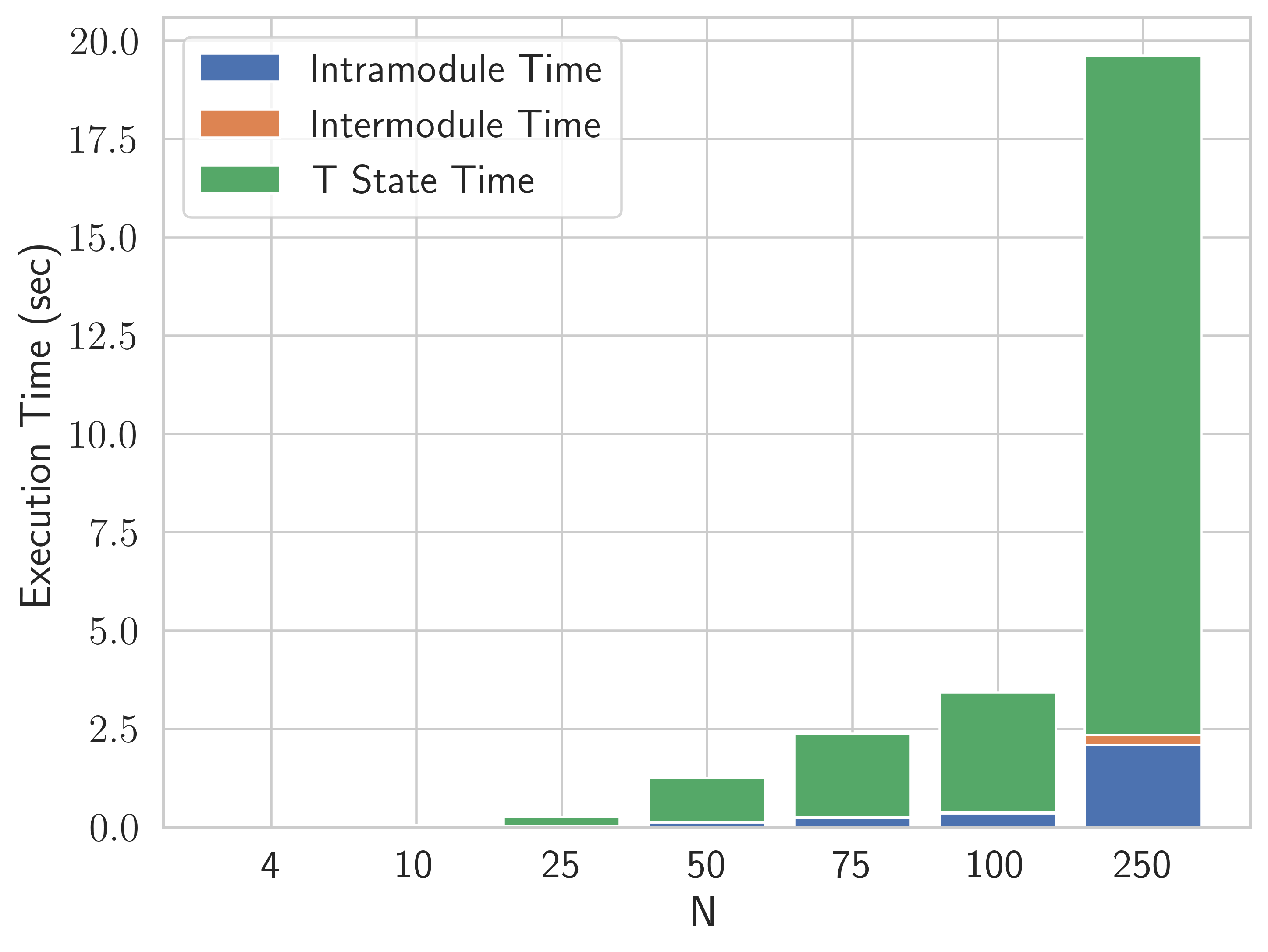
The Quantum Fourier Transform (QFT) is a common component of quantum algorithms, including Quantum Phase Estimation. From the perspective of hardware-specific resource analysis, QFTs are likely to feature in application-relevant resource analysis, yet can be scaled down to a small handful of logical input gates, allowing us to trace and debug compilation workflows in our tool chain at the level of logical operations. The method for generating a Quantum Fourier Transform is based on [58]. This makes QFT circuits ideally suited as first test cases of our estimation framework. In this work we analyze QFT circuits on qubits where or .
II.3 Hamiltonian simulation
Simulation of lattice-based Hamiltonians covers a family of important applications investigated by researchers in quantum chemistry and condensed matter. Moreover, simulating dynamics may provide utility for smaller hardware system sizes than methods for evaluating static properties such as the ground state.
Hamiltonian simulation consists of evolving an initial state to a state at time , according to,
| (21) |
where is the Hamiltonian of the system of interest.
We consider simulation of two families of Hamiltonians; 2D Transverse-Ising models and 2D Fermi-Hubbard models. Each of these will be described in more detail below.
II.3.1 Transverse-Ising Hamiltonian Simulation
The Los Alamos National Laboratory (LANL) has created a public repository containing circuit generation and analysis of problems that may be amenable to quantum computing, and ostensibly are of interest to the scientific community, [59]. Drawing inspiration from their investigation of magnetic lattices, we perform resource estimation for simulation of a time-invariant Transverse-Ising Hamiltonian,
| (22) |
on a triangular lattice, shown in Figure 8.

Here, and and represent the Pauli X and Z operators, respectively, acting on lattice site i, and angle brackets denote lattice sites connected by an edge.
Based on the studies documented by LANL, we carried out resource estimates of simulation of the Hamiltonian in eq. 22 for total time of on a 2D triangular lattice of size where is an integer between and .
II.3.2 Fermi-Hubbard Hamiltonian simulations
We also investigated Fermi-Hubbard simulation as a core computational capability towards solving problems related to room temperature superconductivity. These problems typically involve studying the ground state energy, state configurations, and other observable properties of the system, including time-dependent quantities.
The Fermi-Hubbard Hamiltonian we consider is given by,
| (23) |
where single and double angled brackets denote all nearest neighbor and next-nearest-neighbor lattice site pairs respectively. ) creation (annihilation) operators of a spin- Fermion on the jth lattice site where . (primed or unprimed) and capture the magnitudes of the hopping and repulsion energies respectively. is the number operator, is an external applied magnetic field, and is the chemical potential.
To motivate the specific Fermi-Hubbard simulations we will obtain resource estimates for, we consult the literature to understand configurations that are of interest to the community. Broadly speaking, methods for simulating a Fermi-Hubbard system can be broken into two families; stochastic and deterministic. As mentioned in [60], deterministic methods do not “suffer from numerical issues seen in stochastic simulations when dealing with systems with non-zero chemical potential”. More over this instability due to the “sign problem” becomes prohibitive for moderate . This suggests separating instances into those with , and those with greater than .
Here we reference a few exemplar studies in the literature for both stochastic and deterministic methods.
Some examples of stochastic studies include a study using Auxiliary-field quantum Monte Carlo (AFQMC) to perform ground state estimation on lattice sizes of to and , . [61]. In addition, [62] used Determinant Quantum Monte Carlo (DQMC) to study doped ground state estimation using , , and lattice sizes of , , , . In contrast, examples of deterministic studies included work on numerical linked cluster expansions [63]. In this particular study, researchers selected random repulsion strengths from an uncertainty "box" about . Simulations were for a periodic lattice with , . Others researchers used Projected Density Matrix Embedding (PDME) to perform a 2D Fermi-Hubbard study with , on a lattice [64]. Finally, in [60] the authors use Projected Entangled Pair States (PEPS) with a bond dimension of , and claim that accuracy increases with . Most of their results are from a honeycomb lattice with and , but the authors were able to calculate the ground state via imaginary time evolution on a bipartite honeycomb lattice.
Of note is that in [60] it was determined that the time required to run these studies on a CPU varies like,
where is the truncated bond dimension and the problem dimension. Memory scaled as,
The authors of the study empirically found was sufficiently accurate for their studies, with error about . These estimates provide an interesting guidepost for the tipping point at which FTQCs quantum computers may outperform classical computers for these types of problems.
Taking these studies as examples of the types of systems of interest to the community it suggests obtaining resource estimates for Fermi-Hubbard Hamiltonian simulations consisting of a 2D square lattice for total time , with , , , , , and lattice sides of length .
II.3.3 Algorithm and Approach
Owing to its optimal scaling characteristics, in terms of queries to the block encoding of the Hamiltonian [10], we have chosen Quantum Signal Processing (QSP) as the Hamiltonian simulation algorithm for which we obtain resource estimate for. QSP is briefly described below, but more details can be found in [10], [65], [66], and [67].
Given a Hamiltonian and simulation time , QSP involves performing a sequence of single qubit rotations, parameterized by a sequence of phase angles, interlaced with a quantum walk-like operator. This allows one to apply a polynomial approximation of to the input target state. The sequence of phase angles are responsible for the polynomial approximation, and are computed classically offline, according to the error tolerance of the approximation error desired, captured by the user defined parameter . is also inversely related to the probability of success of the QSP algorithm. Thus, for an accurate simulation, with a high probability of success, may have to be set quite small.
For implementation details, we follow the examples accompanying the pyLIQTR [68] package (v0.3.1), as well as the work done in [69, 70].
For demonstration purposes, we set the desired probability of success of our algorithm, , to be equal to 0.95. In real world applications this is typically fixed to meet outcome requirements (such as accuracy, wall clock time, etc). Denoting the probability of success of a QSP circuit, , we therfore require,
| (24) |
Since circuit size is inversely related to , it is prudent to choose to be as large as possible while still guaranteeing that exceeds the algorithm target of 0.95. According to [10] . Thus, to ensure eq. 24 is satisfied we set,
| (25) |
and so in this work we choose to be equal to 0.025.
II.4 Circuit Synthesis
For our Hamiltonian simulation circuits we used pyLIQTR v0.3.1 to construct the Hamiltonians and synthesize the QSP circuits. The pyLIQTR package provides tools that constructs the Hamiltonians, calculates the necessary phase angles for QSP simulation, and generates QSP circuits. In addition, pyLIQTR also allows the user to request random phase angles rather than solving for the precise values required for an accurate simulation. In our work we used random phase angles. This is appropriate due to the fact that we are only performing resource estimation, and not numerically accurate simulations. The correct number of phase angles is used in the circuits, but their numerical values are random. This maintains the accuracy of the resource estimations without incurring the time consuming step of solving for the phase angles explicitly.
It is worth noting that the version of pyLIQTR we used, v0.3.1, calculates the required QSP angles and gates from a list of coefficient/Pauli string pairs representing the Hamiltonian of interest and also provides some helper methods that create these coefficient/Pauli string pairs for common Hamiltonians. However, Hamiltonian terms involving Fermionic creation and annihilation operators, like those in our Fermi-Hubbard test cases, must be first converted to coefficient/Pauli string pairs before use in pyLIQTR. There are a few different ways to map Fermionic operators to Pauli strings. The most common of these is the Jordan-Wigner Transformation [71, 72], the Bravyi–Kitaev Transformation [73, 74, 75], and the Parity Transformation. Though perhaps inefficient, we chose to use the Jordan-Wigner Transformation due to its simplicity, ease of implementation, and the fact that pyLIQTR v0.3.1 does not exploit potential efficiencies in other transformations anyway.
III Resource estimation results
table 2 summarizes the key physical resource requirements for the test cases described in section II over various input sizes. We demonstrate our tool is capable of estimating resources for problem sizes consistent with studies in the literature, but also reveal where the bottlenecks are to help guide future research.
When we visualize this ensemble of compiled logical resources, and physical resource requirements (fig. 9 and fig. 10 respectively), we seetrajectories that show an increasing trend in resources with increasing problem size. This provides us with some validation of the reasonableness of our methodology, and its benefit as a tool to support studies into the future.
Our methodology allows us to extend the state of the art in a few ways. (1) A full accounting for resources for both T counts, but also for executing the Clifford portions of the circuit as well. (2) A breakdown of physical and temporal resources allocated to portions of the execution of the algorithm, namely: Clifford, T-state and teleportation between modules. (3) A quantitative estimation of the impact on total resources of the performance of subsystems.
The full accounting of both Clifford and T contributions to total resources, (1), is shown in fig. 12 for all families of applications for which we estimated resources. It is interesting to note, that conventional T-counting methodologies don’t often surface the competition for resources between the Clifford and T functions of a quantum architecture. As problems scale, physical qubits need to be allocated to the increased needs of Clifford processing, squeezing out available qubits that could be allocated to magic state distillation. This in turn reduces the number magic state distillation factories that can be applied to a calculation and thus increases runtime in a non-linear fashion.
This impact on the breakdown of total runtime, (2), can be seen in fig. 13. Here the contribution to runtime of magic state distillation increases dramatically for the largest applications considered. This is because fewer qubits are allocated to the creation of higher precision T-states, doubling the penalty in runtime. The impact of runtime on the teleportation present in the distributed architecture can also be seen in this figure. Here, despite a relatively slow inter module interaction time (5x slower than the native code cycle) the contribution to overall runtime is minor for all applications estimated. This shows that for certain architectures, fault tolerance algorithms can be partitioned in a way to allow distributed computing, with relatively low impact.
Moreover, we can test the sensitivity of runtime to parameters in this architectural model, (3). In fig. 11 we select an instance from each family, vary the number of inter-module connections and we calculate the impact to runtime. We define this in terms of a pipe where the number of connections is equal to the required code distance for the algorithm. Additional pipes will allow the teleportation of nodes between widgets to happen in parallel. This is done to quantify the penalty being paid for not having a fully connected lattice of qubits between modules. Here we see that while there is indeed a increased runtime for a reduced number of inter-module connections, there are diminishing returns for approaching addition additional connections and connections with a single connection only have runtime of 10% more in the worst case.
| Input circuit | Graph State Resources | Superconducting FTQC resources | |||
| Instance | logical qubits | Compiled logical qubits | Physical qubits | ||
| Fermi Hubbard | |||||
| 2x2 | 19 | 171 | 1.84M | 2.81s | 0.45kWh |
| 3x3 | 33 | 211 | 1.77M | 27.5s | 4.49kWh |
| 4x4 | 49 | 257 | 1.76M | 1.97m | 19.3kWh |
| 5x5 | 67 | 308 | 1.81M | 7.44m | 73.0kWh |
| 6x6 | 91 | 376 | 1.91M | 21.3m | 209kWh |
| 7x7 | 117 | 456 | 1.70M | 51.9m | 509kWh |
| 8x8 | 149 | 562 | 1.60M | 151m | 1.48MWh |
| QFT | |||||
| N-4 | 4 | 27 | 1.93M | 769s | 0.13Wh |
| N-10 | 10 | 89 | 1.66M | 53.8ms | 8.80Wh |
| N-25 | 25 | 339 | 1.81M | 258ms | 42.2Wh |
| N-50 | 50 | 544 | 1.87M | 1.25s | 205Wh |
| N-75 | 75 | 569 | 1.83M | 2.38s | 389Wh |
| N-100 | 100 | 594 | 1.86M | 3.42s | 560Wh |
| N-250 | 250 | 809 | 1.72M | 19.6s | 3.21kWh |
| Transverse-Ising | |||||
| 2x2 | 13 | 175 | 1.68M | 145ms | 23.7Wh |
| 3x3 | 20 | 203 | 1.76M | 1.20s | 197Wh |
| 4x4 | 29 | 246 | 1.85M | 5.08s | 831Wh |
| 5x5 | 40 | 291 | 1.72M | 20.2s | 3.30kWh |
| 6x6 | 51 | 285 | 1.71M | 38.5s | 6.29kWh |
| 7x7 | 66 | 326 | 1.77M | 1.73m | 16.9kWh |
| 8x8 | 81 | 365 | 1.89M | 4.47m | 44.0kWh |
| 9x9 | 100 | 458 | 1.89M | 11.0m | 108kWh |
| 10x10 | 119 | 491 | 1.80M | 16.8m | 164kWh |


IV Future Work
The results from Section III can be improved by focusing on at least the following two aspects: a) using a decoder which is faster and/or has better scaling than the standard choice of minimum weight perfect matching (MPWM); b) optimizing the widget circuits by, for example, reducing circuit gate counts and depths. The savings potential of these two approaches will be detailed in the following.
IV.1 Replacing the MWPM decoder
The minimum weight perfect matching decoder is the de facto decoder for performing resource estimates. Other decoders have been proposed, but MWPM is still the most efficient when it comes to the decoding speed vs. physical error rate trade off: MWPM can handle high error-rates while it’s complexity is polynomial. There are faster, lower polynomial complexity decoders (e.g. union-find variations, or pure belief-propagation), and decoders with linear complexity, but which are difficult to scale to high distances (machine learning decoders).
Although better or faster alternatives to MWPM exist, to the best of our knowledge, there existed no alternative decoder that has, at the same time, a lower degree polynomial decoding complexity and a threshold higher than MWPM.
Herein, we report preliminary results (Figure 14) about a machine learning decoder that outperforms MWPM: it has a higher threshold and it has also a linear complexity. Our machine learning decoder uses graph neural networks (GNNs) in a novel way: we are learning a message passing algorithm on the Tanner graph of the codes. Currently we are able to train, within hours, such decoders with gaming GPUs for surface codes up to distance 11. In contrast to other machine learning decoders, the training time of our decoder is significantly lower (e.g. [76]) for comparable depths.


We train distinct GNN decoders for each distance using syndromes collected by passing the surface codes through a code capacity noise channel. This channel assumes that the data qubits are affected by noise with a probability and that the syndrome measurements are perfect. For the purpose of this work, we do not report the decoding of circuit level correlated noise (e.g. [77]) and focus entirely on the correction of depolarizing noise.
After training our decoders, we evaluate numerically their decoding performance and capture the decoder’s performance through an equation of the type from Eq. 28
| (26) |
Usually the performance scaling equations for the surface code are obtained by simulations with circuit level noise (e.g. Eq. 28), because this is considered to be the most exact model. Nevertheless, for benchmarking the preliminary versions of a decoder, the code capacity is more straightforward to implement. In order to allow the comparison between MWPM and GNN, we benchmark MWPM with code capacity noise, too. The results are illustrated in Fig. 14. Based on the MWPM code capacity errors, we obtain the MWPM scaling equation:
| (27) |
By comparing, with one can observe that the GNN has a higher threshold () and offers faster (better) logical error suppression (). This implies, that the same logical error-rate can be achieved with lower distance surface codes by simply replacing the MWPM with the GNN decoder. Future work will focus on quantify the exact savings when utilizing our decoder, after benchmarking its performance under circuit level noise.
IV.2 Ultra-large scale circuit optimization
The Fermi-Hubbard circuit instances analyzed in the previous sections are, for practical regimes, too large in terms of gate counts. Compiling, analyzing and optimizing such circuits at graph-state or Clifford+T level is challenging: the state-of-the-art quantum software tools are not able to handle ultra-large-scale circuits.
Widgets (Section A.7) are subcircuits representing relevant parts of the larger circuits. Due to their size, widgets can be more easily analyzed and optimized. Nevertheless, even widgets are extremely difficult to optimize for metrics such as T-count, T-depth. Optimization is a highly complex task and most optimization heuristics are not designed (or do not perform as expected) for (sub)circuits of tens of qubits and hundreds of gates.
Tools like pyLQTR are built on top of other quantum software frameworks, such as Google Cirq, which were not designed for extreme scalability. We bridge this gap by designing and implementing a software tool that can easily handle ultra-large scale circuits. Our tool is based on PostgreSQL and leverages the capabilities of modern relational database software. Our tool is also supporting multi-threaded operations on quantum circuits.
Table 3 reports preliminary results on the optimization of arithmetic widgets as presented in [78]. The latter are very common building blocks of practical application circuits such as Fermi-Hubbard. Our optimization procedure for optimizing the circuits is not as complex as the one described by Ref. [78]. We implemented a heuristic that uses multiple threads for applying circuit template rewrites [78]:
-
•
decomposition of gates (e.g. Toffoli);
-
•
cancelling H, T, X gates;
-
•
cancelling CNOT gates;
-
•
commuting gates to the left and to the right;
-
•
reversing directions of CNOT gates.
Our software offers a simple API which can be used to develop new and more complex optimization methods. We interfaced our tool with Google Qualtran and can easily extract extremely large circuits for analysis and optimization. Currently, the circuits and widgets available in Qualtran have been optimized manually such that automatic optimization is even more challenging. Therefore, the results from Table 3 are for circuits known to be far from optimal.
To conclude, quantum software for ultra-large-scale circuit analysis and optimization has the potential to lower the resources required for practical quantum computing applications. Our tool is a first step towards optimizing at scale.
| Circuit | Orig. T-count | Opt. T-count | Impr. |
|---|---|---|---|
| Adder8 | 266 | 236 | 11.27% |
| Adder16 | 602 | 536 | 10.96% |
| Adder32 | 1274 | 1144 | 10.20% |
| Adder64 | 2618 | 2368 | 9.54% |
| Adder128 | 5306 | 4648 | 11.64% |
| Adder256 | 10682 | 9258 | 13.33% |
| Adder512 | 21434 | 18562 | 13.39% |
| Adder1024 | 42938 | 38216 | 10.99% |
| Adder2048 | 85946 | 76056 | 11.50% |
V Conclusion
In this paper, we have described a resource estimation framework and software tool that estimates the physical resources needed for quantum algorithms and presented estimates for test cases based on the literature. We have shown that a fault-tolerant quantum computer based on on a distributed superconducting architecture, consisting of two modules could, in principle, house 2,000,000 physical qubits and could serve scientifically interesting applications in a reasonable run-time. These estimates are consistent in their trajectory to established results such as factoring. This model-driven approach provides specificity in how a superconducting platform could achieve such a feat, including descriptions of scheduled execution over the preparation and consumption of graph-states and hardware-level justifications for some of the most important size, weight, and power considerations.
This work has also enables research towards assuring that real quantum computing platforms can be engineered to provide the espoused benefits of fault-tolerant operation. This includes addressing issues such as very low error rate T-state distillation widgets, but more broadly provides a software test-bed for evaluating the impact of algorithmic, compilation, decoding, and physical-layer intrinsic or system architecture proposals. Rapid iteration in a simulated space is a proven methodology for accelerating technology growth, and we hope that our efforts in producing this tooling contribute positively to this endeavor.
VI Acknowledgements
The views, opinions and/or findings expressed are those of the author(s) and should not be interpreted as representing the official views or policies of the Department of Defense or the U.S. Government. This research was developed with funding from the Defense Advanced Research Projects Agency under Agreement HR00112230006. Jannis Ruh was supported by the Sydney Quantum Academy, Sydney, NSW, Australia.
References
- Campbell et al. [2017] E. T. Campbell, B. M. Terhal, and C. Vuillot, Roads towards fault-tolerant universal quantum computation, Nature 549, 172 (2017).
- Webster et al. [2022] P. Webster, M. Vasmer, T. R. Scruby, and S. D. Bartlett, Universal fault-tolerant quantum computing with stabilizer codes, Phys. Rev. Res. 4, 013092 (2022).
- Acharya et al. [2023] R. Acharya, I. Aleiner, R. Allen, T. I. Andersen, M. Ansmann, F. Arute, K. Arya, A. Asfaw, J. Atalaya, R. Babbush, D. Bacon, J. C. Bardin, J. Basso, A. Bengtsson, S. Boixo, G. Bortoli, A. Bourassa, J. Bovaird, L. Brill, M. Broughton, B. B. Buckley, D. A. Buell, T. Burger, B. Burkett, N. Bushnell, Y. Chen, Z. Chen, B. Chiaro, J. Cogan, R. Collins, P. Conner, W. Courtney, A. L. Crook, B. Curtin, D. M. Debroy, A. Del Toro Barba, S. Demura, A. Dunsworth, D. Eppens, C. Erickson, L. Faoro, E. Farhi, R. Fatemi, L. Flores Burgos, E. Forati, A. G. Fowler, B. Foxen, W. Giang, C. Gidney, D. Gilboa, M. Giustina, A. Grajales Dau, J. A. Gross, S. Habegger, M. C. Hamilton, M. P. Harrigan, S. D. Harrington, O. Higgott, J. Hilton, M. Hoffmann, S. Hong, T. Huang, A. Huff, W. J. Huggins, L. B. Ioffe, S. V. Isakov, J. Iveland, E. Jeffrey, Z. Jiang, C. Jones, P. Juhas, D. Kafri, K. Kechedzhi, J. Kelly, T. Khattar, M. Khezri, M. Kieferová, S. Kim, A. Kitaev, P. V. Klimov, A. R. Klots, A. N. Korotkov, F. Kostritsa, J. M. Kreikebaum, D. Landhuis, P. Laptev, K.-M. Lau, L. Laws, J. Lee, K. Lee, B. J. Lester, A. Lill, W. Liu, A. Locharla, E. Lucero, F. D. Malone, J. Marshall, O. Martin, J. R. McClean, T. McCourt, M. McEwen, A. Megrant, B. Meurer Costa, X. Mi, K. C. Miao, M. Mohseni, S. Montazeri, A. Morvan, E. Mount, W. Mruczkiewicz, O. Naaman, M. Neeley, C. Neill, A. Nersisyan, H. Neven, M. Newman, J. H. Ng, A. Nguyen, M. Nguyen, M. Y. Niu, T. E. O’Brien, A. Opremcak, J. Platt, A. Petukhov, R. Potter, L. P. Pryadko, C. Quintana, P. Roushan, N. C. Rubin, N. Saei, D. Sank, K. Sankaragomathi, K. J. Satzinger, H. F. Schurkus, C. Schuster, M. J. Shearn, A. Shorter, V. Shvarts, J. Skruzny, V. Smelyanskiy, W. C. Smith, G. Sterling, D. Strain, M. Szalay, A. Torres, G. Vidal, B. Villalonga, C. Vollgraff Heidweiller, T. White, C. Xing, Z. J. Yao, P. Yeh, J. Yoo, G. Young, A. Zalcman, Y. Zhang, N. Zhu, and G. Q. AI, Suppressing quantum errors by scaling a surface code logical qubit, Nature 614, 676 (2023).
- de Leon et al. [2021] N. P. de Leon, K. M. Itoh, D. Kim, K. K. Mehta, T. E. Northup, H. Paik, B. S. Palmer, N. Samarth, S. Sangtawesin, and D. W. Steuerman, Materials challenges and opportunities for quantum computing hardware, Science 372, eabb2823 (2021), https://www.science.org/doi/pdf/10.1126/science.abb2823 .
- Field et al. [2023] M. Field, A. Q. Chen, B. Scharmann, E. A. Sete, F. Oruc, K. Vu, V. Kosenko, J. Y. Mutus, S. Poletto, and A. Bestwick, Modular superconducting qubit architecture with a multi-chip tunable coupler (2023), arXiv:2308.09240 [quant-ph] .
- Fowler et al. [2012] A. G. Fowler, M. Mariantoni, J. M. Martinis, and A. N. Cleland, Surface codes: Towards practical large-scale quantum computation, Phys. Rev. A 86, 032324 (2012).
- Litinski [2019a] D. Litinski, A Game of Surface Codes: Large-Scale Quantum Computing with Lattice Surgery, Quantum 3, 128 (2019a).
- Üstün et al. [2024] G. Üstün, A. Morello, and S. Devitt, Single-step parity check gate set for quantum error correction, Quantum Science and Technology 9, 035037 (2024).
- Gidney and Ekerå [2021] C. Gidney and M. Ekerå, How to factor 2048 bit rsa integers in 8 hours using 20 million noisy qubits, Quantum 5, 433 (2021).
- Low and Chuang [2017] G. H. Low and I. L. Chuang, Optimal hamiltonian simulation by quantum signal processing, Physical review letters 118, 010501 (2017).
- Lin and Tong [2022] L. Lin and Y. Tong, Heisenberg-limited ground-state energy estimation for early fault-tolerant quantum computers, PRX Quantum 3, 010318 (2022).
- Litinski [2019b] D. Litinski, A game of surface codes: Large-Scale quantum computing with lattice surgery, Quantum 3, 128 (2019b).
- Paler and Fowler [2019] A. Paler and A. G. Fowler, Opensurgery for topological assemblies, arXiv preprint arXiv:1906.07994 (2019).
- [14] A. Nguyen, G. Watkins, K. Watkins, and V. Seshadri, lattice-surgery-compiler, accessed June 10, 2024.
- Beverland et al. [2022] M. E. Beverland, P. Murali, M. Troyer, K. M. Svore, T. Hoefler, V. Kliuchnikov, G. H. Low, M. Soeken, A. Sundaram, and A. Vaschillo, Assessing requirements to scale to practical quantum advantage (2022), arXiv:2211.07629 [quant-ph] .
- [16] Microsoft azure quantum resource estimation, accessed June 10, 2024.
- Hein et al. [2004] M. Hein, J. Eisert, and H. J. Briegel, Multiparty entanglement in graph states, Physical Review A 69, 062311 (2004).
- Anders and Briegel [2006] S. Anders and H. J. Briegel, Fast simulation of stabilizer circuits using a graph-state representation, Physical Review A 73, 022334 (2006).
- Vijayan et al. [2024] M. K. Vijayan, A. Paler, J. Gavriel, C. R. Myers, P. P. Rohde, and S. J. Devitt, Compilation of algorithm-specific graph states for quantum circuits, Quantum Science and Technology 9, 025005 (2024).
- Raussendorf and Briegel [2001a] R. Raussendorf and H. J. Briegel, A one-way quantum computer, Phys. Rev. Lett. 86, 5188 (2001a).
- Raussendorf and Briegel [2001b] R. Raussendorf and H. Briegel, Computational model underlying the one-way quantum computer, arXiv preprint quant-ph/0108067 (2001b).
- Raussendorf et al. [2003] R. Raussendorf, D. E. Browne, and H. J. Briegel, Measurement-based quantum computation on cluster states, Physical review A 68, 022312 (2003).
- Nielsen [2006] M. A. Nielsen, Cluster-state quantum computation, Reports on Mathematical Physics 57, 147 (2006).
- Paler et al. [2017] A. Paler, I. Polian, K. Nemoto, and S. J. Devitt, Fault-tolerant, high-level quantum circuits: form, compilation and description, Quantum Science and Technology 2, 025003 (2017).
- Vijayan [2024] M. e. a. Vijayan, Modular compilation and resource computation based on graph states, In Preparation (2024).
- Ruh and Devitt [2024] J. Ruh and S. Devitt, Quantum circuit optimisation and mbqc scheduling with a pauli tracking library, arXiv:2405.03970 (2024).
- Elman et al. [2024] S. Elman, J. Gavriel, and R. Mann, Optimal scheduling of graph states via path decompositions, arXiv:2403.04126 (2024).
- Ross and Selinger [2014] N. J. Ross and P. Selinger, Optimal ancilla-free clifford+t approximation of z-rotations 10.48550/ARXIV.1403.2975 (2014).
- Kliuchnikov et al. [2022] V. Kliuchnikov, K. Lauter, R. Minko, A. Paetznick, and C. Petit, Shorter quantum circuits (2022).
- [30] M. K. Vijayan, S. Devitt, P. Rohde, A. Paler, C. Mayers, J. Gavriel, M. Stęchły, S. Jones, and A. Caesura, Jabalizer, accessed June 10, 2024.
- [31] Aqua, Substrate scheduler, graph-state-generation, accessed June 10, 2024.
- Litinski [2019c] D. Litinski, Magic State Distillation: Not as Costly as You Think, Quantum 3, 205 (2019c).
- Devitt et al. [2014] S. J. Devitt, A. D. Greentree, A. M. Stephens, and R. Van Meter, High-speed quantum networking by ship, arXiv e-prints , arXiv:1410.3224 (2014), arXiv:1410.3224 [quant-ph] .
- Chubb [2021] C. T. Chubb, General tensor network decoding of 2d pauli codes (2021).
- Piveteau et al. [2023] C. Piveteau, C. T. Chubb, and J. M. Renes, Tensor network decoding beyond 2d (2023), arXiv:2310.10722 [quant-ph] .
- Yan et al. [2018] F. Yan, P. Krantz, Y. Sung, M. Kjaergaard, D. L. Campbell, T. P. Orlando, S. Gustavsson, and W. D. Oliver, Tunable coupling scheme for implementing high-fidelity two-qubit gates, Physical Review Applied 10, 10.1103/physrevapplied.10.054062 (2018).
- Arute et al. [2019] F. Arute, K. Arya, R. Babbush, D. Bacon, J. Bardin, R. Barends, R. Biswas, S. Boixo, F. Brandao, D. Buell, B. Burkett, Y. Chen, J. Chen, B. Chiaro, R. Collins, W. Courtney, A. Dunsworth, E. Farhi, B. Foxen, A. Fowler, C. M. Gidney, M. Giustina, R. Graff, K. Guerin, S. Habegger, M. Harrigan, M. Hartmann, A. Ho, M. R. Hoffmann, T. Huang, T. Humble, S. Isakov, E. Jeffrey, Z. Jiang, D. Kafri, K. Kechedzhi, J. Kelly, P. Klimov, S. Knysh, A. Korotkov, F. Kostritsa, D. Landhuis, M. Lindmark, E. Lucero, D. Lyakh, S. Mandrà, J. R. McClean, M. McEwen, A. Megrant, X. Mi, K. Michielsen, M. Mohseni, J. Mutus, O. Naaman, M. Neeley, C. Neill, M. Y. Niu, E. Ostby, A. Petukhov, J. Platt, C. Quintana, E. G. Rieffel, P. Roushan, N. Rubin, D. Sank, K. J. Satzinger, V. Smelyanskiy, K. J. Sung, M. Trevithick, A. Vainsencher, B. Villalonga, T. White, Z. J. Yao, P. Yeh, A. Zalcman, H. Neven, and J. Martinis, Quantum supremacy using a programmable superconducting processor, Nature 574, 505–510 (2019).
- Xu et al. [2023] S. Xu, Z.-Z. Sun, K. Wang, L. Xiang, Z. Bao, Z. Zhu, F. Shen, Z. Song, P. Zhang, W. Ren, X. Zhang, H. Dong, J. Deng, J. Chen, Y. Wu, Z. Tan, Y. Gao, F. Jin, X. Zhu, C. Zhang, N. Wang, Y. Zou, J. Zhong, A. Zhang, W. Li, W. Jiang, L.-W. Yu, Y. Yao, Z. Wang, H. Li, Q. Guo, C. Song, H. Wang, and D.-L. Deng, Digital simulation of projective non-abelian anyons with 68 superconducting qubits, Chinese Physics Letters 40, 060301 (2023).
- Wu et al. [2021] Y. Wu, W.-S. Bao, S. Cao, F. Chen, M.-C. Chen, X. Chen, T.-H. Chung, H. Deng, Y. Du, D. Fan, M. Gong, C. Guo, C. Guo, S. Guo, L. Han, L. Hong, H.-L. Huang, Y.-H. Huo, L. Li, N. Li, S. Li, Y. Li, F. Liang, C. Lin, J. Lin, H. Qian, D. Qiao, H. Rong, H. Su, L. Sun, L. Wang, S. Wang, D. Wu, Y. Xu, K. Yan, W. Yang, Y. Yang, Y. Ye, J. Yin, C. Ying, J. Yu, C. Zha, C. Zhang, H. Zhang, K. Zhang, Y. Zhang, H. Zhao, Y. Zhao, L. Zhou, Q. Zhu, C.-Y. Lu, C.-Z. Peng, X. Zhu, and J.-W. Pan, Strong quantum computational advantage using a superconducting quantum processor, Physical Review Letters 127, 10.1103/physrevlett.127.180501 (2021).
- Robledo-Moreno et al. [2024] J. Robledo-Moreno, M. Motta, H. Haas, A. Javadi-Abhari, P. Jurcevic, W. Kirby, S. Martiel, K. Sharma, S. Sharma, T. Shirakawa, I. Sitdikov, R.-Y. Sun, K. J. Sung, M. Takita, M. C. Tran, S. Yunoki, and A. Mezzacapo, Chemistry beyond exact solutions on a quantum-centric supercomputer (2024), arXiv:2405.05068 [quant-ph] .
- Manenti et al. [2021] R. Manenti, E. A. Sete, A. Q. Chen, S. Kulshreshtha, J.-H. Yeh, F. Oruc, A. Bestwick, M. Field, K. Jackson, and S. Poletto, Full control of superconducting qubits with combined on-chip microwave and flux lines, Applied Physics Letters 119 (2021).
- Sank et al. [2024] D. Sank, A. Opremcak, A. Bengtsson, M. Khezri, Z. Chen, O. Naaman, and A. Korotkov, System characterization of dispersive readout in superconducting qubits (2024), arXiv:2402.00413 [quant-ph] .
- Mallek et al. [2021] J. L. Mallek, D.-R. W. Yost, D. Rosenberg, J. L. Yoder, G. Calusine, M. Cook, R. Das, A. Day, E. Golden, D. K. Kim, J. Knecht, B. M. Niedzielski, M. Schwartz, A. Sevi, C. Stull, W. Woods, A. J. Kerman, and W. D. Oliver, Fabrication of superconducting through-silicon vias (2021), arXiv:2103.08536 [quant-ph] .
- Rosenberg et al. [2017] D. Rosenberg, D. Kim, R. Das, D. Yost, S. Gustavsson, D. Hover, P. Krantz, A. Melville, L. Racz, G. O. Samach, S. J. Weber, F. Yan, J. L. Yoder, A. J. Kerman, and W. D. Oliver, 3d integrated superconducting qubits, npj Quantum Information 3, 10.1038/s41534-017-0044-0 (2017).
- Martinis and Osborne [2004] J. M. Martinis and K. Osborne, Superconducting qubits and the physics of josephson junctions (2004), arXiv:cond-mat/0402415 [cond-mat.supr-con] .
- Kreikebaum et al. [2020] J. M. Kreikebaum, K. P. O’Brien, A. Morvan, and I. Siddiqi, Improving wafer-scale josephson junction resistance variation in superconducting quantum coherent circuits, Superconductor Science and Technology 33, 06LT02 (2020).
- Pappas et al. [2024] D. P. Pappas, M. Field, C. Kopas, J. A. Howard, X. Wang, E. Lachman, L. Zhou, J. Oh, K. Yadavalli, E. A. Sete, A. Bestwick, M. J. Kramer, and J. Y. Mutus, Alternating bias assisted annealing of amorphous oxide tunnel junctions (2024), arXiv:2401.07415 [physics.app-ph] .
- Damme et al. [2024] J. V. Damme, S. Massar, R. Acharya, T. Ivanov, D. P. Lozano, Y. Canvel, M. Demarets, D. Vangoidsenhoven, Y. Hermans, J.-G. Lai, V. Rao, M. Mongillo, D. Wan, J. D. Boeck, A. Potocnik, and K. D. Greve, High-coherence superconducting qubits made using industry-standard, advanced semiconductor manufacturing (2024), arXiv:2403.01312 [quant-ph] .
- Sete et al. [2021] E. A. Sete, A. Q. Chen, R. Manenti, S. Kulshreshtha, and S. Poletto, Floating tunable coupler for scalable quantum computing architectures, Physical Review Applied 15, 064063 (2021).
- Smith et al. [2022] K. N. Smith, G. S. Ravi, J. M. Baker, and F. T. Chong, Scaling superconducting quantum computers with chiplet architectures (2022), arXiv:2210.10921 [quant-ph] .
- McEwen et al. [2023] M. McEwen, D. Bacon, and C. Gidney, Relaxing hardware requirements for surface code circuits using time-dynamics, arXiv preprint arXiv:2302.02192 (2023).
- Gidney [2023a] C. Gidney, midout, https://github.com/Strilanc/midout (2023a).
- Gidney [2021] C. Gidney, Stim: a fast stabilizer circuit simulator, Quantum 5, 497 (2021).
- Higgott [2022] O. Higgott, Pymatching: A python package for decoding quantum codes with minimum-weight perfect matching, ACM Transactions on Quantum Computing 3, 1 (2022).
- Chu and Yan [2021] J. Chu and F. Yan, Coupler-assisted controlled-phase gate with enhanced adiabaticity, Physical Review Applied 16, 054020 (2021).
- [56] S. Krinner, S. Storz, P. Kurpiers, P. Magnard, J. Heinsoo, R. Keller, J. Lütolf, C. Eichler, and A. Wallraff, Engineering cryogenic setups for 100-qubit scale superconducting circuit systems, EPJ Quantum Technology 6, 10.1140/epjqt/s40507-019-0072-0.
- Martinez et al. [2010] A. Martinez, A. L. Klebaner, J. C. Theilacker, B. D. DeGraff, J. Leibfritz, and J. G. Weisend, DESIGN AND TESTING OF THE NEW MUON LAB CRYOGENIC SYSTEM AT FERMILAB, in AIP Conference Proceedings (AIP, 2010).
- Nielsen and Chuang [2010] M. A. Nielsen and I. L. Chuang, Quantum Computation and Quantum Information: 10th Anniversary Edition (Cambridge University Press, 2010).
- LAN [2024] qc-applications, https://github.com/lanl-ansi/qc-applications/ (2024).
- Schneider et al. [2021] M. Schneider, J. Ostmeyer, K. Jansen, T. Luu, and C. Urbach, Simulating both parity sectors of the hubbard model with tensor networks, Physical Review B 104, 155118 (2021).
- Qin et al. [2016] M. Qin, H. Shi, and S. Zhang, Benchmark study of the two-dimensional hubbard model with auxiliary-field quantum monte carlo method, Physical Review B 94, 085103 (2016).
- Huang et al. [2019] E. W. Huang, R. Sheppard, B. Moritz, and T. P. Devereaux, Strange metallicity in the doped hubbard model, Science 366, 987 (2019).
- Park and Khatami [2021] J. Park and E. Khatami, Thermodynamics of the disordered hubbard model studied via numerical linked-cluster expansions, Physical Review B 104, 165102 (2021).
- Wu et al. [2019] X. Wu, Z.-H. Cui, Y. Tong, M. Lindsey, G. K.-L. Chan, and L. Lin, Projected density matrix embedding theory with applications to the two-dimensional hubbard model, The Journal of Chemical Physics 151, 064108 (2019).
- Low and Chuang [2019] G. H. Low and I. L. Chuang, Hamiltonian simulation by qubitization, Quantum 3, 163 (2019).
- Martyn et al. [2021] J. M. Martyn, Z. M. Rossi, A. K. Tan, and I. L. Chuang, Grand unification of quantum algorithms, PRX Quantum 2, 040203 (2021).
- Dalzell et al. [2023] A. M. Dalzell, S. McArdle, M. Berta, P. Bienias, C.-F. Chen, A. Gilyén, C. T. Hann, M. J. Kastoryano, E. T. Khabiboulline, A. Kubica, et al., Quantum algorithms: A survey of applications and end-to-end complexities, arXiv preprint arXiv:2310.03011 (2023).
- [68] K. Obenland, J. Elenewski, K. Morrell, R. S. Neumann, A. Kurlej, R. Rood, J. Blue, J. Belarge, B. Rempfer, and P. Kuklinski, pyliqtr, accessed June 10, 2024.
- Martyn et al. [2023] J. M. Martyn, Y. Liu, Z. E. Chin, and I. L. Chuang, Efficient fully-coherent quantum signal processing algorithms for real-time dynamics simulation, The Journal of Chemical Physics 158, 024106 (2023).
- Zeytinoğlu and Sugiura [2022] S. Zeytinoğlu and S. Sugiura, Error-robust quantum signal processing using rydberg atoms, (2022), arXiv:2201.04665 [quant-ph] .
- Jordan and Wigner [1993] P. Jordan and E. P. Wigner, Über das paulische äquivalenzverbot (Springer, 1993).
- Aspuru-Guzik et al. [2005] A. Aspuru-Guzik, A. D. Dutoi, P. J. Love, and M. Head-Gordon, Simulated quantum computation of molecular energies, Science 309, 1704 (2005).
- Bravyi and Kitaev [2002] S. B. Bravyi and A. Y. Kitaev, Fermionic quantum computation, Annals of Physics 298, 210 (2002).
- Seeley et al. [2012] J. T. Seeley, M. J. Richard, and P. J. Love, The bravyi-kitaev transformation for quantum computation of electronic structure, The Journal of chemical physics 137 (2012).
- Tranter et al. [2015] A. Tranter, S. Sofia, J. Seeley, M. Kaicher, J. McClean, R. Babbush, P. V. Coveney, F. Mintert, F. Wilhelm, and P. J. Love, The b ravyi–k itaev transformation: Properties and applications, International Journal of Quantum Chemistry 115, 1431 (2015).
- Varsamopoulos et al. [2019] S. Varsamopoulos, K. Bertels, and C. G. Almudever, Comparing neural network based decoders for the surface code, IEEE Transactions on Computers 69, 300 (2019).
- Paler and Fowler [2023] A. Paler and A. G. Fowler, Pipelined correlated minimum weight perfect matching of the surface code, Quantum 7, 1205 (2023).
- Nam et al. [2018] Y. Nam, N. J. Ross, Y. Su, A. M. Childs, and D. Maslov, Automated optimization of large quantum circuits with continuous parameters, npj Quantum Information 4, 23 (2018).
- Pauli-Tracker contributors [2024] Pauli-Tracker contributors, Pauli tracker: A library to track Pauli gates through Clifford circuits (2024), avalaible at https://github.com/taeruh/pauli_tracker.
- mbq [2024] Mbqc scheduling, https://pypi.org/project/mbqc-scheduling/ (2024).
- Gidney [2023b] C. Gidney, sinter, https://pypi.org/project/sinter/ (2023b).
- Virtanen et al. [2020] P. Virtanen, R. Gommers, T. E. Oliphant, M. Haberland, T. Reddy, D. Cournapeau, E. Burovski, P. Peterson, W. Weckesser, J. Bright, S. J. van der Walt, M. Brett, J. Wilson, K. J. Millman, N. Mayorov, A. R. J. Nelson, E. Jones, R. Kern, E. Larson, C. J. Carey, İ. Polat, Y. Feng, E. W. Moore, J. VanderPlas, D. Laxalde, J. Perktold, R. Cimrman, I. Henriksen, E. A. Quintero, C. R. Harris, A. M. Archibald, A. H. Ribeiro, F. Pedregosa, P. van Mulbregt, and SciPy 1.0 Contributors, SciPy 1.0: Fundamental Algorithms for Scientific Computing in Python, Nature Methods 17, 261 (2020).
- Bravyi et al. [2014] S. Bravyi, M. Suchara, and A. Vargo, Efficient algorithms for maximum likelihood decoding in the surface code, Phys. Rev. A 90, 032326 (2014).
Appendix A Supplemental Material
A.1 RRE software pipeline: IOs and configurations
The bi-linear-bus two-fridge architecture of section I.3 and graph-state-based estimation methodology of section V are implemented in Rigetti’s Resource Estimation software (RRE).
In short, the RRE estimation pipeline is centred around a workflow that includes transpiling a logical circuit, mapping it into specific quantum graph states and Pauli frames, then onto a geometric layout of logically-encoded qubits, and finally to the physical resources required. The step-by-step is detailed below with a schematic overview provided in fig. 15.

-
1.
Widgetized JSON and other parameter inputs: The user inputs a widgetized logical algorithm converted from a cirq circuit. The user also needs to input a unified system architectural configuration, , containing important parameters such as the total failure rate budget, , and -to- scaling coefficients. For the presented results in section III, was informed by the decoder and device modeling information detailed in section V. RRE can also accept a standard OpenQASM 2.0 circuit input if no widgetization is desired.
-
2.
Transpilation: We parse the QASM strings, counting initial T and small-angle rotation gates in the logical algorithm as required for later steps, and replace any unitary not supported by downstream compilers in the input using exact gate equivalences.
-
3.
ICM compilation: Jabalizer v0.5.2 [30] is invoked to compile the transpiled subcircuits into .
-
4.
Graph state processing: Pauli Tracker v0.4.1[79] and MBQC Scheduling v0.1.0[80] were invoked to process Jabalizer’s outputs to Pauli corrections, consumption schedule, and other required sets. Each graph object and Pauli frame information are reusable and cached as a .json file. Even if the architecture was altered, this portable graph object could estimate resources for the algorithm, , without requiring further graph state processing. We have used the default configurations for Pauli Tracker and MBQC Scheduling for all reported results, which includes generating the trivial "time-optimal" consumption sub-schedules and initializing all circuits in .
-
5.
Substrate Scheduling: The Substrate Scheduler v0.2.0[31] is invoked to produce a preparation schedule of stabilizer measurements to initialize each (sub)graph states.
-
6.
Find the required precision and code distance iteratively: Given , the graph, and the schedules, loop through a Lookup Widget Table (e.g. table 1), iteratively find , , the most optimum widget that satisfies and . sets the length of the Clifford+ chain, , for arbitrary angle transformations required at the measurement points in the end.
-
7.
Identify space complexity: Find the total physical qubit number that hardware would require, which scales with , the number of required logical qubits provided by Pauli Tracker outputs. See algorithm 1 for details.
-
8.
Identify time complexity: Given and characteristic timescales set in the system architectural configuration, find .
-
9.
Find full PhysResources object and hardware times: Use the tocks, schedule, and other proprietary architectural configurations from the YAML (fridge sizes, line, coupler, power dissipation details, etc.) to fully identify an FT hardware object, PhysResources, including number of couplers, number of inter-modular pipes, areas, memory, energy usage, etc. PhysResources fully identifies all outputs including total FT hardware time, decoding core numbers, and total power and energy consumption. Hardware execution times are calculated based on the intra and inter-modular operations on the ancilla bus. See below for details.
-
10.
Display results: Tabulate and print resource estimation outputs to the console and a CSV file as requested.
To generate the data used to determine the coefficients in Eq. 28, we perform decoder simulations using Stim and Sinter [81]. These simulations use combinations of seven physical error rates and three different code distances for 21 different experiments. For each experiment we simulate the square planar iSWAP error correction circuit for 1 million shots. For each shot, the error correction circuit is repeated times. To fit the parameters we use multivariable least squares fitting implemented in the scipy numerical package [82]. The result of these simulations results in the scaling law,
| (28) |
Next, we list selected configuration parameters we used to generate the results of section III, and, finally, we conclude by providing a glossary of the logical and hardware parameters that RRE outputs by default and were used throughout this paper.
A.1.1 User-inputted system architecture configurations,
As discussed for resource estimations, the user must fix a large set of system parameters in addition to a logical input, . These include but are not limited to physical error rate, cycle times, and the desired total failure rate budget for the QEC process. We collectively refer to these parameters as the system architecture configuration, . RRE users can select pre-configured and edit such parameters as a YAML file. A selection of the configuration parameters we have used for application instances in section III is reported in table 4.
| Parameter | Symbol | Value |
|---|---|---|
| Physical error rate, all quantum ops | 0.001 | |
| Characteristic cycle time, intra quantum ops | 200 ns | |
| Characteristic TN decoding time | 1 ms | |
| No. of inter-modular pipes connecting fridge pairs | 1 | |
| Failure rate budget, full algorithm | 5% |
A.1.2 Glossary of default output parameters
With the workflows of the graph-state estimation methodology and RRE laid out, we can summarize, reiterate, and, in some cases, provide new details on Rigetti’s selected output parameters and how they were formulated. The following are RRE’s output parameters we output to stdout by default. We detail 30 logical architecture or hardware-relevant output parameters and (re)describe how to calculate them. The delivered CSV file contains results for even more output parameters. Moreover, custom classes of quantities to estimate can be added to RRE as per class templates provided in the resources.py module.
-
•
Parameter 1: Number of distillation widget qubits,
The number of total physical qubits that exist in each -distillation widget. This is extracted from Distillation Widget Look-up table 1 upon selecting a factory type.
-
•
Parameter 2: Code distance,
is the surface code distance forming the -size rotated logical patches as the building block of all space-time components for the FT hardware.
The minimal viable must be calculated precisely and iteratively according to algorithm 1 above, which involves solving a logarithmic equation in Step 6.
-
•
Parameter 3: Number of required logical qubits,
is the maximum number of logical nodes to process the complete graph state at any given time. In other words, the maximum quantum memory required. For widgetized circuit inputs, we have a proxy for this quantity calculated from the subgraphs as . Pauli Tracker can efficiently output each for the smaller-size graph states.
-
•
Parameter 4: Number of -distilleries,
The number of Litinski’s -state distillation widgets inside the fridges, which service the logical qubits with with purified magic states required for the parity measurements at the distillation-consumption stage. This is calculated as .
-
•
Parameter 5: Number of required physical qubits,
Total number of physical qubits required in the FT computer at any time given the architecture of section I.3. This is calculated as .
-
•
Parameter 6: Total number of T-gates, a.k.a. T-count, or
In the graph state methodology, our proxy for the total T-count, or , is the total number of T-basis measurements required after the arbitrary-angle ’s are synthesized at the measurement points of the distillation stage. Therefore, T-count can be written as . If widgets from table 1 are chosen that have a second (20-to-4) layer, we must replace .
-
•
Parameter 7: Number of available physical qubits,
Total number of physical qubits available in all three modules of the FTQC.
-
•
Parameter 8: Maximum number of IO nodes,
Maximum number of output, or equivalently input, considering all subgraphs. In other words, , where is the length of set as usual.
For the time-sliced widgetization we perform on the input algorithm, cf. fig. 1, all widgets have the same output and input nodes, equal to this reported maximum.
-
•
Parameter 8: Decoder tock,
-
•
Parameter 9: Intra-module quantum tock,
Time required for subcircuit widgets to perform QEC sweeps sequentially. This is calculated as .
-
•
Parameter 9: Inter-module quantum tock,
Time required for inter-module pipes to transfer or Bell states sequentially in QEC sweeps, .
-
•
Parameter 10: Number of concurrent decoding cores at the distillation stage,
We have included a method of adding some decoding timescales to improve the temporal estimations reported in section III. Until more efficient decoding approaches (see section V) can be solved for large surface code sizes , we have selected an existing scalable candidate: the TN decoder of [34, 35]. Unlike MWPM candidates, this Matrix Product State (MPS) based decoder scales efficiently for different errors and offers clear scaling relations, helping us estimate costs.
Many assumptions are required for a TN decoder to work with a real-world FTQC, and more research is essential for the viability of such tools. We detail our assumptions below, but most prominently, TN decoders (well-established for 2D codes) are still work-in-progress and offer no systematic method to generalize them to measurement errors. Here, we crudely assume the same MPS structure is still used for time evolution steps; the contraction is bounded, and scales similar to what was proposed in [34] in the presence of other error types.
First, we need to assume and calculate resources for an embedded reference classical unit, such as a CPU or ASIC core or group of cores, that performs one complete cycle of decoding: these receive the syndrome and output possible corrective operations, which can be, for example, performed through parity measurements at the ends. Here, we have assumed a reference decoding core with a few TFLOPS performance and 100 Watt Thermal Design Power (TDP) consistent with cluster-grade CPU or consumer-grade GPU units. For an MPS bond dimension of , , and best-case noise scenario of [34], decoding takes to the nearest order of magnitude based on [34] and calculations performed by our team.
Next, we must decide how to scale with the code distance. Bravyi et al. [83] argued that a bond dimension of 8 is enough to saturate the best threshold performance for . In [34], was used to reach a near-ideal threshold for a more extensive range of distances for square surface code and worst-case noise cases. While a fixed bond dimension of appears enough to saturate the threshold for most cases, our concern was that [83] has also argued needs to (weakly) grow with due to correspondence with the Ising model to reach the best performance. Based on the above and some heuristics, we have selected an updated scaling pattern as .
Since quantum operations do not need to wait for decoders to finish their cycles until corrective measurements are performed, there will always be a staggered type of architecture when considering classical and quantum units working together at each stage. Moreover, since decoder tocks for us are longer than quantum tocks, the best strategy is to let many concurrent decoding cores complete the cycles. This way, the decoding process only adds an overall delay to FT hardware time on top of purely quantum gate operations.
Hence, can be defined as the number of concurrent decoding cores required at the distillation stage. This was calculated as .
-
•
Parameter 11: Total intra-modular quantum time,
Cumulative time for intra-modular patches to generate the subgraphs and perform distillation-consumption quantum operations given all scheduling steps. This is calculated as and was detailed in eq. 18.
-
•
Parameter 12: Total inter-modular handover operation time,
Cumulative inter-modular time for Bell-state teleportation operations to handover, “stitch”, subgraphs for all scheduling steps. This is calculated as and was detailed in eq. 18.
-
•
Parameter 13: Decoding delay,
is the overall decoding delay accumulated from the graph distillation-consumption stage and is added to the total FT hardware time. The overall decoding delay, assuming , can be calculated as , where was given in algorithm 1.
-
•
Parameter 14: Power dissipation at 4K stage,
Power dissipation for the 4-Kelvin stages of all fridges.
-
•
Parameter 15: Power dissipation at MXC stage,
Power dissipation for the MXC stages of all fridges.
-
•
Parameter 16: Number of available logical qubits,
The total number of logical qubits available in the two subcircuit modules of the FTQC to be allocated for intra-module operations.
-
•
Parameter 17: Number of unallocated logical qubits,
The minimum number of left-over or unallocated logical qubits in each subcircuit module given the complete set of operations.
-
•
Parameter 18: Number of input logical qubits,
The total number of logical qubits in the input algorithm, .
-
•
Parameter 19: Diamond-norm precision for gate synthesis,
Extensive theoretical and numerical studies (see e.g. [28, 29]) established that a small-angle 1Q rotation gate can be systematically approximated as a chain of Clifford+. Here, T-length maximally scales as . The diamond-norm precision, , denotes the rate used in the gate synthesis of small-angle unitaries (only for our case) at the measurement points of the distillation stage. We assume the use of the state-of-the-art decomposition approach of mixed-fallback [29] by default, which offers improving over the previously employed “GridSynth” method [28] with .
RRE processes the small angle decompositions internally, meaning the graph does not depend on . The diamond-norm precision must be found precisely and iteratively, according to algorithm 1 above, which naturally involves solving a logarithmic equation in Step 6.
We argue the parameter should not be left for the user to set by default (although RRE permits users to force a fixed value if required). Utmost care is needed here because precisions are, in fact, equivalent to the FT resources: if was selected too large, then the rate condition in Step 7 above is not satisfied, and too small means space-time resources will become wasteful and unnecessarily large.
-
•
Parameter 20: -depth,
is the estimated -depth for the input logical algorithm, . This is calculated as .
-
•
Parameter 21: Number of -gate in the input circuit,
The number of -gates in the input algorithm, , whether written explicitly or live inside other logical gates. All -gates must undergo decomposition to Clifford+ at the distillation-consumption stage.
-
•
Parameter 22: Number of graph state logical nodes,
is the number of total logical nodes in the complete graph state, , i.e., graph degree. For widgetized circuits, we have a proxy for this quantity calculated from subgraphs as , where is the number of output nodes at step which needs to be added to the complete graph to facilitate Bell pair transfer stitching subgraphs.
-
•
Parameter 23: Number of distinct measurement steps at the consumption-distillation stage, The total number of distinct and sequential measurement steps of the consumption schedule governing the operations at the consumption-distillation stage. In other words, the total number of distinct sets inside nested sets in the schedule derived from Pauli Tracker[79, 80].
-
•
Parameter 24: Number of distinct measurement steps at the graph-preparation stage, The total number of distinct and sequential measurement steps of the preparation schedule governing the operations to initialize the subgraphs. In other words, the total number of distinct sets inside nested sets in the schedule derived from Substrate Scheduler[31].
-
•
Parameter 25: Decoding memory at the consumption-distillation stage,
is the maximally required random access memory for all concurrent decoding cores at the consumption-distillation stage.
We assume the decoding units store and manipulate -MPS-matrices in the dense form for each seep. Given that each element requires 8 Bytes for double-precision storing and the scaling relations given in [34], we get a memory of in Bytes for this stage.
-
•
Parameter 26: Total QPU area,
is the total area occupied by QPUs from all three fridge modules.
-
•
Parameter 27: Number of couplers,
is the total number of adjustable couplers required for all fridges.
-
•
Parameter 28: Decoding power at distillation-consumption stage,
The Decoding power that was used during the distillation-consumption stage, which we have based on 100W reference decoding units.
-
•
Parameter 30: Total FT-hardware time,
is our estimated upper-bound on total FT hardware time accumulated from all its non-simultaneous components running in three fridges and inter-connects of architecture in section I.3. This includes all the inter and intra tocks required at the distillation-consumption stage, intra-modular times for the graph creation, subgraph handover time, and the decoding delay. In other words, this is our overall time cost. This can be formulated as .
-
•
Parameter 31: Total energy consumption,
To our knowledge, unique to RRE, we report estimates for , the upper-bound on the total energy usage of the FT hardware, considering all quantum and decoding operations.
Currently, we consider three dominant power-consuming units dissipating energy during FT computations. These include decoding cores with the TDP of during distillation-consumption stage (taking around per core). We also include 4K units with a total TDP of and a cooling efficiency factor assumed to be , and finally, lower-temperature MXC units with a total TDP of and a cooling efficiency factor assumed to be of . Each unit contains several power-consuming stages, and we establish these values by thermal analysis of the signal chain. Overall, we get .
A.2 Widgetization via Subcircuit Dependency Graph

As described in I.1.1, our resource estimation tooling supports widgetization of Cirq circuits. The primary reason for such a widgetization tool is that fully unrolling a large circuit, for a utility scale application can place severe pressure on memory and compute resources. Moreover, for the purposes of resource estimation using RRE, it is unnecessary and inefficient to revisit, re-examine, and recompile subcircuits that have already been prepared for consumption by RRE.
In order to widgetize without unrolling, we perform the following steps:
-
1.
Construct a subcircuit dependency graph
-
2.
Identify anchor vertices
-
3.
Fully decompose subcircuits belonging to anchor vertices
-
4.
Concatenate in time to form widgets
Each of these steps will be described below.
A.3 Constructing the Subcircuit Dependency Graph
The first step in widgetization without full unrolling is to construct a directed graph representing subcircuit dependency. In this graph, vertices represent time slices of the circuit. A directed edge connects a parent vertex to a child vertex if the child vertex represents a time slice that was created by decomposing the time slice represented by the parent. The creation of this graph is accomplished by recursively decomposing time slices, on level at a time, and stopping when a time slice cannot be decomposed (called a leaf vertex). When a leaf vertex is reached, one returns to the parent vertex and decomposes the next time slice in the temporal sequence. If no time slices remain to decompose, move up to the subsequent parent vertex, and so forth.
In addition to constructing the topology of the subcircuit dependencies, we keep track of the depth of each time slice. By definition, leaf vertices have depth 1. These depths are aggregated up the graph, where a parent vertex has a depth equal to the sum of the depths of its children. This has the effect of allowing one to know how many time slices a fully decomposed circuit would be if fully decomposing a circuit from any vertex.
Crucially, during graph construction, a running cache of time slices is maintained, and if a time slice is encountered which has already been decomposed, it is not decomposed again.
A.4 Identify anchor vertices
Once the subcircuit dependency graph is complete, "anchor vertices" based on a user defined "maximum depth", can be identified. Anchor vertices are defined to be vertices for which both of the following are true:
-
•
The concatenation in time of fully decomposed time slices belonging to anchor vertices will reconstruct the entire, fully decomposed circuit, and
-
•
The depth of an anchor vertex is less than or equal to the maximum depth, but the depth of its parent vertex is greater than the maximum depth.
A.5 Decompose subcircuits belonging to anchor vertices
For each anchor vertex we fully decompose the subcircuit which belongs to it.
A.6 Concatenate in time
Beginning with the first time slice of the first anchor vertex, concatenate the next time slice in temporal order until the number of time slices reaches the maximum depth. This completes a "widget." Begin a new widget starting with the next time slice, concatenate the next time slice, and so on. This procedure concludes when the last time slice of the last anchor vertex is reached.
The reason for carrying out this concatenation is to ensure widgets are "large enough" which makes processing in RRE more efficient while still being small enough to be performant.
A.7 Example
Assume the user has set a maximum depth of 3, and consider the circuit in Figure 16. We can consider the starting circuit to be a single, monolith time slice, with gates acting on qubits. This circuit corresponds to the Full vertex in the figure and is considered as Layer 0 of the circuit.
We can then decompose Full into time slices, represented by vertices A, G, H, and K. These four time slices comprise Layer 1. Then, beginning with the first time slice (vertex A), we treat this time slice as the new circuit, and repeat the process, by decomposing it into time slices represented by vertices B, C and D. We then attempt to decompose the time slice represented by vertex B but note that B cannot be decomposed further. Thus, vertex B is thus a leaf vertex with depth 1. We then attempt to decompose the time slice at vertex C, but again C is a leaf vertex. Finally we move on to the time slice at vertex D, which can be decomposed into single depth time slices represented by leaf vertices E and F. With all of the children of A fully decomposed, we then move to the time slice at vertex G and so on. Note that the depth values for each vertex (in the parenthesis) are the sums of the depths of their children and exactly match the number of leaf vertices below it.
With the subcircit dependency graph created, we can now identify vertices B, C, D, G, H, and K, and anchor vertices. After identifying the anchor vertices, we can then fully decompose these vertices and start creating widgets.
To begin teh process of widget creation, we start with a widget containing zero time slices, and add to it the first time slice of the first anchor vertex, which is the time slice at vertex B. We then add the next time slice (at vertex C), and then the time slice at vertex E. We now have a complete widget of depth 3. We begin again with an empty widget and add the time slices at vertices F, then G, and so on. Eventually we have:
-
•
Widget 1: B, C, E
-
•
Widget 2: F,G,J
-
•
Widget 3: L, M
Notice that executing the widgets in order, reconstructs the execution of the original circuit, and each widget has maximum depth less than or equal to three. The circuit is now widgetized and are ready for use in RRE.