Faster Minimum Bayes Risk Decoding with Confidence-based Pruning
Faster Minimum Bayes Risk Decoding with Confidence-based Pruning
Abstract
Minimum Bayes risk (MBR) decoding outputs the hypothesis with the highest expected utility over the model distribution for some utility function. It has been shown to improve accuracy over beam search in conditional language generation problems and especially neural machine translation, in both human and automatic evaluations. However, the standard sampling-based algorithm for MBR is substantially more computationally expensive than beam search, requiring a large number of samples as well as a quadratic number of calls to the utility function, limiting its applicability. We describe an algorithm for MBR which gradually grows the number of samples used to estimate the utility while pruning hypotheses that are unlikely to have the highest utility according to confidence estimates obtained with bootstrap sampling. Our method requires fewer samples and drastically reduces the number of calls to the utility function compared to standard MBR while being statistically indistinguishable in terms of accuracy. We demonstrate the effectiveness of our approach in experiments on three language pairs, using chrF++ and COMET as utility/evaluation metrics.
1 Introduction
Minimum Bayes risk (MBR) decoding (Bickel and Doksum, 1977; Goel and Byrne, 2000) has recently gained renewed attention as a decision rule for conditional sequence generation tasks, especially neural machine translation (NMT). In MBR, the sequence with the highest expected utility with respect to thez model distribution is chosen as the output, where the utility is usually some measure of text similarity. This contrasts with the more commonly used maximum a posteriori (MAP) decision rule, which returns the sequence with the highest probability under the model. MAP is generally intractable, and beam search is typically used to find an approximation. MBR is likewise intractable, and Eikema and Aziz (2020) propose an sampling-based approximation algorithm.
MBR has been shown to outperform MAP beam search in both automatic and qualitative evaluation in a diverse range of tasks (Suzgun et al., 2023), including NMT (Freitag et al., 2022a) and code generation (Shi et al., 2022). MBR also generalizes other previously proposed decoding methods and explains their success (Bertsch et al., 2023).
The accuracy improvement from MBR comes at a heavy cost: the number of samples used can reach thousands (Freitag et al., 2023), and the number of calls to the utility function required is quadratic in the number of samples. Often, the utility function itself is a deep neural model, rendering MBR prohibitively expensive for many use cases.
In this work, we address the computational efficiency of MBR with an iterative pruning algorithm where low-performing hypotheses are removed while the number of samples used to estimate utilities grows. Hypotheses are pruned based on their estimated probability of being the true best hypothesis under the MBR objective, thus avoiding making expensive fine-grained utility estimates for hypotheses which are unlikely to be the final prediction.
In NMT experiments on three language pairs using chrF++ (Popović, 2015), and COMET (Rei et al., 2020) as MBR utility and evaluation metrics, we show that our method maintains the same level of accuracy as standard MBR while reducing the number of utility calls by a factor of at least 7 for chrF++ and 15 for COMET. Our algorithm can also use fewer samples to reach a prediction by terminating early, unlike standard MBR.
2 Minimum Bayes risk decoding
Conditional sequence generation problems such as neural machine translation (NMT) model the probability of the next token given a source sequence and prefix with a neural network . This model can be used to assign probabilities to full sequences via the chain rule.
At test time, a decision rule is employed to select a single “best” sequence. The most common decision rule is to return the highest probability sequence The exact solution is generally intractable, and beam search is used to find an approximation.
In contrast, minimum Bayes risk decoding (MBR) (Goel and Byrne, 2000) outputs:
| (1) |
for some utility function , a measure of similarity between sequences, and , where is either a probability distribution or an array of samples. We call the expected utility function. Eikema and Aziz (2020) propose a sampling method for neural language models where hypotheses and pseudo-references are generated with unbiased sampling, and is estimated as:
| (2) |
This method, which we refer to as "standard" MBR, requires samples (assuming ) and calls to . The latter is the main computational bottleneck which we address in this work. Recent works on MBR focus on identifying accurate and efficient generation methods (Eikema and Aziz, 2022; Freitag et al., 2023; Yan et al., 2022), and pruning to a smaller size with a faster method prior to running standard MBR (Eikema and Aziz, 2022; Fernandes et al., 2022).
Freitag et al. (2022a) and Eikema and Aziz (2022) show that MBR is more effective relative to MAP when the utility metric has high segment-level accuracy as measured by Freitag et al. (2021). So, we use COMET (Rei et al., 2020), one of the best available metrics for NMT, and chrF++ (Popović, 2015), as a simpler and faster yet reasonably good lexical metric. We heed the call of Freitag et al. (2022b) and do not use BLEU, which is obsoleted by newer metrics as both an evaluation and utility metric (Freitag et al., 2022a).
3 Confidence-based hypothesis pruning
Sampling-based MBR returns the highest-utility hypothesis from a set measured over pseudo-references sampled from the model. Speedups can be achieved if low-performing hypotheses are removed from consideration based on coarse utility estimates obtained from a subset of the pseudo-references. In other words, we can save time by not computing precise utility estimates for hypotheses which are unlikely to be chosen in the end.
We propose an iterative algorithm for MBR where the hypothesis set is gradually shrunk while the pseudo-reference list grows. The procedure is shown in Algorithm 1. We start with an initial hypothesis set , and at each time step , a pruning function uses a pseudo-reference list of size to select . After the maximum time step is reached or when the current hypothesis set contains one element, terminate and return the highest utility hypothesis under all available pseudo-references. The size of grows according to a pre-defined "schedule" .
The goal of the pruning function is to exclude as many hypotheses as possible to reduce the number of utility calls made in the future without excluding the true top-ranking MBR hypothesis , the true "winner".
We propose to prune hypotheses in with low probability of being the true winner and to estimate this probability using nonparametric bootstrap resampling (Efron, 1979; Koehn, 2004); given an initial collection of i.i.d. samples from an unknown distribution , our beliefs about the true value of any statistic are represented by the distribution , where , and returns a with-replacement size- resample of .
In our case, we want to estimate the probability that is the true winner in :
| (3) |
which we estimate as the chance that wins in a bootstrap resample. Let . Then the bootstrap estimator is:
| (4) |
This estimator can be high variance because the probability winning in a bootstrap sample is very small when is large, so instead we use the probability that outranks a particular :
| (5) |
This statistic is invariant to the size of because it only considers utility estimates of and . It is an upper bound of Equation 4 because the probability of winning against all cannot be higher than the probability of winning against a particular . can be any element in , but we set it to the winner under , i.e. , to achieve a tighter upper bound.
We propose to prune if its estimated probability of beating is less than , where is a confidence threshold . In summary, this procedure prunes some but not necessarily all which are estimated to have less than chance of being the true winner. Algorithm 2 shows the procedure in detail.
Note that bootstrapped utility estimates do not require additional utility function calls because they reuse utility values already computed over . Also note that the bootstrap estimator is always biased because is never equal to , and the bias is worse when is small. Nonetheless, we show empirically that bootstrapping is effective in our pruning algorithm for modest sizes of .
Another benefit of our pruning method compared to standard MBR is that it can terminate early if has only one remaining hypothesis, reducing the total number of pseudo-references needed.
As a baseline pruning function for comparison, we rank each by and prune the bottom- proportion. At , no pruning occurs and standard MBR decoding is recovered. We refer to this baseline as and our confidence-based method as .
4 Experiments
We perform our experiments on NMT models which we train on the German-English (de-en), English-Estonian (en-et), and Turkish-English (tr-en) news datasets from WMT18. We use the data preprocessing steps provided by the WMT18 organizers, except that we exclude Paracrawl from the de-en dataset following Eikema and Aziz (2022). The final training sets have 5.8 million, 1.9 million, and 207 thousand sentence pairs respectively. All models are transformers of the base model size from Vaswani et al. (2017) and are trained without label smoothing until convergence.
For all language pairs and validation/test datasets, we generate with beam top- with 111Different sequences may have the same detokenization result, so we have fewer than 256 hypotheses on average.. We generate 1024 pseudo-references with epsilon sampling (Hewitt et al., 2022) with , following Freitag et al. (2023). In order to run multiple random trials efficiently, we simulate sampling pseudo-references by sampling from without replacement. The experiments in Sections 4.1 and 4.2 show averaged results from 10 trials. We use chrF++ and COMET as utility functions and always match the evaluation metric to the utility. chrF++ is computed using SacreBLEU (Post, 2018) with default settings. COMET is computed with the COMET-22 model from Rei et al. (2022). We use 500 bootstrap samples for .
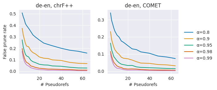
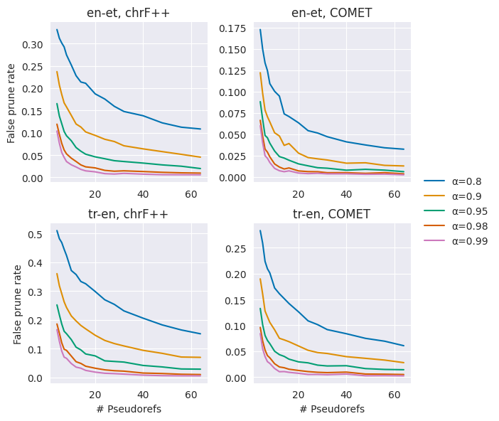
For the pseudo-reference sample size schedule , the choice of is pivotal in the speed-accuracy trade-off; is a lower bound on the number of utility calls needed, but the bootstrap estimate is more biased when the sample size is small. In a preliminary experiment on the validation set, we measure the "false pruning rate", the rate that the estimated true winner, is pruned under different choices of and . Based on results shown in Figure 1, we set to 8 for COMET and 16 for chrF++ for all experiments. are set by doubling at each time step until reaching 256.
More experimental details and figures for language pairs not shown here are in the Appendix. Our code is publicly available222https://github.com/juliusc/pruning_mbr.
4.1 Speed-accuracy trade-off
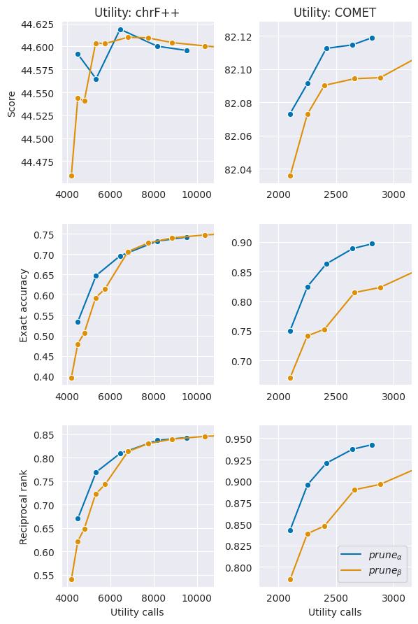
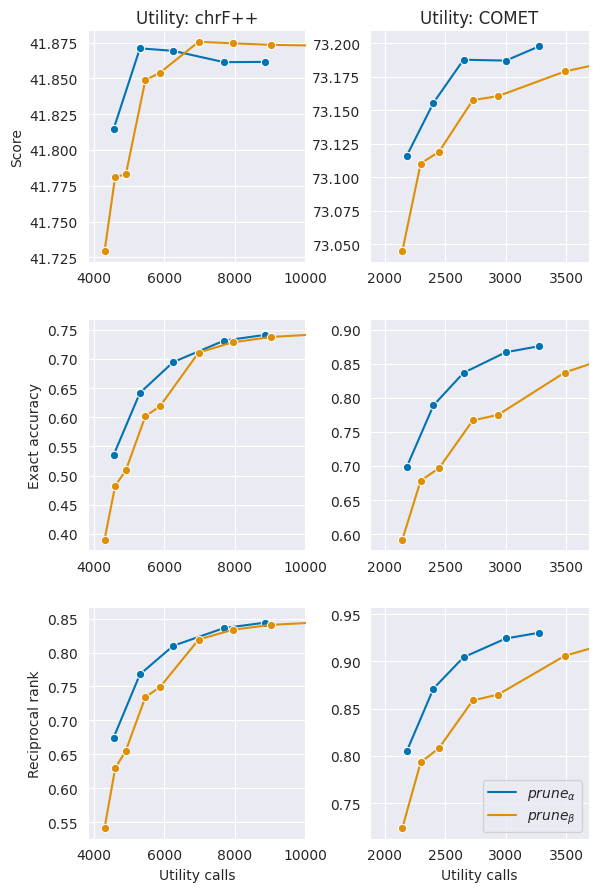
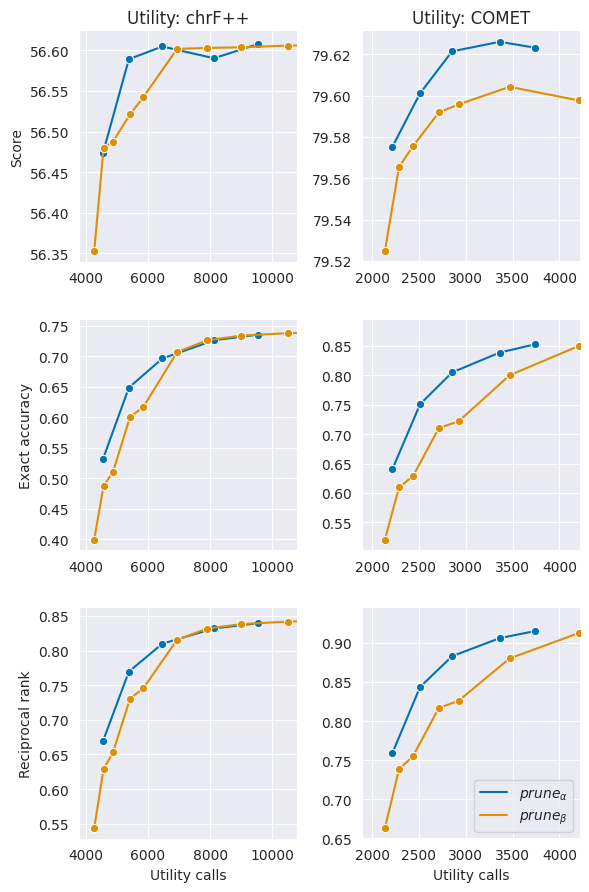
and allow control over the speed-accuracy trade-off with a single parameter. We observe this trade-off over the validation set by comparing the number of utility function calls made against various measures of accuracy. High evaluation score is underlying goal, but we find that the score changes very little across settings, so we also evaluate pruning quality in terms of how well final predictions match those under standard MBR with . We use exact accuracy, whether the prediction equals , and reciprocal rank (RR), equal to as a soft accuracy measure adapted from the mean reciprocal rank used in search (Craswell, 2009). Figure 2 shows that generally outperforms on all metrics.
4.2 Test results
| Metric: chrF++ | |||||||||
|---|---|---|---|---|---|---|---|---|---|
| de-en | en-et | tr-en | |||||||
| Score | 62.18 | 62.19 | 62.11 | 46.47 | 46.48 | 46.44 | 42.63 | 42.63 | 42.64 |
| Accuracy | 0.749 | 0.736 | 0.648 | 0.741 | 0.728 | 0.639 | 0.761 | 0.751 | 0.660 |
| RR | 0.850 | 0.840 | 0.769 | 0.843 | 0.833 | 0.762 | 0.857 | 0.850 | 0.779 |
| # Pseudo-refs | 256.0 | 234.9 | 185.2 | 256.0 | 235.3 | 188.5 | 256.0 | 238.7 | 185.7 |
| # Utility calls | 65082 | 9542 | 5402 | 63898 | 9644 | 5386 | 65356 | 8761 | 5275 |
| Metric: COMET | |||||||||
|---|---|---|---|---|---|---|---|---|---|
| de-en | en-et | tr-en | |||||||
| Score | 78.37 | 78.37 | 78.41 | 82.75 | 82.74 | 82.74 | 73.70 | 73.68 | 73.65 |
| Accuracy | 0.872 | 0.844 | 0.742 | 0.924 | 0.898 | 0.830 | 0.897 | 0.878 | 0.791 |
| RR | 0.930 | 0.911 | 0.838 | 0.959 | 0.943 | 0.898 | 0.944 | 0.932 | 0.873 |
| # Pseudo-refs | 256.0 | 200.3 | 120.4 | 256.0 | 151.4 | 82.6 | 256.0 | 177.8 | 100.8 |
| # Utility calls | 65082 | 3831 | 2533 | 63898 | 2813 | 2250 | 65356 | 3244 | 2394 |
We evaluate our methods on the test set with and and compare them to standard MBR on the accuracy metrics described in Section 4.1 as well as the number of utility calls and pseudo-references used. Table 1 shows that across all language pairs and metrics, our method achieves similar evaluation scores as standard MBR while using much less computation, with the most dramatic case being en-et and COMET with which uses 3.5% as many utility calls and 32% as many pseudo-references as the baseline.
When comparing with , we see that while exact accuracy and RR differ, the evaluation score differs very little if at all, suggesting that high-ranking hypotheses are often equally good as one another, and finely discriminating between them has diminishing returns.
4.3 Human evaluation
We confirm that our method is indistinguishable from standard MBR in human evaluation. On the de-en test set, for each instance, we sample 256 pseudo-references without replacement from and use this pool to decode with both standard MBR and . 85% of the predictions are the same, and for the rest, we asked bilingual readers of German and English to state which prediction they preferred. We obtained 125 ratings. The standard MBR prediction won in 48 cases, lost in 42, and tied in 35. This fails the significance test of Koehn (2004), so we conclude that with is not significantly different from standard MBR on de-en.
4.4 Run times
To measure realistic run times, we implement a practical version of our algorithm and compare our method against standard MBR decoding and beam search. We run our algorithm with COMET as the utility function and . With COMET, sentence embeddings can be cached, which greatly speeds up utility function calls. Some of the theoretical gains seen in Section 4.2 are diminished in practice due to our iterative algorithm dividing computations over smaller batches. Our best implementation samples all 256 pseudo-references at once but generates pseudo-reference sentence embeddings as needed. We run each algorithm on a set of 100 randomly sampled test instances. Further implementation details are given in Appendix A.2. Table 2 provides a detailed breakdown of run times. As expected, our method achieves the greatest time savings on utility computation. However, it is still substantially slower than beam search.
| Run time (seconds) | |||
|---|---|---|---|
| Prune MBR | Std. MBR | Beam | |
| Generate | 36.56 | 36.56 | 26.79 |
| Generate | 59.92 | 59.92 | |
| Embed sentences | 100.50 | 108.33 | |
| Compute utilities | 12.96 | 193.01 | |
| Bootstrap pruning | 0.63 | ||
| Total | 210.57 | 397.82 | 26.79 |
5 Conclusion
We propose an iterative pruning algorithm for MBR along with a pruning criterion based on confidence estimates derived from bootstrap resampling. In experiments across diverse language pairs and metrics, we show that our method consistently outperforms our proposed baseline and achieves significant computational savings over standard sampling-based MBR without sacrificing accuracy. Our method is a drop-in substitute for standard MBR that requires no knowledge about the model , how is generated, or the utility function.
Limitations
Even with our pruning algorithm, MBR is many times more costly to run than beam search.
An important hyperparameter in our method is the sample size schedule. We show why it is important to carefully choose the size of the first sample, but not how the remaining schedule should be set, opting to simply double the size at each step. We leave this issue to future work.
Methods such as MBR and reranking that directly optimize a metric may exploit noise in the metric to improve the score without actually improving quality (Fernandes et al., 2022). In these settings, automatic evaluation is less trustworthy and should ideally be combined with human evaluation. However, human evaluation is difficult and expensive to obtain.
Acknowledgements
Julius Cheng is supported by a scholarship from Huawei. The authors would like to thank the bilingual readers who helped with the human evaluation and the anonymous reviewers for their helpful suggestions.
References
- Bertsch et al. (2023) Amanda Bertsch, Alex Xie, Graham Neubig, and Matthew R. Gormley. 2023. It’s mbr all the way down: Modern generation techniques through the lens of minimum bayes risk.
- Bickel and Doksum (1977) P. J. Bickel and K. A. Doksum. 1977. Mathematical Statistics: Basic Ideas and Selected Topics. Holden-Day Company, Oakland, California.
- Craswell (2009) Nick Craswell. 2009. Mean Reciprocal Rank, pages 1703–1703. Springer US, Boston, MA.
- Efron (1979) B. Efron. 1979. Bootstrap Methods: Another Look at the Jackknife. The Annals of Statistics, 7(1):1 – 26.
- Eikema and Aziz (2020) Bryan Eikema and Wilker Aziz. 2020. Is MAP decoding all you need? the inadequacy of the mode in neural machine translation. In Proceedings of the 28th International Conference on Computational Linguistics, pages 4506–4520, Barcelona, Spain (Online). International Committee on Computational Linguistics.
- Eikema and Aziz (2022) Bryan Eikema and Wilker Aziz. 2022. Sampling-based approximations to minimum Bayes risk decoding for neural machine translation. In Proceedings of the 2022 Conference on Empirical Methods in Natural Language Processing, pages 10978–10993, Abu Dhabi, United Arab Emirates. Association for Computational Linguistics.
- Fernandes et al. (2022) Patrick Fernandes, António Farinhas, Ricardo Rei, José De Souza, Perez Ogayo, Graham Neubig, and Andre Martins. 2022. Quality-aware decoding for neural machine translation. In Proceedings of the 2022 Conference of the North American Chapter of the Association for Computational Linguistics: Human Language Technologies, pages 1396–1412, Seattle, United States. Association for Computational Linguistics.
- Freitag et al. (2023) Markus Freitag, Behrooz Ghorbani, and Patrick Fernandes. 2023. Epsilon sampling rocks: Investigating sampling strategies for minimum bayes risk decoding for machine translation.
- Freitag et al. (2022a) Markus Freitag, David Grangier, Qijun Tan, and Bowen Liang. 2022a. High quality rather than high model probability: Minimum Bayes risk decoding with neural metrics. Transactions of the Association for Computational Linguistics, 10:811–825.
- Freitag et al. (2022b) Markus Freitag, Ricardo Rei, Nitika Mathur, Chi-kiu Lo, Craig Stewart, Eleftherios Avramidis, Tom Kocmi, George Foster, Alon Lavie, and André F. T. Martins. 2022b. Results of WMT22 metrics shared task: Stop using BLEU – neural metrics are better and more robust. In Proceedings of the Seventh Conference on Machine Translation (WMT), pages 46–68, Abu Dhabi, United Arab Emirates (Hybrid). Association for Computational Linguistics.
- Freitag et al. (2021) Markus Freitag, Ricardo Rei, Nitika Mathur, Chi-kiu Lo, Craig Stewart, George Foster, Alon Lavie, and Ondřej Bojar. 2021. Results of the WMT21 metrics shared task: Evaluating metrics with expert-based human evaluations on TED and news domain. In Proceedings of the Sixth Conference on Machine Translation, pages 733–774, Online. Association for Computational Linguistics.
- Goel and Byrne (2000) Vaibhava Goel and William J Byrne. 2000. Minimum bayes-risk automatic speech recognition. Computer Speech & Language, 14(2):115–135.
- Hewitt et al. (2022) John Hewitt, Christopher Manning, and Percy Liang. 2022. Truncation sampling as language model desmoothing. In Findings of the Association for Computational Linguistics: EMNLP 2022, pages 3414–3427, Abu Dhabi, United Arab Emirates. Association for Computational Linguistics.
- Koehn (2004) Philipp Koehn. 2004. Statistical significance tests for machine translation evaluation. In Proceedings of the 2004 Conference on Empirical Methods in Natural Language Processing, pages 388–395, Barcelona, Spain. Association for Computational Linguistics.
- Ott et al. (2019) Myle Ott, Sergey Edunov, Alexei Baevski, Angela Fan, Sam Gross, Nathan Ng, David Grangier, and Michael Auli. 2019. fairseq: A fast, extensible toolkit for sequence modeling. In Proceedings of the 2019 Conference of the North American Chapter of the Association for Computational Linguistics (Demonstrations), pages 48–53, Minneapolis, Minnesota. Association for Computational Linguistics.
- Popović (2015) Maja Popović. 2015. chrF: character n-gram F-score for automatic MT evaluation. In Proceedings of the Tenth Workshop on Statistical Machine Translation, pages 392–395, Lisbon, Portugal. Association for Computational Linguistics.
- Post (2018) Matt Post. 2018. A call for clarity in reporting BLEU scores. In Proceedings of the Third Conference on Machine Translation: Research Papers, pages 186–191, Brussels, Belgium. Association for Computational Linguistics.
- Rei et al. (2022) Ricardo Rei, José G. C. de Souza, Duarte Alves, Chrysoula Zerva, Ana C Farinha, Taisiya Glushkova, Alon Lavie, Luisa Coheur, and André F. T. Martins. 2022. COMET-22: Unbabel-IST 2022 submission for the metrics shared task. In Proceedings of the Seventh Conference on Machine Translation (WMT), pages 578–585, Abu Dhabi, United Arab Emirates (Hybrid). Association for Computational Linguistics.
- Rei et al. (2020) Ricardo Rei, Craig Stewart, Ana C Farinha, and Alon Lavie. 2020. COMET: A neural framework for MT evaluation. In Proceedings of the 2020 Conference on Empirical Methods in Natural Language Processing (EMNLP), pages 2685–2702, Online. Association for Computational Linguistics.
- Shi et al. (2022) Freda Shi, Daniel Fried, Marjan Ghazvininejad, Luke Zettlemoyer, and Sida I. Wang. 2022. Natural language to code translation with execution. In Proceedings of the 2022 Conference on Empirical Methods in Natural Language Processing, pages 3533–3546, Abu Dhabi, United Arab Emirates. Association for Computational Linguistics.
- Suzgun et al. (2023) Mirac Suzgun, Luke Melas-Kyriazi, and Dan Jurafsky. 2023. Follow the wisdom of the crowd: Effective text generation via minimum Bayes risk decoding. In Findings of the Association for Computational Linguistics: ACL 2023, pages 4265–4293, Toronto, Canada. Association for Computational Linguistics.
- Vaswani et al. (2017) Ashish Vaswani, Noam Shazeer, Niki Parmar, Jakob Uszkoreit, Llion Jones, Aidan N Gomez, Ł ukasz Kaiser, and Illia Polosukhin. 2017. Attention is all you need. In Advances in Neural Information Processing Systems, volume 30. Curran Associates, Inc.
- Yan et al. (2022) Jianhao Yan, Jin Xu, Fandong Meng, Jie Zhou, and Yue Zhang. 2022. Dc-mbr: Distributional cooling for minimum bayesian risk decoding. arXiv preprint arXiv:2212.04205.
Appendix A Additional experimental details
A.1 All experiments
Preliminary experiments showed no significant difference between 500 and 1000 bootstrap samples when running , so we use 500 for all experiments.
For efficiency, we use average sentence-level chrF++ instead of corpus-level chrF++ for corpus-level evaluations. This allows us to pre-compute the sentence-level chrF++ for each hypothesis and obtain the corpus-level score of a set of predictions by simple averaging.
All experiments are implemented on top of our fork of Fairseq (Ott et al., 2019).
A.2 Run times
This section contains additional details for the experiment in Section 4.4.
For both the standard and pruning MBR algorithms, we deduplicate and cache computations whenever possible. For each unique pseudo-reference, its sentence embedding and utility scores against each are only computed once.
For simplicity, all decoding methods are run on one sequence at a time. Batching across sequences would likely affect the relative performance characteristics of each method.
All experiments are conducted on the same machine with one Nvidia Quadro RTX 8000 GPU.
Appendix B False pruning rates for en-et, tr-en
Figure 3 shows the false pruning rates for en-et and tr-en.
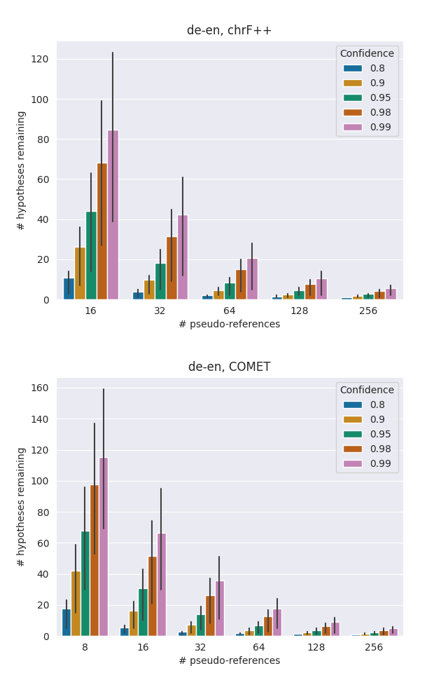
Appendix C Hypotheses remaining per time step
Figure 4 shows the distribution of the number of remaining hypotheses after each time step when running our method on the de-en validation set, following the experimental setup of Section 4.1 where . This is provided to further illustrate the pruning process.
Appendix D Speed-accuracy trade-off for en-et, tr-en