Faster Algorithms for Cycle Hitting Problems on Disk Graphs^††thanks: This work was supported by the National Research Foundation of Korea(NRF) grant funded by the Korea government(MSIT) (No.RS-2023-00209069)

We first apply a branching process as follows to obtain $2^{O((k/p)\log k)}$ instances one of which is a YES-instance $(G^{\prime},k^{\prime})$ of Triangle Hitting Set where every clique of $G^{\prime}$ has size $O(p)$. For a clique $C$ of $G$ and a triangle hitting set $F$, all except for at most two vertices of $C$ are contained in $F$. In particular, if $G$ has a triangle hitting set of size $k$, any clique of $G$ has size at most $k+2$. For a clique of size at least $p$, we branch on which vertices of the clique are not included in a triangle hitting set. After this, the solution size $k$ decrease by at least $p-2$. We repeat this until every clique has size $O(p)$. In the resulting branching tree, every node has at most $O(k^{2})$ children since any clique of $G$ has size at most $k+2$. And the branching tree has height $O(k/p)$. In this way, we can obtain $2^{O((k/p)\log k)}$ instances of Triangle Hitting Set one of which is a YES-instance $(G^{\prime},k^{\prime})$ of Triangle Hitting Set where $G^{\prime}$ has a geometric representation of ply at most $p$. Moreover, $G^{\prime}$ is an induced subgraph of $G$, and $k^{\prime}\leq k$. Using the EPTAS for computing a maximum clique in a disk graph [8], we can complete the branching step in $2^{O((k/p)\log k)}n^{O(1)}$ time. Note that the algorithm in [8] does not require a geometric representation of a graph.

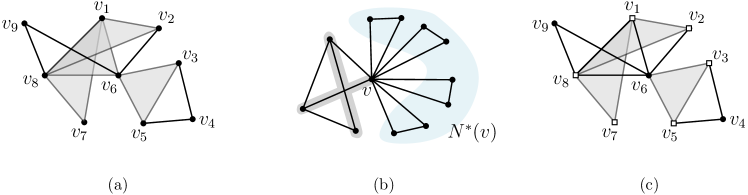
For each instance $(G,k)$ obtained from the first branching, we apply the second branching process to obtain $2^{O(k/p)}$ instances one of which is a YES-instance having a core of size $O(pk)$. A set $W$ of triangles of $G$ is called a core if for a triangle of $G$, a triangle of $W$ shares at least two vertices with the triangle. See Fig. 1(a). During the branching process, we mark an edge to remember that one of its endpoints must be added to a triangle hitting set. The marking process has an invariant that no two marked edges share a common endpoint, and thus the number of marked edges is at most $k$. The marks will be considered in the dynamic programming procedure. Initially, all edges are unmarked.

Let $v$ be a vertex such that $N^{*}(v)$ has a matching of size at least $p$, where $N^{*}(v)$ be the set of neighbors of $v$ not incident to any marked edge. See Fig. 1(b). In this case, a triangle hitting set contains either $v$ or at least one endpoint of each edge in the matching. We branch on whether or not $v$ is added to a triangle hitting set. For the first case, we remove $v$ and its adjacent edges, and decrease $k$ by one. For the second case, we know that at least one endpoint of each edge in the matching must be contained in a triangle hitting set. However, we do not make a decision at this point. Instead, we simply mark all such edges.

This branching process was already used in [17]. The following lemma is a key for our improvement over [17].

At this moment, $W$ is not necessarily a core. See Fig. 1(c). Thus we add several triangles further to $W$ to compute a core of $G$. By the branching process, for every vertex $v$ of $F_{0}$, $N(v)\setminus F_{0}$ has a maximum matching of size at most $p$. We add the triangles formed by $v$ and the edges of the maximum matching to $W$ for every vertex $v$ of $F_{0}$. Note that we do not update $F_{0}$ during this phase, and thus triangles added to $W$ due to two different vertices might intersect. This algorithm clearly runs in polynomial time. Moreover, since the size of $F_{0}$ is $O(k)$, we add at most $O(pk)$ triangles to $W$, and thus the size of $W$ is $O(pk)$.

We claim that $W$ is a core of $G$. Let $\{x,y,z\}$ be a triangle of $G$ not in $W$. Since $F_{0}$ contains a triangle hitting set of size at most $3k$, it must contain at least one of $x,y$ and $z$. If at least two of them, say $x$ and $y$, are contained in $F_{0}$, then there exists a triangle having edge $xy$ in $W$ by construction. Thus, $\{x,y,z\}$ shares two vertices with such a triangle. The remaining case is that exactly one of them, say $x$, is contained in $F_{0}$. In this case, we have considered $x$ and a maximum matching of $N(x)\setminus F_{0}$. The only reason why $\{x,y,z\}$ is not added to $W$ is that the edge $yz$ is adjacent to another edge $y^{\prime}z^{\prime}$ for some other triangle $\{x,y^{\prime},z^{\prime}\}$. Then $\{x,y^{\prime},z^{\prime}\}$ is added to $W$. Note that $\{x,y,z\}$ and $\{x,y^{\prime},z^{\prime}\}$ share at least two vertices, and thus $\{x,y,z\}$ satisfies the condition for $W$ being a core.    

The following observation will be used in the correctness proof of the kernelization step in Section 3.2. The observation holds because $G^{\prime}$ does not have any triangle not appearing in $G$. {observation} Let $G^{\prime}$ be an induced subgraph of $G$ such that $V(G^{\prime})$ contains all vertices of a core $W$ of $G$. Then $W$ is a core of $G^{\prime}$.

For each instance $(G,k)$ obtained from the branching process, we apply the cleaning step that removes all vertices not hitting any triangle of $G$ from $G$. Specifically, we remove a vertex of degree less than two. Also, we remove a vertex whose neighbors are independent. Whenever we remove a vertex, we also remove its adjacent edges.

Let $(G,k)$ be a YES-instance we obtained from the branching process. We show that if the number of vertices of $G$ contained in the triangles of $G$ is at least $pk$, we can construct a crown for the triangles of $G$. Then using this, we can produce a YES-instance $(G^{\prime},k)$ of Triangle Hitting Set in polynomial time where $G^{\prime}$ is a proper induced subgraph of $G$. Thus by repeatedly applying this process (at most $n^{2}$ times) and then by removing all vertices not contained in any triangle of $G$, we can obtain a YES-instance $(G^{\prime},k)$ where $G^{\prime}$ is a disk graph of complexity $O(pk)$.

We first define a crown decomposition of a graph for triangles. For illustration, see Fig. 2. A crown decomposition of a graph was initially introduced to construct a linear kernel for Vertex Cover. Later, Abu-Khzam [1] generalized this concept to hypergraphs. Using this, he showed that a triangle hitting set admits a quadratic kernel for a general graph. In our case, we will show that the size of a kernel is indeed $O(pk)$ due to the branching process. More specifically, it is due to the existence of a core of size $O(pk)$.

If a crown $(I,H,M)$ for the triangles of $G$ exists, we can remove all vertices in $I$, but instead, we mark all edges of $H$. Then the resulting graph also has a triangle hitting set of size at most $k$ [1].

We claim that $F^{\prime}$ is also a triangle hitting set. A triangle not intersecting $I$ is hit by $F^{\prime}$ by construction. Thus consider a triangle $\{x,u,v\}$ intersecting $I$. Since no two vertices of $I$ are contained in the same triangle, exactly one of $x,u$ and $v$, say $x$, is contained in $I$. Since every edge of $H$ is matched under $M$, $uv\in H$. Since $F^{\prime}$ contains either $u$ or $v$, $\{x,u,v\}$ is hit by $F^{\prime}$. Therefore, $F^{\prime}$ is a triangle hitting set of size at most $k$.    

Now we show that $(G,k)$ has a crown for its triangles if $cpk$ vertices are contained in the triangles of $G$, where $c$ is a sufficiently large constant. Let $W$ be a core of $G$ of size $O(pk)$, which exists due to Lemma 6 and Observation 3.1. Let $I$ be the set of vertices of $G$ not contained in any triangle of $W$ but contained in some triangle of $G$. If $cpk$ vertices are contained in the triangles of $G$, the size of $I$ is $c^{\prime}pk$ for a sufficiently large constant $c^{\prime}$ since $|W|=O(pk)$. Then let $H$ be the set of all edges of $G$ which form triangles together with the vertices of $I$. Note that for every edge of $H$, its endpoints are contained in the same triangle of $W$ by the definition of the core. Thus the size of $H$ is at most $3\cdot|W|=O(pk)$. Therefore, if more than $cpk$ vertices are contained in the triangles of $G$, $|I|>|H|$.

Then we show that $(I^{\prime},H^{\prime},M^{\prime})$ is a crown for the triangles of $G$. First, $I^{\prime}$ does not violate the condition in Definition 1 since $I^{\prime}\subset I$. Then consider the condition for $H^{\prime}$. Note that $H^{\prime}$ is contained in $X$, and $I^{\prime}$ does not intersect $X$. Thus for all triangles $\{x,u,v\}$ with $x\in I^{\prime}$, $uv$ must be in $H$, and then $uv$ must be in $H^{\prime}$. Therefore, $H^{\prime}$ is the set of all edges of $G^{\prime}$ that form triangles together with the vertices of $I^{\prime}$, and thus $H^{\prime}$ satisfies the secons condition in Definition 1. Also, by construction, $G_{I^{\prime},H^{\prime}}$ is a subgraph of $G_{I,H}$ such that all edges of $M^{\prime}$ are in $G_{I^{\prime},H^{\prime}}$, and thus $H^{\prime}$ are matched under $M^{\prime}$.    

By Lemma 8 and Lemma 9, we can obtain an instance $(G^{\prime},k^{\prime})$ equivalent to $(G,k)$ such that the union of the triangles has complexity $O(pk)$ for each instance $(G,k)$ obtained from Section 3.1 in polynomial time.

By applying dynamic programming on $(T,\beta)$ as described in Lemma 16, we can find a triangle hitting set of size $k^{\prime}$ in $2^{O(\sqrt{pk})}$ time if it exists. Therefore, the total running time is $2^{O(\sqrt{pk})}\cdot 2^{O((k/p)\log k)}$. By letting $p=k^{1/3}$, we have $2^{O(k^{2/3}\log k)}n^{O(1)}$-time.

If we are not given a geometric representation, we cannot use a tree decomposition of bounded weighted width. Instead, we can compute a tree decomposition $(T,\beta)$ of $G^{\prime}$ of treewidth $O(p\sqrt{pk})$. Then the total running time is $2^{O(p^{3/2}\sqrt{k})}\cdot 2^{O((k/p)\log k)}$. By letting $p=k^{1/5}$, we have $2^{O(k^{4/5}\log k)}n^{O(1)}$-time.    

Let $(G,k)$ be an YES-instance obtained from the branching and cleaning process. Let $F$ be a subset of $V(G)$ containing a core of $G$. The disks of $G-F$ have ply at most two. In this section, we give an upper bound on the number of deep vertices for $F$. For this, we classify the vertices of $V-F$ in two types: regular and irregular vertices. See Fig. 3(a).

Since each clique has size at most $p$, a deep and regular vertex has at most $2p$ neighbors in $G$. Let $v$ be a deep and regular vertex having exactly $r$ neighbors. Consider the additively weighted order-$r$ Voronoi diagram $r\textsf{VD}$ of $F$. Here, the distance between a disk $D^{\prime}$ of $F$ and a point $x$ in the plane is defined as $d(c,x)-w$, where $c$ is the center of $D^{\prime}$ and $w$ is the radius of $D^{\prime}$. Then the center of $D(v)$ is contained in a Voronoi region of the order-$r$ Voronoi diagram whose sites are exactly the neighbors of $v$. Since no two deep vertices have the same neighborhood in $F$, each Voronoi region contains at most one deep vertex. Therefore, the number of deep and regular vertices having exactly $r$ neighbors is linear in the complexity of $r\textsf{VD}$ for $r\leq 2p$. By Lemma 4, its complexity is $O(r|F|)$. Thus, the number of deep and regular vertices of $G$ is $O(p^{2}|F|)$.    

For irregular vertices, we make use of the fact that the ply of the disks represented by those vertices is at most two. It is not difficult to see that the number of irregular vertices of the first three types is $O(p|F|)$. This is because the complexity of $\mathcal{A}$ is $O(p|F|)$. To analyze the number of irregular vertices of the fourth type, we use the following lemma.

By the Euler’s formula, $|E_{H}|\leq|V_{H}|+|F_{1}|+|F_{2}|-2$, where $V_{H}$ and $E_{H}$ denote the set of vertices and edges of $H$, respectively. Note that no vertex of $H$ has degree at most one. Since every face of $F_{2}$ is incident to at least three edges of $H$, and every edge of $E_{H}$ is incident to exactly two faces of $H$, $2|E_{H}|\geq 3|F_{2}|+2|F_{1}|$. Thus we have $2|F_{1}|+3|F_{2}|\leq 2|V_{H}|+2|F_{1}|+2|F_{2}|-4$. That is, $|F_{2}|\leq 2|V_{H}|-4$. This implies the first part of the lemma.

Now consider the second part of the lemma. Since a pair of vertices has at most two parallel edges, $|F_{1}|\leq|E_{H}|/2$. Therefore, $|E_{H}|\leq 2|V_{H}|+2|F_{2}|-4=O(|V_{H}|)$. Since every edge of the regions of $\mathcal{F}$ corresponds to an edge of $H$, the total number of edges of the regions of $\mathcal{F}$ is $O(|S|)$, and thus the total number of vertices of them is $O(|S|)$.    

In this section, we show how to compute a feedback vertex set of size $k$ in $2^{\tilde{O}(k^{7/8})}n^{O(1)}$ time, if it exists. Without a geometric representation of $G$, we can do this in $2^{\tilde{O}(k^{9/10})}n^{O(1)}$ time. Let $(G,k)$ be an YES-instance of Feedback Vertex Set from the branching and cleaning processes. Then we have a core $W$ of $G$ of size $O(pk)$. Let $F$ be the union of a feedback vertex set of size $2k$ and the vertex set of all triangles of core $W$ of $G$, and let $F^{*}$ be the union of $F$ and all deep vertices for $F$. The size of $F^{*}$ is $O(p^{3}k)$ by Lemmas 11 and 13. Since $F^{*}$ contains a feedback vertex set, $G-F^{*}$ is a forest.

References

- [1] Abu-Khzam, F.N.: A kernelization algorithm for -hitting set. Journal of Computer and System Sciences 76(7), 524–531 (2010)
- [2] An, S., Oh, E.: Feedback Vertex Set on Geometric Intersection Graphs. In: Proceedings of the 32nd International Symposium on Algorithms and Computation (ISAAC 2021). pp. 47:1–47:12 (2021)
- [3] Bandyapadhyay, S., Lochet, W., Lokshtanov, D., Saurabh, S., Xue, J.: Subexponential parameterized algorithms for cut and cycle hitting problems on H-minor-free graphs. In: Proceedings of the 2022 Annual ACM-SIAM Symposium on Discrete Algorithms (SODA). pp. 2063–2084. SIAM (2022)
- [4] Bandyapadhyay, S., Lochet, W., Lokshtanov, D., Saurabh, S., Xue, J.: True contraction decomposition and almost eth-tight bipartization for unit-disk graphs. In: 38th International Symposium on Computational Geometry (SoCG 2022). vol. 224, pp. 11:1–11:16 (2022)
- [5] de Berg, M., Bodlaender, H.L., Kisfaludi-Bak, S., Marx, D., Zanden, T.C.v.d.: A framework for Exponential-Time-Hypothesis–tight algorithms and lower bounds in geometric intersection graphs. SIAM Journal on Computing 49(6), 1291–1331 (2020)
- [6] de Berg, M., Kisfaludi-Bak, S., Monemizadeh, M., Theocharous, L.: Clique-based separators for geometric intersection graphs. In: 32nd International Symposium on Algorithms and Computation (ISAAC 2021). pp. 22:1–22:15 (2021)
- [7] Bodlaender, H.L., Cygan, M., Kratsch, S., Nederlof, J.: Deterministic single exponential time algorithms for connectivity problems parameterized by treewidth. Inf. Comput. 243, 86–111 (2015)
- [8] Bonamy, M., Bonnet, E., Bousquet, N., Charbit, P., Giannopoulos, P., Kim, E.J., Rzążewski, P., Sikora, F., Thomassé, S.: EPTAS and subexponential algorithm for maximum clique on disk and unit ball graphs. Journal of the ACM 68(2) (2021)
- [9] Breu, H., Kirkpatrick, D.G.: Unit disk graph recognition is NP-hard. Computational Geometry 9(1-2), 3–24 (1998)
- [10] Cygan, M., Fomin, F.V., Kowalik, L., Lokshtanov, D., Marx, D., Pilipczuk, M., Pilipczuk, M., Saurabh, S.: Parameterized Algorithms. Springer Publishing Company, Incorporated (2015)
- [11] Demaine, E.D., Fomin, F.V., Hajiaghayi, M., Thilikos, D.M.: Subexponential parameterized algorithms on bounded-genus graphs and H-minor-free graphs. Journal of the ACM (JACM) 52(6), 866–893 (2005)
- [12] Fomin, F.V., Lokshtanov, D., Panolan, F., Saurabh, S., Zehavi, M.: Decomposition of map graphs with applications. In: Proceedings of the 46th International Colloquium on Automata, Languages, and Programming (ICALP 2019). pp. 60:1–60:15 (2019)
- [13] Fomin, F.V., Lokshtanov, D., Panolan, F., Saurabh, S., Zehavi, M.: Finding, hitting and packing cycles in subexponential time on unit disk graphs. Discrete & Computational Geometry 62(4), 879–911 (2019)
- [14] Fomin, F.V., Lokshtanov, D., Saurabh, S.: Bidimensionality and geometric graphs. In: Proceedings of the Twenty-Third Annual ACM-SIAM Symposium on Discrete Algorithms (SODA 2012). pp. 1563–1575 (2012)
- [15] Li, J., Nederlof, J.: Detecting feedback vertex sets of size in time. In: Proceedings of the Fourteenth Annual ACM-SIAM Symposium on Discrete Algorithms (SODA 2022). pp. 971–989 (2020)
- [16] Lokshtanov, D., Narayanaswamy, N., Raman, V., Ramanujan, M., Saurabh, S.: Faster parameterized algorithms using linear programming. ACM Transactions on Algorithms (TALG) 11(2), 1–31 (2014)
- [17] Lokshtanov, D., Panolan, F., Saurabh, S., Xue, J., Zehavi, M.: Subexponential parameterized algorithms on disk graphs (extended abstract). In: Proceedings of the 2022 Annual ACM-SIAM Symposium on Discrete Algorithms (SODA 2022). pp. 2005–2031
- [18] Lokshtanov, D., Saurabh, S., Wahlström, M.: Subexponential parameterized odd cycle transversal on planar graphs. In: IARCS Annual Conference on Foundations of Software Technology and Theoretical Computer Science (FSTTCS 2012). Schloss Dagstuhl-Leibniz-Zentrum fuer Informatik (2012)
- [19] Rosenberger, H.: Order- voronoi diagrams of sites with additive weights in the plane. Algorithmica 6(1), 490–521 (1991)
- [20] Wahlström, M.: Algorithms, measures and upper bounds for satisfiability and related problems. Ph.D. thesis, Department of Computer and Information Science, Linköpings universitet (2007)