Fast Radio Bursts with Narrow Beaming Angles Can Escape from Magnetar Magnetospheres

It has been seventeen years since the first fast radio burst (FRB) was discovered (Lorimer et al., 2007). Despite significant achievements in this field, many problems remain unresolved, including the origin and radiation mechanism of FRBs. The magnetar origin of at least some FRBs has been confirmed by the association of FRB 200428 with the galactic magnetar SGR 1935+2154 (Bochenek et al., 2020; CHIME/FRB Collaboration et al., 2020). Nevertheless, the inferred isotropic peak luminosities of the bursts detected from SGR 1935+2154 are apparently smaller than those of bursts at cosmological distances (Zhang et al., 2020; Kirsten et al., 2021; Dong & Chime/Frb Collaboration, 2022; Pearlman & Chime/Frb Collaboration, 2022). The radiation mechanism of FRBs is also puzzling. Releasing a large amount of energy within one millisecond implies that their radiation is highly coherent, which may be somewhat challenging to understand.

Various radiation models have been proposed based on the hypothesis that FRBs originate from neutron stars. In general, these models can be broadly classified into two main categories: magnetospheric models (Kumar et al., 2017; Yang & Zhang, 2018; Lu et al., 2020; Wang et al., 2022b; Zhang, 2022; Liu et al., 2023; Qu & Zhang, 2024) and far-away models (Lyubarsky, 2014; Beloborodov, 2017, 2020; Metzger et al., 2019; Margalit et al., 2020). Accumulated observations indicate that FRBs share some similarities with pulsars, which therefore favors their magnetospheric origin. Some potential observational evidence includes: frequency drifting (CHIME/FRB Collaboration et al., 2019; Hessels et al., 2019; Pleunis et al., 2021; Zhou et al., 2022), evolution of polarization position angles (Cho et al., 2020; Luo et al., 2020; Mckinven et al., 2024; Niu et al., 2024), sub-second periodicity (Chime/Frb Collaboration et al., 2022), nanosecond temporal variability (Majid et al., 2021; Nimmo et al., 2022), and scintillation (Nimmo et al., 2024), etc. Recently, some discussions on the polarization property (Wang et al., 2022a; Qu & Zhang, 2023; Jiang et al., 2024; Liu et al., 2024; Zhao & Wang, 2024), narrow spectrum (Yang, 2023; Kumar et al., 2024; Wang et al., 2024), and waiting-time distribution (Xiao et al., 2024) of FRBs also provide clues to the magnetospheric origin.

However, a potential issue for magnetospheric origin is that FRBs could be scattered by a magnetospheric dense plasma, which makes it difficult for them to escape (Beloborodov, 2021, 2022, 2023). This can be attributed to two reasons. The first reason is the enhancement of the scattering cross section due to the strong wave effect of FRBs. The second reason, perhaps more importantly, is that the plasma accelerated by an FRB pulse can emit high-energy gamma photons through curvature radiation. These photons collide with each other and generate considerable electron–positron plasma through the reaction $\gamma+\gamma\to e^{-}+e^{+}$, thereby boosting the plasma number density. Although subsequent studies pointed out that the scattering cross section of particles can be reduced if the angle between the FRB propagation direction and the local magnetic field is small or the pre-wave plasma has an extremely relativistic outflow (Qu et al., 2022; Lyutikov, 2024), the issue of additional electron–positron-pair creation has not been thoroughly solved yet so far. Therefore, whether FRBs can escape from magnetar magnetospheres still remains a topic which is worthy of research.

This paper is organized as follows. In Section 2, we briefly summarize the scattering issue of FRBs in magnetar magnetospheres. In Section 3, we reinvestigate the motion of a magnetospheric particle under the influence of an FRB by generalizing the result of Beloborodov (2021, 2022) to the case of oblique propagation. The Lorentz factor of the particle is boosted by the FRB, leading to an enhancement in the scattering cross section. On the one hand, the particle has a nearly constant velocity component along the direction of the background magnetic field, depending on the angle between the FRB propagation direction and the field line. On the other hand, the particle exhibits significant gyration around the field line. Such gyration is responsible for producing a large number of high-energy photons that contribute to the reaction $\gamma+\gamma\to e^{-}+e^{+}$. In Section 4, we discuss several approaches to reduce the scattering effect. We find that: (1) When the angle between the FRB propagation direction and the background magnetic field line is $\theta\lesssim 10^{-2}\text{ rad}$, pair creation can be effectively inhibited. (2) For an FRB with a small transverse spatial size, the pair creation can also be significantly reduced. This effect becomes significant primarily when the propagation angle $\theta\sim 10^{-1}\text{ rad}$. Based on this result, we then constrain the beaming angle and emission radius of FRBs in stellar magnetospheres. The main discussion is presented in Section 5. We adopt the notation $Q_{n}=Q/10^{n}$ and cgs units in the whole paper.

The calculations in the previous section assume that the propagation direction of the FRB is perpendicular to the background magnetic field line. In fact, an FRB is more likely to propagate obliquely relative to the field line. In this section, we will generalize above results to the case of oblique propagation.

We first establish a coordinate system in the lab frame, as shown in the left panel of Figure 3. We assume an FRB is propagating along the $z-$ axis. The electric field and magnetic field of the FRB are along the $x-$ and $y-$ axes, respectively. The background magnetic field is assumed to be in the $y-z$ plane, and has an angle $\theta$ with respect to the $z-$ axis. One can also define a reference frame $K^{\prime}$ that is sliding along the background magnetic field line with a Lorentz factor $\gamma_{f}=1/\sin{\theta}$. An advantage in such a reference frame is that the magnetic field direction of the FRB is aligned with the background magnetic field. A corresponding coordinate system thus can be established in this frame, as shown in the right panel of Figure 3 (we use a prime symbol to denote the quantity in the frame $K^{\prime}$). The relativistic transformations between the frame $K^{\prime}$ and the lab frame are (Huang et al., 2024)

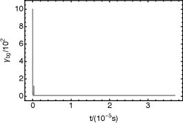
An example for the motion of a test particle in the lab frame is shown in Figure 4. The motion of the particle has three interesting properties. Firstly, the Lorentz factor $\gamma$ is boosted to a high value by continuous resonance events. Secondly, the velocity of the particle along the field line $\beta_{\text{bg}}$ quickly drops down and finally becomes nearly constant. Thirdly, the particle exhibits significant gyration around the field line. One can also simulate the motion of the particle independently in the frame $K^{\prime}$ by adopting the same parameters as those in Figure 4 from relativistic transformations (19). The motion of the particle in the frame $K^{\prime}$ is shown in Figure 5. Although the particle possesses a high Lorentz factor $\gamma^{\prime}$ and also exhibits significant gyration around the field line, its velocity component along the field line nearly vanishes. This is compatible with that observed in the lab frame, i.e., the particle nearly slides along the field line at the same velocity as the reference frame $K^{\prime}$,

This phenomenon can be explained as follows. Let us assume that the particle possesses an initial Lorentz factor $\gamma_{i}\gg 1$ along the field line in the lab frame.¹¹1In fact, $\gamma_{i}\gg 1$ is controversial (Beloborodov, 2023). However, we show here that even if the initial Lorentz factor $\gamma_{i}\gg 1$, it cannot effectively influence the motion of a particle in an FRB. The Lorentz factor $\gamma_{i}$ corresponds to an initial velocity

This velocity observed in the frame $K^{\prime}$ can be derived by a relativistic transformation,

which corresponds to a Lorentz factor

where in the second equality, we have assumed $\gamma_{i}^{2}\left(1-\cos{\theta}\right)\gg 1/2$. When $\theta\ll 1$, one has $\gamma_{i}^{\prime}\approx\gamma_{i}\theta/2$. This indicates that any large initial Lorentz factor in the lab frame will be reduced by a factor $\theta/2$ in the frame $K^{\prime}$. For example, when $\gamma_{i}=1000$ and $\theta=10^{-1}\text{ rad}$, the initial Lorentz factor $\gamma_{i}^{\prime}\approx 50$, as shown in the upper middle panel of Figure 5.

In the reference frame $K^{\prime}$, along the direction of the field line, the particle only experiences a radiation reaction force, which is anti-parallel to the direction of its velocity. Therefore, the momentum component of the particle along the field line loses continuously, as shown in the lower left panel of Figure 5. One then has

where we have used Equation (6) but in the frame $K^{\prime}$,

In conclusion, a large initial Lorentz factor ($\gamma_{i}\sim 1000$) in the lab frame is not important to influence the motion of the particle when $\theta\ll 1$. Once the particle is exposed in the FRB pulse, its velocity along the background magnetic field line quickly synchronizes with the velocity of the frame $K^{\prime}$, which is given by Equation (20).

The Lorentz factor $\gamma^{\prime}$ in the frame $K^{\prime}$ corresponds to a velocity $\beta^{\prime}\approx\left(1-1/\gamma^{\prime 2}\right)^{1/2}$, which is almost perpendicular to the field line. In the lab frame, the velocity perpendicular to the field line is obtained by a relativistic transformation, $\beta_{\text{bg},\perp}\approx\beta^{\prime}/\gamma_{f}$. Therefore, the Lorentz factor of the particle in the lab frame is

where we use the tilde symbol to denote the generalization of the quantity in the case of oblique propagation. Although the Lorentz factor is boosted by a factor $\gamma_{f}^{13/8}$ compared to the perpendicular case, the emission power of the particle is reduced. A general expression of the total emission power of a particle oscillating in an FRB is (Beloborodov, 2022; Huang et al., 2024)

where we have used $\beta_{z}\approx\beta_{\text{bg}}\cos{\theta}\approx\cos^{2}{\theta}$. The emission power reduces to Equation (12) when $\theta=\pi/2$. The scattering cross section of an electron in an FRB thus is

For the case of oblique propagation, one can see that the scattering cross section is reduced by a factor $\gamma_{f}^{-3/4}$.

The generalized characteristic frequency of the curvature radiation photon is

where $\widetilde{r}_{c}$ is the generalized curvature radius, which can be estimated as follows. In the frame $K^{\prime}$, the curvature radius is

It is worthy of noting that the transverse length remains invariant under the relativistic transformation, i.e., $r_{\text{c},\text{bg},\perp}\approx r_{c}^{\prime}$. Within a time interval $2\pi r_{\text{c},\text{bg},\perp}/\left(c\beta_{\text{bg},\perp}\right)$, the distance that the particle travels along the field line is

The curvature radius of the particle’s trajectory thus can be estimated by

A propagation angle $\theta<81^{\circ}$ is more reasonable, and will be adopted in the following discussion. For $\nu=10^{9}\text{ Hz}$, $a_{0}=2000$, $\omega_{B}/\omega=40$, and $\theta=0.1\text{ rad}$, the curvature radius $\widetilde{r}_{c}\approx 1.2\times 10^{5}\text{ cm}$, which is consistent with that shown in the lower left panel of Figure 4. One can recalculate the ratio between the characteristic energy of the emitted photon and the electron rest energy,

Outside the light cylinder $R_{\text{LC}}\approx\left(4.8\times 10^{9}\text{ cm}\right)P_{0}$, the toroidal field gradually dominates the magnetic field configuration. Therefore, the characteristic energy of emitted photons is insufficient to effectively generate electron–positron pairs. We will focus on the scattering problem inside the magnetosphere.

Based on above calculations, Equation (17) ultimately can be rewritten as

One may argue that for a small propagation angle such as $\theta\sim 0.1\text{ rad}$, $\gamma_{f}^{-6}\sim 10^{-6}$ is enough to cancel out the large number of pair creation. However, if the angle $\theta$ is small, the time $T$ that the particle stays in the wave can also deviate from one millisecond significantly. This can be seen more clearly in Figure 6. In the lab frame, the particle is nearly sliding along the background magnetic field with a constant velocity $\beta_{\text{bg}}\approx\cos{\theta}$. The velocity components parallel and perpendicular to the wave vector are $\beta_{\boldsymbol{k}}=\beta_{\text{bg}}\cos{\theta}\approx\cos^{2}{\theta}$ and $\beta_{\boldsymbol{k},\perp}=\beta_{\text{bg}}\sin{\theta}\approx\sin{\theta}\cos{\theta}$, respectively. In general, there are three available choices for $T$. The first choice is the time that a particle takes to penetrate the pulse along the wave vector,

where the duration of the pulse is set as one millisecond. In this case, replacing $T=T_{\text{pen}}$ in Equation (34) is incapable of reducing the value of $\widetilde{\mathcal{M}}$ effectively. Nevertheless, another possibility is that the theoretical maximum,

is smaller than the value of $T_{\text{pen}}$. In this case, $T$ in Equation (34) should be replaced by $T_{\text{max}}$. On the one hand, in order to control pair creation ($\widetilde{\mathcal{M}}<1$), one requires

On the other hand, the lost energy of the FRB due to scattering by particles is

where $N_{e}$ is the number of particles scattering the FRB, $r$ is the radius where scattering is most severe, and $\theta_{j}$ is the radiation cone half-opening angle of the FRB pulse. The total realistic energy of the FRB is

Therefore, the ratio of energy loss is

The value of $\Delta\mathcal{E}/\mathcal{E}$ is not supposed to exceed unity, which implies

The joint constraint on $\theta$ as a function of distance $r$ by combining both $\widetilde{\mathcal{M}}<1$ and $\Delta\mathcal{E}/\mathcal{E}<1$ is shown in the left panel of Figure 7.

Another approach to reduce scattering is as follows. As we have mentioned before, the strong scattering condition $1<\omega_{B}/\omega<a_{0}$ is valid only when $\theta=\pi/2$. Therefore, the strong scattering can occur only when $1<\omega_{B}^{\prime}/\omega^{\prime}<a_{0}^{\prime}$ is satisfied in the frame $K^{\prime}$. After the relativistic transformation (19), this becomes $\sin{\theta}<\omega_{B}/\omega<a_{0}\sin{\theta}$. A critical propagation angle can be reached when

which is identical to the empirical formula obtained by Qu et al. (2022) through numerical simulation. ²²2Another explanation that gives the same critical propagation angle is presented in Qu & Zhang (2024). Therefore, another effective way to reduce scattering is to require $a_{0}\sin{\theta}<\omega_{B}/\omega$, i.e.,

The corresponding constraint on $\theta$ as a function of distance $r$ is shown in the middle panel of Figure 7. Combining the aforementioned results, one can draw a conclusion that a propagation angle $\theta\lesssim 10^{-2}\text{ rad}$ along the propagation path to the light cylinder can reduce scattering effectively. However, such an extremely small propagation angle seems somewhat unnatural unless the FRB can tilt field lines to make them get aligned with the propagation direction (Qu et al., 2022). Nevertheless, whether such a phenomenon can occur is still in doubt (Beloborodov, 2023).

Here, we propose another simple strategy to control pair creation without requiring the angle is as small as $10^{-2}\text{ rad}$. As shown in Figure 6, the time needed for the particle to cross the FRB pulse laterally is

If $T_{\text{cro}}<T_{\text{max}}$, i.e., an FRB has a sufficiently small transverse spatial size $\mathcal{D}<\left(10^{9}\text{ cm}\right)r_{9}\sin{\theta}\cos{\theta}$, then the time $T$ in Equation (34) should be replaced by $T_{\text{cro}}$. In this case, $\widetilde{M}<1$ is equivalent to

An FRB pulse with a transverse size smaller than the critical value $\mathcal{D}_{\text{cr}}$ can effectively reduce the production of electron–positron pairs. The ratio of energy loss is

Therefore, $\Delta\mathcal{E}/\mathcal{E}<1$ is equivalent to

The premise of these calculations, $T_{\text{cro}}<T_{\text{max}}$ indicates

which is opposite to Equation (37) when $\mathcal{D}=\mathcal{D}_{\text{cr}}$. The constraint on $\theta$ combing Equations (47) and (48) is shown in the right panel of Figure 7. In summary, the valid regions of these three constraints almost cover the parameter space where scattering is most severe ($r\sim 10^{9}-10^{10}\text{ cm}$), which indicates FRBs can indeed escape from magnetar magnetospheres through different approaches.

One intriguing thing is that the finite transverse spatial size can be used to constrain the beaming angle of an FRB. The relationship between the critical radiation cone half-opening angle, the luminosity, and the emission radius of an FRB reads

where $\text{min}_{r}f(r)$ represents the minimum value of $f(r)$ as a function of $r$, and the transverse size of the emitter is neglected. The above expression is valid only when $\sin{\theta}<\omega_{B}/\omega<a_{0}\sin{\theta}$ and $r<R_{\text{LC}}$ satisfy. One can obtain three different regimes of constraints on the radiation cone half-opening angle for various emission radii of an FRB in a magnetar magnetosphere, as illustrated in the left panel of Figure 8. The critical radiation cone half-opening angle as a function of the luminosity and emission radius of an FRB is shown in the right panel, where we have fixed $\theta=0.1\text{ rad}$ for convenience. For an FRB with isotropic peak luminosity $L_{\text{iso}}\sim 10^{42}\text{ erg s}^{-1}$ and an emission radius $r_{\text{em}}\lesssim 10^{9}\text{ cm}$, the critical half-opening angle of radiation cone $\theta_{j,\text{cr}}\sim 10^{-3}-10^{-2}$. A brighter FRB has a more stringent constraint on its beaming angle.

Scattering of FRBs in magnetar magnetospheres was regarded as a criticism toward the magnetospherical origin of FRBs (Beloborodov, 2021, 2022). It was then pointed out that this scattering effect can be reduced when the propagation direction of an FRB pulse and the background magnetic field line is small or the plasma that an FRB need to penetrate possesses an extremely relativistic outflow (Qu et al., 2022; Lyutikov, 2024). Later on, Beloborodov (2023) argued again that these conditions cannot be realized in magnetar magnetospheres, even in the open field line region. In this paper, we discarded these presuppositions, and showed that FRBs can still escape from magnetar magnetospheres. We first demonstrated that a small angle between the propagation direction of an FRB and the background magnetic field $\theta\lesssim 10^{-2}\text{ rad}$ can naturally mitigate scattering. When the angle $\theta$ is higher, e.g, $\theta\sim 10^{-1}\text{ rad}$, the small transverse spatial size of the FRB pulse can be an important approach to reduce the effect of scattering by particles, and help the FRB escape from the magnetosphere of a magnetar.

If such a mechanism does work, it would impose some potential requirements on the radiation mechanism of FRBs. A straightforward consequence is that the lateral spatial scale of the FRB emitter must be at least smaller than the critical length given by Equation (45), because as an FRB propagates outward, the region it sweeps through will expand. This indicates that the FRB is emitted within a compact region with extremely high energy density in the magnetosphere. Based on this premise, the beaming angle or the emission radius of FRBs can be roughly constrained. A critical radiation cone half-opening angle $\theta_{j,\text{cr}}\sim 10^{-3}-10^{-2}\text{ rad}$ is found for an FRB with isotropic equivalent luminosity $L_{\text{iso}}=10^{42}\text{ erg s}^{-1}$ and emitted at a radius $r_{\text{em}}\lesssim 10^{9}\text{ cm}$, as shown in the right panel of Figure 8.

On the one hand, the observations have not strictly constrained the beaming angle of FRBs. From the perspective of magnetospherical models, electrons responsible for generating FRBs typically have a Lorentz factor $\gamma\approx 10^{2}$–$10^{3}$, which predicts a beaming half-opening angle $\theta_{j}\approx 10^{-3}$–$10^{-2}$ (Zhang, 2020). We have marked out these angles in Figure 8. For the only FRBs associated magnetar SGR 1935+2154, the constraint on the beaming angle for low luminosity bursts ($L_{\text{iso}}\lesssim 10^{38}\text{ erg s}^{-1}$) in this paper is very loose ($\theta_{j,\text{cr}}>10^{-2}$). Based on some assumptions, Chen & Zhang (2023) constrained the half-opening angle $\theta_{j}\lesssim 10^{-2}$ for these bursts, which are consistent with our prediction. On the other hand, the emission radius of FRBs has not been well constrained as well. Our calculation may imply that FRBs could originate at a high altitude, where the ambient plasma density is relatively lower and the nonlinear effect of plasma is stronger. Some models have suggested that FRBs could take place near the light cylinder (Lyubarsky, 2020; Mahlmann et al., 2022; Zhang, 2022). A higher emission radius closer to the light cylinder is beneficial to increase the critical transverse size, and therefore naturally alleviate the effect of scattering. It should also be noted that these arguments toward the magnetospheric origin are based on the magnetar parameters empirically inferred from known magnetars (Kaspi & Beloborodov, 2017). In fact, for some highly active FRB repeaters, it is possible that their sources are a type of magnetar that has not yet been observed. Therefore, our model can be further tested by future observations.

We thank the referee very much for helpful comments that have allowed us to improve our manuscript significantly. We also thank Ze-Nan Liu, Sen-Lin Pang, Yue Wu, and Biao Zhang for their useful discussions. This work is supported by the National SKA Program of China (grant No. 2020SKA0120302) and National Natural Science Foundation of China (grant No. 12393812).

References

- Beloborodov (2017) Beloborodov, A. M. 2017, ApJ, 843, L26, doi: 10.3847/2041-8213/aa78f3
- Beloborodov (2020) —. 2020, ApJ, 896, 142, doi: 10.3847/1538-4357/ab83eb
- Beloborodov (2021) —. 2021, ApJ, 922, L7, doi: 10.3847/2041-8213/ac2fa0
- Beloborodov (2022) —. 2022, Phys. Rev. Lett., 128, 255003, doi: 10.1103/PhysRevLett.128.255003
- Beloborodov (2023) —. 2023, arXiv e-prints, arXiv:2307.12182, doi: 10.48550/arXiv.2307.12182
- Bochenek et al. (2020) Bochenek, C. D., Ravi, V., Belov, K. V., et al. 2020, Nature, 587, 59, doi: 10.1038/s41586-020-2872-x
- Canuto et al. (1971) Canuto, V., Lodenquai, J., & Ruderman, M. 1971, Phys. Rev. D, 3, 2303, doi: 10.1103/PhysRevD.3.2303
- Chen & Zhang (2023) Chen, C. J., & Zhang, B. 2023, MNRAS, 519, 6284, doi: 10.1093/mnras/stac3747
- CHIME/FRB Collaboration et al. (2019) CHIME/FRB Collaboration, Amiri, M., Bandura, K., et al. 2019, Nature, 566, 235, doi: 10.1038/s41586-018-0864-x
- CHIME/FRB Collaboration et al. (2020) CHIME/FRB Collaboration, Andersen, B. C., Bandura, K. M., et al. 2020, Nature, 587, 54, doi: 10.1038/s41586-020-2863-y
- Chime/Frb Collaboration et al. (2022) Chime/Frb Collaboration, Andersen, B. C., Bandura, K., Bhardwaj, M., et al. 2022, Nature, 607, 256, doi: 10.1038/s41586-022-04841-8
- Cho et al. (2020) Cho, H., Macquart, J.-P., Shannon, R. M., et al. 2020, ApJ, 891, L38, doi: 10.3847/2041-8213/ab7824
- Dong & Chime/Frb Collaboration (2022) Dong, F. A., & Chime/Frb Collaboration. 2022, The Astronomer’s Telegram, 15681, 1
- Goldreich & Julian (1969) Goldreich, P., & Julian, W. H. 1969, ApJ, 157, 869, doi: 10.1086/150119
- Hessels et al. (2019) Hessels, J. W. T., Spitler, L. G., Seymour, A. D., et al. 2019, ApJ, 876, L23, doi: 10.3847/2041-8213/ab13ae
- Huang et al. (2024) Huang, Y.-C., Zhong, S.-Q., & Dai, Z.-G. 2024, ApJ, 966, 97, doi: 10.3847/1538-4357/ad39e7
- Jiang et al. (2024) Jiang, J. C., Xu, J. W., Niu, J. R., et al. 2024, arXiv e-prints, arXiv:2408.03313, doi: 10.48550/arXiv.2408.03313
- Kaspi & Beloborodov (2017) Kaspi, V. M., & Beloborodov, A. M. 2017, ARA&A, 55, 261, doi: 10.1146/annurev-astro-081915-023329
- Kirsten et al. (2021) Kirsten, F., Snelders, M. P., Jenkins, M., et al. 2021, Nature Astronomy, 5, 414, doi: 10.1038/s41550-020-01246-3
- Kumar et al. (2017) Kumar, P., Lu, W., & Bhattacharya, M. 2017, MNRAS, 468, 2726, doi: 10.1093/mnras/stx665
- Kumar et al. (2024) Kumar, P., Qu, Y., & Zhang, B. 2024, arXiv e-prints, arXiv:2406.01266, doi: 10.48550/arXiv.2406.01266
- Liu et al. (2023) Liu, Z.-N., Geng, J.-J., Yang, Y.-P., Wang, W.-Y., & Dai, Z.-G. 2023, ApJ, 958, 35, doi: 10.3847/1538-4357/acf9a3
- Liu et al. (2024) Liu, Z.-N., Xia, Z.-Y., Zhong, S.-Q., Wang, F.-Y., & Dai, Z.-G. 2024, ApJ, 965, 118, doi: 10.3847/1538-4357/ad2a58
- Lorimer et al. (2007) Lorimer, D. R., Bailes, M., McLaughlin, M. A., Narkevic, D. J., & Crawford, F. 2007, Science, 318, 777, doi: 10.1126/science.1147532
- Lu et al. (2020) Lu, W., Kumar, P., & Zhang, B. 2020, MNRAS, 498, 1397, doi: 10.1093/mnras/staa2450
- Luo et al. (2020) Luo, R., Wang, B. J., Men, Y. P., et al. 2020, Nature, 586, 693, doi: 10.1038/s41586-020-2827-2
- Lyubarsky (2014) Lyubarsky, Y. 2014, MNRAS, 442, L9, doi: 10.1093/mnrasl/slu046
- Lyubarsky (2020) —. 2020, ApJ, 897, 1, doi: 10.3847/1538-4357/ab97b5
- Lyutikov (2024) Lyutikov, M. 2024, MNRAS, 529, 2180, doi: 10.1093/mnras/stae591
- Mahlmann et al. (2022) Mahlmann, J. F., Philippov, A. A., Levinson, A., Spitkovsky, A., & Hakobyan, H. 2022, ApJ, 932, L20, doi: 10.3847/2041-8213/ac7156
- Majid et al. (2021) Majid, W. A., Pearlman, A. B., Prince, T. A., et al. 2021, ApJ, 919, L6, doi: 10.3847/2041-8213/ac1921
- Margalit et al. (2020) Margalit, B., Beniamini, P., Sridhar, N., & Metzger, B. D. 2020, ApJ, 899, L27, doi: 10.3847/2041-8213/abac57
- Mckinven et al. (2024) Mckinven, R., Bhardwaj, M., Eftekhari, T., et al. 2024, arXiv e-prints, arXiv:2402.09304, doi: 10.48550/arXiv.2402.09304
- Metzger et al. (2019) Metzger, B. D., Margalit, B., & Sironi, L. 2019, MNRAS, 485, 4091, doi: 10.1093/mnras/stz700
- Nimmo et al. (2022) Nimmo, K., Hessels, J. W. T., Kirsten, F., et al. 2022, Nature Astronomy, 6, 393, doi: 10.1038/s41550-021-01569-9
- Nimmo et al. (2024) Nimmo, K., Pleunis, Z., Beniamini, P., et al. 2024, arXiv e-prints, arXiv:2406.11053, doi: 10.48550/arXiv.2406.11053
- Niu et al. (2024) Niu, J. R., Wang, W. Y., Jiang, J. C., et al. 2024, arXiv e-prints, arXiv:2407.10540, doi: 10.48550/arXiv.2407.10540
- Pearlman & Chime/Frb Collaboration (2022) Pearlman, A. B., & Chime/Frb Collaboration. 2022, The Astronomer’s Telegram, 15792, 1
- Pleunis et al. (2021) Pleunis, Z., Good, D. C., Kaspi, V. M., et al. 2021, ApJ, 923, 1, doi: 10.3847/1538-4357/ac33ac
- Qu et al. (2022) Qu, Y., Kumar, P., & Zhang, B. 2022, MNRAS, 515, 2020, doi: 10.1093/mnras/stac1910
- Qu & Zhang (2023) Qu, Y., & Zhang, B. 2023, MNRAS, 522, 2448, doi: 10.1093/mnras/stad1072
- Qu & Zhang (2024) —. 2024, ApJ, 972, 124, doi: 10.3847/1538-4357/ad5d5b
- Rybicki & Lightman (1991) Rybicki, G. B., & Lightman, A. P. 1991, Radiative processes in astrophysics (John Wiley & Sons)
- Wang et al. (2022a) Wang, W.-Y., Jiang, J.-C., Lee, K., Xu, R., & Zhang, B. 2022a, MNRAS, 517, 5080, doi: 10.1093/mnras/stac3070
- Wang et al. (2024) Wang, W.-Y., Yang, Y.-P., Li, H.-B., Liu, J., & Xu, R. 2024, A&A, 685, A87, doi: 10.1051/0004-6361/202348670
- Wang et al. (2022b) Wang, W.-Y., Yang, Y.-P., Niu, C.-H., Xu, R., & Zhang, B. 2022b, ApJ, 927, 105, doi: 10.3847/1538-4357/ac4097
- Xiao et al. (2024) Xiao, D., Dai, Z.-G., & Wu, X.-F. 2024, ApJ, 962, 35, doi: 10.3847/1538-4357/ad1887
- Yang (2023) Yang, Y.-P. 2023, ApJ, 956, 67, doi: 10.3847/1538-4357/acebc6
- Yang & Zhang (2018) Yang, Y.-P., & Zhang, B. 2018, ApJ, 868, 31, doi: 10.3847/1538-4357/aae685
- Zhang (2018) Zhang, B. 2018, The Physics of Gamma-Ray Bursts, doi: 10.1017/9781139226530
- Zhang (2020) —. 2020, Nature, 587, 45, doi: 10.1038/s41586-020-2828-1
- Zhang (2022) —. 2022, ApJ, 925, 53, doi: 10.3847/1538-4357/ac3979
- Zhang et al. (2020) Zhang, C. F., Jiang, J. C., Men, Y. P., et al. 2020, The Astronomer’s Telegram, 13699, 1
- Zhao & Wang (2024) Zhao, Z. Y., & Wang, F. Y. 2024, arXiv e-prints, arXiv:2408.04401, doi: 10.48550/arXiv.2408.04401
- Zhou et al. (2022) Zhou, D. J., Han, J. L., Zhang, B., et al. 2022, Research in Astronomy and Astrophysics, 22, 124001, doi: 10.1088/1674-4527/ac98f8