Fast radio bursts as precursor radio emission from monster shocks
Abstract
It has been proposed recently that the breaking of MHD waves in the inner magnetosphere of strongly magnetized neutron stars can power different types of high-energy transients. Motivated by these considerations, we study the steepening and dissipation of a strongly magnetized fast magnetosonic wave propagating in a declining background magnetic field, by means of particle-in-cell simulations that encompass MHD scales. Our analysis confirms the formation of a monster shock as , that dissipates about half of the fast magnetosonic wave energy. It also reveals, for the first time, the generation of a high-frequency precursor wave by a synchrotron maser instability at the monster shock front, carrying a fraction of of the total energy dissipated at the shock. The spectrum of the precursor wave exhibits several sharp harmonic peaks, with frequencies in the GHz band under conditions anticipated in magnetars. Such signals may appear as fast radio bursts.
The propagation and dissipation of large amplitude waves in strongly magnetized plasma is an issue of considerable interest in high-energy astrophysics. Such waves have long been suspected to be responsible for immense cosmic eruptions, including magnetar flares [1, 2, 3, 4, 5, 6], fast radio bursts (FRBs) [7, 8, 9, 10, 11, 12], delayed gamma-ray emission from a collapsing magnetar [13], X-ray precursors in BNS mergers [5], and conceivably gamma-ray flares from blazars and other sources.
Disturbance of a neutron star magnetosphere, e.g., by star quakes, collapse or collision with a compact companion, generates MHD waves that propagate in the magnetosphere. In general, both Alfvén and magnetosonic modes are expected to be produced during abrupt magnetospheric perturbations, with millisecond periods - a fraction of the stellar radius [5]. The amplitude of such a wave is usually small near the stellar surface, but gradually grows as the wave propagates down the decreasing background dipole field. As the wave enters the nonlinear regime, it is strongly distorted. A periodic fast magnetosonic (FMS) wave, in particular, steepens and eventually forms a shock (termed monster shock) when the wave fields reach a value at which [3, 5]. Half of the energy carried by the wave is dissipated in the shock and radiated away, producing a bright X-ray burst. The other half can escape the inner magnetosphere without being significantly distorted. This is also true in the case of FMS pulses in which the electric field does not reverse sign. The escaping wave (or pulse) can generate a fast radio burst (FRB), either by compressing the magnetar current sheet [14, 6], or through a maser shock produced far out via collision of the FMS pulse with surrounding matter [7, 9, 15, 10, 16]. As will be shown below, GHz waves are also produced at the precursor of monster shocks and may provide another production mechanism for FRBs.
Steepening and breakdown of FMS waves may also be a viable production mechanism of rapid gamma-ray flares in blazars. In this picture, episodic magnetic reconnection in the inner magnetosphere, at the base of magnetically dominated jet [e.g., 17], can excite large amplitude MHD waves that will propagate along the jet, forming radiative shocks close to the source, that can, conceivably, give rise to large amplitude, short duration flares. Whether detailed calculations support this picture remains to be investigated. But if this mechanism operates effectively in black hole jets, it can alleviate the issue of dissipation of relativistic force-free jets. Striped jets can also produce rapid flares, but the mean power of such jets is likely to be considerably smaller than that of jets produced by ordered fields in MAD states [18, 19]. Dissipation of ordered fields must rely on instabilities, like the current driven kink instability, which are expected to be too slow to account for the rapid variability seen in many blazars, if generated at all.
In this Letter, we study the steepening and breaking of a FMS wave by means of first principles plasma simulations. By comparing simulation results with an analytic model, we are able to derive scaling relations of fundamental properties. As hinted above, we also identify, for the first time, the generation of a high-frequency precursor wave by a synchrotron maser instability at the monster shock. We propose that it might explain the enigmatic fast radio bursts and perhaps other radio transients.
We begin by analyzing the general properties of nonlinear wave propagation and the onset of wave breaking. We consider a FMS wave propagating in a medium having a background magnetic field , and proper density , where and may depend on . The magnetization of the background medium is defined as
| (1) |
with for the force-free magnetospheres under consideration here. The wave is injected at time from some source located at , and propagates in the positive direction. The electric and magnetic field components are given, respectively, by and . In the limit of ideal MHD, =0, where is the electromagnetic tensor and the plasma 4-velocity, the plasma 3-velocity equals the drift velocity: . The corresponding Lorentz factor is . The simple wave considered here moves along the characteristic , defined by:
| (2) |
where is the fast magnetosonic speed measured in the fluid rest frame. In the appendix, it is shown that for a cold plasma and , where and
| (3) |
For a uniform background field, , is conserved along the characteristic (a Riemann invariant). However, in general, varies along with a dependence on the profile of .
For a cold plasma, the wave magnetization relates to through . In the regime this approximates to:
| (4) |
Since for ideal MHD, the continuity equation implies that is conserved, with being the magnetic field measured in the fluid rest frame, one finds a compression factor of , and . The relations and then yield:
| (5) |
Note that can vary between at () and at (). Note also that . Thus, as or .
In cases where the background field declines along the characteristic , viz., , energy conservation implies that increases. For instance, for a wave propagating in the inner magnetosphere of a neutron star, which to a good approximation is a dipole, . This means that and, hence, , decrease along , ultimately approaching . From the expression for the wave velocity given below Eq. (2), it is seen that at , or equivalently , . At even smaller values changes sign and the characteristic turns back towards the injection point. Consequently, wave breaking is anticipated around this location. The exact value of at the moment of shock birth, , depends on the details. For example, in case of a periodic planar wave with electric field at the boundary , propagating in a background magnetic field , we find , where - see appendix for details. As the wave propagates, the plasma upstream of the shock continues to accelerate backward (), the magnetization declines (Eq. 4), and the shock strengthens. Only wave phases that satisfy survive. The other parts are erased through shock dissipation.
We illustrate the analytical model and study the kinetic evolution of the wave after shock formation with 1D PIC simulations performed with the relativistic electromagnetic code Tristan-MP V2 [20]. At , we launch a periodic FMS wave from , letting it propagate along in a cold pair plasma with a declining static and external background magnetic field, , constant density and initial background magnetization , so that . To capture MHD scales, the ratio of the wavelength, , to skin depth, , was taken to be with 60 cells per skin depth, , and 50 particles per cell. The amplitude of the wave is set to . The gradient length scale of the background magnetic field, , is . For further details on the derivation and numerics, see the appendix.
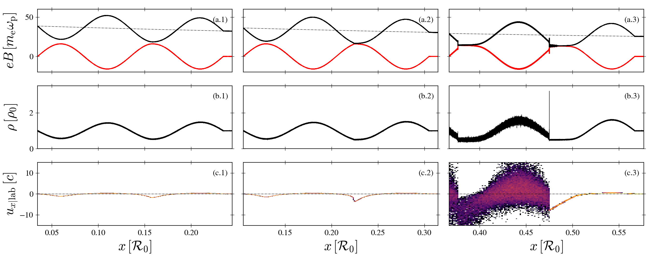
Figure 1 illustrates the propagation in the laminar (left), steepening (middle), and shock wave (right) regimes along the gradient. We observe the onset of strong steepening around . In the steepening region where [panel (a.2)], the flow accelerates up to relativistic speeds [panel (c.2)]. The wave then breaks, forming a shock, at , corresponding to about 2.25 wavelengths from the injection point. A second shock subsequently forms [Fig. 1(a-b.3)]. The shock forms near the wave trough, as expected from the analytic derivation in the appendix. Panels 1(a-b.3) also reveal a soliton structure, further detailed below, characterized by a sharp peak in density and electromagnetic field at the shock and associated with significant bulk flow heating. A careful examination indicates that the value of the compression factor at wave breaking is , corresponding to a plasma 4-velocity of . The corresponding value of the invariant at this location is . These values are in good agreement with the analytic results derived in the appendix, but note that the density profile adopted there differs from the one employed in the simulations. Following shock formation, the wave develops a plateau at phases where . This is clearly seen in Fig. 1(a.3). This plateau extends in size over time until complete eradication of the lower part of the wave. The corresponding wave energy is dissipated at the shock. The plasma in the plateau accelerates towards the shock before crossing it, while the magnetization decreases [see Fig. 1(c.3)]. The Lorentz factor just upstream of the shock increases as the wave evolves, reaching a maximum towards the end of the simulations, and then starts declining.
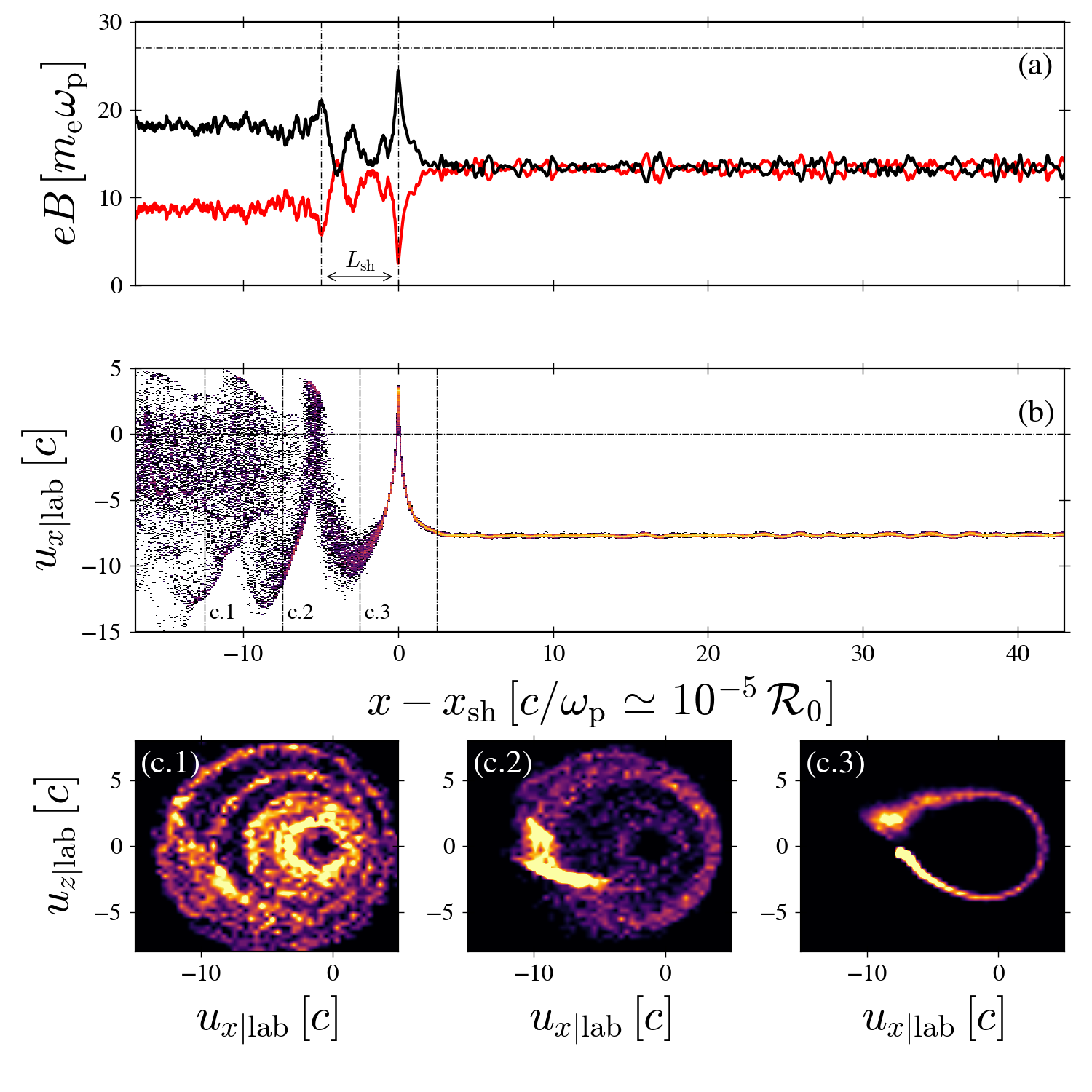
Figure 1 also reveals the generation of high-frequency precursor waves, likely formed by a synchrotron maser [21, 22, 23, 24, 25, 26, 27]. It is seen only in the leading shock, at in Fig. 1(c.1-3). The reason why the trailing shock does not generate a precursor wave is the high temperature of the upstream plasma caused by the passage of the leading shock (see panel c.3 in Fig. 1); the synchrotron maser operates efficiently only when the thermal spread of emitting particles is sufficiently small [28]. We emphasize that under realistic conditions, fast cooling of the shocked plasma, which can change the conditions at the trailing shock, is anticipated [5] but ignored in the present analysis. To elucidate the basic features of the shock structure and the precursor wave, we present in Fig. 2 an enlarged view of the immediate shock vicinity. We identify a (double) soliton-like structure [29], where the particle distribution forms a semicoherent cold ring in momentum space (see c.3 in the bottom panel of Fig. 2). A similar structure has been reported earlier for infinite planar shocks [27]. The precursor wave is dominated by a linearly polarized X-mode that propagates superluminaly against the upstream plasma. We also identified a precursor O-mode (Fig. 3), which is considerably weaker than the X-mode and seems unimportant.
The spectrum of the precursor wave (Fig 3), as measured in the Lab frame, exhibits several sharp harmonic peaks around , where denotes the proper plasma frequency, measured in the local rest frame of the fluid in the immediate upstream of the double soliton structure. These peaks correspond to the lowest harmonics of the resonant cavity defined by the double soliton structure seen in Fig. 2. In good agreement with [27], the wavelength of the highest peak and the width of the cavity are proportional, , with a weak dependence of on the upstream magnetization, . This implies that the peak frequency, as measured in the Lab frame, should scale as the shock Lorentz factor with respect to the Lab frame, (see appendix). From our simulations we estimate for the highest peak. Above the peak, the spectrum extends up to about . Below the peak, it cuts off at a frequency below which the wave is trapped by the shock (that is, the group velocity is smaller than the shock velocity). The latter can be estimated most easily in the rest frame of the upstream plasma. In this frame, the dispersion relation can be written as [30],
| (6) |
where is the cyclotron frequency. Upon transforming to the Lab frame, the dispersion relation reduces to in the limit (see appendix). The cutoff frequency and k-vector are obtained by equating the group velocity, , with the shock velocity with respect to the Lab frame, :
| (7) |
From the analysis of the data presented in Fig 2 we estimate and , from which we obtain upon transforming to the Lab frame. The cutoff frequency and k-vector given in Eq. (7) are in good agreement with those seen in Fig 3.
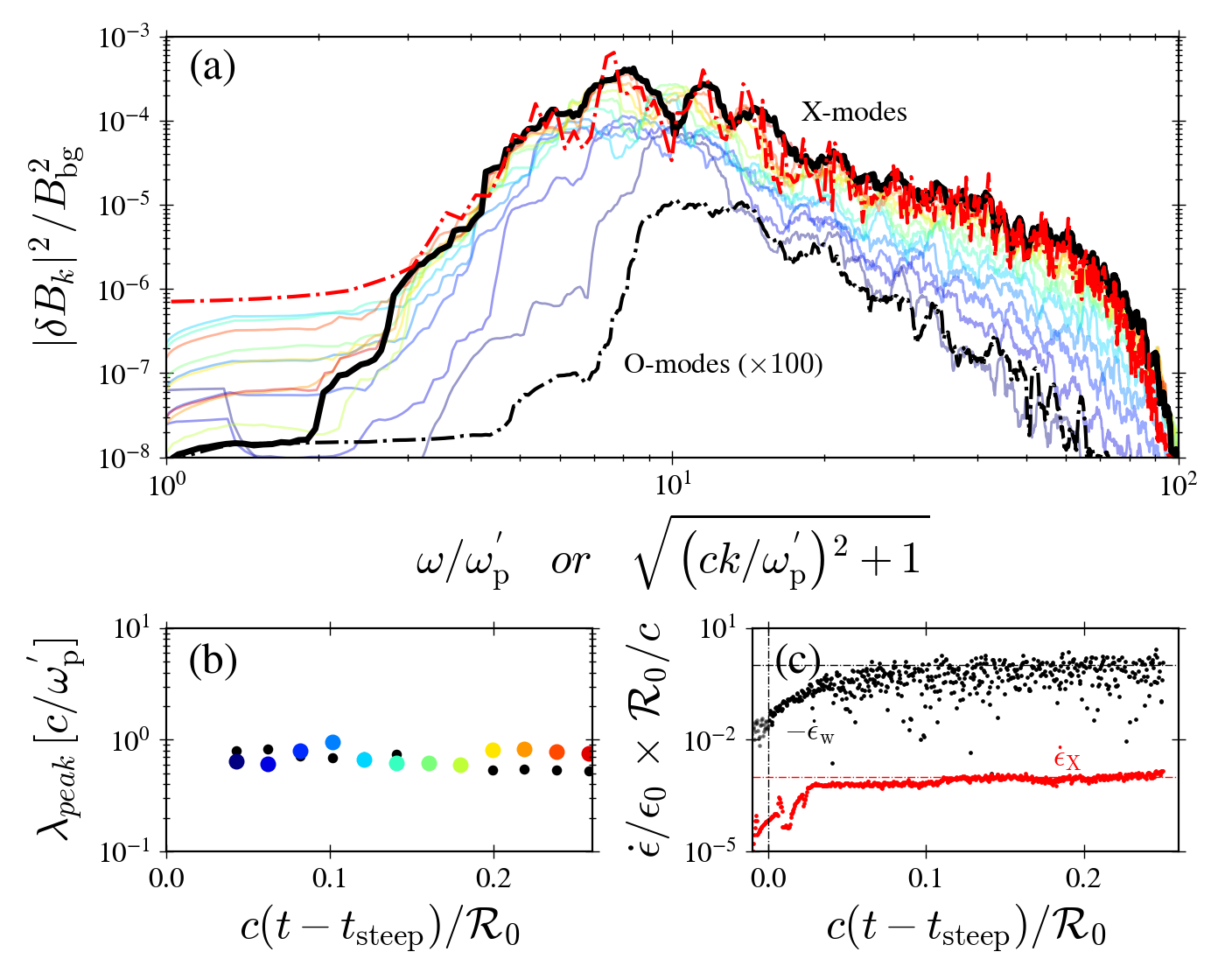
Regarding the efficiency of the precursor wave, we find that the X-mode carries a fraction of about of the total energy dissipated in the shock (the bottom half wave; see Fig. 3). As found in [27], the fraction of incoming kinetic energy converted into precursor waves in the post-shock frame is independent of the magnetization in the limit of . The increase in efficiency by a factor of unity () is consistent with the increase in downstream frame incoming particle kinetic energy across the simulation. We thus anticipate to be weakly sensitive to the conditions prevailing in the medium in which the FMS wave propagates.
We now consider a wave with luminosity erg/s, generated near the surface of a magnetar, and assume for simplicity that the wave propagates in the equatorial plane of the dipole background field, where G; cm being the stellar radius. The background density depends on the pair multiplicity in the magnetosphere, which is uncertain but expected to be large [31]; we henceforth adopt . With this normalization, the background number density, , can be expressed as cm-3, where is the angular velocity of the star, measured in rad/s, and is the Goldreich–Julian density. The corresponding plasma frequency of the background pair plasma is Hz.
The wave propagates nearly undisturbed in the magnetosphere until reaching a radius at which the wave breaks. This happens when , or cm. As discussed above, a shock forms and continues evolving with the wave. It can be shown [5] that the Lorentz factor just upstream of the shock quickly reaches a maximum value, and then gradually declines, roughly as up to , where the lower half of the wave is completely erased. The majority of the dissipated energy will be released in the -ray and -ray bands, and a fraction of in the form of a precursor wave. For our choice of parameters, and wave frequency Hz, . The upstream magnetization reaches a minimum, , and only slightly increases thereafter [5]. The proper plasma frequency in the shock upstream satisfies Hz, and barely changes in the wave dissipation zone, . Adopting the scaling we find from the simulations, , we anticipate the observed spectrum of the precursor wave to appear in the GHz band, as seen in many fast radio bursts.
Whether the precursor wave can escape the inner magnetosphere is unclear at present. It has been argued that GHz waves will be strongly damped in the inner magnetosphere by nonlinear decay into Alfvén waves [32], steepening or kinetic effects [33] (but cf. [34]). We note, however, that in the dissipation zone, where the precursor wave is formed, the peak frequency of the precursor wave is smaller than the background frequency by a factor a few, so the wave transitions from the MHD to the kinetic regime. Thus, the damping mechanisms mentioned above need to be reassessed. Moreover, the precursor wave is trapped by the kHz FMS wave, and the effect this has on the damping of the precursor wave needs to be studied. Finally, it has been shown [5] that under magnetar conditions, the cooling rate of the upstream plasma entering the shock is comparable to or even shorter than the Larmor frequency. How this might affect the efficiency of the precursor wave has yet to be determined.
In summary, we have demonstrated the self-consistent steepening, monster shock formation, and precursor wave emission emerging from a fast magnetosonic wave propagating along a declining background magnetic field. The analytical properties of wave steepening are found to be in good agreement with ab initio fully kinetic simulations. The ensuing shock formation leads to efficient dissipation of the bottom part of the wave over the dynamical time of the wave crossing. A fraction of about of the total dissipated energy is imparted to X-modes. The associated spectrum propagating upstream shows pronounced peaks corresponding to harmonics of the cavity forming between two leading solitons at the shock front. Finally, our results open promising avenues to study the fate of electromagnetic pulses propagating in strongly magnetized environments to address self-consistently their dissipation and, if any, the escaping signal.
Acknowledgements.
Acknowledgments This work was supported by a grant from the Simons Foundation (MPS-EECS-00001470-04) to AL. This work was facilitated by the Multimessenger Plasma Physics Center (MPPC, NSF grant PHY-2206607). The presented numerical simulations were conducted on the STELLAR cluster (Princeton Research Computing). This work was also granted access to the HPC resources of TGCC/CCRT under the allocation 2024-A0160415130 made by GENCI.Appendix A Appendix
Appendix B Exact solution for a 1D fast magnetosonic wave
Consider a FMS wave propagating in the positive direction is a scalar potential background magnetic field of the form , such that in the plane , so that . Since , . The wave fields are denoted by , . The equations governing the dynamics of the wave are derived using the general form of the stress-energy tensor:
| (8) |
where is the pressure, the specific enthalpy, and , here denotes the dual electromagnetic tensor. In terms of and it can be expressed as:
| (9) |
The homogeneous Maxwell’s equations read in this notation:
| (10) |
subject to . For the FMS wave under consideration , and , where is the component of the total magnetic field, as measured in the fluid rest frame. In the Lab frame . From Eq. (9) we find
| (11) |
here is the wave electric field.
Denote for short and , where is the enthalpy per particle, the component of Equation (10) combined with the continuity equation, (assuming no particle creation), yields: . Thus, is conserved along streamlines. We choose an equation of state of the form for adiabatic index . Then
| (12) |
Using the equation , the relation , and the continuity equation, one finds:
| (13) | |||
| (14) |
here is the convective derivative, and . The fast magnetosonic speed is defined by
| (15) |
For a cold plasma, , it reduces to
| (16) |
where
| (17) |
is the magnetization of the fluid. In terms of the variable , Eqs. (13) and (14) can be rewritten in the form
| (18) | |||||
| (19) |
where the relations , , and have been employed. Further manipulation of the latter equations yields
| (20) |
here
| (21) |
are the Riemann invariants of the system, and
| (22) |
are the velocities of the characteristics on which propagate, as measured in the Lab frame.
Consider now a wave injected at time from a source located at and moving rightward. Since ahead of the wave , and the background field is independent of time, satisfies
| (23) |
where . To order the solution is , here is the background magnetic field at the source. Then, , and Eq. (20) for reduces to
| (24) |
To find , we use the relations (Eq. 15), suitable for cold plasma, and . Integrating from to , one obtains
| (25) | |||||
| (26) |
where the constant is determined from the condition : . Note that implies and , hence, the magnetic field equals the background field. The magnetization can be readily computed using Eq. (16): . From this, one finds:
| (27) |
With the above results, the right-hand side of Eq. (24) can be expressed as a function of . Let us denote for short . The evolution of along the characteristic is governed by the coupled ODEs
| (28) | |||||
| (29) |
subject to the boundary conditions , , here is a specified injection function. In case of a uniform field, , is conserved along and the solution can be expressed as , with given implicitely by
| (30) |
Realistic magnetospheres are nearly force-free, that is, . In this limit, we can expand and to obtain a more convenient set of equations. In terms of we obtain:
| (31) |
We consider background magnetic field profiles of the form , with and chosen in the simulations presented in the main part. For convenience and without loss of generality, we choose the origin to be located at , and normalize time and length to ; , . Equations (28) and (29) then take the form:
| (32) | |||||
| (33) |
To find , note that since const, , from which one obtains:
| (34) |
The solution is
| (35) |
where , and . The magnetization of the plasma is given by (Eq. 27). It declines monotonically with as the wave propagates. The solution for is obtained now using :
| (36) |
Substituting and into Eq. (32) yields
| (37) |
The solution can be expressed as
| (38) |
This solution can be inverted to yield . Substituting into Eq.(36) yields the trajectory of the characteristic, , that satisfies . The family of all characteristics is labeled by the injection time . It can be expressed as , with . The injection function gives the corresponding values of at . For injection of a periodic wave at the boundary (), with electric field , Eqs. (11) and (27) yield:
| (39) |
Crossing of characteristics is determined from the condition , where the partial derivative is taken at a constant time . However, this equation admits multiple solutions. A shock will initially form at the first crossing, that is, at the earliest time, defined by . The solution of the two equations above yields a unique value, , from which the location and time of shock formation can be computed. The plasma 4-velocity at this location is given by .
For illustration, consider . For this choice Eq. (38) can be readily integrated, yielding
| (40) |
where
| (41) |
To estimate the location of the caustic (if exists) for a characteristic with initial value we use Eq. (36) to obtain . Assuming , one finds:
| (42) |
here denotes the value of at the caustic for the characteristic . Now, for a typical case we anticipate and . In addition, since the caustic occurs near the turnaround point, , at which (see Eqs. 31 and 35), we anticipate . Expanding in powers of and , we find
| (43) |
The shock first appears at the earliest crossing, that is, at for which is a minimum. Differentiating Eq. (43) at a constant , and substituting from Eq. (42), gives
| (44) |
using , . Comparing Eq. (44) with Eq. (42), we obtain the compression factor,
| (45) |
and the time of shock birth:
| (46) |
The corresponding plasma 4-velocity is , here (see Eq. 35). The magnetization of the flow at this location is .
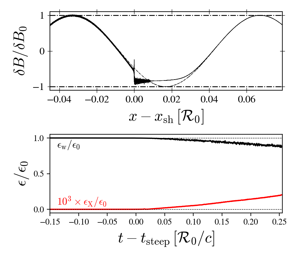
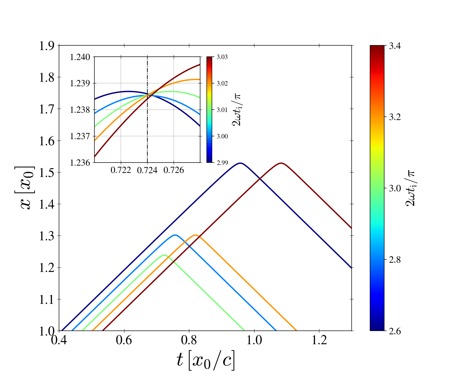
Figure 4 exhibits sample characteristics computed from Eqs. (36) and (40) for , , , and , injected at the indicated times (around the wave trough). As seen, each characteristic turns around at , at which changes sign (Eq. 31). The inset shows a zoom-in around the location of shock birth; it indicates , , . These values are in excellent agreement with the above estimates ( from Eqs. 45, from Eq. 46 and ). In units of the wavelength we have: . The corresponding plasma 4-velocity is . These numbers are in rough agreement with the simulations, although we stress that the comparison is not perfect since, in the simulations, we adopt a constant density for numerical convenience rather than invoking const.
Once the shock forms, it gradually grows in strength as the plasma upstream of the shock continues accelerating towards the source (since declines). To compute the shock velocity, we use the jump conditions of a strongly magnetized shock. Since the magnetization of the upstream plasma is large, , here and is the initial value of the characteristic that crosses the shock from the upstream. In this limit, the velocity of the downstream flow, as measured in the shock frame, is , where, henceforth, prime denotes quantities measured in the shock frame. Mass conservation implies . Using Eq. (27), one finds . Transforming to the Lab frame we obtain: , where . Combining the above results yields the shock velocity in the Lab frame:
| (47) |
noting that . Thus, it is seen that the shock propagates in the positive direction, that is, opposite to the direction of plasma motion. To find the evolution of the wave subsequent to shock formation, one needs to solve the characteristics equations, Eqs. (28)-(29), coupled to the equation of the shock trajectory, . We shall not present such analysis here. Instead, the shock structure and propagation are illustrated in Fig. 5 from the kinetic simulations. As the main text explains, we launch a periodic FMS wave from , letting it propagate along in a cold pair plasma with a declining background magnetic field, constant density, and large initial background magnetization. The weakly declining background magnetic field is set to be static and external for convenience. The top panel shows a comparison between the wave profile after and before saturation. A kinetic scale fluid discontinuity, a shock, is visible at . The time evolution of the power of the ensuing wave propagating upstream of the shock, dominated by X-modes, is illustrated in the bottom panel.
Appendix C Dispersion relations
In the rest frame of the fluid, the dispersion relations of the precursor wave read:
| (48) |
where is the proper plasma frequency, and . Transforming to the laboratory frame, one obtains,
| (49) | |||||
| (50) |
Inverting the transformation and using Eq. (48), yields:
| (51) |
Noting that , we deduce that for , , so that to a good approximation . The group velocity in the Lab frame can be readily computed now:
| (52) |
The wave will be trapped by the shock if , or
| (53) |
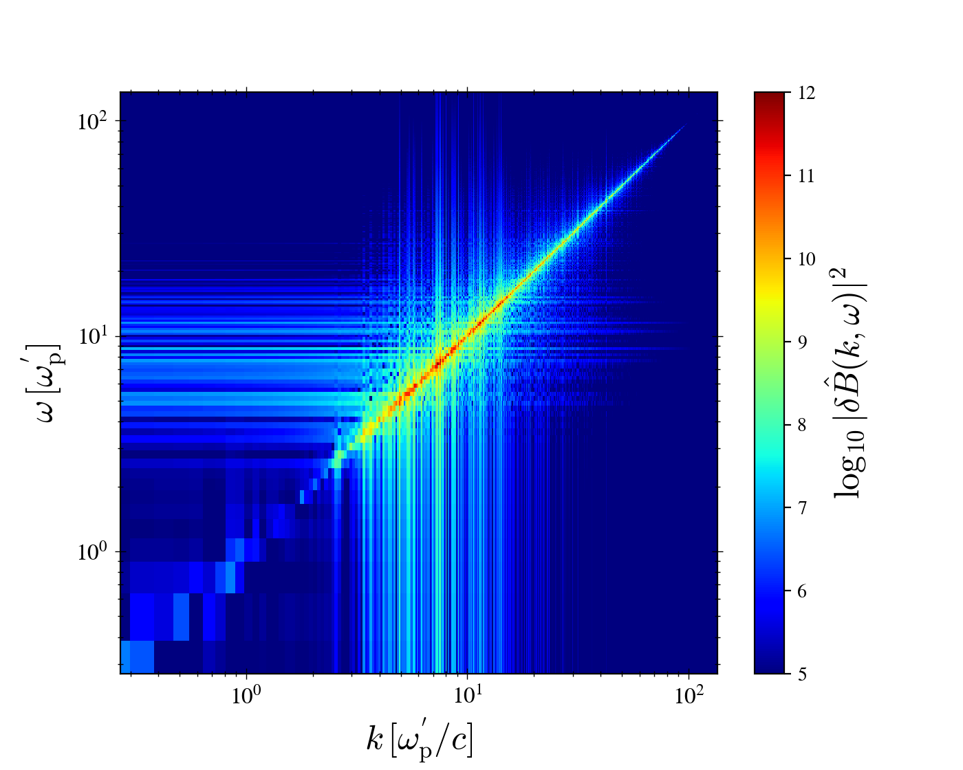
Figure 6 shows the dispersion relation of the X-modes in the immediate shock upstream, obtained from the simulations, in units of . We notice that the branch closely corresponds to light modes, as expected from Eq. (52), and that the shock imposes a low frequency/wavelength cutoff, in agreement with Eq. (53). Note that the dispersion relation is computed in the laboratory frame and not in the upstream frame, as in Eq. (48).
References
- Thompson and Duncan [1995] C. Thompson and R. C. Duncan, Mon. Not. Roy. Astron. Soc. 275, 255 (1995).
- Parfrey et al. [2013] K. Parfrey, A. M. Beloborodov, and L. Hui, Astroph. J. 774, 92 (2013), arXiv:1306.4335 [astro-ph.HE] .
- Chen et al. [2022] A. Y. Chen, Y. Yuan, X. Li, and J. F. Mahlmann, arXiv e-prints , arXiv:2210.13506 (2022), arXiv:2210.13506 [astro-ph.HE] .
- Yuan et al. [2022] Y. Yuan, A. M. Beloborodov, A. Y. Chen, Y. Levin, E. R. Most, and A. A. Philippov, Astroph. J. 933, 174 (2022), arXiv:2204.08513 [astro-ph.HE] .
- Beloborodov [2023a] A. M. Beloborodov, Astroph. J. 959, 34 (2023a), arXiv:2210.13509 [astro-ph.HE] .
- Mahlmann et al. [2023] J. F. Mahlmann, A. A. Philippov, V. Mewes, B. Ripperda, E. R. Most, and L. Sironi, Astroph. J. Lett. 947, L34 (2023), arXiv:2302.07273 [astro-ph.HE] .
- Lyubarsky [2014] Y. Lyubarsky, Mon. Not. Roy. Astron. Soc. 442, L9 (2014), arXiv:1401.6674 [astro-ph.HE] .
- Lyutikov et al. [2016] M. Lyutikov, L. Burzawa, and S. B. Popov, Mon. Not. Roy. Astron. Soc. 462, 941 (2016), arXiv:1603.02891 [astro-ph.HE] .
- Waxman [2017] E. Waxman, Astroph. J. 842, 34 (2017), arXiv:1703.06723 [astro-ph.HE] .
- Lyubarsky [2021] Y. Lyubarsky, Universe 7, 56 (2021), arXiv:2103.00470 [astro-ph.HE] .
- Mahlmann et al. [2022] J. F. Mahlmann, A. A. Philippov, A. Levinson, A. Spitkovsky, and H. Hakobyan, Astroph. J. Lett. 932, L20 (2022), arXiv:2203.04320 [astro-ph.HE] .
- Thompson [2023] C. Thompson, Mon. Not. Roy. Astron. Soc. 519, 497 (2023), arXiv:2209.11136 [astro-ph.HE] .
- Most et al. [2024] E. R. Most, A. M. Beloborodov, and B. Ripperda, arXiv e-prints , arXiv:2404.01456 (2024).
- Lyubarsky [2020] Y. Lyubarsky, Astroph. J. 897, 1 (2020), arXiv:2001.02007 [astro-ph.HE] .
- Metzger et al. [2019] B. D. Metzger, B. Margalit, and L. Sironi, Mon. Not. Roy. Astron. Soc. 485, 4091 (2019), arXiv:1902.01866 [astro-ph.HE] .
- Khangulyan et al. [2022] D. Khangulyan, M. V. Barkov, and S. B. Popov, Astroph. J. 927, 2 (2022), arXiv:2106.09858 [astro-ph.HE] .
- Ripperda et al. [2022] B. Ripperda, M. Liska, K. Chatterjee, G. Musoke, A. A. Philippov, S. B. Markoff, A. Tchekhovskoy, and Z. Younsi, Astroph. J. Lett. 924, L32 (2022), arXiv:2109.15115 [astro-ph.HE] .
- Mahlmann et al. [2020] J. F. Mahlmann, A. Levinson, and M. A. Aloy, Month. Not. Roy. Astron. Soc. 494, 4203 (2020), arXiv:2001.03171 [astro-ph.HE] .
- Chashkina et al. [2021] A. Chashkina, O. Bromberg, and A. Levinson, Month. Not. Roy. Astron. Soc. 508, 1241 (2021), arXiv:2106.15738 [astro-ph.HE] .
- Hakobyan et al. [2023] H. Hakobyan, A. Spitkovsky, A. Chernoglazov, A. Philippov, D. Groselj, and J. Mahlmann, Princetonuniversity/tristan-mp-v2: v2.6 (2023).
- Sazonov [1973] V. N. Sazonov, Soviet Astronomy 16, 971 (1973).
- Hoshino et al. [1992] M. Hoshino, J. Arons, Y. A. Gallant, and A. B. Langdon, Astrophys. J. 390, 454 (1992).
- Gallant et al. [1992] Y. A. Gallant, M. Hoshino, A. B. Langdon, J. Arons, and C. E. Max, Astrophys. J. 391, 73 (1992).
- Lyubarsky [2006] Y. Lyubarsky, Astroph. J. 652, 1297 (2006), arXiv:astro-ph/0611015 [astro-ph] .
- Iwamoto et al. [2017] M. Iwamoto, T. Amano, M. Hoshino, and Y. Matsumoto, Astroph. J. 840, 52 (2017), arXiv:1704.04411 [astro-ph.HE] .
- Iwamoto et al. [2018] M. Iwamoto, T. Amano, M. Hoshino, and Y. Matsumoto, Astroph. J. 858, 93 (2018), arXiv:1803.10027 [astro-ph.HE] .
- Plotnikov and Sironi [2019] I. Plotnikov and L. Sironi, Mon. Not. Roy. Astron. Soc. 485, 3816 (2019), arXiv:1901.01029 [astro-ph.HE] .
- Babul and Sironi [2020] A.-N. Babul and L. Sironi, Mon. Not. Roy. Astron. Soc. 499, 2884 (2020), arXiv:2006.03081 [astro-ph.HE] .
- Alsop and Arons [1988] D. Alsop and J. Arons, Phys. Fl. 31, 839 (1988).
- Hoshino and Arons [1991] M. Hoshino and J. Arons, Physics of Fluids B 3, 818 (1991).
- Beloborodov [2021] A. M. Beloborodov, Astroph. J. Lett. 922, L7 (2021), arXiv:2108.07881 [astro-ph.HE] .
- Golbraikh and Lyubarsky [2023] E. Golbraikh and Y. Lyubarsky, Astroph. J. 957, 102 (2023), arXiv:2309.09218 [astro-ph.HE] .
- Beloborodov [2023b] A. M. Beloborodov, arXiv e-prints , arXiv:2307.12182 (2023b), arXiv:2307.12182 [astro-ph.HE] .
- Lyutikov [2023] M. Lyutikov, arXiv e-prints , arXiv:2310.01177 (2023), arXiv:2310.01177 [astro-ph.HE] .