Fast-oscillating random perturbations of Hamiltonian systems
Abstract
We consider coupled slow-fast stochastic processes, where the averaged slow motion is given by a two-dimensional Hamiltonian system with multiple critical points. On a proper time scale, the evolution of the first integral converges to a diffusion process on the corresponding Reeb graph, with certain gluing conditions specified at the interior vertices, as in the case of additive white noise perturbations of Hamiltonian systems considered by M. Freidlin and A. Wentzell.
The current paper provides the first result where the motion on a graph and the corresponding gluing conditions appear due to the averaging of a slow-fast system, with a Hamiltonian structure, on a large time scale.
The result allows one to consider, for instance, long-time diffusion approximation for an oscillator with a potential with more than one well.
Keywords: Averaging, slow-fast system, gluing conditions, diffusion approximation
Mathematics Subject Classification: 37J40, 60F17
1 Introduction
Consider a family of diffusion processes in satisfying
| (1.1) | ||||
where is a small positive parameter, is the -dimensional torus, and is an -dimensional Brownian motion. In the coupled slow-fast system, is the slow component and is the fast component, since the generator of the diffusion in the second equation is multiplied by . On the space , the diffusion (1.1) is everywhere degenerate. All the randomness comes from the second equation and is transmitted to through the vector , which is fast-oscillating in time. Under natural conditions, the averaging principle holds for the process in (1.1) (cf. [11]). For example, if is non-degenerate (and thus has a unique invariant measure independent of ), then converges as in probability on each finite interval to an averaged process defined by the differential equation
| (1.2) |
where . Therefore, can be viewed as a result of fast-oscillating random perturbations, i.e. , of the deterministic process . Moreover, the deviation can be described more precisely: the process converges weakly to a Gaussian Markov process on a finite interval (cf. [14], [2]), and, if we assume a special type of vector , then the local limit theorem holds for at time ([16]).
If the system (1.2) has a first integral , then, by the averaging principle, is nearly constant on finite time intervals when is small. Nontrivial behavior can, however, be observed on larger time intervals (of order ). Assume, momentarily, that has a single critical point. Then it was demonstrated in [3] that converges weakly in , as , to a diffusion process for any finite , under additional assumptions. A similar result in the case of multiple degrees of freedom was obtained recently in [9] and the main goal there was to overcome difficulties related to resonances, which is typical in the case of multiple degrees of freedom. The result holds in the region where no critical points of the first integrals are present and action-angle-type coordinates can be introduced.
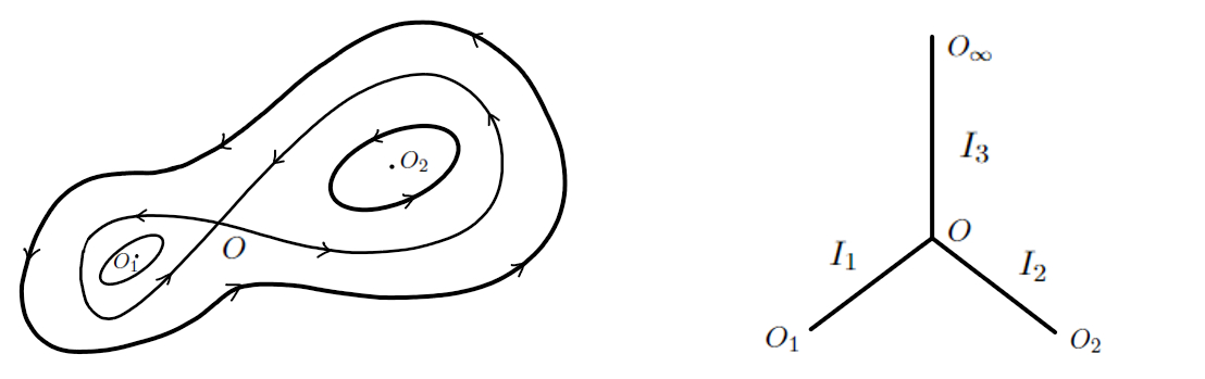
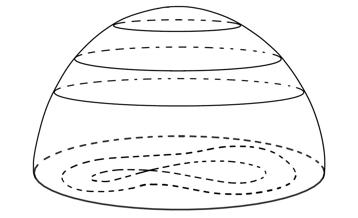
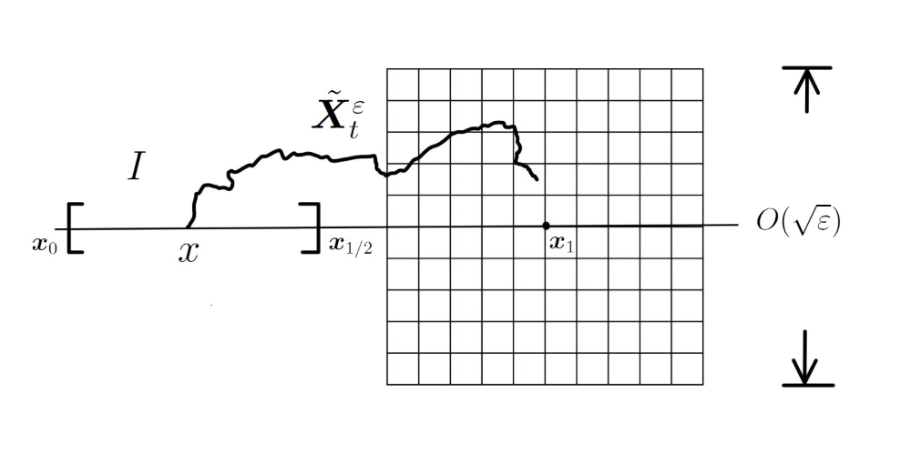
Let us return to the two-dimensional situation. In the presence of multiple critical points, including saddle points, the problem gets more complicated as we need to consider the Reeb graph in order to describe the evolution of the first integrals denoted by , where the additional discrete-valued first integral is the label of the edge on the Reeb graph. (For instance, in Figure 1, we have one saddle point and two local minima of in the space . Accordingly, on the graph, we have one interior vertex, three exterior vertices, including one formally representing the infinity, and three edges connecting them.) In particular, the interior vertices on the graph correspond to the level curves that contain the saddle points, and those level curves are called the separatrices. In this situation, the limiting behavior has already been described for the white-noise-type additive perturbations of dynamical systems: Hamiltonian systems in ([12]), general dynamical systems with conservation laws in ([10]), and Hamiltonian systems with an ergodic component on two-dimensional surfaces ([5],[6],[4]).
In this article, we consider fast-oscillating random perturbations, as discussed above, of Hamiltonian system in with multiple critical points and prove that the evolution of the first integrals converges to a diffusion process defined by an operator ( on the corresponding Reeb graph. In particular, the exterior vertices turn out to be inaccessible and the behavior of the process near the interior vertices is described in terms of the domain in the following way: for interior vertex , there are constants such that each function satisfies
| (1.3) |
where means that is an endpoint of . Intuitively, the absolute value of is proportional to the probability of entering edge after the process arrives at the vertex . The relation (1.3) is usually referred to as the gluing condition. In the next section, we will formulate the results along with the assumptions more precisely. The coefficients will be calculated explicitly. As we mentioned, similar results hold in case of additive perturbations of Hamiltionian systems. Now the techniques in the proof are more involved and require new ideas with analysis on multiple time scales : , , , etc. It is worth noting that our result provides the first example where the motion on a graph and the corresponding gluing conditions appear as a result of averaging of a slow-fast system, with a Hamiltonian structure, on a large time scale.
In the remainder of this section, we briefly introduce the main idea and the critical steps of the proof, and outline the plan of the paper. To start with, since our interest is in the long-time behavior of on time scales, it is often convenient to consider a temporally re-scaled process :
| (1.4) | ||||
It is clear that in distribution. Thus, it suffices to prove the weak convergence of in the space , where is the Reeb graph. The proof of the weak convergence relies on demonstrating that the pre-limiting process asymptotically solves the martingale problem. Namely, we will show that, for each in a sufficiently large subset of and ,
| (1.5) |
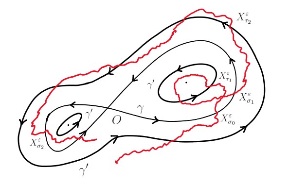
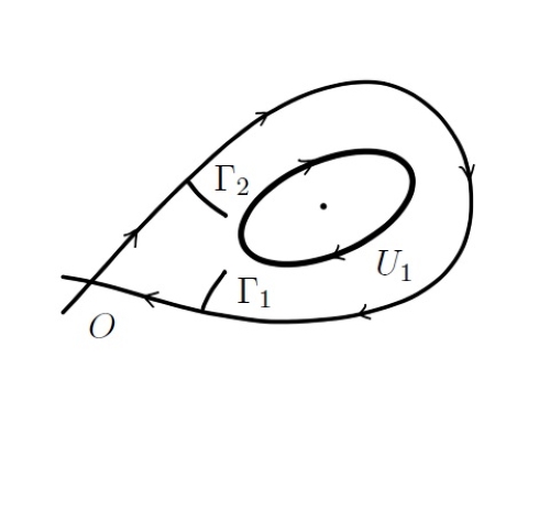
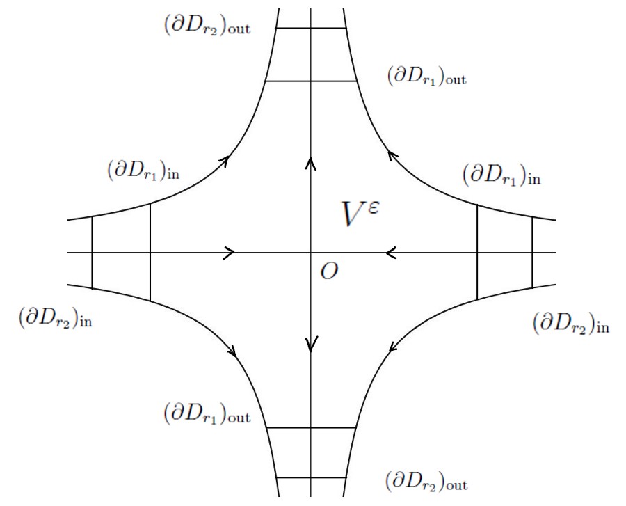
as , uniformly in in any compact set in and in . Note that, contrary to the standard formulation of the martingale problem, there is no conditioning in (1.5). However, (1.5) is still enough for our purpose (see Lemma 2.4), since is a family of strong Markov processes. The main idea in our proof of (1.5) is to divide the time interval into excursions between different visits to the separatrices and show that the contribution from each excursion is small and they do not accumulate. For example, suppose for now that there is only one saddle point, as shown in Figure 2. Let be the saddle point with , be the separatrix, be a set near the separatrix, where , and be the first time when the process reaches . Define inductively the two sequences of stopping times:
| (1.6) | ||||
and consequently two Markov chains and .
As pointed out earlier, we wish to prove that the contributions to (1.5) from all individual excursions are small and the sum converges to zero as . Thus, except for the first and the last excursions, it is sufficient to show that (a) the expectation corresponding to one excursion converges to zero as uniformly in initial distribution, (b) the expectation corresponding to one excursion is exactly zero, for all , if the process starts with the invariant measure of the Markov chain on , and (c) the measures on induced by converge exponentially, as , uniformly in and in initial distribution, to the invariant one.
The claim in (a) is an extension of the results outside of the singularities in [9], and new difficulties arise due to the degenerations occurring on the boundaries. The claim in (b) is true if there is a common invariant measure for the processes for all and the gluing conditions are chosen appropriately. In general, there is no common invariant measure for all , and we need to consider a family of auxiliary processes that do have a common invariant measure, and then use the proximity of the auxiliary and the original processes near the separatrix, and the Girsanov theorem to show that the gluing conditions are actually the same. The assertion in (c) is hard to verify, and its proof requires new techniques, including a local limit theorem for time-inhomogeneous functions of Markov processes and density estimates for hypoelliptic diffusions that will be discussed in later sections.
Plan of the paper.
In Section 2, we introduce the notation, state the assumptions, formulate the main result and the lemma we use to establish the weak convergence. In Section 3, the problem is reduced to the case we discussed where there is only one saddle point. Besides, we construct an auxiliary process with -independent invariant measure and derive diffusion approximations of the processes. In Section 4, we prove the averaging principle for the process on the Reeb graph up to the time when the process reaches an interior vertex. In Section 5, we construct the Markov chain on the product space of the separatrix and the -torus (see (1.6)) and prove its convergence to the invariant measure with an exponential rate uniformly in . In Section 6, we prove the main result. A few technical results including time estimates near the vertices and tightness of the processes are included in the Appendix.
2 Main result
Throughout this article, and represent the probability and expectation, respectively, and the subscripts pertain to initial conditions.
denotes the natural filtration generated by the process .
For brevity, the stopping times’ dependence on parameters and initial conditions is not always indicated in the notation when introduced (e.g. (1.6)). denotes a first order differential operator, i.e., derivative, gradient, Jacobian, etc., depending on the context.
denotes the indicator function of the event .
If and are two non-negative functions that depend on an asymptotic parameter, we write if .
is the space of continuous functions on the Reeb graph that tend to zero at infinity with uniform norm.
is the projection onto .
In order to formulate the assumptions and results, we further introduce the following notation.
Notation.
-
(i)
’s are the vertices on the graph and are occasionally used to denote the corresponding critical points on the plane when there is no ambiguity. ’s are the edges on the graph and ’s are the corresponding two-dimensional domains. Formally, is the vertex that corresponds to infinity. A symbol between a vertex and an edge means that the vertex is an endpoint of the edge.
-
(ii)
Consider the following metric on : is the length of the shortest path connecting and . For example, if , , , , and , then .
-
(iii)
and is the connected component of in the domain .
-
(iv)
.
-
(v)
is the diffusion process on with the generator , where
(2.1) -
(vi)
For in the interior of , define
(2.2)
The following conditions are assumed to hold throughout the article.
Assumptions.
-
(H1)
and are functions on . is matrix-valued and is positive-definite for all .
-
(H2)
is a function from to with bounded second derivatives. has a finite number of non-degenerate critical points. Each level curve corresponding to a vertex on the Reeb graph contains at most one critical point. As , .
-
(H3)
is a function from to such that the averaged process is a Hamiltonian system with , i.e. .
-
(H4)
The fast-oscillating perturbation is non-degenerate, i.e. spans for each , and is uniformly bounded together with its first derivatives.
-
(H5)
For each that belongs to one of the separatrices, there exists such that the process in (1.1) satisfies the parabolic Hörmander condition at . Namely, with being the drift term in the equation for in the Stratonovich form, we have that
(2.3) at spans , where is the -th column of , is the Lie bracket, and Lie is the Lie algebra generated by a set (cf. [13] or Section 2.3.2 of [17]).
Definition 2.1.
The domain consists of functions satisfying:
-
(i)
is twice continuously differentiable in the interior of each edge of ;
-
(ii)
The limits exist and do not depend on the edge ;
-
(iii)
For interior vertex , there are constants such that
(2.4)
where the sign is taken if is minimum on , and the sign is taken otherwise. The operator on the Reeb graph is defined by
| (2.5) |
for and in the interior of , and defined as at the vertex .
By the Hille-Yosida theorem (see, for example, Theorem 4.2.2 in [7]), one can check that there exists a unique strong Markov process on with continuous sample paths that has as its generator. Now we are ready to formulate the main result of this article.
Theorem 2.2.
Remark 2.3.
The last condition in (H2) can be relaxed without much extra effort since the limiting process defined by cannot reach infinity in finite time. In addition, as seen from the proofs in Section 5 and Remark 5.7, assumption (H5) can be relaxed so that it holds for at least one point on each separatrix. Moreover, if the number of Lie brackets needed to generate in the parabolic Hörmander condition is assumed to be given, then we can relax the assumptions on smoothness of the coefficients.
To prove the theorem, we need a result on weak convergence of processes, that is Lemma 4.1 in [8] adapted to our case (see also the original statement in [12]):
Lemma 2.4.
Let be a dense linear subspace of and be a linear subspace of , and suppose that and have the following properties:
-
(1)
There is a such that for each the equation has a solution ;
-
(2)
For each , each , and each compact ,
(2.6)
uniformly in and .
Suppose that, for each starting point of , the family of measures on induced by the processes , , is tight. Then, for each starting point of , converges weakly to the strong Markov process on the Reeb graph that has the generator and the initial distribution .
Here we choose to be all the functions in that are twice continuously differentiable in the interior of each edge; to be all the functions in that are four times continuously differentiable in the interior of each edge. It is easy to check condition holds in Lemma 2.4, and the tightness of distributions of , , is verified in Appendix C. Then the main ingredient of the proof is to verify (2.6) in condition (2) of Lemma 2.4.
3 Preliminaries
In this section, we explain some technical difficulties and our approach to the proof.
3.1 Localization
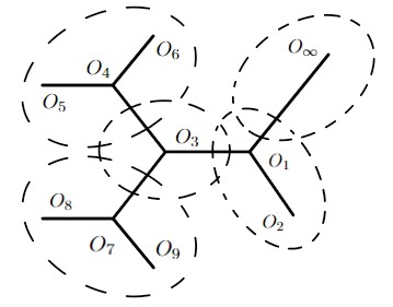
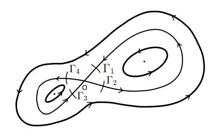
Considering Theorem 2.2 for in the state space causes technical difficulties due to the presence of multiple separatrices of the Hamiltonian and to the fact that the process is not positive recurrent. However, such difficulties can be circumvented by considering the process locally. Namely, let us cover the plane by finitely many bounded domains, each containing one of the separatrices and bounded by up to three connected components of level sets of , and one unbounded domain not containing any critical points. For example, as shown in Figure 3, we have different parts of the Reeb graph that correspond to the domains in . Every point of can be assumed to be contained in the interior either one or two domains. Since it takes positive time to travel from the boundary of one domain to the boundary of another, it suffices to prove the result up to time of exit from one domain. To be more precise, let be the open cover. Define and, for such that , define , . In order to prove (2.6), it suffices to prove instead, uniformly in in any compact set in and in , that
| (3.1) |
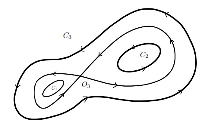
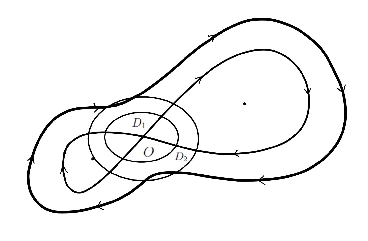
since it also implies that as , uniformly in all sufficiently small. In the unbounded domain without critical points, (3.1) can be obtained using the result in bounded domain together with the tightness of . It remains to consider the bounded domains. Let be one of the bounded domains. As explained below, the process in can be extended beyond the time when it reaches the boundary by embedding into a compact manifold with an area form and a Hamiltonian such that there are no other separatrices.
Consider the case where is not simply connected - for example, is the domain that contains in Figure 3. There are three connected components of as shown in Figure 4(a) (other situations can be treated similarly). Then we can modify the Hamiltonian and the vector field in and in such a way that assumptions (H2)-(H4) hold locally, and there is only one extremum point of in and one in (this modification is not needed if is simply connected). The unbounded domain outside can be replaced by a compact surface so that the resulting state space of is, topologically, a sphere . Then, the vector field on the surface can be chosen as a smooth extension from so that the averaged process is a Hamiltonian system on with respect to an area form , which is simply on , , and . Moreover, there exists a chart such that the corresponding vector field on satisfies that spans for each and the averaged process is a Hamiltonian system with respect to on . For example, as shown in Figure 4(b), we can modify the vector field on the plane outside so that there are two disks with the same center , and the averaged process is a Hamiltonian system in , in particular, rotation between and . Then is smoothly glued to a hemisphere and the resulting manifold is , and the vector field can be extended to the surface in such a way that the averaged process is a rotation with certain constant angular velocity on the level sets.
It is clear that, when restricted to , the resulting system defined on has exactly the same behavior as the original process on . Therefore, it suffices to prove (3.1) for the new process on . Let us formally restate the corresponding assumptions and formulate the result on . In the remainder of the paper, all the definitions (e.g. the quantities defined in Section 2) and statements on are understood by locally choosing coordinates so that . In particular, on , they are understood in the coordinate , while on the ”flat” part that contains , they are understood in the usual way. Then the assumptions on the coefficients on are analogous to those introduced earlier, so we only mention the differences:
From this point on, we denote the process on as , and on the time scale (defined by (1.1) and (1.4) with replaced by ), and assume that the conditions (H2′)-(H4′) replacing (H2)-(H4) hold. Then (2.6) follows from the next result (see (3.1)).
Proposition 3.1.
For each and each ,
| (3.2) |
as , uniformly in , , and that is a stopping time w.r.t. .
3.2 Auxiliary process
It turns out that similar results hold for a more general process with a slightly perturbed fast component:
| (3.3) | ||||
where is infinitely differentiable. Namely, converges weakly to the Markov process defined by the operator on the Reeb graph. Here, the subscript indicates that depends on the choice of . If , then it is clear that , and thus . However, if , then we have an additional drift term in (3.3), and thus we need an additional drift term in the generator of the limiting process. While a precise definition of is deferred to later sections, we observe that the operators replacing depend on , and the domain as well as the linear subspace, denoted by , chosen in Lemma 2.4 also vary for different . Therefore, in order to formulate general results, we consider , the set of continuous functions on that are four-times continuously differentiable inside each edge and satisfy conditions (i) and (iii) in Definition 2.1, as well as a weaker form of condition (ii), namely, the limits exist but are not necessarily independent of the edge . Note that contains for all choices of . Define on by applying the differential operator ( plus an additional drift corresponding to ) on each edge separately, with the result not being necessarily continuous at the interior vertices.
As mentioned before, we need to construct a family of auxiliary processes that, on the one hand, have a common invariant measure for all and, on the other hand, are close to the processes of interest. The auxiliary process on can in fact be obtained by choosing a special in (3.3). We denote this particular choice of as . Now we find such that is the invariant measure for the process with every , where is the area measure w.r.t. and is the invariant measure for in . Let be the generator of the process :
Hence, is the invariant measure if , where is the adjoint operator of and is the density of , i.e.
| (3.4) |
where is the adjoint operator of . Since is the invariant measure for , the last term vanishes. Hence (3.4) reduces to
| (3.5) |
To see the existence of the solution, we need the following lemma (cf. Lemma 2.1 in [9]).
Lemma 3.2.
Let be a bounded function on that is infinitely differentiable, and let be the generator of a non-degenerate diffusion on with the unique invariant measure and suppose that for each . Then there exists a unique solution to the equation
| (3.6) |
and is also bounded and infinitely differentiable. Moreover, if has uniformly bounded derivatives up to order in (or , the same holds for .
Remark 3.3.
As in (1.4), we define in distribution. Then, a simple corollary can be obtained by using Lemma 3.2 and then applying Ito’s formula to the corresponding solution and (cf. Lemma 2.3 in [9]).
Corollary 3.4.
Let satisfy the all the conditions in Lemma 3.2 with and , then for fixed
| (3.7) |
uniformly in , , and that is a stopping time bounded by .
3.3 Diffusion approximation
Since , by Lemma 3.2, there exists a function that is bounded together with its derivatives such that
| (3.8) |
The equation is understood element-wise. Apply Ito’s formula to :
| (3.9) | ||||
Combining (3.3), (3.8), and (3.9), we obtain
| (3.10) | ||||
Similarly, by applying Ito’s formula to and repeating the steps above, we have
| (3.11) | ||||
This idea of diffusion approximation is frequently used in the remainder of the paper, and the function always refers to the solution to (3.8).
4 Averaging principle inside one domain
In this section, we consider a general process defined after Remark 3.3, which is a faster version of the process in (3.3). The process takes values on . As a result of localization, is separated into three domains, each bounded by the separatrix or a part of it. This section is devoted to the proof of the averaging principle for on up to time when exits from one of the three domains. The domain under consideration will be denoted by . Therefore, without any ambiguity, the projection simply reduces to the Hamiltonian . Let be the region in between and , be the saddle point, and be the extremum point, and further define stopping times and . Without loss of generality, we assume that and .
4.1 Averaging principle before
We aim to prove the averaging principle between and with constants and . Notice that, for technical reasons, we assume that in this intermediate result and in the proofs that utilize it in this subsection and the next, while we always assume that elsewhere. Let us further define another coordinate inside this domain . Let denote the curve that is tangent to at each point and connects the saddle point and the extremum point , and let be the intersection of and . Let denote the time it takes for the averaged process to make one rotation on and denote the time it takes for starting from to arrive at . Now we define the coordinate whose range is . It is easy to see that has constant speed in coordinate. Since there is logarithmic delay near the saddle point, the coordinate has exploding derivatives near the separatrix. However, as shown in Appendix A, the order of its derivatives w.r.t. the Euclidean coordinates is under control. Let us denote and . Along the same lines leading to (3.11), we have the following equations with , , , and :
| (4.1) | ||||
| (4.2) |
for and . The term multiplied by in (4.1) disappears since . Define the following coefficients using the original coordinates for all :
| (4.3) | ||||
and coordinates for , where and :
| (4.4) | ||||
Define by for in the interior of each edge. In particular, when , this definition is consistent with that in (2.5). Introduce two processes close to :
| (4.5) | ||||
| (4.6) |
For each , , , and stopping time , by Ito’s formula applied to , we have
| (4.7) | ||||
Since ,
| (4.8) | ||||
Combining this with (4.3) and (4.4), by Lemma 3.2, as in Corollary 3.4, we have
| (4.9) |
Lemma 4.1.
Let be either or , and . Then, for every ,
| (4.10) |
where the first supremum is taken over all stopping times .
Proof.
Fix . Since, for fixed , is a function on , we can approximate it by a finite sum of its Fourier series with error less than :
| (4.11) |
for all and , where
| (4.12) |
Since, as shown in Appendix A, , we see that can be chosen as for sufficiently small . Then it suffices to prove that, for all and sufficiently small,
| (4.13) |
We define an auxiliary function for fixed , where :
| (4.14) |
which satisfies that . We formulate the bounds on , , , and their derivatives, uniformly in all and (proved in the Appendix A):
| (4.15) | ||||
By comparing and in (4.1), (4.2), (4.5), and (4.6), and using the bounds in (4.15), we know that for all ,
| (4.16) |
Apply Ito’s formula to and obtain
By using the estimates in (4.15) and the fact that , we know that the expectation of the right-hand side is . Combining this with (4.16), we get (4.13). Thus, the desired result follows. ∎
Lemma 4.2.
For each , , and , as ,
| (4.17) |
where the first supremum is taken over all stopping times .
Remark 4.3.
The diffusion process governed by can reach all points inside the edge and the interior vertex but cannot reach the exterior vertex. For example, in the case considered here, the process can reach all points in but cannot reach . The reason is that, for each , on , is bounded and (see Appendix A for details). However, for sufficiently small, on , is uniformly negative while due to the non-degeneracy of the maximum point (see Lemma B.1 for details).
Lemma 4.4.
For each and , in uniformly bounded for all , , and sufficiently small.
Proof.
Lemma 4.5.
For each , , and , as ,
| (4.20) |
where the first supremum is taken over all stopping times .
4.2 Averaging principle before
With estimates on the transition times and probabilities between level sets near the critical points, the result from last subsection can be extended to the time when the process reaches the separatrix, which is denoted by . The main result of this subsection is
Proposition 4.6.
For each , as ,
| (4.21) |
where the first supremum is taken over all stopping times .
We state a simple corollary of Proposition B.3.
Corollary 4.7.
For each , uniformly in and ,
| (4.22) |
Lemma 4.8.
For each , uniformly in and ,
| (4.23) |
We prove that the process spends finite time (in expectation) inside . The idea is to use the fact that the process on the graph spends little time near the vertices and exits the edge with positive probability once it gets close enough to the interior vertex.
Lemma 4.9.
For each , is uniformly bounded for all such that , , and sufficiently small.
Proof.
By Lemma B.2, fix such that for all sufficiently small and all satisfying ; By Lemma 4.5, fix such that all satisfying , all , and all sufficiently small; By Lemma 4.4, fix . For all with and ,
| (4.24) | ||||
For all with , the estimate above holds without the first term on the second line. Then the uniform boundedness follows from the Markov property. ∎
We can apply the similar idea near the separatrix. Namely, we choose . By Corollary 4.7, the process spent little time spent between and , and by Lemma 4.8, the process is very likely to exit through the separatrix rather than come back to once it reaches . Then, since is uniformly bounded, one can prove the following result:
Lemma 4.10.
is uniformly bounded for all , , and sufficiently small.
Proof of Proposition 4.6.
Fix and . By Lemma 4.9, let be large enough such that for all satisfying , , and sufficiently small. By Lemma B.2, let small enough such that for sufficiently small
| (4.25) |
where the first supremum is taken over all stopping times . By Remark 4.3 and Lemma 4.5, let small enough such that for all , , and sufficiently small. For stopping time , , and ,
| (4.26) | ||||
Note that the first term converges to as by Lemma 4.5, the probability in the second term is less than , and the supremum is uniformly bounded for all by Lemma 4.10. Thus, the expression on the left-hand side of (4.26) converges to uniformly. Combining this with (4.25), we obtain
| (4.27) |
Finally, let us choose . Apply Corollary 4.7 and Lemma 4.8 to obtain that and for all , , and sufficiently small. As in (4.26), by stopping the process at and and using the strong Markov property, we can conclude that
| (4.28) |
Now (4.21) follows from this by applying Corollary 4.7 again. ∎
4.3 Averaging principle starting from
Fix and small enough. More delicate results are obtained in this subsection to describe the behavior of processes during one excursion from to (such excursions, in different domains, happen during the time intervals defined in (1.6)). In particular, Lemma 4.15 gives bounds on contribution to (3.2) from each such excursion. Recall that is the rotation time of on . Our first lemma concerns the typical deviation during one rotation.
Lemma 4.11.
For each there is such that for all , , and sufficiently small,
| (4.29) |
There exists and such that for all , , and sufficiently small,
| (4.30) |
Proof.
It suffices to prove the result for . Fix . Recall the definition of in Subsection 4.1 and consider the coordinates and in . As in (4.1) and (4.2), let , , , and , and write the equations with :
| (4.31) | ||||
| (4.32) |
In Appendix A, we prove that . Thus, it is not hard to see, by looking at the inverse of the Jacobian of w.r.t. , that and for all . Let and denote the stochastic integrals in (4.31) and (4.32). Since ,
The variance of and is small:
Hence both results follow from Chebyshev’s inequality with . ∎
Let be the solution to
| (4.33) |
Let and be the first times for to exit and , respectively. Let .
Lemma 4.12.
There exists a function with such that for all . There exists such that and .
Proof.
The bounds can be verified with the help of estimates for in Appendix A. ∎
Lemma 4.13.
There exists a function with such that for all , , and sufficiently small,
| (4.34) |
Proof.
For starting from , we define . As in (4.9):
| (4.35) |
uniformly in and . By the definition of and , one can see that and . Since solves (4.33), it follows that
| (4.36) |
We prove that there exists such that
| (4.37) |
uniformly in , , and all sufficiently small. Then it follows that
| (4.38) |
for , , and all sufficiently small. Indeed, we can define , recursively: , , and denote the first such that exceeds as . Then we have
| (4.39) | ||||
Hence
Similarly to Lemma 4.10, we can look at the transitions between and . By the transition probabilities given in Lemma 4.8 and transition time given in Corollary 4.7 and Lemma 4.13, one can obtain the following result using the strong Markov property.
Corollary 4.14.
There exists a function with such that for all , , and sufficiently small,
| (4.40) |
Lemma 4.15.
For each , as ,
| (4.41) |
where the first supremum is taken over all stopping times .
Proof.
Fix . By Corollary 4.14, we can choose small enough so that for stopping time : and , and
for all sufficiently small, using similar arguments leading to (4.1) and (4.8). It follows that, . Therefore, uniformly in all , , and ,
for sufficiently small, due to Proposition 4.6 and our choice of . The result follows because can be chosen arbitrarily small. ∎
The last result in this subsection provides estimates that will be used later to control the number of excursions from to in finite time (see Corollary 6.3).
Lemma 4.16.
There is a constant such that, for all sufficiently small,
| (4.42) |
Proof.
By Corollary 4.14, as in the proof of Lemma 4.8, we can fix such that for all , , and sufficiently small, . Let be defined as in (4.33) and , then it follows from Proposition 4.6, as ,
| (4.43) |
Thus, we have that for all , , and sufficiently small,
| (4.44) |
and it follows that,
| (4.45) |
Then, for all , , and sufficiently small,
| (4.46) |
with , and therefore,
The result holds with . ∎
5 Exponential convergence on the separatrix
We fix . As in (1.6) and Figure 2, we define inductively two sequences of stopping times , , and , , but now for the general process on with additional drift . Without loss of generality, we assume that the saddle point satisfies . Let and , , be the three domains separated by . We aim to prove that the distribution of Markov chain converges in total variation exponentially fast, uniformly in and in the initial distribution. Namely, we have the following lemma.
Lemma 5.1.
Let denote the measure on induced by with starting point . Then there exist a probability measure on and constants and such that, for all sufficiently small,
| (5.1) |
where TV is the total variation distance of probability measures.
The rest of this section is devoted to the proof of Lemma 5.1. Let , , and , , be the stopping times w.r.t. that are analogous to , w.r.t. . The lemma is equivalent to the exponential convergence in total variation of on , uniformly in and in the initial distribution. The proof consists of three steps:
-
1.
The process starting on hits before with uniformly positive probability, where is a fixed interval on the separatrix.
-
2.
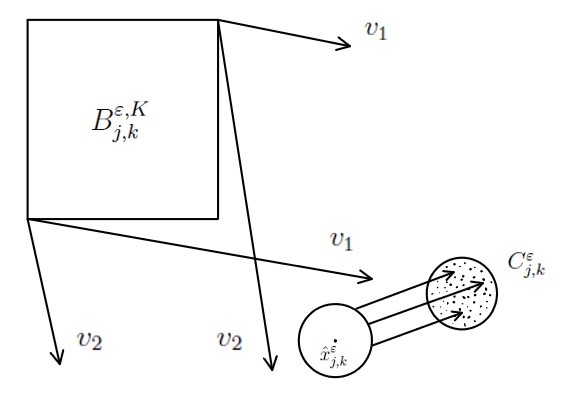
Let the process starting on evolve for a certain period of time. Then, by a local limit theorem, we can estimate from below the probabilities of hitting -sized boxes in a certain -sized region, uniformly in the starting point on .
-
3.
By the parabolic Hörmander condition (H5), we prove a common lower bound for the density of the distribution of the process starting from each of the -sized boxes after a short time.
Let us take care of these steps in order.
Step 1. Let , which will be specified later. We prove in the next two results that the process has a uniformly positive probability of following along the averaged process and going through a neighborhood of the saddle point without making a deviation more than in terms of the value of .
Lemma 5.2.
For each fixed , ,
is uniformly positive for all and sufficiently small.
Proof.
Let the eigenvalues of be bounded by . Recall formula (3.10). By the boundedness of the coefficients, the event
has positive probability, uniformly in the starting points. By (3.10), we have that on the event , for and sufficiently small,
Then Grönwall’s inequality implies that for all . Therefore, implies , and the uniform positivity follows. ∎
Lemma 5.3.
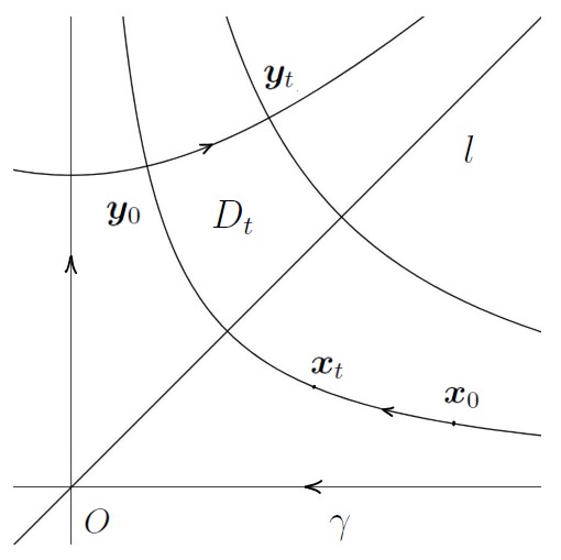
For any given , there exist curves and in such that
-
(i)
and have their tangent vectors as . They intersect with the separatrix on different sides of the saddle point and the averaged motion on the separatrix spends finite time from to .
-
(ii)
Let satisfy and . Then for all , for all sufficiently small.
Proof.
Suppose for all . By the Morse lemma, there exist neighborhoods and of the saddle point and the origin, respectively, and a diffeomorphism from to such that , where . Then consider a random change of time by dividing the generator by :
| (5.2) | ||||
Write the equation for :
It is not hard to verify that satisfies
Hence, by Lemma 3.2, there exists a bounded solution to
Consider a local coordinate and in . The averaged motion has constant speed: in and in . As in (4.1) and (4.2), we have the equations for , , by applying Ito’s formula to and , with , , and :
| (5.3) | ||||
| (5.4) |
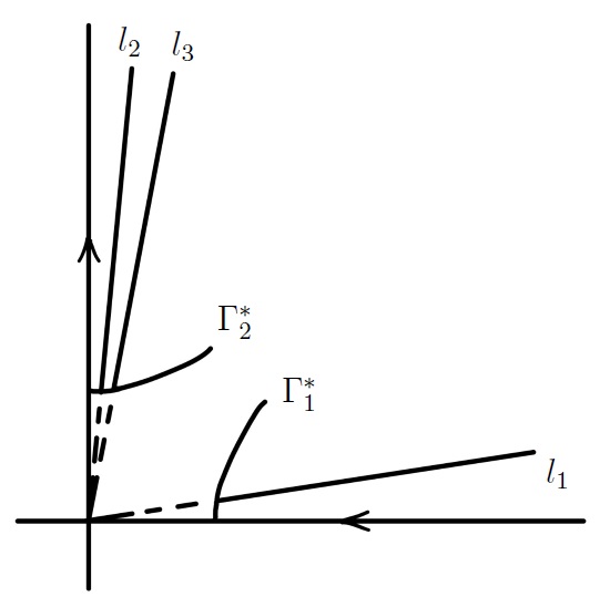
To get the lower bound for the desired probability, we will choose the curves and that are close enough to the saddle point. The time it takes to get from to is still of order since they are chosen independently of . In this way, the process starting on and stopped on will be shown to have small variance, hence it is unlikely for the process to have deviations larger than what we wish. With to be specified later, let , , and . The idea is to look at event that the process stays close to the averaged motion before the latter reaches , which implies that the process does not make a large deviation in , or equivalently, in , before reaching . Let , be the curves that have tangent vectors as and go through the points , , respectively. Since is a diffeomorphism, it is easy to see that each on or with satisfies that . Let and be the pre-images of and in , as shown in Figure 5. They have as tangent vectors due to the specific way we construct and . Consider the process in (5.2) starting at satisfying that with an arbitrary . Let . Define and . Then it is clear that . Let and denote the stochastic integrals in (5.3) and (5.4), respectively, with replaced by . Since , is bounded, and before , we see that the unwanted deviations happen only if and are large. Namely,
Both terms on the right-hand side can be controlled by Chebyshev’s inequality. Note that there exists a constant independent of such that
and, similarly,
Then, can be chosen large enough such that both variances are small enough, and hence . ∎
We can choose the corresponding curves in the other regions. As a result, we have four curves corresponding to four different directions, all with positive distance to the saddle point, as shown in Figure 6. Moreover, the corresponding transition probabilities near the saddle point have lower bounds analogous to that given in Lemma 5.3 (ii). For the rotations happening away from those curves, we will prove that, before the time when the process comes back to the curves, the deviation of can be large enough to cross the separatrix with positive probability. Let be the set .
Lemma 5.4.
For each fixed ,
is positive uniformly in , , and all sufficiently small.
Proof.
By Lemma 5.2 and the Markov property, it is enough to consider small such that does not reach before . Using formula (3.10) again, we see that as uniformly in . Use formula (4.1) on a shorter time scale:
So, it suffices to show the uniform positivity of
Note that there exists another Brownian motion such that
| (5.5) |
Recall that in Subsection 4.1 we defined . Then, by Corollary 3.4,
| (5.6) |
Note that on the event , is uniformly positive for . Let us denote this lower bound as , which is independent of , , and . Then
| (5.7) |
By the convergence in (5.6), we obtain
| (5.8) |
Suppose . Then, for all sufficiently small,
Remark 5.5.
The result in Lemma 5.4 also holds for . Similarly, for each fixed ,
is positive uniformly in , , and sufficiently small.
Now we can choose . By the results in Lemma 5.2, Lemma 5.3, Lemma 5.4, and Remark 5.5, using the strong Markov property, we obtain the following lemma:
Lemma 5.6.
There exists a closed interval on that does not contain the saddle point and a constant satisfying the following property: if the system (3.3) starts at , then for all sufficiently small
| (5.9) |
where .
Remark 5.7.
Step 2. Without loss of generality, we assume that, if starts at one endpoint of , then the other endpoint is . In the remainder of this section, always denotes this deterministic motion, irrespective of where starts. We aim to study the distribution of the process starting on with certain . The choice of will depend on the initial point being considered (see Figure 7), and this will be convenient as we use the strong Markov property later when combining all three steps.
To be more precise, for , let be such that (so ). We introduce a process , , as the second term in the expansion of around the deterministic motion :
| (5.10) |
(Note that, for finite , is of order .) Then, by standard perturbation arguments and Grönwall’s inequality, it can be shown that, uniformly in such that , , and ,
| (5.11) |
Therefore, understanding of the distribution of would help one to understand the distribution of . However, it is not straightforward to study since is not a Markov process. We introduce a related process defined using the original Markov process , apply the local limit theorem to , and use the Girsanov theorem to get the desired estimate. Namely, let , , be defined by:
| (5.12) |
The following result is a version of the local limit theorem [16] adapted to our case.
Theorem 5.8.
Let be a function such that spans and for all , where is the invariant measure of . Then a local limit theorem holds for the following random variable as uniformly in ,
Namely, there exists an invertible covariance matrix continuous in such that
| (5.13) |
uniformly in , , and .
The second term in (5.13) is non-trivial even when takes large values (of order ), which is exactly the situation we are dealing with. Following (5.12), we solve explicitly
| (5.14) |
where solves the differential equation
and is the identity matrix. Since is deterministic, the integrand can be treated as a function only of time and . Moreover, for each , the integrand has zero mean w.r.t. the invariant measure and spans , since is deterministic and non-singular and, for each , spans by assumption (H4′). Then Theorem 5.8 implies that
| (5.15) |
for all small enough, , , and . Finally, we compare with . Since the added drift in the equation of is small compared to the diffusion term , it is not hard to verify that, using the Girsanov theorem, for all small enough, , , and ,
| (5.16) |
Step 3. We proved that reaches the -sized boxes with probabilities bounded from below. We also know that is -close to in . Let us take one generic pair , let , and study the distribution of with the initial point in after time of order (see Figure 8).
Lemma 5.9.
For each , , and , there exist , , and, for each pair , a point such that, for each and all sufficiently small,
where .
Proof.
Recall the definition of at the beginning of Step 2 (see Figure 7). By assumption (H4′), spans . So there exist such that and span . Let us consider the set . Then it is easy to see that, there exist a constant and, for each pair , a point such that for all , and . There exists such that for each and each in , , . Let be the upper bound of vector . For all sufficiently small, the probability of the following event, denoted by , has a lower bound, denoted by , that only depends on , , , , , , , and not on the starting point , thus not on :
where , , and . If is a subset of the event , then the lemma is proved. To show the inclusion, note that on ,
Besides, by the definition of , . Thus on . ∎
From now on, let be the point in assumption (H5) such that the parabolic Hörmander condition holds at and let be the density of starting at .
Lemma 5.10.
There exists such that for each and all sufficiently small, there is a domain with and on for .
Proof.
Consider the stochastic processes that depend on the parameters :
| (5.17) | ||||
Since, by assumption (H5), the parabolic Hörmander condition for equation (1.1) holds at , it is not hard to see that, if is close to and is small, the parabolic Hörmander condition holds for (5.17) at and the distribution of is absolutely continuous w.r.t. the Lebesgue measure ([17]). Moreover, if the density function, denoted by , exists, it is continuous in , and . Let and satisfy that . Then there exists such that exists and is greater than for all , , , , and . For , define . Then, for , and , and , we have that
The result holds with . ∎
Lemma 5.11.
For each , there exist constants and such that for all , there exists a measure and a stopping time such that for each , the distribution of starting at has as a component and for all sufficiently small.
Proof.
Now let us combine Step 2 and Step 3 together to get the following result concerning the total variation distance of with different starting points on :
Lemma 5.12.
For each , let be the measure induced by starting at . Then there exists such that for any and all sufficiently small.
Proof.
It suffices to show that there exist and a stopping time such that the total variation distance of with different starting points on is no more than . Recall the definitions of and in Step 2. For the process starting at , define
Using (5.15) and (5.16), we can find a constant such that, for all , , sufficiently small, and , . And using (3.10) and (5.11) we can choose large enough such that, for all , , and sufficiently small, . Let . Then it is not hard to see that
Now let us define, for ,
Then we know that since, for every ,
Let the constants , , the stopping time , and be defined as in Lemma 5.11. Define
In order to define the desired stopping time, we first run the process starting on for time (with overwhelming probability, it is the time for the deterministic motion with the same stating point to reach ). Then we use the locations of both and to determine whether the process continues and, if it continues, we choose the stopping time based on Lemma 5.11. Namely, we define
| (5.18) |
where denotes the stopping time with initial condition . Then it follows from previous results that, for any pair , there is a common component of the distributions of starting from and , respectively. Moreover, since and . Therefore, the total variation is no more than . ∎
Finally, we combine the result we just obtained with Step 1 to prove Lemma 5.1.
Proof of Lemma 5.1.
As we discussed, the result is equivalent to the exponential convergence in total variation of on , uniformly in and in the initial distribution. Let denote the measure on induced by with the starting point . Then it suffices to prove that there exists such that, for every pair , and all sufficiently small, , which follows from Lemma 5.6 and Lemma 5.12. ∎
6 Proof of the main result
Since we deal with both the original and the auxiliary processes in this section, certain notation needs clarifying to avoid possible ambiguity: the process represents not a generic process with arbitrary bounded but only the auxiliary process with satisfying (3.5); , are defined as in (1.6), but for the process on , and , represent the corresponding stopping time w.r.t. . In (4.4), we defined on each edge for a generic . Here we give a more explicit definition of on the edge :
One can easily check that this is consistent with the definitions of and in (4.4), which are the generalizations of the coefficients defined in (2.2) and, moreover,
| (6.1) |
Lemma 6.1.
For each and all sufficiently small, we have .
Proof.
Let us verify the analogue of (3.2) in the case of the auxiliary process .
Proposition 6.2.
For each and ,
| (6.2) |
as , uniformly in , , and is a stopping time bounded by .
Proof.
We divide the time interval into visits to the separatrix. Since ,
| (6.3) | |||
| (6.4) |
Note that (6.3) converges to due to Proposition 4.6, and (6.4) also converges to since
where the second inequality is due to Lemma 6.1 and the last equality follows from Proposition 4.6, Lemma 5.1, and Proposition B.3. Thus, the desired result holds. ∎
To generalize the result to the original process on , we need the next two technical results. We start with a simple corollary of Lemma 4.16, which controls the number of excursions or, equivalently, the number of stopping times and in finite time.
Corollary 6.3.
For a given , the expected number of excursions before is :
| (6.5) |
where is the constant chosen in Lemma 4.16.
Proof.
Lemma 6.4.
For each and there is such that, for all , , and all sufficiently small,
| (6.8) | ||||
where is a stopping time w.r.t. .
Proof.
The result holds either with or without the integral term since nearly all of the time is spent from to . To be precise, by the strong Markov property, Corollary 6.3, and Proposition B.3,
| (6.9) | ||||
Thus, it suffices to prove for all sufficiently small
| (6.10) |
Let us prove this for first using Proposition 6.2, then apply the Girsanov theorem to get the result for . Let be the analogue of w.r.t. . Divide the time interval into excursions using stopping times and :
| (6.11) | |||
| (6.12) | |||
| (6.13) | |||
| (6.14) |
Thus, (6.13) converges to uniformly for all and due to the convergence of (6.11), (6.12), and (6.14), by Proposition 6.2, Proposition 4.6, and Lemma 4.15 with Corollary 6.3, respectively. Note that (6.9) also holds for , hence we conclude that
| (6.15) |
To apply the Girsanov theorem, we choose a sufficiently small time interval and use the fact that the transition probability of is similar to that of in the sense that they are absolutely continuous with density close to . More precisely, for any fixed , by the Girsanov theorem, we can choose a constant such that for all ,
| (6.16) |
where and are the measures on induced by and . Define
Note that the quantity in (6.10) primarily depends on the behavior of the processes on time interval and event . Indeed, we can replace the stopping times by with errors. To replace with , we need several additional results that control the difference.
As in Corollary 6.3, we fix and choose a large constant independent of such that
| (6.17) |
Now we choose such that, for all , . Hence, for all ,
| (6.18) |
Thus, with , we obtain
| (6.19) |
By following the same steps, we can choose such that for all ,
| (6.20) |
It remains to consider
| (6.21) |
which can be written and estimated as, with denoting the functional on found inside the expectation in (6.21),
| (6.22) | ||||
The first term is bounded by due to (6.15) and (6.20). The second term is simply bounded by . Thus, we see that the left-hand side in (6.10) is no more than with finite independent of and for all sufficiently small. It remains to take . ∎
Proof of Proposition 3.1.
Fix arbitrary . We divide the time interval into excursions from to and from to by using stopping times and :
| (6.23) | |||
| (6.24) | |||
| (6.25) |
Here (6.23) converges to by Proposition 4.6 and (6.25) converges to by Lemma 4.15 and Corollary 6.3. It remains to consider (6.24) and it suffices to consider instead
| (6.26) |
because the difference converges to by Proposition B.3. By Proposition 6.2, we choose such that (6.8) holds for and all sufficiently small. We introduce the stopping times by letting and be the first of such that . It is clear that . Hence, we can replace (6.26) by
| (6.27) |
and, by the strong Markov property, the difference is no more than
| (6.28) |
where is a stopping time w.r.t. . Both of them can be bounded by due to Lemma 6.4 and Corollary 6.3. ∎
Appendix A Derivatives of the action-angle-type coordinates
In this section, we carefully estimate the first and second derivatives of , , , , and in order to prove (4.15). Our main tool is the Morse lemma. Note that we only need to verify the bounds near the separatrix, since the derivatives are uniformly bounded inside the domain. For , let denote the line segment connecting and . For for certain , let denote the piece of connecting to along the direction of . Recall that . To start with, using the Morse lemma, one can compute that and . Then we make use of two special deterministic motions in the directions of and to calculate the first derivatives of precisely:
| (A.1) | ||||
It follows that
| (A.2) |
| (A.3) |
where is the region bounded by , trajectory of , , , and , as shown in Figure 9. Thus, by differentiating (A.2) and (A.3) in , we have the following equations:
| (A.4) | ||||
Therefore, with subscripts denoting the partial derivatives, by solving the linear system,
| (A.5) | ||||
where . Using the Morse lemma, one can compute , since
| (A.6) |
Note that the non-degeneracy of the saddle point implies that , and hence . The next step is to estimate . For all close enough, with denoting the region bounded by , , , and , we have
Then one can obtain by using the Morse lemma again and, as a result, , . Similarly, we can estimate the derivatives of . In fact, because of the estimate we had on . In addition,
| (A.7) |
Since , and , . Finally, we estimate the derivatives w.r.t. of a general function with having bounded first and second derivatives. By computing the inverse of the Jacobian of and using the first equation in (A.4),
| (A.8) |
We deduce that and, using instead of in (A.8), . Similarly, one can obtain and .
Appendix B Exit from neighborhoods of critical points
In this section, we obtain estimates for the exit time from the neighborhoods of the critical points, including extremum points and saddle points. Recall the notation in Section 4: is a saddle point, is an extremum point, is a domain bounded by the separatrix, and . Recall the function defined in (3.8) and let us define
| (B.1) |
Using assumption (H4′), one can see that is positive-definite. Indeed, if there exist a point and a vector such that , then, since is positive-definite, for all . Namely, is constant, and on , which contradicts with (H4′).
Lemma B.1.
Recall the definition of in (4.3). If is a minimum point, then ; if is a maximum point, then .
Proof.
We prove the result in the case of minimum point. The other case can be treated similarly. Since is a critical point and , we have and
This is positive since both and are positive definite at . ∎
Lemma B.2.
For each , there exists such that
| (B.2) |
for all satisfying , , and sufficiently small.
Proof.
Without loss of generality, we assume to be a minimum point. Similarly to (4.1), we apply Ito’s formula to and we obtain
By taking the expectation on both sides and using Corollary 3.4, we obtain
| (B.3) |
Due to Lemma B.1, . Hence, we can choose to be small enough such that before . Thus, it follows from (B.3) that, for all sufficiently small,
Then for all satisfying , by Markov’s inequality. Then, one can obtain the desired result using the Markov property by the fact that . ∎
Proposition B.3.
Let , , and . Then, uniformly in and , as ,
| (B.4) |
To prove Proposition B.3, it is more convenient to consider the process , define the stopping time , and then prove that . We need careful analysis of the behavior of the processes near the saddle point and away from the saddle point. The latter is easier to deal with since there is no degeneracy, while the former needs us to, again, use the Morse Lemma to make concrete computations. For simplicity, we prove the result in the case of without the additional drift since it can be seen in the proof that the additional terms induced by are always relatively small. We prove that there exist two neighborhoods, , of (as shown in Figure 10(a)), such that, in , it takes the process time to escape from , and time to return to . Since is two-dimensional, we denote . To avoid confusion brought by convoluted formulas, we assume the saddle point is the origin and the Hamiltonian in a small neighborhood of . This assumption is not restrictive because, as in the proof of Lemma 5.3, we can use the Morse Lemma and perform a random change of time with the multiplier bounded from below and above, which will not change the order of the expected time. For , we denote to be the region in with and , , , and choose small enough that in .
Lemma B.4.
There exist such that, uniformly in , as ,
| (B.5) |
where .
Proof.
We denote and study the behavior of inside . All the computations below concern before leaving . As in (3.10), we can write the equation for ,
| (B.6) | ||||
Introduce , which is close to :
| (B.7) |
Let , which satisfies , as , and has bounded derivatives up to the third order. Then we can choose a large , such that , are bounded by . Recall from (B.1) that the vector-valued function has non-degenerate average w.r.t. , in the sense that . Let and let be such that in , as shown in Figure 10(b). Let . Define function (that depends on ) and compute its derivatives:
| (B.8) | ||||
Furthermore, satisfies the differential equations:
| (B.9) |
By Lemma 3.2, there is a function that is bounded together with its derivatives such that
| (B.10) |
where is the generator of the process (see (2.1)). Since and , we can apply Ito’s formula to for :
| (B.11) | ||||
Hence it follows that
| (B.12) | ||||
Now apply Ito’s formula to for :
where the equalities follow from (B.8) and (B.12), and the last inequality holds since solves (B.9) and . Let . Then because . The previous calculation reduces to
By taking the expectation, we have for all , , and small enough
| (B.13) |
Then, by Markov’s inequality and the Markov property, we obtain that . ∎
Lemma B.5.
Let be defined as in Lemma B.4. Then, uniformly in ,
| (B.14) |
Proof.
Again, we denote and, for simplicity, we assume that the saddle point is the origin and that in a small neighborhood of . We extend the function in the vertical direction in such a way that it is bounded together with its partial derivatives and the first component of is in the region . We denote and show that it takes significantly longer than for to reach , hence it is unlikely for to exit through . All the computations below concern before reaches . As in (3.10), we can write the equation for :
| (B.15) | ||||
Introduce , which is close to :
| (B.16) |
Since and its partial derivatives are bounded in , we can choose such that
| (B.17) |
Let us define , , and function . Then it follows that
| (B.18) |
Note that for since . Apply Ito’s formula to for and obtain using (B.17):
The last inequality follows from (B.18) and the fact that the integrand on the second line is either negative, when , or small and bounded by , when . By replacing by the stopping time and taking expectation, we obtain
| (B.19) |
Let . Then, since , it follows that
| (B.20) |
as . However, by Lemma B.4 and Markov’s inequality, we have
| (B.21) |
as . Thus, the desired result follows. ∎
Lemma B.6.
Let . Then there exists such that, uniformly in ,
| (B.22) |
Furthermore, is bounded uniformly in .
Proof.
Let and be the lower bound and the upper bound of time spent by to get from to , respectively. Then, similarly to (5.8), there exists such that
| (B.23) |
Hence
Similarly, it is easy to see that , and the desired result follows from the Markov property. ∎
Proof of Proposition B.3.
As in (4.1):
The change in is mainly due to the stochastic integral while the other terms are of order and and can be controlled. For each ,
| (B.24) | ||||
Note that if we choose , then the second event is always true. Now we recursively define stopping times:
We denote . Note that once the process leaves , the stopping times stay constant afterwards. The main idea of the proof is to show that after a sufficiently long time , the stochastic integral will accumulate enough variance to exit from . Let us bound the probability of variance being small:
| (B.25) | ||||
where the integer will be specified later. Let , , and be defined as in Lemma B.4 and Lemma B.6. Then
| (B.26) | |||
Now let us deal with one excursion from to . For ,
| (B.27) | ||||
for all sufficiently small, by Lemma B.6. For :
by Lemma B.5 and (B.27). Now we can come back to (B.26) and have
| (B.28) |
The second probability on the right-hand side of (B.25) can be bounded by Lemmas B.4 and B.6 with certain :
| (B.29) | ||||
Choose . Then the quantity in (B.28) converges to . Choose , then the quantity on the right-hand side of (B.29) converges to . Therefore, the quantity on the right-hand side of (B.25) converges to . Moreover, since , it follows from (B.24) that, for all , , and sufficiently small,
since the stochastic integral in the last inequality can be represented as time-changed Brownian motion. Finally, we have by the Markov property
Appendix C Tightness
In this section, we verify the tightness for the projection to the Reeb graph of the original process (1.4) on . By the Arzelà–Ascoli theorem (cf. Theorem 7.3 in [1]), it suffices to check the following two conditions
| (C.1) | |||
| (C.2) |
hold for all and . As in (4.1), we can also write the equation for , where we consider to be a process on :
| (C.3) | ||||
By assumption (H4) and Lemma 3.2, is bounded together with its first derivatives. Besides, by assumption (H2), as , hence as . Also, there exists an such that and for all . For , let . Then, by Markov’s inequality and boundedness of second derivatives of ,
as , uniformly in . Thus, we have (C.1), and it also follows that
| (C.4) |
since and has bounded second derivatives. To verify (C.2), we see that, for an arbitrary small,
Since (C.4) holds, it is sufficient to prove, for each ,
| (C.5) |
Let be the upper bound for , , , and eigenvalues of and over . On the event the following holds. For , due to (C.3) and the fact that the stochastic integral can be represented as a time-changed Brownian motion, we have
where is another Brownian motion. Hence, for sufficiently small, independently of ,
as , since each term is exponentially small as . This proves (C.5), and thus (C.2).
Acknowledgements
I am grateful to Mark Freidlin for introducing me to this problem and to my advisor Leonid Koralov for invaluable guidance. I am also grateful to Dmitry Dolgopyat and Yeor Hafouta for insightful discussions.
References
- [1] Patrick Billingsley “Convergence of probability measures” A Wiley-Interscience Publication, Wiley Series in Probability and Statistics: Probability and Statistics John Wiley & Sons, Inc., New York, 1999, pp. x+277
- [2] A.. Borodin “A limit theorem for the solutions of differential equations with a random right-hand side” In Teor. Verojatnost. i Primenen. 22.3, 1977, pp. 498–512
- [3] A.. Borodin and M.. Freidlin “Fast oscillating random perturbations of dynamical systems with conservation laws” In Ann. Inst. H. Poincaré Probab. Statist. 31.3, 1995, pp. 485–525
- [4] Dmitry Dolgopyat, Mark Freidlin and Leonid Koralov “Deterministic and stochastic perturbations of area preserving flows on a two-dimensional torus” In Ergodic Theory Dynam. Systems 32.3, 2012, pp. 899–918
- [5] Dmitry Dolgopyat and Leonid Koralov “Averaging of Hamiltonian flows with an ergodic component” In Ann. Probab. 36.6, 2008, pp. 1999–2049
- [6] Dmitry Dolgopyat and Leonid Koralov “Averaging of incompressible flows on two-dimensional surfaces” In J. Amer. Math. Soc. 26.2, 2013, pp. 427–449
- [7] Stewart N. Ethier and Thomas G. Kurtz “Markov processes” Characterization and convergence, Wiley Series in Probability and Mathematical Statistics: Probability and Mathematical Statistics John Wiley & Sons, Inc., New York, 1986, pp. x+534
- [8] M. Freidlin and L. Koralov “Averaging in the case of multiple invariant measures for the fast system” In Electron. J. Probab. 26, 2021, pp. Paper No. 138\bibrangessep17
- [9] M.. Freidlin and A.. Wentzell “Diffusion approximation for noise-induced evolution of first integrals in multifrequency systems” In J. Stat. Phys. 182.3, 2021, pp. Paper No. 45\bibrangessep24
- [10] Mark Freidlin and Matthias Weber “Random perturbations of dynamical systems and diffusion processes with conservation laws” In Probab. Theory Related Fields 128.3, 2004, pp. 441–466
- [11] Mark I. Freidlin and Alexander D. Wentzell “Random perturbations of dynamical systems” Translated from the 1979 Russian original by Joseph Szücs 260, Grundlehren der mathematischen Wissenschaften [Fundamental Principles of Mathematical Sciences] Springer, Heidelberg, 2012, pp. xxviii+458
- [12] Mark I. Freidlin and Alexander D. Wentzell “Random perturbations of Hamiltonian systems” In Mem. Amer. Math. Soc. 109.523, 1994, pp. viii+82
- [13] Martin Hairer “On Malliavin’s proof of Hörmander’s theorem” In Bull. Sci. Math. 135.6-7, 2011, pp. 650–666
- [14] R.. Has’minskii “A limit theorem for solutions of differential equations with a random right hand part” In Teor. Verojatnost. i Primenen. 11, 1966, pp. 444–462
- [15] R.. Has’minskii “Ergodic properties of recurrent diffusion processes and stabilization of the solution of the Cauchy problem for parabolic equations” In Teor. Verojatnost. i Primenen. 5, 1960, pp. 196–214
- [16] Leonid Koralov and Shuo Yan “Local limit theorem for time-inhomogeneous functions of Markov processes”, 2024 arXiv:2308.00880 [math.PR]
- [17] David Nualart “The Malliavin calculus and related topics”, Probability and its Applications (New York) Springer-Verlag, Berlin, 2006, pp. xiv+382