Fast and Secure Distributed
Nonnegative Matrix Factorization
Abstract
Nonnegative matrix factorization (NMF) has been successfully applied in several data mining tasks. Recently, there is an increasing interest in the acceleration of NMF, due to its high cost on large matrices. On the other hand, the privacy issue of NMF over federated data is worthy of attention, since NMF is prevalently applied in image and text analysis which may involve leveraging privacy data (e.g, medical image and record) across several parties (e.g., hospitals). In this paper, we study the acceleration and security problems of distributed NMF. Firstly, we propose a distributed sketched alternating nonnegative least squares (DSANLS) framework for NMF, which utilizes a matrix sketching technique to reduce the size of nonnegative least squares subproblems with a convergence guarantee. For the second problem, we show that DSANLS with modification can be adapted to the security setting, but only for one or limited iterations. Consequently, we propose four efficient distributed NMF methods in both synchronous and asynchronous settings with a security guarantee. We conduct extensive experiments on several real datasets to show the superiority of our proposed methods. The implementation of our methods is available at https://github.com/qianyuqiu79/DSANLS.
Index Terms:
Distributed Nonnegative Matrix Factorization, Matrix Sketching, Privacy1 Introduction
Nonnegative matrix factorization (NMF) is a technique for discovering nonnegative latent factors and/or performing dimensionality reduction. Unlike general matrix factorization (MF), NMF restricts the two output matrix factors to be nonnegative. Specifically, the goal of NMF is to decompose a huge matrix into the product of two matrices and such that . denotes the set of matrices with nonnegative real values, and is a user-specified dimensionality, where typically . Nonnegativity is inherent in the feature space of many real-world applications, where the resulting factors of NMF can have a natural interpretation. Therefore, NMF has been widely used in a branch of fields including text mining [1], image/video processing [2], recommendation [3], and analysis of social networks [4].
Modern data analysis tasks apply on big matrix data with increasing scale and dimensionality. Examples [5] include community detection in a billion-node social network, background separation on a 4K video in which every frame has approximately 27 million rows, and text mining on a bag-of-words matrix with millions of words. The volume of data is anticipated to increase in the ‘big data’ era, making it impossible to store the whole matrix in the main memory throughout NMF. Therefore, there is a need for high-performance and scalable distributed NMF algorithms. On the other hand, there is a surge of works on privacy-preserving data mining over federated data [6, 7] in recent years. In contrast to traditional research about privacy which emphasizes protecting individual information from single institution, federated data mining deals with multiple parties. Each party possesses its own confidential dataset(s) and the union of data from all parties is utilized for achieving better performance in the target task. Due to the prevalent use of NMF in image and text analysis which may involve leveraging privacy data (e.g, medical image and record) across several parties (e.g., hospitals), the privacy issue of NMF over federated data is worthy of attention. To address aforementioned challenges of NMF (i.e., high performance and privacy), we study the acceleration and security problems of distributed NMF in this paper.
First of all, we propose the distributed sketched alternating nonnegative least squares (DSANLS) for accelerating NMF. The state-of-the-art distributed NMF is MPI-FAUN [8], a general framework that iteratively solves the nonnegative least squares (NLS) subproblems for and . The main idea behind MPI-FAUN is to exploit the independence of local updates for rows of and , in order to minimize the communication requirements of matrix multiplication operations within the NMF algorithms. Unlike MPI-FAUN, our idea is to speed up distributed NMF in a new, orthogonal direction: by reducing the problem size of each NLS subproblem within NMF, which in turn decreases the overall computation cost. In a nutshell, we reduce the size of each NLS subproblem, by employing a matrix sketching technique: the involved matrices in the subproblem are multiplied by a specially designed random matrix at each iteration, which greatly reduces their dimensionality. As a result, the computational cost of each subproblem significantly drops.
However, applying matrix sketching comes with several issues. First, although the size of each subproblem is significantly reduced, sketching involves matrix multiplication which brings computational overhead. Second, unlike in a single machine setting, data is distributed to different nodes in distributed environment. Nodes may have to communicate extensively in a poorly designed solution. In particular, each node only retains part of both the input matrix and the generated approximate matrices, causing difficulties due to data dependencies in the computation process. Besides, the generated random matrices should be the same for all nodes in every iteration, while broadcasting the random matrix to all nodes brings severe communication overhead and can become the bottleneck of distributed NMF. Furthermore, after reducing each original subproblem to a sketched random new subproblem, it is not clear whether the algorithm still converges and whether it converges to stationary points of the original NMF problem.
Our DSANLS overcomes these problems. Firstly, the extra computation cost due to sketching is reduced with a proper choice of the random matrices. Then, the same random matrices used for sketching are generated independently at each node, thus there is no need for transferring them among nodes during distributed NMF. Having the complete random matrix at each node, an NMF iteration can be done locally with the help of a matrix multiplication rule with proper data partitioning. Therefore, our matrix sketching approach reduces not only the computational overhead, but also the communication cost. Moreover, due to the fact that sketching also shifts the optimal solution of each original NMF subproblem, we propose subproblem solvers paired with theoretical guarantees of their convergence to a stationary point of the original subproblems.
To provide solutions to the problem of secure distributed NMF over federated data, we first show that DSANLS with modification can be adapted to this security setting, but only for one or limited iterations. Therefore, we design new methods called Syn-SD and Syn-SSD in synchronous setting. They are later extended to Asyn-SD and Asyn-SSD in asynchronous setting (i.e., client/server), respectively. Syn-SSD improves the convergence rate of Syn-SD, without incurring much extra communication cost. It also reduces computational overhead by sketching. All proposed algorithms are secure with a guarantee. Secure distributed NMF problem is hard in nature. All parties involved should not be able to infer the confidential information during the process. To the best of our knowledge, we are the first to study NMF over federated data.
In summary, our contributions are as follows:
-
•
DSANLS is the first distributed NMF algorithm that leverages matrix sketching to reduce the problem size of each NLS subproblem and can be applied to both dense and sparse input matrices with a convergence guarantee.
-
•
We propose a novel and specially designed subproblem solver (proximal coordinate descent), which helps DSANLS converge faster. We also discuss the use of projected gradient descent as subproblem solver, showing that it is equivalent to stochastic gradient descent (SGD) on the original (non-sketched) NLS subproblem.
-
•
For the problem of secure distributed NMF, we propose efficient methods, Syn-SD and Syn-SSD, in synchronous setting and later extend them to asynchronous setting. Through sketching, their computation cost is significantly reduced. They are the first secure distributed NMF methods for federated data.
-
•
We conduct extensive experiments using several (dense and sparse) real datasets, which demonstrates the efficiency and scalability of our proposals.
The remainder of the paper is organized as follows. Sec. 2 provides the background and discusses the related work. Our DSANLS algorithm with detailed theoretical analysis is presented in Sec. 3. Our proposed algorithms for secure distributed NMF problem in both synchronous and asynchronous settings are presented in Sec. 4. Sec. 5 evaluates all algorithms. Finally, Sec. 6 concludes the paper.
Notations. For a matrix , we use to denote the entry at the -th row and -th column of . Besides, either or can be omitted to denote a column or a row, i.e., is the -th row of , and is its -th column. Furthermore, or can be replaced by a subset of indices. For example, if , denotes the sub-matrix of formed by all rows in , whereas is the sub-matrix of formed by all columns in a subset .
2 Background and Related Work
In Sec. 2.1, we first illustrate NMF and its security problem in a distributed environment. Then we elaborate on previous works which are related to this paper in Sec. 2.2.
2.1 Preliminary
2.1.1 NMF Algorithms
Generally, NMF can be defined as an optimization problem [9] as follows:
| (1) |
where is the Frobenius norm of . Problem (1) is hard to solve directly because it is non-convex. Therefore, almost all NMF algorithms leverage two-block coordinate descent schemes (shown in Alg. 1): they optimize over one of the two factors, or , while keeping the other fixed [10]. By fixing , we can optimize by solving a nonnegative least squares (NLS) subproblem:
| (2) |
Similarly, if we fix , the problem becomes:
| (3) |
Input:
Parameter: Iteration number
Within two-block coordinate descent schemes (exact or inexact), different subproblem solvers are proposed. The first widely used update rule is Multiplicative Updates (MU) [11, 9]. MU is based on the majorization-minimization framework and its application guarantees that the objective function monotonically decreases [11, 9]. Another extensively studied method is alternating nonnegative least squares (ANLS), which represents a class of methods where the subproblems for and are solved exactly following the framework described in Alg. 1. ANLS is guaranteed to converge to a stationary point [12] and has been shown to perform very well in practice with active set [13, 14], projected gradient [15], quasi-Newton [16], or accelerated gradient [17] methods as the subproblem solver. Therefore, we focus on ANLS in this paper.
2.1.2 Secure Distributed NMF
Secure distributed NMF problem is meaningful with practical applications. Suppose two hospitals and have different clinical records, and (i.e., matrices), for same set of phenotypes. For legal or commercial concerns, it is required that none of the hospitals can reveal personal records to another directly. For the purpose of phenotype classification, NMF task can be applied independently (i.e., and ). However, since and have the same schema for phenotypes, the concatenated matrix can be taken as input for NMF and results in better user (i.e., patients) latent representations and by sharing the same item (i.e., phenotypes) latent representation :
| (4) |
Throughout the factorization process, a secure distributed NMF should guarantee that party only has access to , and and party only has access to , and . It is worth noting that the above problem of distributed NMF with two parties can be straightforwardly extended to parties. The requirement of all parties over federated data in secure distributed NMF is actual the so-called -private protocol (shown in Definition 1 with ) which derives from secure function evaluation [18]. In this paper, we will use it to assess whether a distributed NMF is secure.
Definition 1.
(-private protocol). All parties follow the protocol honestly, but they are also curious about inferring other party’s private information based on their own data (i.e., honest-but-curious). A protocol is -private if any parties who collude at the end of the protocol learn nothing beyond their own outputs.
Note that a single matrix transpose operation transforms a column-concatenated matrix to a row-concatenated matrix. Without loss of generality, we only consider the scenario that matrices are concatenated along rows in this paper.
Secure distributed NMF problem is hard in nature. Firstly, party needs to solve the NMF problem to get and together with party . At the same time, party should not be able to infer or during the whole process. Such secure requirement makes it totally different from traditional distributed NMF problem, whose data partition already incurs secure violation.
2.2 Related Work
In the sequel, we briefly review three research areas which are related to this paper.
2.2.1 Accelerating NMF
Parallel NMF algorithms are well studied in the literature [19, 20]. However, different from a parallel and single machine setting, data sharing and communication have considerable cost in a distributed setting. Therefore, we need specialized NMF algorithms for massive scale data handling in a distributed environment. The first method in this direction [21] is based on the MU algorithm. It mainly focuses on sparse matrices and applies a careful partitioning of the data in order to maximize data locality and parallelism. Later, CloudNMF [22], a MapReduce-based NMF algorithm similar to [21], was implemented and tested on large-scale biological datasets. Another distributed NMF algorithm [23] leverages block-wise updates for local aggregation and parallelism. It also performs frequent updates using whenever possible the most recently updated data, which is more efficient than traditional concurrent counterparts. Apart from MapReduce implementations, Spark is also attracting attention for its advantage in iterative algorithms, e.g., using MLlib [24]. Finally, there are implementations using X10 [25] and on GPU [26].
The most recent and related work in this direction is MPI-FAUN [5, 8], which is the first implementation of NMF using MPI for interprocessor communication. MPI-FAUN is flexible and can be utilized for a broad class of NMF algorithms that iteratively solve NLS subproblems including MU, HALS, and ANLS/BPP. MPI-FAUN exploits the independence of local update computation for rows of and to apply communication-optimal matrix multiplication. In a nutshell, the full matrix is split across a two-dimensional grid of processors and multiple copies of both and are kept at different nodes, in order to reduce the communication between nodes during the iterations of NMF algorithms.
2.2.2 Matrix Sketching
Matrix sketching is a technique that has been previously used in numerical linear algebra [27], statistics [28] and optimization [29]. Its basic idea is described as follows. Suppose we need to find a solution to the equation: . Instead of solving this equation directly, in each iteration of matrix sketching, a random matrix is generated, and we instead solve the following problem: . Obviously, the solution to the first equation is also a solution to the second equation, but not vice versa. However, the problem size has now decreased from to . With a properly generated random matrix and an appropriate method to solve subproblem in the second equation, it can be guaranteed that we will progressively approach the solution to the first equation by iteratively applying this sketching technique.
To the best of our knowledge, there is only one piece of previous work [30] which incorporates dual random projection into the NMF problem, in a centralized environment, sharing similar ideas as SANLS, the centralized version of our DSANLS algorithm. However, Wang et al. [30] did not provide an efficient subproblem solver, and their method was less effective than non-sketched methods in practical experiments. Besides, data sparsity was not taken into consideration in their work. Furthermore, no theoretical guarantee was provided for NMF with dual random projection. In short, SANLS is not same as [30] and DSANLS is much more than a distributed version of [30]. The methods that we propose in this paper are efficient in practice and have strong theoretical guarantees.
2.2.3 Secure Matrix Computation on Federated Data
In federated data mining, parties collaborate to perform data processing task on the union of their unencrypted data, without leaking their private data to other participants [31]. A surge of work in the literature studies federated matrix computation algorithms, such as privacy-preserving gradient descent [32, 33], eigenvector computation [34], singular value decomposition [35, 36], k-means clustering [37], and spectral clustering [38] over partitioned data on different parties. Secure multi-party computation (MPC) are applied to preserve the privacy of the parties involved (e.g. secure addition, secure multiplication and secure dot product) [39, 37]. These Secure MPC protocols compute arbitrary function among parties and tolerate up to corrupted parties, at a cost per bit [40, 41]. These protocols are too generic when it comes to a specific task like secure NMF. Our proposed protocol does not incorporate costly MPC multiplication protocols while tolerates up to -1 corrupted (static, honest but curious) parties. Recently, Kim et al. [6] proposed a federated method to learn phenotypes across multiple hospitals with alternating direction method of multipliers (ADMM) tensor factorization; and Feng et al. [7] developed a privacy-preserving tensor decomposition framework for processing encrypted data in a federated cloud setting.
3 DSANLS: Distributed Sketched ANLS
In this section, we illustrate our DSANLS method for accelerating NMF in general distributed environment.
3.1 Data Partitioning
Assume there are computing nodes in the cluster. We partition the row indices of the input matrix into disjoint sets , where is the subset of rows assigned to node , as in [21]. Similarly, we partition the column indices into disjoint sets and assign column set to node . The number of rows and columns in each node are near the same in order to achieve load balancing, i.e., and for each node . The factor matrices and are also assigned to nodes accordingly, i.e., node stores and updates and as shown in Fig. 1(a).


Data partitioning in distributed NMF differs from that in parallel NMF. Previous works on parallel NMF [19, 20] choose to partition and along the long dimension, but we adopt the row-partitioning of and as in [21]. To see why, take the -subproblem (2) as an example and observe that it is row-independent in nature, i.e., the -th row block of its solution is given by:
| (5) |
and thus can be solved independently without referring to any other row blocks of . The same holds for the -subproblem. In addition, no communication is needed concerning when solving (5) because is already present in node .
On the other hand, solving (5) requires the entire of size , meaning that every node needs to gather from all other nodes. This process can easily be the bottleneck of a naive distributed ANLS implementation. As we will explain shortly, our DSALNS algorithm alleviates this problem, since we use a sketched matrix of reduced size instead of the original complete matrix .
3.2 SANLS: Sketched ANLS
To better understand DSANLS, we first introduce the Sketched ANLS (SANLS), i.e., a centralized version of our algorithm. Recall that in Sec. 2.1.1, at each step of ANLS, either or is fixed and we solve a nonnegative least square problem (2) or (3) over the other variable. Intuitively, it is unnecessary to solve this subproblem with high accuracy, because we may not have reached the optimal solution for the fixed variable so far. Hence, when the fixed variable changes in the next step, this accurate solution from the previous step will not be optimal anymore and will have to be re-computed. Our idea is to apply matrix sketching for each subproblem, in order to obtain an approximate solution for it at a much lower computational and communication cost.
Specifically, suppose we are at the -th iteration of ANLS, and our current estimations for and are and respectively. We must solve subproblem (2) in order to update to a new matrix . We apply matrix sketching to the residual term of subproblem (2). The subproblem now becomes:
| (6) |
where is a randomly-generated matrix. Hence, the problem size decreases from to . is chosen to be much smaller than , in order to sufficiently reduce the computational cost111However, we should not choose an extremely small , otherwise the the size of sketched subproblem would become so small that it can hardly represent the original subproblem, preventing NMF from converging to a good result. In practice, we can set for medium-sized matrices and for large matrices if . When and differ a lot, e.g., without loss of generality, we should not apply sketching technique to the subproblem (since solving the subproblem is much more expensive) and simply choose . . Similarly, we transform the -subproblem into:
| (7) |
where is also a random matrix with .
3.3 DSANLS: Distributed SANLS
Now, we come to our proposal: the distributed version of SANLS called DSANLS. Since the -subproblem (6) is the same as the -subproblem (7) in nature, here we restrict our attention to the -subproblem. The first observation about subproblem (6) is that it is still row-independent, thus node only needs to solve:
| (8) |
For simplicity, we denote:
| (9) |
and the subproblem (8) can be written as:
| (10) |
Thus, node needs to know matrices and in order to solve the subproblem.
For , by applying matrix multiplication rules, we get . Therefore, if is stored at node , can be computed without any communication. On the other hand, computing requires communication across the whole cluster, since the rows of are distributed across different nodes. Fortunately, if we assume that is stored at all nodes again, we can compute in a much cheaper way. Following block matrix multiplication rules, we can rewrite as:
| (11) |
Note that the summand is a matrix of size and can be computed locally. As a result, communication is only needed for summing up the matrices of size by using MPI all-reduce operation, which is much cheaper than transmitting the whole of size .
Now, the only remaining problem is the transmission of . Since can be dense, even larger than , broadcasting it across the whole cluster can be quite expensive. However, it turns out that we can avoid this. Recall that is a randomly-generated matrix; each node can generate exactly the same matrix, if we use the same pseudo-random generator and the same seed. Therefore, we only need to broadcast the random seed, which is just an integer, at the beginning of the whole program. This ensures that each node generates exactly the same random number sequence and hence the same random matrices at each iteration.
In short, the communication cost of each node is reduced from to by adopting our sketching technique for the -subproblem. Likewise, the communication cost of each -subproblem is decreased from to . The general framework of our DSANLS algorithm is listed in Alg. 2.
Input: and
Parameter: Iteration number
3.4 Generation of Random Matrices
A key problem in Alg. 2 is how to generate random matrices and . Here we focus on generating a random satisfying Assumption 1. The reason for choosing such a random matrix is that the corresponding sketched problem would be equivalent to the original problem on expectation; we will prove this in Sec. 3.5.
Assumption 1.
Assume the random matrices are normalized and have bounded variance, i.e., there exists a constant such that for all , where is the identity matrix.
Different options exist for such matrices, which have different computation costs in forming sketched matrices and . Since is much larger than and thus computing is more expensive, we only consider the cost of constructing here.
The most classical choice for a random matrix is one with i.i.d. Gaussian entries having mean 0 and variance . It is easy to show that . Besides, Gaussian random matrix has bounded variance because Gaussian distribution has finite fourth-order moment. However, since each entry of such a matrix is totally random and thus no special structure exists in , matrix multiplication will be expensive. That is, when given of size , computing its sketched matrix requires basic operations.
A seemingly better choice for would be a subsampling random matrix. Each column of such random matrix is uniformly sampled from without replacement, where is the -th canonical basis vector (i.e., a vector having its -th element 1 and all others 0). We can easily show that such an also satisfies and the variance is bounded, but this time constructing the sketched matrix only requires . Besides, subsampling random matrix can preserve the sparsity of original matrix. Hence, a subsampling random matrix would be favored over a Gaussian random matrix by most applications, especially for very large-scale or sparse problems. On the other hand, we observed in our experiments that a Gaussian random matrix can result in a faster per-iteration convergence rate, because each column of the sketched matrix contains entries from multiple columns of the original matrix and thus is more informative. Hence, it would be better to use a Gaussian matrix when the sketch size is small and thus a complexity is acceptable, or when the network speed of the cluster is poor, hence we should trade more local computation cost for less communication cost.
Although we only test two representative types of random matrices (i.e., Gaussian and subsampling random matrices), our framework is readily applicable for other choices, such as subsampled randomized Hadamard transform (SRHT) [42, 43] and count sketch [44, 45]. The choice of random matrices is not the focus of this paper and left for future investigation.
3.5 Solving Subproblems
Before describing how to solve subproblem (10), let us make an important observation. As discussed in Sec. 2.2.2, the sketching technique has been applied in solving linear systems before. However, the situation is different in matrix factorization. Note that for the distributed matrix factorization problem we usually have:
| (12) |
So, for the sketched subproblem (10), which can be equivalently written as:
| (13) |
where the non-zero entries of the residual matrix will be scaled by the matrix at different levels. As a consequence, the optimal solution will be shifted because of sketching. This fact alerts us that for SANLS, we need to update by exploiting the sketched subproblem (10) to step towards the true optimal solution and avoid convergence to the solution of the sketched subproblem.
3.5.1 Projected Gradient Descent
A natural method is to use one step222Note that we only apply one step of projected gradient descent here to avoid solution shifted. of projected gradient descent for the sketched subproblem:
| (14) | ||||
where is the step size and denotes the entry-wise maximum operation. In the gradient descent step (14), the computational cost mainly comes from two matrix multiplications: and . Note that and are of sizes and respectively, thus the gradient descent step takes in total.
To exploit the nature of this algorithm, we further expand the gradient:
| (15) | ||||
By taking the expectation of the above equation, and using the fact , we have:
| (16) | ||||
which means that the gradient of the sketched subproblem is equivalent to the gradient of the original problem on expectation. Therefore, such a step of gradient descent can be interpreted as a (generalized) stochastic gradient descent (SGD) [46] method on the original subproblem. Thus, according to the theory of SGD, we naturally require the step sizes to be diminishing, i.e., as increases.
3.5.2 Proximal Coordinate Descent
However, it is well known that the gradient descent method converges slowly, while the coordinate descent method, namely the HALS method for NMF, is quite efficient [10]. Still, because of its very fast convergence, HALS should not be applied to the sketched subproblem directly because it shifts the solution away from the true optimal solution. Therefore, we would like to develop a method which resembles HALS but will not converge towards the solutions of the sketched subproblems.
To achieve this, we add a regularization term to the sketched subproblem (10). The new subproblem becomes:
| (17) |
where is a parameter. Such regularization is reminiscent to the proximal point method [47] and parameter controls the step size as in projected gradient descent. We therefore require to enforce the convergence of the algorithm, e.g., .
At each step of proximal coordinate descent, only one column of , say where , is updated:
| (18) |
It is not hard to see that the above problem is still row-independent, which means that each entry of the row vector can be solved independently at each node. For example, for any , the solution of is given by:
| (19) | ||||
At each step of coordinate descent, we choose the column from successively. When updating column at iteration , the columns have already been updated and thus , while the columns are old so .
The complete proximal coordinate descent algorithm for the -subproblem is summarized in Alg. 3. When updating column , computing the matrix-vector multiplication takes . The whole inner loop takes because one vector dot product of length is required for computing each summand and the summation itself needs . Considering that there are columns in total, the overall complexity of coordinate descent is . Typically, we choose , so the complexity can be simplified to , which is the same as that of gradient descent.
Since proximal coordinate descent is much more efficient than projected gradient descent, we adopt it as the default subproblem solver within DSANLS.
Parameter:
3.6 Theoretical Analysis
3.6.1 Complexity Analysis
We now analyze the computational and communication costs of our DSANLS algorithm, when using subsampling random sketch matrices. The computational complexity at each node is:
| (20) | ||||
Moreover, as we have shown in Sec. 3.3, the communication cost of DSANLS is .
On the other hand, for a classical implementation of distributed HALS [48], the computational cost is:
| (21) |
and the communication cost is due to the all-gathering of ’s.
Comparing the above quantities, we observe an speedup of our DSANLS algorithm over HALS in both computation and communication. However, we empirically observed that DSANLS has a slower per-iteration convergence rate (i.e., it needs more iterations to converge). Still, as we will show in the next section, in practice, DSANLS is superior to alternative distributed NMF algorithms, after taking all factors into account.
3.6.2 Convergence Analysis
Here we provide theoretical convergence guarantees for the proposed SANLS and DSANLS algorithms. We show that SANLS and DSANLS converge to a stationary point.
To establish convergence result, Assumption 2 is needed first.
Assumption 2.
Assume all the iterates and have uniformly bounded norms, which means that there exists a constant such that and for all .
We experimentally observed that this assumption holds in practice, as long as the step sizes used are not too large. Besides, Assumption 2 can also be enforced by imposing additional constraints, such as:
| (22) |
with which we have . Such constraints can be very easily handled by both of our projected gradient descent and regularized coordinate descent solvers. Lemma 1 shows that imposing such extra constraints does not prevent us from finding the global optimal solution.
Lemma 1.
Based on Assumptions 1 (see Sec. 3.4) and Assumption 2, we now can formally show our main convergence result:
Theorem 1.
4 Secure Distributed NMF
In this section, we provide our solutions to the problem of secure distributed NMF over federated data.
4.1 Extend DSANLS to Secure Setting
DSANLS and all lines of works discussed in Sec. 2.2.1 store copies of across two-dimensional (shown in Fig. 1(a)), and exploit the independence of local update computation for rows of and to apply communication-optimal matrix multiplication. They cannot be applied directly to secure distributed NMF setting. The reason is that, in secure distributed NMF setting (shown in Fig. 1(b)), only one column copy is stored in each node, while the others cannot be disclosed.
Nevertheless, DSANLS can be adapted to this secure setting with modification, but only for one or limited iterations. The reason is illustrated in Theorem 2. In modified DSANLS algorithm, each node still takes charge of updating and as before, but only one copy of will be stored in node . Thus, -subproblem is exactly the same as in DSANLS. Differently, we need to use MPI-AllReduce function to gather from all nodes before each iteration of -subproblem, so that each node has access to fully sketched matrix to solve sketched -subproblem. Note that here random matrix not only helps reduce the communication cost from to with a smaller NLS problem, but also conceals the full matrix in each iteration.
Theorem 2.
cannot be recovered only using information about (or ) and .
Proof.
Assume is a square matrix. Given (or ) and , we are able to get by (or SM). However, the numbers of row and column are highly imbalanced in and it is not a square matrix. Therefore cannot be recovered only using information about (or ) and . ∎
However, NMF is an iterative algorithm (shown in Alg. 1). Secure computation in limited iterations cannot guarantee an acceptable accuracy for practical use due to the following reason:
Theorem 3.
can be recovered after enough iterations.
Proof.
If we view as a system of linear equations with a variable matrix and constant matrices and . Each row of can be solved by a standard Gaussian Elimination solver, given a sufficient number of (, ) pairs. ∎
Theorem 3 suggests that DSANLS algorithm suffers from the dilemma of choosing between information disclosure and unacceptable accuracy, making it impractical to real applications. Therefore, we need to propose new practical solutions to secure distributed NMF.
4.2 Synchronous Framework
A straightforward solution to secure distributed NMF is that each node solves a local NMF problem with a local copy of (denoted as for node ). Periodically, nodes communicate with each other, and update local copy of to the aggregation of all local copies by All-Reduce operation. We name this method as Syn-SD under synchronous setting. The detailed algorithm is shown in Alg. 4. Within inner iterations, every node maintains its own copy of (i.e., ) by solving the regular NMF problem. Every rounds, different local copies of will be averaged through nodes by using . Note that, is one copy of the whole matrix stored locally in node , while is the corresponding part of the matrix stored in node .
In Syn-SD, the local copy in node will be updated to a uniform aggregation of local copies from all nodes periodically. Small number of inner iteration incurs large communication cost caused by All-Reduce. Larger may lead to slow convergence, since each node does not share any information of its local copy inside the inner iterations.
To improve the efficiency of data exchange, we incorporate matrix sketching to Syn-SD, and propose an improved version called Syn-SSD. In Syn-SSD, information of local copies is shared across cluster nodes more frequently, with communication overhead roughly the same as Syn-SD. As shown in Alg. 5, the sketched version of the local copy is exchanged within each inner iteration. There are two advantages of applying matrix sketching: (1) Since the sketched matrix has a much smaller size, All-Reduce operation causes much less communication cost, making it affordable with higher frequency. (2) Solving a sketched NLS problem can also reduce the computation cost due to a reduced problem size of solving and for each node. It is worth noting that is exactly the same for each node by using the same seed and generator. The same for . But and are not necessarily equivalent. With such a constraint, the algorithm is equivalent to NMF in single-machine environment and the convergence can be guaranteed.
Input:
Parameter: Iteration numbers
Input:
Parameter: Iteration numbers
It is straightforward to see that Syn-SD and Syn-SSD satisfy Definition 1 and they are -private protocols, since and are only seen by node .
4.3 Asynchronous Framework
In Syn-SD and Syn-SSD, each node must stall until all participating nodes reach the synchronization barrier before the All-Reduce operation. However, highly imbalanced data in real scenario of federated data mining may cause severe workload imbalance problem. The synchronization barrier will force nodes with low workload to halt, making synchronous algorithms less efficient. In this section, we study secure distributed NMF in an asynchronous (i.e., server/client architecture) setting and propose corresponding asynchronous algorithms.
First of all, we extend the idea of Syn-SD to asynchronous setting and name the new method Asyn-SD. In Asyn-SD, the server (in Alg. 6) takes full charge of updating and broadcasting . Once received from the client node , the server would update locally, and return the latest version of back to the client node for further computing. Note that the server may receive local copies of from clients in an arbitrary order. Consequently, we cannot use the same operation of All-Reduce as Syn-SD any more. Instead, in server side is updated by the weighted sum of current and newly received local copy from client node . Here the relaxation weight asymptotically converges to 0. Thus a converged is guaranteed on server side. Our experiments in Sec. 5 suggest that this relaxation has no harm to factorization convergence.
Parameter: Relaxation parameter
Input:
Parameter: Iteration number
On the other hand, client nodes of Asyn-SD (in Alg. 7) behave similarly as nodes in Syn-SD. Clients locally solve the standard NMF problem for iterations, and then update local by communicating only with the server node. Unlike Syn-SD, Asyn-SD does not have a global synchronization barrier. Client nodes in Asyn-SD independently exchange their local copy with the server without an All-Reduce operation.
Similarly, Syn-SSD can be extended to its asynchronous version Asyn-SSD. However, the algorithm for clients is more constrained and conservative in sketching. Note that the random sketching matrices and (in Alg. 5) should be the same across the nodes in the same summation in order to have a meaningful summation of sketched matrices. However, enforcing the same for updating sketched will result in a synchronous All-Reduce operation. Therefore, cannot be sketched in asynchronous algorithms and we only consider sketching in Asyn-SSD (Line 7 in Alg. 7). The server part of Asyn-SSD is the same as Asyn-SD in Alg. 6.
Similar to synchronous versions, Asyn-SD and Asyn-SSD satisfy Definition 1 and they are -private protocols, since and are only seen by node .
5 Experimental Evaluation
This section includes an experimental evaluation of our algorithms on both dense and sparse real data matrices. The implementation of our methods is available at https://github.com/qianyuqiu79/DSANLS.
5.1 Setup
| Dataset | #Rows | #Columns | Non-zero values | Sparsity |
|---|---|---|---|---|
| BOATS | 216,000 | 300 | 64,800,000 | 0% |
| MIT CBCL FACE | 2,429 | 361 | 876,869 | 0% |
| MNIST | 70,000 | 784 | 10,505,375 | 80.86% |
| GISETTE | 13,500 | 5,000 | 8,770,559 | 87.01% |
| Reuters (RCV1) | 804,414 | 47,236 | 60,915,113 | 99.84% |
| DBLP | 317,080 | 317,080 | 2,416,812 | 99.9976% |
We use several (dense and sparse) real datasets as Qian et al. [49] for evaluation. They corresponds to different NMF tasks, including video analysis, image processing, text mining and community detection. Their statistics are summarized in Tab. I.
We conduct our experiments on a Linux cluster with 16 nodes. Each node contains 8-core Intel® CoreTM i7-3770 CPU @ 1.60GHz cores and 16 GB of memory. Our algorithms are implemented in C++ using the Intel® Math Kernel Library (MKL) and Message Passing Interface (MPI). By default, we use 10 nodes and set the factorization rank to 100. We also report the impact of different node number (2-16) and (20-500). We use [50], do the grid search for and in the range of {0.1, 1, 10} for each dataset and report the best results. Because the use of Gaussian random matrices is too slow on large datasets RCV1 and DBLP, we only use subsampling random matrices for them.
For the general acceleration of NMF, we assess DSANLS with subsampling and Gaussian random matrices, denoted by DSANLS/S and DSANLS/G, respectively, using proximal coordinate descent as the default subproblem solver. As mentioned in [5, 8], it is unfair to compare with a Hadoop implementation. We only compare DSANLS with MPI-FAUN333https://github.com/ramkikannan/nmflibrary (MPI-FAUN-MU, MPI-FAUN-HALS, and MPI-FAUN-ABPP implementations), which is the first and the state-of-the-art C++/MPI implementation with MKL and Armadillo. For parameters and in MPI-FAUN, we use the optimal values for each dataset, according to the recommendations in [5, 8].
For the problem of secure distributed NMF, we evaluate all proposed methods: Syn-SD, Syn-SSD with sketch on (denoted as Syn-SSD-U), Syn-SSD with sketching on (denoted as Syn-SSD-V), Syn-SSD with sketching on both and (denoted as Syn-SSD-UV), Asyn-SD, Asyn-SSD with sketching on (denoted as Asyn-SSD-V), using proximal coordinate descent as the default subproblem solver. We do not list secure building block methods as baselines, since communication overhead is heavy in these multi-round handshake protocols and it is unfair to compare them with MPI based methods. For example, a matrix sum described by Duan and Canny [39] results in 5X communication overhead compared to a MPI all-reduce operation.
5.2 Evaluation on Accelerating General NMF
5.2.1 Performance Comparison


Since the time for each iteration is significantly reduced by our proposed DSANLS compared to MPI-FAUN, in Fig. 2, we show the relative error over time for DSANLS and MPI-FAUN implementations of MU, HALS, and ANLS/BPP on the 6 real public datasets. Observe that DSANLS/S performs best in all 6 datasets, although DSANLS/G has faster per-iteration convergence rate. MU converges relatively slowly and usually has a bad convergence result; on the other hand HALS may oscillate in the early rounds444HALS does not guarantee the objective function to decrease monotonically., but converges quite fast and to a good solution. Surprisingly, although ANLS/BPP is considered to be the state-of-art NMF algorithm, it does not perform well in all 6 datasets. As we will see, this is due to its high per-iteration cost.
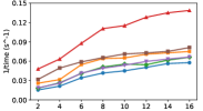
5.2.2 Scalability Comparison
We vary the number of nodes used in the cluster from 2 to 16 and record the average time for 100 iterations of each algorithm. Fig. 3 shows the reciprocal of per-iteration time as a function of the number of nodes used. All algorithms exhibit good scalability for all datasets (nearly a straight line), except for FACE (i.e., Fig. 3(a)). FACE is the smallest dataset, whose number of columns is 300, while is set to 100 by default. When is smaller than , the complexity is dominated by , hence, increasing the number of nodes does not reduce the computational cost, but may increase the communication overhead. In general, we can observe that DSANLS/Subsampling has the lowest per-iteration cost compared to all other algorithms, and DSANLS/Gaussian has similar cost to MU and HALS. ANLS/BPP has the highest per-iteration cost, explaining the bad performance of ANLS/BPP in Fig. 2.
5.2.3 Performance Varying the Value of
Although tuning the factorization rank is outside the scope of this paper, we compare the performance of DSANLS with MPI-FAUN varying the value of from 20 to 500 on RCV1. Observe from Fig. 4 and Fig. 2(e) () that DSANLS outperforms the state-of-art algorithms for all values of . Naturally, the relative error of all algorithms decreases with the increase of , but they also take longer to converge.
5.2.4 Comparison with Projected Gradient Descent
In Sec. 3.5, we claimed that our proximal coordinate descent approach (denoted as DSANLS-RCD) is faster than projected gradient descent (also presented in the same section, denoted as DSANLS-PGD). Fig. 5 confirms the difference in the convergence rate of the two approaches regardless of the random matrix generation approach.
5.3 Evaluation on Secure Distributed NMF
5.3.1 Performance Comparison for Uniform Workload
In Fig. 6, we show the relative error over time for secure distributed NMF algorithms on the 4 real public datasets, with a uniformly partition of columns. Syn-SSD-UV performs best in BOAT, FACE and GISETTE. As we will see in the next section, this is due to the fact that per-iteration cost of Syn-SSD-UV is significantly reduced by sketching. On MNIST, Syn-SSD-U and Syn-SSD-V has a better convergence in terms of relative error. Syn-SD and Asyn-SD converge relatively slowly and usually have a bad convergence result; on the other hand Asyn-SSD-V converges slowly but consistently generates better results than Syn-SD and Asyn-SD.
5.3.2 Performance Comparison for Imbalanced Workload
To evaluate the performance of different methods when the workload is imbalanced, we conduct experiments on skewed partition of input matrix. Among 10 worker nodes, node is assigned with of the columns, while other nodes have a uniform partition of the rest of columns. The measure for error is the same as the case of uniform workload.
It can be observed that in imbalanced workload, asynchronous algorithms generally outperform synchronous algorithms. Asyn-SSD-V gives the best result in terms of relative error over time, except dataset FACE. In FACE, Asyn-SD slowly converges to the best result. Unlike the case of uniform workload in Fig. 6, the sketching method Syn-SSD-UV does not perform well in imbalanced workload. Syn-SD are basically inapplicable in BOATS, MNIST and GISETTE datasets due to its slow speed. In sparse datasets MNIST and GISETTE, Syn-SSD-V and Syn-SSD-U can converge to a good result, but they do not generate satisfactory results on dense dataset BOATS and FACE.
5.3.3 Scalability Comparison
We vary the number of nodes used in the cluster from 2 to 16 and record the average time for 100 iterations of each algorithm. Fig. 8 shows the reciprocal of per-iteration time as a function of the number of nodes for uniform workload. All algorithms exhibit good scalability for all datasets (nearly a straight line), except for FACE (i.e., Fig. 8(b)). FACE is the smallest dataset, whose number of columns is 361 and number of row is 2,429. When is smaller than , the time consumed by subproblem solvers is dominated by the communication overhead. Hence, increasing the number of nodes is does not reduce per-iteration time. In general, we can observe that Syn-SSD-UV has the lowest per-iteration time compared to all other algorithms, and also has the best scalability as we can see from the steepest slope. Synchronous averaging has the highest per-iteration cost, explaining the bad performance in uniform workload experiments in Fig. 6.
In imbalanced workload settings, it is not surprising that asynchronous algorithms outperform synchronous algorithms with respect to scalability, as shown in Fig. 9. Synchronization barriers before All-Reduce operations severely affect the scalability of synchronous algorithms, resulting in a nearly flat curve for per-iteration time. The per-iteration time of Syn-SSD-UV is satisfactory when cluster size is small. However, it does not get significant improvements when more nodes are deployed. On the other hand, asynchronous algorithms demonstrate decent scalability as number of nodes grows. The short average iteration time of Asyn-SD and Asyn-SSD-V, shown in Fig. 9, also explains their superior performance over their synchronous counterparts in Fig. 7.
In conclusion, with an overall evaluation of convergence and scalability, Syn-SSD-UV should be adopted for secure distributed NMF under uniform workload, while Asyn-SSD-V is a more reasonable choice for secure distributed NMF under imbalanced workload.
6 Conclusion
In this paper, we studied the acceleration and security problems for distributed NMF. Firstly, we presented a novel distributed NMF algorithm DSANLS that can be used for scalable analytics of high dimensional matrix data. Our approach follows the general framework of ANLS, but utilizes matrix sketching to reduce the problem size of each NLS subproblem. We discussed and compared two different approaches for generating random matrices (i.e., Gaussian and subsampling random matrices). We presented two subproblem solvers for our general framework, and theoretically proved that our algorithm is convergent. We analyzed the per-iteration computational and communication cost of our approach and its convergence, showing its superiority compared to the state-of-the-art. Secondly, we designed four efficient distributed NMF methods in both synchronous and asynchronous settings with a security guarantee. They are the first distributed NMF methods over federated data, where data from all parties are utilized together in NMF for better performances and the data of each party remains confidential without leaking any individual information to other parties during the process. Finally, we conducted extensive experiments on several real datasets to show the superiority of our proposed methods. In the future, we plan to study the applications of DSANLS in dense or sparse tensors and consider more practical designs of asynchronous algorithm for secure distributed NMF.
7 Acknowledgment
This work was supported by the National Natural Science Foundation of China (no. 61972328).
Appendix A Proof of Lemma 1
Proof of Lemma 1.
Suppose is the global optimal solution but fails to satisfy Eq. 22 in the paper. If there exist indices such that , then
| (23) | ||||
However, simply choosing and will yield a smaller error , which contradicts the fact that is optimal. Therefore, if we define and , we must have for each . Now we construct a new solution by:
| (24) |
Note that
| (25) | ||||
so satisfy Eq. 22 in the paper. Besides,
| (26) | ||||
which means that is also an optimal solution. In short, for any optimal solution of Eq. 1 outside the domain shown in Eq. 22, there exists a corresponding global optimal solution satisfying the domain shown in Eq. 22, which further means that there exists at least one optimal solution in the domain shown in Eq. 22. ∎
Appendix B Proof of Theorem 1
For simplicity, we denote , , and . Let and denote the gradients of the above quantities, i.e.,
| (27) | ||||
Besides, let
| (28) |
B.1 Preliminary Lemmas
Lemma 2.
Lemma 3.
Assume is a nonnegative random variable with mean and variance , and is a constant. Then we have
| (29) |
Lemma 4.
Define the function
| (30) |
Conditioned on and , there exists an uniform constant such that
| (31) |
and
| (32) |
for any .
Lemma 5 (Supermartingale Convergence Theorem [52]).
Let , and , , be three sequences of random variables and let , , be sets of random variables such that . Suppose that
-
1.
The random variables , and are nonnegative, and are functions of the random variables in .
-
2.
For each , we have
(33) -
3.
There holds, with probability 1, .
Then we have , and the sequence converges to a nonnegative random variable , with probability 1.
Lemma 6 ([53]).
For two nonnegative scalar sequences and , if and , then
| (34) |
Furthermore, if for some constant , then
| (35) |
B.2 Proof of Theorem 1
Proof of Theorem 1.
Let us first focus on projected gradient descent. By conditioning on and , we have
| (36) |
For the second term of Eq. 36, note that
| (37) | ||||
By taking expectation and using Lemma 4, we obtain:
| (38) | ||||
For simplicity, we will use the notation
| (39) |
For the third term of Eq. 36, we can bound it in the following way:
| (40) | ||||
where in the last inequality we have applied Assumption 2. If we take expectation, we have
| (41) | ||||
where mean-variance decomposition have been applied in the second inequality, and Assumption 1 was used in the last line. For convenience, we will use
| (42) |
to denote this constant later on.
By combining all results, we can rewrite Eq. 36 as
| (43) |
Likewise, conditioned on and , we can prove a similar inequality for :
| (44) |
where is also some uniform constant. From definition, it is easy to see both and are nonnegative. Along with condition the condition , we can apply the Supermartingale Convergence Theorem (Lemma 5) with
| (45) | ||||
and then conclude that both and will converge to a same value, and besides:
| (46) |
with probability 1. In addition, it is not hard to verify that for some constant because of the boundness of the gradients. Then, by Lemma 6, we obtain that
| (47) |
Since each summand in the above is nonnegative, this equation further implies
| (48) |
for all and . By looking into the definition of in Eq. 30, it is not hard to see that if and only if . Considering and , we can conclude that
| (49) |
for all , which means either the gradient converges to , or converges to the boundary . In other words, the projected gradient at w.r.t converges to as . Likewise, we can prove
| (50) |
in a similar way, which completes the proof of projected gradient descent.
The proof of regularized coordinate descent is similar to that of projected gradient descent, and hence we only include a sketch proof here. The key here is to establish an inequality similar to Eq. 36, but with the difference that just one column rather than whole or is changed every time. Take as an example. An important observation is that when projection does not happen, we can rewrite (19) in the paper as , which means that the moving direction of regularized coordinate descent is the same as that of projected gradient descent, but with step size being . Since both the expectation and variance of are bounded, we will have when is large. Given these two reasons, we can out down a similar inequality as Eq. 36. The remaining proof just follows the one for projected gradient descent. ∎
B.3 Proof of Preliminary Lemmas
Proof of Lemma 2.
Since the proof related to is similar to , here we only focus on the latter one.
Proof of Lemma 3.
In this proof, we will use Cantelli’s inequality:
| (54) |
When , it is easy to see that the right-hand-side of Eq. 29 is . Considering that the left-hand-side is the expectation of a nonnegative random variable, Eq. 29 obviously holds in this case.
When and , by using the fact that is nonnegative, we have
| (55) |
Now we can apply Cantelli’s inequality to bound with , and obtain:
| (56) | ||||
where in the second inequality we used the fact again.
When but , we have:
| (57) |
Now we can apply inequality in Eq. 56 from the previous part with , and thus
| (58) |
which completes the proof. ∎
Proof of Lemma 4.
We only focus on and . We first show that
| (59) |
for any random matrix . Note that
| (60) | ||||
Hence it would be sufficient if we can show that there holds for any vectors and :
| (61) | ||||
where the first equality is because , the second equality is due to cyclic permutation invariant property of trace, and the last inequality is because all of , and are positive semi-definite matrices.
Now, let us consider the relationship between and :
| (62) |
from which it can be shown that
| (63) |
References
- Pauca et al. [2004] V. P. Pauca, F. Shahnaz, M. W. Berry, and R. J. Plemmons, “Text mining using non-negative matrix factorizations,” in SDM, 2004, pp. 452–456.
- Kotsia et al. [2007] I. Kotsia, S. Zafeiriou, and I. Pitas, “A novel discriminant non-negative matrix factorization algorithm with applications to facial image characterization problems,” IEEE Trans. Information Forensics and Security, vol. 2, no. 3-2, pp. 588–595, 2007.
- Gu et al. [2010] Q. Gu, J. Zhou, and C. H. Q. Ding, “Collaborative filtering: Weighted nonnegative matrix factorization incorporating user and item graphs,” in SDM, 2010, pp. 199–210.
- Zhang and Yeung [2012] Y. Zhang and D. Yeung, “Overlapping community detection via bounded nonnegative matrix tri-factorization,” in KDD, 2012, pp. 606–614.
- Kannan et al. [2016] R. Kannan, G. Ballard, and H. Park, “A high-performance parallel algorithm for nonnegative matrix factorization,” in PPOPP, 2016, pp. 9:1–9:11.
- Kim et al. [2017] Y. Kim, J. Sun, H. Yu, and X. Jiang, “Federated tensor factorization for computational phenotyping,” in KDD, 2017, pp. 887–895.
- Feng et al. [2018] J. Feng, L. T. Yang, Q. Zhu, and K.-K. R. Choo, “Privacy-preserving tensor decomposition over encrypted data in a federated cloud environment,” IEEE Trans. Dependable Sec. Comput., 2018.
- Kannan et al. [2018] R. Kannan, G. Ballard, and H. Park, “MPI-FAUN: an mpi-based framework for alternating-updating nonnegative matrix factorization,” IEEE Trans. Knowl. Data Eng., vol. 30, no. 3, pp. 544–558, 2018.
- Lee and Seung [2000] D. D. Lee and H. S. Seung, “Algorithms for non-negative matrix factorization,” in NIPS, 2000, pp. 556–562.
- Gillis [2014] N. Gillis, “The why and how of nonnegative matrix factorization,” arXiv Preprint, 2014. [Online]. Available: https://arxiv.org/abs/1401.5226
- Daube-Witherspoon and Muehllehner [1986] M. E. Daube-Witherspoon and G. Muehllehner, “An iterative image space reconstruction algorthm suitable for volume ect,” IEEE Trans. Med. Imaging, vol. 5, no. 2, pp. 61–66, 1986.
- Grippo and Sciandrone [2000] L. Grippo and M. Sciandrone, “On the convergence of the block nonlinear gauss-seidel method under convex constraints,” Oper. Res. Lett., vol. 26, no. 3, pp. 127–136, 2000.
- Kim and Park [2008] H. Kim and H. Park, “Nonnegative matrix factorization based on alternating nonnegativity constrained least squares and active set method,” SIAM J. Matrix Analysis Applications, vol. 30, no. 2, pp. 713–730, 2008.
- Kim and Park [2011] J. Kim and H. Park, “Fast nonnegative matrix factorization: An active-set-like method and comparisons,” SIAM J. Scientific Computing, vol. 33, no. 6, pp. 3261–3281, 2011.
- Lin [2007] C. Lin, “Projected gradient methods for nonnegative matrix factorization,” Neural Computation, vol. 19, no. 10, pp. 2756–2779, 2007.
- Zdunek and Cichocki [2006] R. Zdunek and A. Cichocki, “Non-negative matrix factorization with quasi-newton optimization,” in ICAISC, vol. 4029, 2006, pp. 870–879.
- Guan et al. [2012] N. Guan, D. Tao, Z. Luo, and B. Yuan, “Nenmf: An optimal gradient method for nonnegative matrix factorization,” IEEE Trans. Signal Processing, vol. 60, no. 6, pp. 2882–2898, 2012.
- Naor and Nissim [2001] M. Naor and K. Nissim, “Communication preserving protocols for secure function evaluation,” in STOC, 2001, pp. 590–599.
- Kanjani [2007] K. Kanjani, “Parallel non negative matrix factorization for document clustering,” CPSC-659 (Parallel and Distributed Numerical Algorithms) course. Texas A&M University, Tech. Rep, 2007.
- Robila and Maciak [2006] S. A. Robila and L. G. Maciak, “A parallel unmixing algorithm for hyperspectral images,” in Intelligent Robots and Computer Vision XXIV: Algorithms, Techniques, and Active Vision, vol. 6384, 2006, p. 63840F.
- Liu et al. [2010] C. Liu, H. Yang, J. Fan, L. He, and Y. Wang, “Distributed nonnegative matrix factorization for web-scale dyadic data analysis on mapreduce,” in WWW, 2010, pp. 681–690.
- Liao et al. [2014] R. Liao, Y. Zhang, J. Guan, and S. Zhou, “Cloudnmf: A mapreduce implementation of nonnegative matrix factorization for large-scale biological datasets,” Genomics, Proteomics & Bioinformatics, vol. 12, no. 1, pp. 48–51, 2014.
- Yin et al. [2014] J. Yin, L. Gao, and Z. M. Zhang, “Scalable nonnegative matrix factorization with block-wise updates,” in ECML/PKDD (3), ser. Lecture Notes in Computer Science, vol. 8726, 2014, pp. 337–352.
- Meng et al. [2016] X. Meng, J. K. Bradley, B. Yavuz, E. R. Sparks, S. Venkataraman, D. Liu, J. Freeman, D. B. Tsai, M. Amde, S. Owen, D. Xin, R. Xin, M. J. Franklin, R. Zadeh, M. Zaharia, and A. Talwalkar, “Mllib: Machine learning in apache spark,” J. Mach. Learn. Res., vol. 17, pp. 34:1–34:7, 2016.
- Grove et al. [2014] D. Grove, J. Milthorpe, and O. Tardieu, “Supporting array programming in X10,” in ARRAY@PLDI, 2014, pp. 38–43.
- Mejía-Roa et al. [2015] E. Mejía-Roa, D. Tabas-Madrid, J. Setoain, C. García, F. Tirado, and A. D. Pascual-Montano, “Nmf-mgpu: non-negative matrix factorization on multi-gpu systems,” BMC Bioinformatics, vol. 16, pp. 43:1–43:12, 2015.
- Gower and Richtárik [2015] R. M. Gower and P. Richtárik, “Randomized iterative methods for linear systems,” SIAM J. Matrix Analysis Applications, vol. 36, no. 4, pp. 1660–1690, 2015.
- Pilanci and Wainwright [2016] M. Pilanci and M. J. Wainwright, “Iterative hessian sketch: Fast and accurate solution approximation for constrained least-squares,” J. Mach. Learn. Res., vol. 17, pp. 53:1–53:38, 2016.
- Pilanci and Wainwright [2017] M. Pilanci and M. J. Wainwright, “Newton sketch: A near linear-time optimization algorithm with linear-quadratic convergence,” SIAM Journal on Optimization, vol. 27, no. 1, pp. 205–245, 2017.
- Wang and Li [2010] F. Wang and P. Li, “Efficient nonnegative matrix factorization with random projections,” in SDM, 2010, pp. 281–292.
- Lindell and Pinkas [2000] Y. Lindell and B. Pinkas, “Privacy preserving data mining,” in CRYPTO, vol. 1880, 2000, pp. 36–54.
- Wan et al. [2007] L. Wan, W. K. Ng, S. Han, and V. C. S. Lee, “Privacy-preservation for gradient descent methods,” in KDD, 2007, pp. 775–783.
- Han et al. [2010] S. Han, W. K. Ng, L. Wan, and V. C. S. Lee, “Privacy-preserving gradient-descent methods,” IEEE Trans. Knowl. Data Eng., vol. 22, no. 6, pp. 884–899, 2010.
- Pathak and Raj [2010] M. A. Pathak and B. Raj, “Privacy preserving protocols for eigenvector computation,” in PSDML, vol. 6549, 2010, pp. 113–126.
- Han et al. [2009] S. Han, W. K. Ng, and P. S. Yu, “Privacy-preserving singular value decomposition,” in ICDE, 2009, pp. 1267–1270.
- Chen et al. [2017] S. Chen, R. Lu, and J. Zhang, “A flexible privacy-preserving framework for singular value decomposition under internet of things environment,” in IFIPTM, vol. 505, 2017, pp. 21–37.
- Sakuma and Kobayashi [2010] J. Sakuma and S. Kobayashi, “Large-scale k-means clustering with user-centric privacy-preservation,” Knowl. Inf. Syst., vol. 25, no. 2, pp. 253–279, 2010.
- Lin and Jaromczyk [2011] Z. Lin and J. W. Jaromczyk, “Privacy preserving spectral clustering over vertically partitioned data sets,” in FSKD, 2011, pp. 1206–1211.
- Duan and Canny [2008] Y. Duan and J. F. Canny, “Practical private computation and zero-knowledge tools for privacy-preserving distributed data mining,” in SDM. SIAM, 2008, pp. 265–276.
- Beerliová-Trubíniová and Hirt [2008] Z. Beerliová-Trubíniová and M. Hirt, “Perfectly-secure MPC with linear communication complexity,” in TCC, vol. 4948, 2008, pp. 213–230.
- Damgård and Nielsen [2007] I. Damgård and J. B. Nielsen, “Scalable and unconditionally secure multiparty computation,” in CRYPTO, vol. 4622, 2007, pp. 572–590.
- Ailon and Chazelle [2006] N. Ailon and B. Chazelle, “Approximate nearest neighbors and the fast johnson-lindenstrauss transform,” in STOC, 2006, pp. 557–563.
- Lu et al. [2013] Y. Lu, P. S. Dhillon, D. P. Foster, and L. H. Ungar, “Faster ridge regression via the subsampled randomized hadamard transform,” in NIPS, 2013, pp. 369–377.
- Clarkson and Woodruff [2013] K. L. Clarkson and D. P. Woodruff, “Low rank approximation and regression in input sparsity time,” in STOC, 2013, pp. 81–90.
- Pham and Pagh [2013] N. Pham and R. Pagh, “Fast and scalable polynomial kernels via explicit feature maps,” in KDD, 2013, pp. 239–247.
- Nemirovski et al. [2009] A. Nemirovski, A. Juditsky, G. Lan, and A. Shapiro, “Robust stochastic approximation approach to stochastic programming,” SIAM J. on Optim., vol. 19, no. 4, pp. 1574–1609, 2009.
- Rockafellar [1976] R. T. Rockafellar, “Monotone operators and the proximal point algorithm,” SIAM J. Control Optim., vol. 14, no. 5, pp. 877–898, 1976.
- Fairbanks et al. [2015] J. P. Fairbanks, R. Kannan, H. Park, and D. A. Bader, “Behavioral clusters in dynamic graphs,” Parallel Computing, vol. 47, pp. 38–50, 2015.
- Qian et al. [2018] Y. Qian, C. Tan, N. Mamoulis, and D. W. Cheung, “DSANLS: accelerating distributed nonnegative matrix factorization via sketching,” in WSDM, 2018, pp. 450–458.
- Boyd et al. [2003] S. Boyd, L. Xiao, and A. Mutapcic, “Subgradient methods,” Stanford University, 2003. [Online]. Available: https://web.stanford.edu/class/ee392o/subgrad_method.pdf
- Kim et al. [2014] J. Kim, Y. He, and H. Park, “Algorithms for nonnegative matrix and tensor factorizations: a unified view based on block coordinate descent framework,” J. Global Optimization, vol. 58, no. 2, pp. 285–319, 2014.
- Neveu [1975] J. Neveu, Discrete-parameter martingales. Elsevier, 1975, vol. 10.
- Mairal [2013] J. Mairal, “Stochastic majorization-minimization algorithms for large-scale optimization,” in NIPS, 2013, pp. 2283–2291.
![[Uncaptioned image]](https://cdn.awesomepapers.org/papers/d6f7d086-38fa-49b5-8085-5739fb1ea536/yuqiu.jpg) |
Yuqiu Qian is currently an applied researcher in Tencent. Her research interests include data engineering and machine learning with applications in recommender systems. She received her B.Eng. degree in Computer Science from University of Science and Technology of China (2015), and her PhD degree in Computer Science from University of Hong Kong (2019). |
![[Uncaptioned image]](https://cdn.awesomepapers.org/papers/d6f7d086-38fa-49b5-8085-5739fb1ea536/conghui.jpg) |
Conghui Tan is currently a researcher in WeBank. His research interests include machine learning and optimization algorithms. He received his B.Eng. degree in Computer Science from University of Science and Technology of China (2015), and his PhD degree in System Engineering from Chinese University of Hong Kong (2019). |
![[Uncaptioned image]](https://cdn.awesomepapers.org/papers/d6f7d086-38fa-49b5-8085-5739fb1ea536/dan.jpg) |
Danhao Ding is currently a PhD candidate in Department of Computer Science, University of Hong Kong. His research interest include high performance computing and machine learning. He received his B.Eng. degree in Computing and Data Analytics from University of Hong Kong (2016). |
![[Uncaptioned image]](https://cdn.awesomepapers.org/papers/d6f7d086-38fa-49b5-8085-5739fb1ea536/hui.jpg) |
Hui Li is currently an assistant professor in the School of Informatics, Xiamen University. His research interests include data mining and data management with applications in recommender systems and knowledge graph. He received his B.Eng. degree in Software Engineering from Central South University (2012), and his MPhil and PhD degrees in Computer Science from University of Hong Kong (2015, 2018). |
![[Uncaptioned image]](https://cdn.awesomepapers.org/papers/d6f7d086-38fa-49b5-8085-5739fb1ea536/x37.png) |
Nikos Mamoulis received his diploma in computer engineering and informatics in 1995 from the University of Patras, Greece, and his PhD in computer science in 2000 from HKUST. He is currently a faculty member at the University of Ioannina. Before, he was professor at the Department of Computer Science, University of Hong Kong. His research focuses on the management and mining of complex data types. |