This paper was converted on www.awesomepapers.org from LaTeX by an anonymous user.
Want to know more? Visit the Converter page.

[2]\fnmChenglong \surBao

[2]\fnmZuoqiang \surShi

1]\orgdivDepartment of Mathematical Sciences, \orgnameTsinghua University, \orgaddress\streetHaidian District, \cityBeijing, \postcode100084, \stateBeijing, \countryChina

[2]\orgdivYau Mathematical Sciences Center, \orgnameTsinghua University, \orgaddress\streetHaidian District, \cityBeijing, \postcode100084, \stateBeijing, \countryChina

3]\orgdivBeijing Institute of Mathematical Sciences and Applications, \orgaddress\streetHuairou District, \cityBeijing, \postcode101408, \stateBeijing, \countryChina

Fast and Scalable Semi-Supervised Learning for Multi-View Subspace Clustering

\fnmHuaming \surLing [email protected]    [email protected]    \fnmJiebo \surSong [email protected]    [email protected] [ * [
Abstract

In this paper, we introduce a Fast and Scalable Semi-supervised Multi-view Subspace Clustering (FSSMSC) method, a novel solution to the high computational complexity commonly found in existing approaches. FSSMSC features linear computational and space complexity relative to the size of the data. The method generates a consensus anchor graph across all views, representing each data point as a sparse linear combination of chosen landmarks. Unlike traditional methods that manage the anchor graph construction and the label propagation process separately, this paper proposes a unified optimization model that facilitates simultaneous learning of both. An effective alternating update algorithm with convergence guarantees is proposed to solve the unified optimization model. Additionally, the method employs the obtained anchor graph and landmarks’ low-dimensional representations to deduce low-dimensional representations for raw data. Following this, a straightforward clustering approach is conducted on these low-dimensional representations to achieve the final clustering results. The effectiveness and efficiency of FSSMSC are validated through extensive experiments on multiple benchmark datasets of varying scales.

keywords:
Large-scale clustering, Multi-view subspace clustering, Semi-supervised clustering, Nonconvex optimization, Anchor graph learning

1 Introduction

Real-world datasets commonly encompass multi-view features that depict objects from different perspectives. For instance, materials conveying similar meanings might be expressed in different languages. The field of machine learning has seen the emergence of a significant topic known as multi-view clustering. This approach seeks to partition data by exploring consensus across multiple views. A prominent branch within this context is multi-view subspace clustering, which has garnered substantial attention during the last decade due to its promising performance [1, 2, 3, 4, 5, 6, 7, 8, 9, 10, 11, 12, 13, 14, 15]. These methodologies focus on acquiring self-representative affinity matrices by expressing each data point as a linear combination of all other data points in either the feature space or the latent space.

Despite the achievements of multi-view subspace clustering methods in various application domains, their application to large-scale datasets is hindered by significant time and memory overhead. These methods involve two primary phases: graph construction and spectral clustering. In the graph construction phase, the computational complexity of creating the self-representative affinity matrix for unstructured data is 𝒪(n3)\mathcal{O}(n^{3}), where nn denotes the data size. The subsequent spectral clustering phase incurs a computational complexity of at least 𝒪(n2)\mathcal{O}(n^{2}) due to the use of Singular Value Decomposition (SVD). Furthermore, the overall space complexity is estimated at 𝒪(n2)\mathcal{O}(n^{2}). In recent years, several landmark-based methods, as illustrated by [16, 17, 18], have emerged to enhance the efficiency of multi-view subspace clustering. These methods adopt an anchor graph strategy, generating a small number of landmarks (or anchors) and constructing anchor graphs to establish connections between the raw data and the landmarks. This anchor graph strategy significantly reduces computational and memory requirements, resulting in a linear complexity of 𝒪(n)\mathcal{O}(n), where nn denotes the data size.

In many applications, a small amount of supervisory information is often available despite the resource-intensive nature of data annotation. And several landmark-based semi-supervised learning methods like [19, 20, 21] have emerged to harness the available supervisory information. These methods encompass two core phases: anchor graph construction and label propagation. During anchor graph construction, an anchor graph is crafted by assessing similarities between raw data and landmarks. Subsequently, in label propagation, a graph structure is devised for landmarks with the previously derived anchor graph, confining the exploration of supervisory information to a much smaller graph and bypassing the complete graph construction for raw data. However, these methods handle anchor graph construction and label propagation in isolation. Consequently, the anchor graph’s formation occurs independently of supervisory information, potentially yielding a sub-optimal anchor graph that impairs label propagation. Moreover, their applicability is restricted to single-view datasets, precluding the utilization of multi-view features.

To address the above limitations of existing landmark-based semi-supervised learning methods, we introduce a novel method termed Fast Scalable Semi-supervised Multi-view Subspace Clustering (FSSMSC). This method formulates a unified optimization model aimed at concurrently facilitating the processes of anchor graph construction and label propagation. Notably, FSSMSC extends the landmark-based multi-view subspace clustering methods to harness supervisory information. Furthermore, the proposed FSSMSC offers a computational and space complexity of linear order with respect to the data size, rendering it applicable to large-scale datasets with multi-view features.

An efficient alternating update scheme is implemented to solve the proposed optimization model, cyclicly refreshing both the anchor graph and the landmarks’ low-dimensional representations. This iterative procedure facilitates simultaneous advancement in both the anchor graph and the low-dimensional representations of the landmarks. Significantly, within this iterative procedure, the consensus anchor graph undergoes updates utilizing both the data features and the landmarks’ representations, which contrasts with existing scalable semi-supervised learning methods such as [19, 20, 21] that solely construct the anchor graph based on data features. The landmarks’ representations act as pseudo supervision, facilitating the learning of the consensus anchor graph. While unsupervised clustering methods like [18] optimize anchor graph and landmarks simultaneously, they derive low-dimensional representations for clustering by employing Singular Value Decomposition (SVD) on the learned anchor graph, thereby handling anchor graph learning and low-dimensional representation learning separately. In contrast, our proposed semi-supervised learning method manages anchor graph construction and low-dimensional representation learning concurrently.

Our contributions can be summarized as follows:

  • We introduce a method termed Fast Scalable Semi-supervised Multi-view Subspace Clustering (FSSMSC), which extends the existing landmark-based multi-view subspace clustering methods to harness supervisory information. Moreover, the proposed FSSMSC offers linear computational and space complexity, making it well-suited for large-scale datasets with multi-view features.

  • Distinct from traditional methods that manage the anchor graph construction and the label propagation process separately, we formulate a unified optimization model that facilitates simultaneous learning of both.

  • An efficient alternating update scheme with convergence guarantees is introduced to solve the proposed optimization model, cyclicly updating both the anchor graph and the landmarks’ low-dimensional representations. Extensive experiments on multiple benchmark multi-view datasets of varying scales verify the efficiency and effectiveness of the proposed FSSMSC.

Notations. We denote matrices by boldface uppercase letters, e.g., 𝐙\mathbf{Z}, vectors by boldface lowercase letters, e.g., 𝐟\mathbf{f}, and scalars by lowercase letters, e.g., α\alpha. We denote zijz_{ij} or 𝐙ij\mathbf{Z}_{ij} as the (i,j)(i,j)-th element of 𝐙\mathbf{Z}. We use Tr(𝐙\mathbf{Z}) to denote the trace of any square matrix 𝐙\mathbf{Z}. |𝐙||\mathbf{Z}| is the matrix consisting of the absolute value of each element in 𝐙\mathbf{Z}. We denote diag(𝐖)\mbox{diag}(\mathbf{W}) as a vector of diagonal elements in 𝐖\mathbf{W} and diag(𝐟)\mbox{diag}(\mathbf{f}) as a diagonal matrix with 𝐟\mathbf{f} being the diagonal elements. 𝐖\mathbf{W}^{\top} is the transpose of 𝐖\mathbf{W}. We set 𝐈\mathbf{I} as the identity matrix and 𝟎\mathbf{0} as a matrix or vector of all zeros. We give the notations of some norms, e.g., 1\ell_{1}-norm 𝐙1=ij|zij|\|\mathbf{Z}\|_{1}=\sum_{ij}|z_{ij}| and Frobenius norm (or 2\ell_{2}-norm of a vector) 𝐙=ijzij2\|\mathbf{Z}\|=\sqrt{\sum_{ij}z_{ij}^{2}}.

2 Related Work

2.1 Subspace Clustering

Subspace clustering assumes that the data points are drawn from a union of multiple low-dimensional subspaces, with each group corresponding to one subspace. This clustering paradigm finds applications in diverse domains, including motion segmentation [22], face clustering [23], and image processing [24]. Within subspace clustering, self-representative subspace clustering achieves state-of-the-art performance by representing each data point as a linear combination of other data points within the same subspace. Such a representation is not unique, and sparse subspace clustering (SSC) [22] pursues a sparse representation by solving the following problem

min𝐙𝐙1+γ𝐗𝐗𝐙1,s.t.diag(𝐙)=𝟎,\displaystyle\min_{\mathbf{Z}}~{}\|\mathbf{Z}\|_{1}+\gamma\|\mathbf{X-XZ}\|_{1},~{}\text{s.t.}~{}\mbox{diag}(\mathbf{Z})=\mathbf{0}, (1)

where 𝐙\mathbf{Z} is a n×nn\times n self-representative matrix for nn data points 𝐗=[𝐱1,𝐱2,,𝐱n]\mathbf{X}=[\mathbf{x}_{1},\mathbf{x}_{2},\ldots,\mathbf{x}_{n}], and |𝐙ij||\mathbf{Z}_{ij}| reflects the affinity between data point 𝐱i\mathbf{x}_{i} and data point 𝐱j\mathbf{x}_{j}. Then the affinity matrix is induced by 𝐙\mathbf{Z} as 12(|𝐙|+|𝐙|)\frac{1}{2}\left(|\mathbf{Z}|+\left|\mathbf{Z}\right|^{\top}\right), which is further used for spectral clustering (SC) [25] to obtain the final clustering results.

In this paper, we represent each data point using selected landmarks to facilitate linear computational and space complexity relative to the data size nn.

2.2 Semi-Supervised Multi-View Learning

Owing to the prevalence of extensive real-world datasets with diverse features, numerous semi-supervised learning approaches have been developed specifically for multi-view data [26, 27, 28, 29, 30, 31, 32, 33]. The multiple graphs learning framework (AMGL) in [34] automatically learned the optimal weights for view-specific graphs. Additionally, the work [29] presented a multi-view learning with adaptive neighbors (MLAN) framework, concurrently performing label propagation and graph structure learning. [31] proposed a semi-supervised multi-view clustering method (GPSNMF) that constructs an affinity graph to preserve geometric information. An anti-block-diagonal indicator matrix was introduced in [32] to enforce the block-diagonal structure of the shared affinity matrix. [35] introduced a constrained tensor representation learning model to utilize prior weakly supervision for multi-view semi-supervised subspace clustering task. The work [33] proposed a novel semi-supervised multi-view clustering approach (CONMF) based on orthogonal non-negative matrix factorization. Despite their success in semi-supervised learning, these methods typically entail affinity matrix construction and exhibit at least 𝒪(n2)\mathcal{O}(n^{2}) computational complexity, where nn denotes the data size. Notably, a semi-supervised learning approach based on adaptive regression (MVAR) was introduced in [30], offering linear scalability with nn and quadratic scalability with feature dimension.

This paper introduces FSSMSC, a fast and scalable semi-supervised multi-view learning method to address the prevalent high computational complexity in existing approaches. FSSMSC exhibits linear computational and space complexity relative to data size and feature dimension.

3 Methodology

Table 1: Main notations
Notations Descriptions
nn Number of data points within the whole dataset
mm Number of selected landmarks
kk Number of clusters (categories)
nn_{\ell} Number of chosen labeled samples
𝐗(v)dv×n\mathbf{X}^{(v)}\in\mathbb{R}^{d_{v}\times n} Data matrix for the vv-th view
𝐔(v)dv×m\mathbf{U}^{(v)}\in\mathbb{R}^{d_{v}\times m} Data matrix of the selected mm landmarks for the vv-th view
𝐌,𝐂n×n\mathbf{M},\mathbf{C}\in\mathbb{R}^{n_{\ell}\times n_{\ell}} Matrices of pairwise constraints
𝐋𝐌,𝐋𝐂n×n\mathbf{L}_{\mathbf{M}},\mathbf{L}_{\mathbf{C}}\in\mathbb{R}^{n_{\ell}\times n_{\ell}} Laplacian matrices of 𝐌\mathbf{M} and 𝐂\mathbf{C}
𝐙m×n\mathbf{Z}\in\mathbb{R}^{m\times n} Consensus anchor graph
𝐀k×m\mathbf{A}\in\mathbb{R}^{k\times m} Low-dimensional representations of the selected mm landmarks

This section introduces the proposed Fast Scalable Semi-supervised Multi-view Subspace Clustering (FSSMSC) approach. We present the main notations of this paper in Table 1.

3.1 The Unified Optimization Model

For multi-view data, let VV denote the number of views, and 𝐗(v)dv×n\mathbf{X}^{(v)}\in\mathbb{R}^{d_{v}\times n} represent the data matrix for nn data points 𝐱1,𝐱2,,𝐱n\mathbf{x}_{1},\mathbf{x}_{2},\ldots,\mathbf{x}_{n} in the vv-th view, where dvd_{v} and nn stand for the dimension of the vv-th view and the data size, respectively. We perform kk-means clustering on the concatenated features of all views to establish consistent landmarks across all views. The resulting clustering centers are then partitioned into distinct views, denoted as 𝐔(v)dv×m\mathbf{U}^{(v)}\in\mathbb{R}^{d_{v}\times m}, v=1,,Vv=1,\dots,V. Assuming the first nn_{\ell} data points are provided with labels, while the remaining data points remain unlabeled. The label assigned to 𝐱i\mathbf{x}_{i} is denoted as i{1,,k}\ell_{i}\in\{1,\ldots,k\}, i=1,,ni=1,\ldots,n_{\ell}, where kk is the number of data categories. We formulate a more flexible form of supervisory information for the nn_{\ell} labeled data points, i.e., pairwise constraints ={(i,j)|i=j}\mathcal{M}=\{(i,j)|\ell_{i}=\ell_{j}\} and 𝒞={(i,j)|ij}\mathcal{C}=\{(i,j)|\ell_{i}\neq\ell_{j}\}, where \mathcal{M} and 𝒞\mathcal{C} denote the sets of data pairs subject to must-link and cannot-link constraints, respectively.

Scalable semi-supervised learning methods like [19, 20, 21] compute the soft label vectors for nn data points by a linear combination of the soft label vectors of mm chosen landmarks (anchors), where mm is notably smaller than nn. Similarly, we compute low-dimensional representations 𝐅k×n\mathbf{F}\in\mathbb{R}^{k\times n} for nn data points through a linear combination of low-dimensional representations 𝐀k×m\mathbf{A}\in\mathbb{R}^{k\times m} of mm landmarks

𝐟i=j=1m𝐙ji𝐚j,i=1,,n,\displaystyle\mathbf{f}_{i}=\sum\nolimits_{j=1}^{m}\mathbf{Z}_{ji}\mathbf{a}_{j},~{}~{}~{}i=1,\ldots,n, (2)

where 𝐟i\mathbf{f}_{i} is the ii-th column of 𝐅\mathbf{F}, 𝐚j\mathbf{a}_{j} is the jj-th column of 𝐀\mathbf{A}. Here, kk signifies the dimension of the low-dimensional space, consistently set as the number of data categories throughout this paper. Additionally, 𝐙=(𝐙ji)m×n\mathbf{Z}=(\mathbf{Z}_{ji})\in\mathbb{R}^{m\times n} is a consensus anchor graph capturing the relationships (similarities) between nn data points and mm selected landmarks.

However, these previous methods in [19, 20, 21] treat anchor graph learning and the learning of landmarks’ soft label vectors as disjoint sub-problems. In contrast, we formulate a unified optimization model facilitating concurrent advancement in both the anchor graph 𝐙\mathbf{Z} and the low-dimensional representations 𝐀\mathbf{A} of the landmarks. Specifically, the proposed unified optimization model of the anchor graph 𝐙\mathbf{Z} and low-dimensional representations 𝐀\mathbf{A} is based on the following observations.

Firstly, each entry 𝐙ji\mathbf{Z}_{ji} within the anchor graph 𝐙\mathbf{Z} should capture the affinity between the ii-th data point and the jj-th landmark. To fulfill this requirement, we extend the optimization model in (1) to a landmark-based multi-view clustering scenario. As discussed in Section 2.1, the optimization model (1) proposed in [22] represents each data point as a sparse linear combination of other data points within the same subspace, and induces the affinity matrix using these linear combination coefficients. Denote 𝐗(v)=[𝐱1(v),,𝐱n(v)]\mathbf{X}^{(v)}=[\mathbf{x}^{(v)}_{1},\dots,\mathbf{x}^{(v)}_{n}], where 𝐱i(v)\mathbf{x}^{(v)}_{i} represents the feature vector of the ii-th data point 𝐱i\mathbf{x}_{i} in the vv-th view. In this paper, we depict each 𝐱i(v)\mathbf{x}_{i}^{(v)} as a linear combination of the landmarks 𝐔(v)\mathbf{U}^{(v)} and assume that the combination coefficients are shared across views. Therefore, we explore the relationship among views by assuming that the anchor graph 𝐙\mathbf{Z} is shared across views to capture their consensus. Furthermore, we enforce coefficient sparsity by utilizing the 1\ell_{1}-norm on 𝐙\mathbf{Z}, leading to the following optimization problem:

min𝐙0\displaystyle\min_{\mathbf{Z}\geq 0}~{} φ(𝐙)=12v=1V𝐗(v)𝐔(v)𝐙2+λZ𝐙1,\displaystyle\varphi(\mathbf{Z})=\frac{1}{2}\sum_{v=1}^{V}\|\mathbf{X}^{(v)}-\mathbf{U}^{(v)}\mathbf{Z}\|^{2}+\lambda_{Z}\|\mathbf{Z}\|_{1}, (3)

where we impose non-negativity constraints on the elements in 𝐙\mathbf{Z}. The parameter λZ>0\lambda_{Z}>0 governs the sparsity level in 𝐙\mathbf{Z}.

Secondly, the low-dimensional representations for the nn data points, denoted as 𝐅=𝐀𝐙\mathbf{F=AZ} following (2), need to conform to the provided pairwise constraints. Specifically, data points with must-link (cannot-link) constraints should exhibit similar (distinct) low-dimensional representations. To fulfill this requirement, we encode the pairwise constraints into two matrices, 𝐌=(mij)n×n\mathbf{M}=(m_{ij})\in\mathbb{R}^{n_{\ell}\times n_{\ell}} and 𝐂=(cij)n×n\mathbf{C}=(c_{ij})\in\mathbb{R}^{n_{\ell}\times n_{\ell}}, with elements defined as:

mij={1nm,if(i,j)0,otherwise,cij={1nc,if(i,j)𝒞0,otherwise\displaystyle m_{ij}=\begin{cases}\frac{1}{n_{m}},&\text{if}~{}(i,j)\in\mathcal{M}\\ 0,&\text{otherwise}\end{cases},~{}c_{ij}=\begin{cases}\frac{1}{n_{c}},&\text{if}~{}(i,j)\in\mathcal{C}\\ 0,&\text{otherwise}\end{cases} (4)

where nmn_{m} (ncn_{c}) is the total number of must-link (cannot-link) constraints in \mathcal{M} (𝒞\mathcal{C}). The matrix 𝐌\mathbf{M} represents prior pairwise similarity constraints among data points. The element mijm_{ij} functions as a reward factor, with a positive value indicating a constraint that data points ii and jj should be grouped into the same cluster. In contrast, the matrix 𝐂\mathbf{C} denotes prior pairwise dissimilarity constraints. The element cijc_{ij} acts as a penalty factor, where positive values suggest that data points ii and jj should be assigned to different clusters. To balance the influence of must-link and cannot-link constraints, we normalize the non-zero entries in 𝐌\mathbf{M} and 𝐂\mathbf{C} by nmn_{m} and ncn_{c}, respectively. Subsequently, we utilize mijm_{ij} and cijc_{ij} to measure intra-class and inter-class distances for labeled data points, respectively, in the low-dimensional space. Specifically, we ensure that data pairs in \mathcal{M} share similar low-dimensional representations through the minimization of

ϕ(𝐀,𝐙)\displaystyle\phi_{\mathcal{M}}(\mathbf{A},\mathbf{Z}) =i,j=1nmij2𝐀𝐳i𝐀𝐳j2\displaystyle=\sum\nolimits_{i,j=1}^{n_{\ell}}\frac{m_{ij}}{2}\|\mathbf{A}\mathbf{z}_{i}-\mathbf{A}\mathbf{z}_{j}\|^{2} (5)
=Tr(𝐀𝐙𝐋𝐌(𝐀𝐙)),\displaystyle=\operatorname{Tr}(\mathbf{AZ_{\ell}}\mathbf{L}_{\mathbf{M}}(\mathbf{AZ_{\ell}})^{\top}),

where 𝐙\mathbf{Z}_{\ell} is the first nn_{\ell} columns of 𝐙\mathbf{Z} and 𝐳i\mathbf{z}_{i} is any ii-th column of 𝐙\mathbf{Z}, 𝐋𝐌=𝐃𝐌𝐌\mathbf{L}_{\mathbf{M}}=\mathbf{D_{M}}-\mathbf{M}, where 𝐃𝐌\mathbf{D_{M}} is a diagonal degree matrix with the ii-diagonal element being j=1nmij\sum_{j=1}^{n_{\ell}}m_{ij}. Similarly, we ensure that data pairs in 𝒞\mathcal{C} exhibit distinct low-dimensional representations through the maximization of

ϕ𝒞(𝐀,𝐙)\displaystyle\phi_{\mathcal{C}}(\mathbf{A},\mathbf{Z}) =i,j=1ncij2𝐀𝐳i𝐀𝐳j2\displaystyle=\sum\nolimits_{i,j=1}^{n_{\ell}}\frac{c_{ij}}{2}\|\mathbf{A}\mathbf{z}_{i}-\mathbf{A}\mathbf{z}_{j}\|^{2} (6)
=Tr(𝐀𝐙𝐋𝐂(𝐀𝐙)),\displaystyle=\operatorname{Tr}(\mathbf{AZ_{\ell}}\mathbf{L}_{\mathbf{C}}(\mathbf{AZ_{\ell}})^{\top}),

where 𝐋𝐂=𝐃𝐂𝐂\mathbf{L}_{\mathbf{C}}=\mathbf{D_{C}}-\mathbf{C} and 𝐃𝐂\mathbf{D_{C}} is a diagonal degree matrix with the ii-diagonal element being j=1ncij\sum_{j=1}^{n_{\ell}}c_{ij}.

Algorithm 1 FSSMSC
Input: Data features 𝐗(v),v=1,,V\mathbf{X}^{(v)},v=1,...,V, landmarks 𝐔(v),v=1,,V\mathbf{U}^{(v)},v=1,...,V, pairwise constraints 𝐋𝐌,𝐋𝐂\mathbf{L_{M}},\mathbf{L_{C}}, and parameters λZ,β,λM\lambda_{Z},\beta,\lambda_{M}.
Initialize: 𝐁=(λ𝐈+v=1V𝐔(v)𝐔(v))1\mathbf{B}=(\lambda\mathbf{I}+\sum_{v=1}^{V}\mathbf{U}^{(v)^{\top}}\mathbf{U}^{(v)})^{-1} \cdot
(v=1V𝐔(v)𝐗(v))(\sum_{v=1}^{V}\mathbf{U}^{(v)^{\top}}\mathbf{X}^{(v)}), 𝐙=min(mZ,max(𝟎,𝐁λZλ))\mathbf{Z}=\min(m_{Z},\max(\mathbf{0},\mathbf{B}-\frac{\lambda_{Z}}{\lambda})), 𝐪=𝐙𝐙𝟏\mathbf{q=ZZ^{\top}1}, 𝐀=𝟎\mathbf{A=0}, and Λ=𝟎\Lambda=\mathbf{0}.
repeat
     Update 𝐀\mathbf{A} by solving the trace ratio problem (12);
     Update 𝐙\mathbf{Z} by the formula (15);
     Update 𝐪\mathbf{q} by the formula (18);
     Update 𝐁\mathbf{B} by the least-square solution (20);
     Update the multiplier Λ\Lambda by (21);
until converged
Output: 𝐀,𝐙,𝐁\mathbf{A,Z,B}.

Thirdly, the representations 𝐀\mathbf{A} of landmarks should exhibit smoothness on the graph structure of landmarks, signifying that landmarks with higher similarity ought to possess spatially close representations. This objective is commonly achieved through the application of manifold smoothing regularization. Specifically, for a symmetric similarity matrix 𝐖m×m\mathbf{W}\in\mathbb{R}^{m\times m} of mm chosen landmarks, the manifold smoothing regularization is given by

i,j=1m𝐖ij2𝐚i𝐃ii𝐚j𝐃jj2=Tr(𝐀(𝐈𝐃12𝐖𝐃12)𝐀),\displaystyle\sum_{i,j=1}^{m}\frac{\mathbf{W}_{ij}}{2}\|\frac{\mathbf{a}_{i}}{\sqrt{\mathbf{D}_{ii}}}-\frac{\mathbf{a}_{j}}{\sqrt{\mathbf{D}_{jj}}}\|^{2}=\text{Tr}\left(\mathbf{A}(\mathbf{I}-\mathbf{D}^{-\frac{1}{2}}\mathbf{W}\mathbf{D}^{-\frac{1}{2}})\mathbf{A}^{\top}\right), (7)

where 𝐃\mathbf{D} is the diagonal degree matrix with 𝐃ii=j=1m𝐖ij\mathbf{D}_{ii}=\sum_{j=1}^{m}\mathbf{W}_{ij}. Minimizing this objective ensures that landmarks ii and jj with high similarity value 𝐖ij\mathbf{W}_{ij} have their scaled low-dimensional representations 𝐚i\mathbf{a}_{i} and 𝐚j\mathbf{a}_{j} close to each other.

Given that 𝐙ij0\mathbf{Z}_{ij}\geq 0 signifies the similarity between landmark ii and data point jj, we define the graph structure 𝐖\mathbf{W} for landmarks as 𝐖=𝐙𝐙\mathbf{W}=\mathbf{Z}\mathbf{Z}^{\top}, consistent with the definition in prior literature [20, 21]. We subsequently derive the normalized Laplacian matrix 𝐋𝐖\mathbf{L}_{\mathbf{W}} using 𝐋𝐖=𝐈𝐃12𝐖𝐃12\mathbf{L}_{\mathbf{W}}=\mathbf{I}-\mathbf{D}^{-\frac{1}{2}}\mathbf{W}\mathbf{D}^{-\frac{1}{2}}. Then, we introduce the manifold smoothing regularization as follows:

ϕs(𝐀,𝐙)=\displaystyle\phi_{s}(\mathbf{A},\mathbf{Z})= Tr(𝐀𝐋𝐖𝐀)\displaystyle\text{Tr}\left(\mathbf{A}\mathbf{L_{W}}\mathbf{A}^{\top}\right)
=\displaystyle= Tr(𝐀(𝐈𝐃𝐙1/2𝐙𝐙𝐃𝐙1/2)𝐀),\displaystyle\text{Tr}\left(\mathbf{A}(\mathbf{I}-\mathbf{D_{Z}}^{-1/2}\mathbf{Z}\mathbf{Z}^{\top}\mathbf{D_{Z}}^{-1/2})\mathbf{A}^{\top}\right), (8)

where 𝐃𝐙=diag(𝐙𝐙𝟏m)\mathbf{D_{Z}}=\text{diag}(\mathbf{Z}\mathbf{Z}^{\top}\mathbf{1}_{m}) and 𝟏m=(1,,1)m\mathbf{1}_{m}=(1,\cdots,1)^{\top}\in\mathbb{R}^{m}.

By consolidating the aforementioned optimization requirements, we establish a unified optimization problem for the simultaneous learning of 𝐙\mathbf{Z} and 𝐀\mathbf{A} as follows:

min𝐀,𝐙\displaystyle\min_{\mathbf{A},~{}\mathbf{Z}}~{} φ(𝐙)+βϕs(𝐀,𝐙)+λMϕ(𝐀,𝐙)ϕ𝒞(𝐀,𝐙)\displaystyle\varphi(\mathbf{Z})+\beta\cdot\frac{\phi_{s}(\mathbf{A},\mathbf{Z})+\lambda_{M}\phi_{\mathcal{M}}(\mathbf{A},\mathbf{Z})}{\phi_{\mathcal{C}}(\mathbf{A},\mathbf{Z})} (9)
s.t.𝐀𝐀=𝐈,𝐙0,\displaystyle\text{s.t.}~{}~{}\mathbf{A}\mathbf{A}^{\top}=\mathbf{I},~{}\mathbf{Z}\geq 0,

where β,λM>0\beta,\lambda_{M}>0 are penalty parameters.

We introduce auxiliary variable 𝐪m\mathbf{q}\in\mathbb{R}^{m} subject to the constraint 𝐪=𝐙𝐙𝟏m\mathbf{q}=\mathbf{Z}\mathbf{Z}^{\top}\mathbf{1}_{m}. Subsequently, we replace 𝐃𝐙\mathbf{D}_{\mathbf{Z}} with 𝐃𝐪=diag(𝐪)\mathbf{D_{q}}=\text{diag}(\mathbf{q}) in ϕs(𝐀,𝐙)\phi_{s}(\mathbf{A},\mathbf{Z}), denoted as ϕ~s(𝐀,𝐙,𝐪)\tilde{\phi}_{s}(\mathbf{A},\mathbf{Z},\mathbf{q}). To facilitate numerical stability and convergence analysis, we impose an upper bound mZ>0m_{Z}>0 on the elements in 𝐙\mathbf{Z} and enforce upper bound Cq>0C_{q}>0 and lower bound ϵq>0\epsilon_{q}>0 on the elements in 𝐪\mathbf{q}. Additionally, a positive constant ϵ>0\epsilon>0 is added to the denominator in (9). Consequently, the optimization problem is formulated as follows:

min𝐀,𝐙,𝐪\displaystyle\min_{\mathbf{A},\mathbf{Z},\mathbf{q}}~{} φ(𝐙)+βϕ~s(𝐀,𝐙,𝐪)+λMϕ(𝐀,𝐙)ϕ𝒞(𝐀,𝐙)+ϵ\displaystyle\varphi(\mathbf{Z})+\beta\cdot\frac{\tilde{\phi}_{s}(\mathbf{A},\mathbf{Z},\mathbf{q})+\lambda_{M}\phi_{\mathcal{M}}(\mathbf{A},\mathbf{Z})}{\phi_{\mathcal{C}}(\mathbf{A},\mathbf{Z})+\epsilon} (10)
+λ02𝐪𝐙𝐙𝟏m2\displaystyle+\frac{\lambda_{0}}{2}\|\mathbf{q}-\mathbf{Z}\mathbf{Z}^{\top}\mathbf{1}_{m}\|^{2}
s.t.𝐀𝐀=𝐈,mZ𝐙0,Cq𝐪ϵq,\displaystyle\text{s.t.}~{}~{}\mathbf{A}\mathbf{A}^{\top}=\mathbf{I},~{}m_{Z}\geq\mathbf{Z}\geq 0,C_{q}\geq\mathbf{q}\geq\epsilon_{q},

where λ02𝐪𝐙𝐙𝟏m2\frac{\lambda_{0}}{2}\|\mathbf{q}-\mathbf{Z}\mathbf{Z}^{\top}\mathbf{1}_{m}\|^{2} is the penalized term for the constraint 𝐪=𝐙𝐙𝟏m\mathbf{q}=\mathbf{Z}\mathbf{Z}^{\top}\mathbf{1}_{m} and λ0>0\lambda_{0}>0 is a penalized parameter.

3.2 Numerical Algorithm

We employ the Alternating Direction Method of Multipliers (ADMM) approach to solve the optimization problem (10).

We introduce auxiliary variables 𝐁=𝐙\mathbf{B}=\mathbf{Z}, leading to the augmented Lagrangian expression as follows:

λ(𝐀,𝐙,𝐪,𝐁,Λ)\displaystyle\mathcal{L}_{\lambda}(\mathbf{A},\mathbf{Z},\mathbf{q},\mathbf{B},\Lambda) (11)
=\displaystyle= 12v=1V𝐗(v)𝐔(v)𝐁2+λZ𝐙1+(Λ,𝐁𝐙)\displaystyle\frac{1}{2}\sum_{v=1}^{V}\|\mathbf{X}^{(v)}-\mathbf{U}^{(v)}\mathbf{B}\|^{2}+\lambda_{Z}\|\mathbf{Z}\|_{1}+(\Lambda,\mathbf{B-Z})
+βTr(𝐀(𝐈𝐃𝐪1/2𝐙𝐙𝐃𝐪1/2)𝐀)Tr(𝐀𝐙𝐋𝐂(𝐀𝐙))+ϵ\displaystyle+\beta\cdot\frac{\text{Tr}\left(\mathbf{A}(\mathbf{I}-\mathbf{D_{q}}^{-1/2}\mathbf{Z}\mathbf{Z}^{\top}\mathbf{D_{q}}^{-1/2})\mathbf{A}^{\top}\right)}{\text{Tr}\left(\mathbf{A}\mathbf{Z_{\ell}}\mathbf{L}_{\mathbf{C}}(\mathbf{A}\mathbf{Z_{\ell}})^{\top}\right)+\epsilon}
+βλMTr(𝐀𝐙𝐋𝐌(𝐀𝐙))Tr(𝐀𝐙𝐋𝐂(𝐀𝐙))+ϵ+λ2𝐁𝐙2\displaystyle+\beta\cdot\frac{\lambda_{M}\text{Tr}\left(\mathbf{A}\mathbf{Z_{\ell}}\mathbf{L}_{\mathbf{M}}(\mathbf{A}\mathbf{Z_{\ell}})^{\top}\right)}{\text{Tr}\left(\mathbf{A}\mathbf{Z_{\ell}}\mathbf{L}_{\mathbf{C}}(\mathbf{A}\mathbf{Z_{\ell}})^{\top}\right)+\epsilon}+\frac{\lambda}{2}\|\mathbf{B-Z}\|^{2}
+λ02𝐪𝐙𝐙𝟏m2+S0(𝐀)+S1(𝐙)+S2(𝐪),\displaystyle+\frac{\lambda_{0}}{2}\|\mathbf{q}-\mathbf{Z}\mathbf{Z}^{\top}\mathbf{1}_{m}\|^{2}+\ell_{S_{0}}(\mathbf{A})+\ell_{S_{1}}(\mathbf{Z})+\ell_{S_{2}}(\mathbf{q}),

where Λ\Lambda is the Lagrange multiplier. The trade-off parameters λM\lambda_{M}, λZ\lambda_{Z}, and β\beta are utilized to harmonize various components. We define S0={𝐀k×m|𝐀𝐀=𝐈}S_{0}=\{\mathbf{A}\in\mathbb{R}^{k\times m}|\mathbf{A}\mathbf{A}^{\top}=\mathbf{I}\}, S1={𝐙m×n|mZ𝐙0}S_{1}=\{\mathbf{Z}\in\mathbb{R}^{m\times n}|m_{Z}\geq\mathbf{Z}\geq 0\} and S2={𝐪m|ϵq𝐪Cq}S_{2}=\{\mathbf{q}\in\mathbb{R}^{m}|\epsilon_{q}\leq\mathbf{q}\leq C_{q}\}, with their respective indicator functions denoted as S0()\ell_{S_{0}}(\cdot), S1()\ell_{S_{1}}(\cdot) and S2()\ell_{S_{2}}(\cdot). Throughout our experiments, we fix λ\lambda and λ0\lambda_{0} as 100100, mZm_{Z} as 11, CqC_{q} as nn, and ϵ\epsilon and ϵq\epsilon_{q} as 1×1051\times 10^{-5}.

In each iteration, we alternatingly minimize over 𝐀\mathbf{A}, 𝐙\mathbf{Z}, 𝐪\mathbf{q}, B and then take gradient ascent steps on the Lagrange multiplier. The minimizations over 𝐀,𝐙,𝐪,𝐁\mathbf{A,Z,q,B} hold the other variables fixed and use the most recent value of each variable.

\bullet Update of 𝐀\mathbf{A}. The sub-problem on optimizing 𝐀\mathbf{A} can be written as an equivalent form

max𝐀𝐀=𝐈Tr(𝐀𝐋d𝐀)Tr(𝐀𝐋f𝐀),\displaystyle\max_{\mathbf{AA}^{\top}=\mathbf{I}}~{}\frac{\text{Tr}\left(\mathbf{A}\mathbf{L}_{d}\mathbf{A}^{\top}\right)}{\text{Tr}\left(\mathbf{A}\mathbf{L}_{f}\mathbf{A}^{\top}\right)}, (12)

where 𝐋f=λM(𝐙𝐋𝐌𝐙)+𝐈𝐃𝐪1/2𝐙𝐙𝐃𝐪1/2\mathbf{L}_{f}=\lambda_{M}\left(\mathbf{Z}_{\ell}\mathbf{L}_{\mathbf{M}}\mathbf{Z}_{\ell}^{\top}\right)+\mathbf{I}-\mathbf{D}_{\mathbf{q}}^{-1/2}\mathbf{Z}\mathbf{Z}^{\top}\mathbf{D}_{\mathbf{q}}^{-1/2} and 𝐋d=𝐙𝐋𝐂𝐙+ϵk𝐈\mathbf{L}_{d}=\mathbf{Z}_{\ell}\mathbf{L}_{\mathbf{C}}\mathbf{Z}_{\ell}^{\top}+\frac{\epsilon}{k}\cdot\mathbf{I}. The trace ratio optimization problem (12) can be effectively addressed using ALGORITHM 4.1 presented in [36].

\bullet Update of 𝐙\mathbf{Z}. The sub-problem on optimizing 𝐙\mathbf{Z} can be written as follows:

min𝐙𝒮1P(𝐙):=βϕ~s(𝐀,𝐙,𝐪)+λMϕ(𝐀,𝐙)ϕ𝒞(𝐀,𝐙)+ϵ(Λ,𝐙)\displaystyle\min_{\mathbf{Z}\in\mathcal{S}_{1}}P(\mathbf{Z}):=\beta\cdot\frac{\tilde{\phi}_{s}(\mathbf{A},\mathbf{Z},\mathbf{q})+\lambda_{M}\phi_{\mathcal{M}}(\mathbf{A},\mathbf{Z})}{\phi_{\mathcal{C}}(\mathbf{A},\mathbf{Z})+\epsilon}-(\Lambda,\mathbf{Z})
+λZi,j𝐙ij+λ2𝐁𝐙2+λ02𝐪𝐙𝐙𝟏m2.\displaystyle+\lambda_{Z}\sum_{i,j}\mathbf{Z}_{ij}+\frac{\lambda}{2}\|\mathbf{B-Z}\|^{2}+\frac{\lambda_{0}}{2}\|\mathbf{q}-\mathbf{Z}\mathbf{Z}^{\top}\mathbf{1}_{m}\|^{2}. (13)

We employ a one-step projected gradient descent strategy to update 𝐙\mathbf{Z}. By deriving the gradient of P(𝐙)P(\mathbf{Z}) with respect to 𝐙\mathbf{Z}, we can obtain:

𝐙P(𝐙)=\displaystyle\nabla_{\mathbf{Z}}P(\mathbf{Z})= Λ+λ(𝐙𝐁)+λZ𝟏m×n\displaystyle-\Lambda+\lambda(\mathbf{Z-B})+\lambda_{Z}\mathbf{1}_{m\times n} (14)
+[β𝐀𝐀𝐙𝐋pc,𝟎m×(nn)]2βτ2𝐃𝐪1/2𝐀𝐀𝐃𝐪1/2𝐙\displaystyle+[\beta\mathbf{A}^{\top}\mathbf{A}\mathbf{Z}_{\ell}\mathbf{L}_{pc},\mathbf{0}_{m\times(n-n_{\ell})}]-\frac{2\beta}{\tau_{2}}\mathbf{D}_{\mathbf{q}}^{-1/2}\mathbf{A}^{\top}\mathbf{A}\mathbf{D}_{\mathbf{q}}^{-1/2}\mathbf{Z}
+λ0((𝐙𝐙𝟏m𝐪)𝟏m𝐙+𝟏m(𝐙𝐙𝟏m𝐪)𝐙),\displaystyle+\lambda_{0}\left(\left(\mathbf{ZZ}^{\top}\mathbf{1}_{m}-\mathbf{q}\right)\mathbf{1}_{m}^{\top}\mathbf{Z}+\mathbf{1}_{m}\left(\mathbf{ZZ}^{\top}\mathbf{1}_{m}-\mathbf{q}\right)^{\top}\mathbf{Z}\right),

where 𝐋pc=2λMτ2𝐋𝐌2τ1τ22𝐋𝐂\mathbf{L}_{pc}=\frac{2\lambda_{M}}{\tau_{2}}\mathbf{L}_{\mathbf{M}}-\frac{2\tau_{1}}{\tau_{2}^{2}}\mathbf{L}_{\mathbf{C}}, τ2=ϕ𝒞(𝐀,𝐙)+ϵ\tau_{2}=\phi_{\mathcal{C}}(\mathbf{A},\mathbf{Z})+\epsilon, and τ1=ϕ~s(𝐀,𝐙,𝐪)+λMϕ(𝐀,𝐙)\tau_{1}=\tilde{\phi}_{s}(\mathbf{A},\mathbf{Z},\mathbf{q})+\lambda_{M}\phi_{\mathcal{M}}(\mathbf{A},\mathbf{Z}). Then we update 𝐙\mathbf{Z} by

𝐙=min(mZ,max(𝟎,𝐙ηz𝐙P(𝐙))),\displaystyle\mathbf{Z}=\min(m_{Z},\max(\mathbf{0},\mathbf{Z}-\eta_{z}\nabla_{\mathbf{Z}}P(\mathbf{Z}))), (15)

where ηz\eta_{z} is the step size, consistently set as 1λ\frac{1}{\lambda} in this paper.

\bullet Update of 𝐪\mathbf{q}. The sub-problem on optimizing 𝐪\mathbf{q} can be written as follows:

min𝐪𝒮2Q(𝐪):=\displaystyle\min_{\mathbf{q}\in\mathcal{S}_{2}}Q(\mathbf{q}):= βϕ~s(𝐀,𝐙,𝐪)ϕ𝒞(𝐀,𝐙)+ϵ+λ02𝐪𝐙𝐙𝟏m2.\displaystyle\beta\cdot\frac{\tilde{\phi}_{s}(\mathbf{A},\mathbf{Z},\mathbf{q})}{\phi_{\mathcal{C}}(\mathbf{A},\mathbf{Z})+\epsilon}+\frac{\lambda_{0}}{2}\|\mathbf{q}-\mathbf{Z}\mathbf{Z}^{\top}\mathbf{1}_{m}\|^{2}. (16)

By deriving the gradient of Q(𝐪)Q(\mathbf{q}) with respect to 𝐪\mathbf{q}, we can obtain:

𝐪Q(𝐪)=\displaystyle\nabla_{\mathbf{q}}Q(\mathbf{q})= βτ2diag(𝐙𝐙diag(𝐪1/2)𝐀𝐀diag(𝐪3/2))\displaystyle\frac{\beta}{\tau_{2}}\text{diag}\left(\mathbf{ZZ}^{\top}\text{diag}(\mathbf{q}^{-1/2})\mathbf{A}^{\top}\mathbf{A}\text{diag}(\mathbf{q}^{-3/2})\right) (17)
+λ0(𝐪𝐙𝐙𝟏m).\displaystyle+\lambda_{0}(\mathbf{q}-\mathbf{ZZ}^{\top}\mathbf{1}_{m}).

Then we update 𝐪\mathbf{q} by

𝐪=min(Cq,max(ϵq,𝐪ηq𝐪Q(𝐪))),\displaystyle\mathbf{q}=\min(C_{q},\max(\epsilon_{q},\mathbf{q}-\eta_{q}\nabla_{\mathbf{q}}Q(\mathbf{q}))), (18)

where ηq\eta_{q} is the step size, consistently set as 1λ\frac{1}{\lambda} in this paper.

\bullet Update of 𝐁\mathbf{B}. The sub-problem on optimizing 𝐁\mathbf{B} is

min𝐁12v=1V𝐗(v)𝐔(v)𝐁2+(Λ,𝐁𝐙)+λ2𝐁𝐙2.\displaystyle\min_{\mathbf{B}}\frac{1}{2}\sum_{v=1}^{V}\|\mathbf{X}^{(v)}-\mathbf{U}^{(v)}\mathbf{B}\|^{2}+(\Lambda,\mathbf{B-Z})+\frac{\lambda}{2}\|\mathbf{B-Z}\|^{2}. (19)

The solution to the above least-square problem is

𝐁=(v=1V𝐔(v)𝐔(v)+λ𝐈)1(v=1V𝐔(v)𝐗(v)+λ𝐙Λ).\displaystyle\mathbf{B}=(\sum_{v=1}^{V}\mathbf{U}^{(v)^{\top}}\mathbf{U}^{(v)}+\lambda\mathbf{I})^{-1}(\sum_{v=1}^{V}\mathbf{U}^{(v)^{\top}}\mathbf{X}^{(v)}+\lambda\mathbf{Z}-\Lambda). (20)

Since 𝐔(v)dv×m\mathbf{U}^{(v)}\in\mathbb{R}^{d_{v}\times m}, 𝐗(v)dv×n\mathbf{X}^{(v)}\in\mathbb{R}^{d_{v}\times n}, the computational complexity of solving the least-square problem amounts to 𝒪(m3+m2n+v=1Vdvmn)\mathcal{O}(m^{3}+m^{2}n+\sum_{v=1}^{V}d_{v}mn).

\bullet Update of the Lagrange multiplier Λ\Lambda.

Λ\displaystyle\Lambda =Λ+λ(𝐁𝐙).\displaystyle=\Lambda+\lambda(\mathbf{B-Z}). (21)

The detailed procedure is summarized in Algorithm 1.

3.3 Clustering Label Inference

Upon obtaining the anchor graph 𝐙\mathbf{Z} and landmarks’ low-dimensional representations 𝐀\mathbf{A} from Algorithm 1, the low-dimensional representations for the nn data points are computed as 𝐅=𝐀𝐙=[𝐟1,𝐟2,,𝐟n]\mathbf{F=AZ}=[\mathbf{f}_{1},\mathbf{f}_{2},\ldots,\mathbf{f}_{n}]. Subsequently, the cluster label cic_{i} for each data point 𝐱i,i=1,2,,n\mathbf{x}_{i},i=1,2,\ldots,n, is inferred using

ci=idx,idx=argminj{1,2,,n}𝐟i𝐟j.\displaystyle c_{i}=\ell_{idx},~{}~{}~{}idx=\mathop{\arg\min}\limits_{j\in\{1,2,\ldots,n_{\ell}\}}\|\mathbf{f}_{i}-\mathbf{f}_{j}\|. (22)

3.4 Complexity Analysis

We begin by conducting a computational complexity analysis of the proposed FSSMSC. For updating 𝐙\mathbf{Z}, the complexity is 𝒪(m2n+mn2)\mathcal{O}(m^{2}n+mn_{\ell}^{2}). The update of 𝐪\mathbf{q} involves a complexity of 𝒪(m2n)\mathcal{O}(m^{2}n). The complexity of updating 𝐀\mathbf{A} is 𝒪(m2n+mn2+m3)\mathcal{O}(m^{2}n+mn_{\ell}^{2}+m^{3}), while updating 𝐁\mathbf{B} requires 𝒪(dmn+m3+m2n)\mathcal{O}(dmn+m^{3}+m^{2}n), where dd stands for the total dimension of all features. The updates for Λ\Lambda incur a complexity of 𝒪(mn)\mathcal{O}(mn). Therefore, the overall computational complexity of FSSMSC amounts to 𝒪(m2n+mn2+m3+dmn)\mathcal{O}(m^{2}n+mn_{\ell}^{2}+m^{3}+dmn). Moving on to the space complexity evaluation, considering matrices such as 𝐗(v)dv×n\mathbf{X}^{(v)}\in\mathbb{R}^{d_{v}\times n}, 𝐔(v)dv×m\mathbf{U}^{(v)}\in\mathbb{R}^{d_{v}\times m} for v=1,,Vv=1,...,V, 𝐋𝐌,𝐋𝐂n×n\mathbf{L_{M}},\mathbf{L_{C}}\in\mathbb{R}^{n_{\ell}\times n_{\ell}}, 𝐙,𝐁,Λm×n\mathbf{Z,B},\Lambda\in\mathbb{R}^{m\times n}, and 𝐀k×m\mathbf{A}\in\mathbb{R}^{k\times m}, the aggregate space complexity totals 𝒪(dn+n2+mn+kn)\mathcal{O}(dn+n_{\ell}^{2}+mn+kn).

In summary, the proposed method demonstrates linear complexity, both in computation and space, with respect to the data size nn.

3.5 Convergence Analysis

We denote {𝐀k,𝐙k,𝐪k,𝐁k,Λk}\{\mathbf{A}^{k},\mathbf{Z}^{k},\mathbf{q}^{k},\mathbf{B}^{k},\Lambda^{k}\} as the variables generated by Algorithm 1 at iteration kk, and establish convergence guarantees for Algorithm 1.

Lemma 1.

Let h(𝐁)=12v=1V𝐗(v)𝐔(v)𝐁2h(\mathbf{B})=\frac{1}{2}\sum_{v=1}^{V}\|\mathbf{X}^{(v)}-\mathbf{U}^{(v)}\mathbf{B}\|^{2} and P,QP,Q are given in (3.2) and (16). Then 𝐁h(𝐁)\nabla_{\mathbf{B}}h(\mathbf{B}) is Lipschitz continuous with a Lipschitz constant Lh>0L_{h}>0. 𝐙P(𝐙)\nabla_{\mathbf{Z}}P(\mathbf{Z}) is Lipschitz continuous in 𝒮1\mathcal{S}_{1} with a Lipschitz constant L^Z>0\hat{L}_{Z}>0. 𝐪Q(𝐪)\nabla_{\mathbf{q}}Q(\mathbf{q}) is Lipschitz continuous in 𝒮2\mathcal{S}_{2} with a Lipschitz constant L^q>0\hat{L}_{q}>0.

Theorem 1.

If λ>Lh+2+2Lh2\lambda>L_{h}+2+2L_{h}^{2}, ηq<1L^q\eta_{q}<\frac{1}{\hat{L}_{q}}, and ηz<1L^Z\eta_{z}<\frac{1}{\hat{L}_{Z}}, the following properties hold:

(1) λ(𝐀k,𝐙k,𝐪k,𝐁k,Λk)\mathcal{L}_{\lambda}(\mathbf{A}^{k},\mathbf{Z}^{k},\mathbf{q}^{k},\mathbf{B}^{k},\Lambda^{k}) in (11) is lower bounded;

(2) There exists a constant C>0C>0 such that

λ(𝐀k,𝐙k,𝐪k,𝐁k,Λk)λ(𝐀k+1,𝐙k+1,𝐪k+1,𝐁k+1,Λk+1)\displaystyle\mathcal{L}_{\lambda}(\mathbf{A}^{k},\mathbf{Z}^{k},\mathbf{q}^{k},\mathbf{B}^{k},\Lambda^{k})-\mathcal{L}_{\lambda}(\mathbf{A}^{k+1},\mathbf{Z}^{k+1},\mathbf{q}^{k+1},\mathbf{B}^{k+1},\Lambda^{k+1})
\displaystyle\geq C(𝐁k+1𝐁k2+𝐪k+1𝐪k2),k;\displaystyle C\left(\|\mathbf{B}^{k+1}-\mathbf{B}^{k}\|^{2}+\|\mathbf{q}^{k+1}-\mathbf{q}^{k}\|^{2}\right),\forall k\in\mathbb{N}; (23)

(3) When kk\rightarrow\infty, we have

𝐁k+1𝐁k0,𝐙k+1𝐙k0,\displaystyle\|\mathbf{B}^{k+1}-\mathbf{B}^{k}\|\rightarrow 0,~{}~{}\|\mathbf{Z}^{k+1}-\mathbf{Z}^{k}\|\rightarrow 0,
Λk+1Λk0,𝐪k+1𝐪k0.\displaystyle\|\Lambda^{k+1}-\Lambda^{k}\|\rightarrow 0,~{}~{}\|\mathbf{q}^{k+1}-\mathbf{q}^{k}\|\rightarrow 0. (24)

The proofs for the aforementioned lemma and theorem are available in the appendix.

Table 2: Statistics of the datasets
Dataset #\#Samples #\#Views #\#Categories
Caltech7 1,474 6 7
HW 2,000 6 10
Caltech20 2,386 6 20
Reuters 18,758 5 6
NUS 30,000 5 31
Caltech101 9,144 6 102
YoutubeFace_\_sel 101,499 5 31

4 Experiments

Table 3: Comparison of clustering performance and running time. The best results are highlighted in boldface, and the second-best results are underlined. OM means Out-of-Memory.
Dataset FPMVS LMVSC MVAR MLAN AMGL GPSNMF CONMF FSSMSC
ACC(%\%)
Caltech7 57.1 70.6 91.7 ±\pm 1.7 91.6 ±\pm 2.4 85.3 ±\pm 1.6 93.1 ±\pm 1.5 92.7 ±\pm 1.6 93.7 ±\pm 1.9
HW 82.3 89.4 95.6 ±\pm 2.0 97.3 ±\pm 0.2 86.1 ±\pm 2.3 97.1 ±\pm 0.8 97.0 ±\pm 0.5 97.1 ±\pm 0.5
Caltech20 66.4 48.8 78.9 ±\pm 1.8 78.1 ±\pm 2.2 68.4 ±\pm 3.4 80.8 ±\pm 1.4 80.0 ±\pm 1.2 82.4 ±\pm 1.8
Reuters 57.5 49.6 OM OM 63.1 ±\pm 1.7 73.1 ±\pm 1.3 75.0 ±\pm 1.0 75.8 ±\pm 2.4
NUS 19.4 14.9 25.5 ±\pm 1.8 OM 19.1 ±\pm 1.3 28.3 ±\pm 1.0 24.8 ±\pm 1.0 29.2 ±\pm 1.6
Caltech101 28.8 25.6 44.3 ±\pm 0.8 45.2 ±\pm 0.6 39.6 ±\pm 1.0 43.1 ±\pm 0.8 47.3 ±\pm 0.8 47.1 ±\pm 0.8
Youtube111Youtube is an abbreviation of the dataset YoutubeFace_\_sel. 24.1 24.8 OM OM OM 39.9 ±\pm 2.0 OM 42.3 ±\pm 0.6
NMI (%\%)
Caltech7 55.6 48.1 78.3 ±\pm 3.8 79.7 ±\pm 3.5 66.4 ±\pm 2.7 82.6 ±\pm 3.5 81.2 ±\pm 2.1 84.3 ±\pm 4.2
HW 79.2 83.7 91.7 ±\pm 1.1 94.2 ±\pm 0.5 86.0 ±\pm 2.6 93.7 ±\pm 1.2 93.3 ±\pm 0.8 93.4 ±\pm 1.0
Caltech20 63.9 59.5 67.4 ±\pm 2.6 68.6 ±\pm 2.6 56.5 ±\pm 3.7 72.6 ±\pm 1.7 69.9 ±\pm 1.6 74.6 ±\pm 1.5
Reuters 35.9 35.6 OM OM 36.3 ±\pm 2.4 47.0 ±\pm 2.0 49.7 ±\pm 0.9 50.9 ±\pm 2.7
NUS 13.5 12.5 12.2 ±\pm 1.0 OM 6.7 ±\pm 1.1 14.4 ±\pm 0.6 13.0 ±\pm 0.2 17.7 ±\pm 1.0
Caltech101 41.8 48.5 41.5 ±\pm 0.8 46.1 ±\pm 0.8 38.1 ±\pm 0.8 44.0 ±\pm 0.7 50.9 ±\pm 0.5 50.9 ±\pm 0.6
Youtube 24.5 22.2 OM OM OM 26.8 ±\pm 1.6 OM 27.6 ±\pm 0.6
ARI (%\%)
Caltech7 41.3 43.0 87.6 ±\pm 4.1 85.4 ±\pm 6.0 65.4 ±\pm 4.1 92.6 ±\pm 3.0 92.4 ±\pm 2.1 93.6 ±\pm 4.1
HW 72.7 80.0 91.1 ±\pm 2.2 94.1 ±\pm 0.5 78.6 ±\pm 4.0 93.7 ±\pm 1.5 93.5 ±\pm 1.1 93.6 ±\pm 1.1
Caltech20 63.6 33.3 80.6 ±\pm 3.7 65.8 ±\pm 6.5 39.0 ±\pm 7.6 84.6 ±\pm 2.2 81.0 ±\pm 2.9 88.8 ±\pm 1.5
Reuters 33.2 22.1 OM OM 33.1 ±\pm 4.2 48.4 ±\pm 2.1 51.9 ±\pm 1.7 55.1 ±\pm 3.9
NUS 6.5 4.9 6.7 ±\pm 1.8 OM 2.8 ±\pm 1.6 10.8 ±\pm 0.7 10.7 ±\pm 0.5 13.8 ±\pm 2.2
Caltech101 17.4 19.1 41.5 ±\pm 2.4 35.7 ±\pm 3.5 20.6 ±\pm 3.3 39.2 ±\pm 1.9 63.5 ±\pm 1.8 63.8 ±\pm 1.2
Youtube 6.0 4.6 OM OM OM 7.8 ±\pm 2.1 OM 13.6 ±\pm 0.6
Running Time (ss)
Caltech7 23.2 251.7 4.6 10.9 0.9 8.4 12.9 2.8
HW 25.5 8.6 3.9 11.6 1.5 7.7 6.9 4.8
Caltech20 26.4 28.8 18.7 23.4 2.5 14.2 24.5 6.3
Reuters 1342.1 317.7 OM OM 326.3 1206.3 5096.6 109.5
NUS 1113.2 1879.4 763.9 OM 990.4 145.4 1431.4 40.7
Caltech101 684.9 2558.1 137.1 412.8 47.6 54.3 199.8 20.5
Youtube 3187.1 1152.7 OM OM OM 1128.4 OM 209.8

In this section, we conduct extensive experiments on seven benchmark multi-view datasets to evaluate the effectiveness and efficiency of the proposed method.

4.1 Experimental Settings

4.1.1 Datasets

We perform experiments on seven datasets widely employed for multi-view clustering: Handwritten (HW) [37], Caltech101 [38], Caltech7, Caltech20, Reuters [39], NUS-WIDE-Object (NUS) [40], and YoutubeFace_\_sel [41, 18]. Specifically, HW comprises 2,000 handwritten digits from 0 to 9. Caltech101 is an object recognition dataset including 9,144 data points. Caltech7 and Caltech20 are two widely-used subsets of Caltech101. Reuters includes documents in five languages and their translations; we use the English-written subset and its translations, which consists of 18,758 data points in 6 categories. NUS is also a dataset for object recognition, comprising 30,000 data points in 31 categories. YoutubeFace_\_sel is a video dataset containing 101,499 samples. The key dataset statistics are presented in Table 2.

4.1.2 Compared Methods

We compare the proposed FSSMSC with two scalable multi-view subspace clustering methods, including LMVSC [16] and FPMVS [18], and five state-of-the-art semi-supervised multi-view learning methods, including AMGL [34], MVAR [30], MLAN [29], GPSNMF [31], and CONMF [33].

4.1.3 Evaluation Metrics

We evaluate the clustering performance with clustering accuracy (ACC) [42], Normalized Mutual Information (NMI) [42], Adjusted Rand Index (ARI) [43], and running time in seconds. Since the proposed approach and the compared methods in the paper are implemented in MATLAB, we use the ”tic” and ”toc” functions to measure the elapsed time for each algorithm, with ”tic” marking the start and ”toc” marking the end of the execution of the algorithm. This elapsed time is reported as the algorithm’s running time.

4.1.4 Implementation Details

To ensure an equitable comparison, we acquired the released codes of the comparative methods and fine-tuned the parameters according to the corresponding papers to achieve optimal outcomes. In our approach, we consistently fix λ\lambda and λ0\lambda_{0} as 100100, mZm_{Z} as 11, CqC_{q} as nn, ϵ\epsilon and ϵq\epsilon_{q} as 1×1051\times 10^{-5}, and ηq\eta_{q} and ηz\eta_{z} as 1λ\frac{1}{\lambda}. Moreover, we select λM\lambda_{M} from {101,102,103,104,105}\{10^{1},10^{2},10^{3},10^{4},10^{5}\}, λZ\lambda_{Z} from {0.01,0.02,0.05,0.07,0.1,0.2,0.5}\{0.01,0.02,0.05,0.07,0.1,0.2,0.5\}, and β\beta from {105,104,103,102,101}\{10^{-5},10^{-4},10^{-3},10^{-2},10^{-1}\}. The number of clusters is set as the number of data categories kk. For LMVSC and FPMVS, the landmark number mm is explored from k,100,200,300,500{k,100,200,300,500}, with the best clustering performance reported. For the proposed FSSMSC, m=500m=500 is employed for most datasets, except for Caltech7 and Reuters, where m=300m=300 is selected. For AMGL, MLAN, MVAR, GPSNMF, CONMF, and FSSMSC, labeled samples constitute 5%5\% of the total samples for HW, Caltech7, Caltech20, and Caltech101, and 1%1\% for the larger datasets, Reuters, NUS and YoutubeFace_\_sel. Each experiment is repeated 20 times independently, and the average values and standard deviations are reported. All experiments are implemented in Matlab R2021a and run on a platform with a 2.10GHz Intel Xeon CPU and 128GB RAM.

4.2 Experimental Results and Discussion

Table 3 presents the clustering performance of different methods on the seven datasets. Based on the results depicted in Table 3, the following observations can be made:

  • Compared to the scalable multi-view subspace clustering methods, FPMVS and LMVSC, the proposed approach demonstrates a significant enhancement in clustering performance while utilizing a limited amount of supervisory information. For instance, FSSMSC exhibits improvements of 18.3%18.3\%, 9.8%9.8\%, and 17.5%17.5\% over datasets Reuters, NUS, and YoutubeFace_\_sel, respectively, for the ACC metric. Furthermore, FSSMSC notably outperforms FPMVS and LMVSC regarding running time.

  • In comparison to the semi-supervised multi-view learning methods (MVAR, MLAN, AMGL, GPSNMF, and CONMF), the proposed FSSMSC demonstrates comparable or superior performance with remarkably enhanced computational efficiency, particularly on large datasets such as YoutubeFace_\_sel, NUS, and Reuters. Specifically, FSSMSC demonstrates improvements of 5.8%5.8\%, 3.2%3.2\%, and 3.0%3.0\% in ARI metric on datasets YoutubeFace_\_sel, Reuters, and NUS, respectively, when contrasted with the five semi-supervised methods. Furthermore, FSSMSC exhibits computational efficiency advantages, running nearly 25 times faster than AMGL on NUS, 15 times faster than MVAR on NUS, 10 times faster than GPSNMF on Reuters, 20 times faster than MLAN on Caltech101, and 45 times faster than CONMF on Reuters.

  • When conducting experiments on the largest dataset, YoutubeFace_\_sel, the semi-supervised methods MVAR, MLAN, AMGL, and CONMF faced out-of-memory issues. The proposed FSSMSC demonstrates improvements of 2.4%2.4\% and 5.8%5.8\% over GPSNMF in terms of the ACC and ARI metrics, respectively, achieving this enhancement with significantly reduced running time.

These experiments verify the scalability, effectiveness, and efficiency of the proposed method.

Refer to caption
Figure 1: Clustering accuracy with different value of λM\lambda_{M} and β\beta on six datasets.
Refer to caption
Figure 2: Clustering accuracy with different value of λZ\lambda_{Z} on six datasets.
Refer to caption
Figure 3: The numerical convergence curves for six datasets, where the stopping criteria at iteration jj is defined as: StopC=max(𝐁j+1𝐁j,𝐙j+1𝐙j)\text{StopC}=\max(\|\mathbf{B}^{j+1}-\mathbf{B}^{j}\|_{\infty},\|\mathbf{Z}^{j+1}-\mathbf{Z}^{j}\|_{\infty}).

4.3 Sensitivity and Convergence Analysis

In Fig. 1 and Fig. 2, we conduct a sensitivity analysis for the three key parameters in FSSMSC, namely λZ\lambda_{Z}, λM\lambda_{M}, and β\beta, on six datasets. The following observations can be made from Fig. 1 and Fig. 2: (1) The parameter λZ\lambda_{Z}, governing the sparsity level of 𝐙\mathbf{Z}, significantly influences the clustering performance. Notably, the clustering accuracy exhibits more stable changes when the value of λZ\lambda_{Z} is relatively small; (2) Among the three relatively large datasets (Caltech101, NUS, and YoutubeFace_\_sel), higher values of λM\lambda_{M} such as 1×1051\times 10^{5} and smaller values of β\beta such as 1×1041\times 10^{-4} and 1×1031\times 10^{-3} are advantageous.

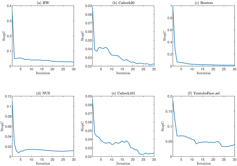
Additionally, numerical convergence curves for six datasets are presented in Fig. 3. It can be observed that the stopping criterion decreases rapidly in the initial five iterations and continues to decrease throughout the iterations. In our experiments, we set the maximum iteration number to 30.

4.4 Comparison of Semi-Supervised Methods under Different Labeled Ratios

We conduct experiments to assess the performance of our proposed method under different ratios of labeled samples. The results are presented in Fig. 4, Fig. 5, Fig. 6, and Fig. 7. The results are not included when an out-of-memory issue occurs. These results show that our proposed FSSMSC performs comparably to or better than semi-supervised competitors (MVAR, MLAN, AMGL, GPSNMF, and CONMF) across different labeled sample ratios. Additionally, as presented in Table 3, FSSMSC demonstrates notably reduced running times on the large datasets—NUS, Reuters, and YoutubeFace_\_sel. These results further validate the effectiveness of our approach.

Refer to caption
Figure 4: The evaluation metric ACC with different ratio of labeled samples on six datasets.
Refer to caption
Figure 5: The evaluation metric NMI with different ratio of labeled samples on six datasets.
Refer to caption
Figure 6: The evaluation metric ARI with different ratio of labeled samples on six datasets.
Refer to caption
Figure 7: The evaluation metrics with different ratio of labeled samples on the Caltech7 datasets.

4.5 Ablation Study

We conduct an ablation study for each component of our optimization model (9). The results are presented in Table 4. These ablation experiments include:

  • W/O 𝐙1\|\mathbf{Z}\|_{1}: Omitting the 1\ell_{1} norm of 𝐙\mathbf{Z} in φ(𝐙)\varphi(\mathbf{Z}), resulting in φ(𝐙)=12v=1V𝐗(v)𝐔(v)𝐙2\varphi(\mathbf{Z})=\frac{1}{2}\sum_{v=1}^{V}\|\mathbf{X}^{(v)}-\mathbf{U}^{(v)}\mathbf{Z}\|^{2}. Since 12v=1V𝐗(v)𝐔(v)𝐙2\frac{1}{2}\sum_{v=1}^{V}\|\mathbf{X}^{(v)}-\mathbf{U}^{(v)}\mathbf{Z}\|^{2} is a necessary component to utilize the data features 𝐗(v),v=1,,V\mathbf{X}^{(v)},v=1,\ldots,V, we preserve this part in φ(𝐙)\varphi(\mathbf{Z}).

  • W/O ϕ\phi_{\mathcal{M}}: Excluding the component ϕ(𝐀,𝐙)\phi_{\mathcal{M}}(\mathbf{A},\mathbf{Z}).

  • W/O ϕ𝒞\phi_{\mathcal{C}}: Omitting the component ϕ𝒞(𝐀,𝐙)\phi_{\mathcal{C}}(\mathbf{A},\mathbf{Z}).

  • W/O ϕs\phi_{s}: Excluding the component ϕs(𝐀,𝐙)\phi_{s}(\mathbf{A},\mathbf{Z}).

The results in Table 4 demonstrate that the full FSSMSC model consistently achieves superior clustering performance in most cases compared to versions with individual components removed. This confirms the importance and effectiveness of each component in our proposed model.

Table 4: The clustering metrics ACC and NMI on different datasets. The best results are highlighted in boldface.
Dataset Reuters NUS YoutubeFace_\_sel Caltech101 Caltech20 HW
ACC(%\%)
W/O 𝐙1\|\mathbf{Z}\|_{1} 68.1 ±\pm 2.3 29.2 ±\pm 1.2 34.5 ±\pm 0.6 38.5 ±\pm 0.6 75.8 ±\pm 1.5 89.5 ±\pm 1.9
W/O ϕ\phi_{\mathcal{M}} 64.4 ±\pm 2.4 20.8 ±\pm 0.9 35.9 ±\pm 0.8 43.4 ±\pm 0.6 80.5 ±\pm 1.5 96.9 ±\pm 0.6
W/O ϕ𝒞\phi_{\mathcal{C}} 69.5 ±\pm 1.9 17.1 ±\pm 1.3 24.7 ±\pm 0.9 44.8 ±\pm 0.7 82.2 ±\pm 1.7 97.1 ±\pm 0.5
W/O ϕs\phi_{s} 58.0 ±\pm 12.7 21.9 ±\pm 4.5 30.2 ±\pm 1.5 42.9 ±\pm 1.2 80.5 ±\pm 4.2 86.8 ±\pm 6.3
FSSMSC 75.8 ±\pm 2.4 29.2 ±\pm 1.6 42.3 ±\pm 0.6 47.1 ±\pm 0.8 82.4 ±\pm 1.8 97.1 ±\pm 0.5
NMI(%\%)
W/O 𝐙1\|\mathbf{Z}\|_{1} 41.3 ±\pm 2.4 17.2 ±\pm 1.0 21.2 ±\pm 0.7 42.8 ±\pm 0.6 64.7 ±\pm 1.4 82.5 ±\pm 1.5
W/O ϕ\phi_{\mathcal{M}} 37.0 ±\pm 2.6 11.0 ±\pm 0.5 21.1 ±\pm 0.6 47.3 ±\pm 0.5 72.3 ±\pm 1.4 93.2 ±\pm 1.2
W/O ϕ𝒞\phi_{\mathcal{C}} 44.2 ±\pm 2.0 7.6 ±\pm 0.9 9.7 ±\pm 0.5 47.8 ±\pm 0.7 75.1 ±\pm 1.3 93.6 ±\pm 0.9
W/O ϕs\phi_{s} 28.1 ±\pm 15.0 13.6 ±\pm 4.5 16.9 ±\pm 1.3 46.8 ±\pm 1.3 70.6 ±\pm 6.4 77.8 ±\pm 7.8
FSSMSC 50.9 ±\pm 2.7 17.7 ±\pm 1.0 27.6 ±\pm 0.6 50.9 ±\pm 0.6 74.6 ±\pm 1.5 93.4 ±\pm 1.0

Moreover, we perform an ablation study on the parameter β\beta. FSSMSC indicates the case where β\beta is fixed at 0 in Algorithm 1, while FSSMSC denotes the usage of a tuned non-zero β\beta. The principal distinction between FSSMSC and FSSMSC lies in the 𝐙\mathbf{Z} update. In FSSMSC, 𝐙\mathbf{Z} is updated without utilizing the landmarks’ representations 𝐀\mathbf{A}. Conversely, in FSSMSC, 𝐙\mathbf{Z} is updated using both data features and landmarks’ representations. Therefore, anchor graph learning in FSSMSC is decoupled from the label propagation process. The results of applying FSSMSC and FSSMSC to different datasets are presented in Table 5. The outcomes depicted in Table 5 illustrate that FSSMSC outperforms FSSMSC in terms of ACC and NMI metrics. This observation verifies the efficacy of the simultaneous learning of the anchor graph and label propagation.

Table 5: The clustering metrics ACC and NMI on different datasets. FSSMSC denotes the scenario where β\beta is set to 0 in Algorithm 1.
Dataset Reuters NUS YoutubeFace_\_sel Caltech101 HW
ACC(%\%)
FSSMSC 75.2 ±\pm 2.5 26.1 ±\pm 1.1 41.0 ±\pm 0.6 46.9 ±\pm 0.7 97.0 ±\pm 0.6
FSSMSC 75.8 ±\pm 2.4 29.2 ±\pm 1.6 42.3 ±\pm 0.6 47.1 ±\pm 0.8 97.1 ±\pm 0.5
NMI(%\%)
FSSMSC 49.9 ±\pm 2.8 14.7 ±\pm 0.6 26.1 ±\pm 0.5 50.4 ±\pm 0.6 93.3 ±\pm 1.0
FSSMSC 50.9 ±\pm 2.7 17.7 ±\pm 1.0 27.6 ±\pm 0.6 50.9 ±\pm 0.6 93.4 ±\pm 1.0

4.6 Relationship Between Computational Complexity and Running Time

In this section, we illustrate the relationship between the computational complexity and the growth speed of running time. For instance, the compared semi-supervised algorithms MLAN, AMGL, GPSNMF, and CONMF require constructing similarity matrices for all samples across all views. The computational complexity for constructing these similarity matrices is O(dn2)O(dn^{2}), where dd is the total feature dimension of all views and nn is the number of samples. This complexity scales quadratically with nn, whereas our algorithm’s overall complexity scales linearly with nn. Therefore, as nn increases, the running time required to construct these similarity matrices grows significantly faster for these methods compared to our approach.

We provide empirical evidence for this by reporting the total running time of the semi-supervised methods, as well as the running time required to construct similarity matrices before the iterative update procedure, across four datasets, as detailed in Table 6. In Table 6, values in parentheses denote the running time for similarity matrix construction, while those outside parentheses represent the total running time. It can be observed that as nn increases, the running time required to construct the similarity matrices (values in parentheses) grows significantly faster compared to our FSSMSC. For example, the data size of the YoutubeFace_\_sel dataset is nearly 3.4 times that of the NUS dataset, yet the running time for constructing similarity matrices for GPSNMF on the YoutubeFace_\_sel dataset (646.0 seconds) is nearly 15.3 times that of the NUS dataset (42.3 seconds). In contrast, the total running time of our algorithm on the YoutubeFace_\_sel dataset (209.8 seconds) is approximately 5.2 times that of the NUS dataset (40.7 seconds).

Notably, MVAR does not involve similarity matrix construction, and its computational complexity scales linearly with nn while quadratically with dd. Variations in running times for similarity matrix construction on the same dataset among MLAN, AMGL, GPSNMF, and CONMF are due to differences in their respective construction methods.

Table 6: The running time (in seconds) of each semi-supervised method. Values in parentheses denote the running time for similarity matrix construction, while those outside parentheses represent the total running time. Note that the MVAR and our FSSMSC methods do not involve constructing n×nn\times n similarity matrices. The best total running times are highlighted in boldface. OM means Out-of-Memory.
Dataset data size nn MVAR MLAN AMGL GPSNMF CONMF FSSMSC
Caltech20 2,386 18.7 23.4(1.4) 2.5(1.7) 14.2(0.6) 24.5(2.3) 6.3
Caltech101 9,144 137.1 412.8(20.8) 47.6(27.1) 54.3(4.1) 199.8(8.6) 20.5
NUS 30,000 763.9 OM 990.4(440.2) 145.4(42.3) 1431.4(105.5) 40.7
Youtube 101,499 OM OM OM 1128.4(646.0) OM 209.8
11footnotetext: Youtube is an abbreviation of the dataset YoutubeFace_\_sel.

4.7 The Floating Point Operations Evaluation

The proposed approach and the compared methods in the paper are implemented in MATLAB. However, MATLAB does not have an official function or program to report exact Floating Point Operations (FLOPs). We use a publicly available MATLAB program [44] to estimate the FLOPs on the four large datasets, as shown in Table 7. From Table 7, we can observe that our proposed FSSMSC achieves significantly fewer FLOPs compared to other semi-supervised competitors.

Table 7: The estimated Floating Point Operations (FLOPs) of the semi-supervised methods. The best results are in boldface. OM means Out-of-Memory.
Dataset MVAR MLAN AMGL GPSNMF CONMF FSSMSC
Caltech101 4.03×10134.03\times 10^{13} 1.06×10141.06\times 10^{14} 7.73×10127.73\times 10^{12} 1.32×10131.32\times 10^{13} 1.11×10131.11\times 10^{13} 6.20×𝟏𝟎𝟏𝟏\mathbf{6.20\times 10^{11}}
Reuters OM OM 1.03×10141.03\times 10^{14} 1.59×10141.59\times 10^{14} 5.41×10135.41\times 10^{13} 1.63×𝟏𝟎𝟏𝟐\mathbf{1.63\times 10^{12}}
NUS 6.76×10136.76\times 10^{13} OM 2.13×10142.13\times 10^{14} 1.02×10141.02\times 10^{14} 2.34×10132.34\times 10^{13} 1.86×𝟏𝟎𝟏𝟐\mathbf{1.86\times 10^{12}}
YoutubeFace_\_sel OM OM OM 1.18×10151.18\times 10^{15} OM 6.53×𝟏𝟎𝟏𝟐\mathbf{6.53\times 10^{12}}

It should be noted that while GPSNMF typically has more FLOPs than CONMF, it takes less running time. This discrepancy arises from the FLOPs calculation rules in the used program [44]. The program calculates the FLOPs of multiplying an n×pn\times p matrix 𝐀\mathbf{A} by a p×mp\times m matrix 𝐁\mathbf{B} as 2npm2npm, regardless of whether the matrix is represented as sparse or not. However, in the released codes of GPSNMF, the similarity matrix 𝐒p\mathbf{S}^{p} and its sub-matrix 𝐒up\mathbf{S}_{u}^{p} are represented in sparse format (encoding the row and column indexes for the nonzero elements). Therefore, the actual FLOPs of matrix multiplication with these matrices may be overestimated. This may explain why the running time of GPSNMF is less than that of CONMF.

Additionally, the semi-supervised competitors MLAN, AMGL, GPSNMF, and CONMF require constructing similarity matrices for all samples across all views before the iterative update procedure. The FLOPs for this process are estimated as dn2dn^{2}, where dd is the total feature dimension of all views and nn is the number of samples. The FLOPs for this process on the Caltech101, NUS, and YoutubeFace_\_sel datasets are shown in Table 8. On the YoutubeFace_\_sel dataset, the FLOPs for constructing similarity matrices (2.19×10132.19\times 10^{13}) is nearly 3.4 times of the FLOPs of our proposed FSSMSC (6.53×10126.53\times 10^{12}). Moreover, the FLOPs for constructing these similarity matrices scale quadratically with nn, whereas our approach scales linearly with nn. This means that the FLOPs of constructing similarity matrices for these methods grows significantly faster compared to our approach.

Table 8: The FLOPs of constructing n×nn\times n similarity matrices for all views.
Dataset Caltech101 NUS YoutubeFace_\_sel
data size nn 9,144 30,000 101,499
total dimension dd 3,766 639 2,125
dn2dn^{2} 3.15×10113.15\times 10^{11} 5.75×10115.75\times 10^{11} 2.19×10132.19\times 10^{13}

4.8 Experimental Validation of Linear Space Complexity

We conduct experiments to confirm the linear property of our algorithm’s space complexity. As illustrated in Table 9, we evaluate the space complexity by examining the memory usage of the variables in the MATLAB implementation of our algorithm. The Reuters dataset is not included due to its extremely high feature dimension compared to the other six datasets. The results show that the values of bytes/n for our approach are comparable across different datasets, indicating that the space complexity empirically scales linearly with the data size nn. Additionally, the observed fluctuations in the values of bytes/n are due to variations in feature dimensions and the number of selected landmarks across datasets.

Table 9: The memory usage (in bytes) of our approach on different datasets.
Dataset HW Caltech7 Caltech20 Caltech101 NUS YoutubeFace_\_sel
data size nn 2,000 1,474 2,386 9,144 30,000 101,499
total dimension dd 649 3,766 3,766 3,766 639 2,125
bytes 1.43×1081.43\times 10^{8} 1.10×1081.10\times 10^{8} 2.39×1082.39\times 10^{8} 8.26×1088.26\times 10^{8} 1.74×1091.74\times 10^{9} 7.05×1097.05\times 10^{9}
bytes/n 7.15×1047.15\times 10^{4} 7.46×1047.46\times 10^{4} 1.00×1051.00\times 10^{5} 9.03×1049.03\times 10^{4} 5.80×1045.80\times 10^{4} 6.95×1046.95\times 10^{4}

For comparison, since each element of the matrix consumes 8 bytes, the n×nn\times n similarity matrices for all five views of the YoutubeFace_\_sel dataset takes bytes of 5×101,499×101,499×8>4.12×10115\times 101,499\times 101,499\times 8>4.12\times 10^{11}, which is significantly large than the 7.05×1097.05\times 10^{9} bytes required by our approach. Furthermore, the memory usage for a full n×nn\times n similarity matrix grows quadratically with the data size nn, whereas the memory usage for our approach grows linearly with nn.

5 Conclusion

This paper introduces the Fast Scalable Semi-supervised Multi-view Subspace Clustering (FSSMSC) method, a novel approach addressing the prevalent high computational complexity in existing approaches. Importantly, FSSMSC offers linear computational and space complexity, rendering it suitable for large-scale multi-view datasets. Unlike conventional methods that manage anchor graph construction and label propagation independently, we propose a unified optimization model for simultaneously learning both components. Extensive experiments on seven multi-view datasets demonstrate the efficiency and effectiveness of the proposed method.

\bmhead

Acknowledgements

We appreciate the support by the National Natural Science Foundation of China (No.12271291, No.12071244, and No.92370125) and the National Key R&\&D Program of China (No.2021YFA1001300).

Appendix A Proofs of Lemma 1 and Theorem 1

We begin by presenting essential notations and definitions, followed by the proofs for Lemma 1 and Theorem 1 in the paper, denoted as Lemma 2 and Theorem 2 in this appendix.

Let 𝒮0={𝐀k×m|𝐀𝐀=𝐈}\mathcal{S}_{0}=\{\mathbf{A}\in\mathbb{R}^{k\times m}|\mathbf{A}\mathbf{A}^{\top}=\mathbf{I}\}, 𝒮1={𝐙m×n|mZ𝐙𝟎}\mathcal{S}_{1}=\{\mathbf{Z}\in\mathbb{R}^{m\times n}|m_{Z}\geq\mathbf{Z}\geq\mathbf{0}\}, and 𝒮2={𝐪m|Cq𝐪ϵq}\mathcal{S}_{2}=\{\mathbf{q}\in\mathbb{R}^{m}|C_{q}\geq\mathbf{q}\geq\epsilon_{q}\}, along with their indicator functions denoted as 𝒮0()\ell_{\mathcal{S}_{0}}(\cdot), 𝒮1()\ell_{\mathcal{S}_{1}}(\cdot), and 𝒮2()\ell_{\mathcal{S}_{2}}(\cdot).

Let h(𝐁)=12v=1V𝐗(v)𝐔(v)𝐁2h(\mathbf{B})=\frac{1}{2}\sum_{v=1}^{V}\|\mathbf{X}^{(v)}-\mathbf{U}^{(v)}\mathbf{B}\|^{2} and define the functions g(𝐀,𝐙,𝐪)g(\mathbf{A},\mathbf{Z},\mathbf{q}) and g0(𝐙,𝐪)g_{0}(\mathbf{Z},\mathbf{q}) as follows:

g(𝐀,𝐙,𝐪)\displaystyle g(\mathbf{A},\mathbf{Z},\mathbf{q}) =β(Tr(𝐀(𝐈𝐃𝐪1/2𝐙𝐙𝐃𝐪1/2)𝐀)+λMTr(𝐀𝐙𝐋𝐌𝐙𝐀))Tr(𝐀𝐙𝐋𝐂𝐙𝐀)+ϵ\displaystyle=\beta\cdot\frac{\left(\text{Tr}(\mathbf{A}(\mathbf{I}-\mathbf{D}_{\mathbf{q}}^{-1/2}\mathbf{ZZ}^{\top}\mathbf{D}_{\mathbf{q}}^{-1/2})\mathbf{A}^{\top})+\lambda_{M}\text{Tr}(\mathbf{A}\mathbf{Z}_{\ell}\mathbf{L}_{\mathbf{M}}\mathbf{Z}_{\ell}^{\top}\mathbf{A}^{\top})\right)}{\text{Tr}(\mathbf{A}\mathbf{Z}_{\ell}\mathbf{L}_{\mathbf{C}}\mathbf{Z}_{\ell}^{\top}\mathbf{A}^{\top})+\epsilon} (25)
g0(𝐙,𝐪)\displaystyle g_{0}(\mathbf{Z},\mathbf{q}) =λ02𝐪𝐙𝐙𝟏m2\displaystyle=\frac{\lambda_{0}}{2}\|\mathbf{q}-\mathbf{ZZ}^{\top}\mathbf{1}_{m}\|^{2}

Additionally, let

f0(𝐀)\displaystyle f_{0}(\mathbf{A}) =𝒮0(𝐀),\displaystyle=\ell_{\mathcal{S}_{0}}({\mathbf{A}}),
f1(𝐙)\displaystyle f_{1}(\mathbf{Z}) =λZTr(𝐙𝟏m×n)+𝒮1(𝐙),\displaystyle=\lambda_{Z}\text{Tr}(\mathbf{Z}^{\top}\mathbf{1}_{m\times n})+\ell_{\mathcal{S}_{1}}(\mathbf{Z}),
f2(𝐪)\displaystyle f_{2}(\mathbf{q}) =𝒮2(𝐪).\displaystyle=\ell_{\mathcal{S}_{2}}(\mathbf{q}).

Then, we can rewrite the objective as

ϕ(𝐀,𝐙,𝐪,𝐁)=f(𝐀,𝐙,𝐪)+h(𝐁)\displaystyle\phi(\mathbf{A},\mathbf{Z},\mathbf{q},\mathbf{B})=f(\mathbf{A},\mathbf{Z},\mathbf{q})+h(\mathbf{B}) (26)

where

f(𝐀,𝐙,𝐪)=g(𝐀,𝐙,𝐪)+g0(𝐙,𝐪)+f0(𝐀)+f1(𝐙)+f2(𝐪).\displaystyle f(\mathbf{A},\mathbf{Z},\mathbf{q})=g(\mathbf{A},\mathbf{Z},\mathbf{q})+g_{0}(\mathbf{Z},\mathbf{q})+f_{0}(\mathbf{A})+f_{1}(\mathbf{Z})+f_{2}(\mathbf{q}). (27)

Then, the augmented Lagrangian is defined as:

λ(𝐀,𝐙,𝐪,𝐁,Λ):=ϕ(𝐀,𝐙,𝐪,𝐁)+<Λ,𝐁𝐙>+λ2𝐁𝐙2,\displaystyle\mathcal{L}_{\lambda}(\mathbf{A},\mathbf{Z},\mathbf{q},\mathbf{B},\Lambda):=\phi(\mathbf{A},\mathbf{Z},\mathbf{q},\mathbf{B})+<\Lambda,\mathbf{B}-\mathbf{Z}>+\frac{\lambda}{2}\|\mathbf{B}-\mathbf{Z}\|^{2}, (28)

where Λ\Lambda is the Lagrangian multiplier.

In the paper, we denote {𝐀k,𝐙k,𝐪k,𝐁k,Λk}\{\mathbf{A}^{k},\mathbf{Z}^{k},\mathbf{q}^{k},\mathbf{B}^{k},\Lambda^{k}\} as the variables generated by Algorithm 1 at iteration kk.

The objective for the sub-problem of updating 𝐙k+1\mathbf{Z}^{k+1} is defined as:

𝐙k+1(𝐙)=Pk+1(𝐙)+𝒮1(𝐙),\displaystyle\mathcal{L}_{\mathbf{Z}}^{k+1}(\mathbf{Z})=P^{k+1}(\mathbf{Z})+\ell_{\mathcal{S}_{1}}(\mathbf{Z}),

where

Pk+1(𝐙):=λZTr(𝐙𝟏m×n)+g0(𝐙,𝐪k)+g(𝐀k+1,𝐙,𝐪k)<Λk,𝐙>+λ2𝐙𝐁k2\displaystyle P^{k+1}(\mathbf{Z}):=\lambda_{Z}\text{Tr}(\mathbf{Z}^{\top}\mathbf{1}_{m\times n})+g_{0}(\mathbf{Z},\mathbf{q}^{k})+g(\mathbf{A}^{k+1},\mathbf{Z},\mathbf{q}^{k})-<\Lambda^{k},\mathbf{Z}>+\frac{\lambda}{2}\|\mathbf{Z}-\mathbf{B}^{k}\|^{2} (29)

The objective for the sub-problem of updating 𝐪k+1\mathbf{q}^{k+1} is defined as:

𝐪k+1(𝐪):=Qk+1(𝐪)+𝒮2(𝐪),\displaystyle\mathcal{L}^{k+1}_{\mathbf{q}}(\mathbf{q}):=Q^{k+1}(\mathbf{q})+\ell_{\mathcal{S}_{2}}(\mathbf{q}),

where

Qk+1(𝐪)=g0(𝐙k+1,𝐪)+g(𝐀k+1,𝐙k+1,𝐪)\displaystyle Q^{k+1}(\mathbf{q})=g_{0}(\mathbf{Z}^{k+1},\mathbf{q})+g(\mathbf{A}^{k+1},\mathbf{Z}^{k+1},\mathbf{q}) (30)
Definition 1 ([45]).

Let f:n{+}f:\mathbb{R}^{n}\rightarrow\mathbb{R}\cup\{+\infty\} be a proper lower semi-continuous function which is lower bounded, and λ\lambda a positive parameter. The proximal correspondence Proxλf:nn\operatorname{Prox}_{\lambda f}:\mathbb{R}^{n}\rightrightarrows\mathbb{R}^{n}, is defined through the formula

Proxλf(x):=argminynf(y)+12λyx2.\displaystyle\operatorname{Prox}_{\lambda f}(x):=\operatorname{argmin}_{y\in\mathbb{R}^{n}}f(y)+\frac{1}{2\lambda}\|y-x\|^{2}.
Definition 2.

For any nonempty closed subset CC of n\mathbb{R}^{n}, the projection on CC is the following point-to-set mapping:

PC(𝐱):=argmin𝐳C𝐱𝐳.\displaystyle P_{C}(\mathbf{x}):=\operatorname{argmin}_{\mathbf{z}\in C}~{}\|\mathbf{x}-\mathbf{z}\|.

Recall that for any closed subset CC of n\mathbb{R}^{n}, its indicator function C\ell_{C} is defined by

C(𝐱)={0if𝐱C+otherwise,\displaystyle\ell_{C}(\mathbf{x})=\begin{cases}0&if~{}~{}\mathbf{x}\in C\\ +\infty&otherwise,\end{cases}

where 𝐱n\mathbf{x}\in\mathbb{R}^{n}.

Then, for any nonempty closed subset CC of n\mathbb{R}^{n} and any positive λ\lambda, we have the equality

ProxλC(𝐱)=PC(𝐱).\displaystyle\operatorname{Prox}_{\lambda\ell_{C}}(\mathbf{x})=P_{C}(\mathbf{x}).

Consequently, our alternating iteration algorithm (Algorithm 1) at the kk-th iteration is as follows:

𝐀k+1\displaystyle\mathbf{A}^{k+1} argmin𝐀λ(𝐀,𝐙k,𝐪k,𝐁k,Λk)\displaystyle\leftarrow\text{argmin}_{\mathbf{A}}~{}\mathcal{L}_{\lambda}(\mathbf{A},\mathbf{Z}^{k},\mathbf{q}^{k},\mathbf{B}^{k},\Lambda^{k})
𝐙k+1\displaystyle\mathbf{Z}^{k+1} Proxηz𝒮1(𝐙kηz𝐙Pk+1(𝐙k))\displaystyle\leftarrow\operatorname{Prox}_{\eta_{z}\ell_{\mathcal{S}_{1}}}(\mathbf{Z}^{k}-\eta_{z}\nabla_{\mathbf{Z}}P^{k+1}(\mathbf{Z}^{k}))
𝐪k+1\displaystyle\mathbf{q}^{k+1} Proxηq𝒮2(𝐪kηq𝐪Qk+1(𝐪k))\displaystyle\leftarrow\operatorname{Prox}_{\eta_{q}\ell_{\mathcal{S}_{2}}}(\mathbf{q}^{k}-\eta_{q}\nabla_{\mathbf{q}}Q^{k+1}(\mathbf{q}^{k}))
𝐁k+1\displaystyle\mathbf{B}^{k+1} argmin𝐁λ(𝐀k+1,𝐙k+1,𝐪k+1,𝐁,Λk)\displaystyle\leftarrow\text{argmin}_{\mathbf{B}}~{}\mathcal{L}_{\lambda}(\mathbf{A}^{k+1},\mathbf{Z}^{k+1},\mathbf{q}^{k+1},\mathbf{B},\Lambda^{k}) (31)
Λk+1\displaystyle\Lambda^{k+1} Λk+λ(𝐁k+1𝐙k+1)\displaystyle\leftarrow\Lambda^{k}+\lambda(\mathbf{B}^{k+1}-\mathbf{Z}^{k+1})
k\displaystyle k k+1.\displaystyle\leftarrow k+1.
Definition 3 (Lipschitz Continuity).

A function ff is Lipschitz continuous on the set CC, if there exists a constant L>0L>0 such that

f(𝐱1)f(𝐱2)L𝐱1𝐱2,𝐱1,𝐱2C.\displaystyle\|f(\mathbf{x}_{1})-f(\mathbf{x}_{2})\|\leq L\|\mathbf{x}_{1}-\mathbf{x}_{2}\|,~{}\forall\mathbf{x}_{1},\mathbf{x}_{2}\in C.

LL is called the Lipschitz constant.

Lemma 2.

Let h(𝐁)=12v=1V𝐗(v)𝐔(v)𝐁2h(\mathbf{B})=\frac{1}{2}\sum_{v=1}^{V}\|\mathbf{X}^{(v)}-\mathbf{U}^{(v)}\mathbf{B}\|^{2} and Pk+1,Qk+1P^{k+1},Q^{k+1} are given in (29) and (30). Then 𝐁h(𝐁)\nabla_{\mathbf{B}}h(\mathbf{B}) is Lipschitz continuous with a Lipschitz constant Lh>0L_{h}>0. 𝐙Pk+1(𝐙)\nabla_{\mathbf{Z}}P^{k+1}(\mathbf{Z}) is Lipschitz continuous in 𝒮1\mathcal{S}_{1} with a Lipschitz constant L^Z>0\hat{L}_{Z}>0. 𝐪Qk+1(𝐪)\nabla_{\mathbf{q}}Q^{k+1}(\mathbf{q}) is Lipschitz continuous in 𝒮2\mathcal{S}_{2} with a Lipschitz constant L^q>0\hat{L}_{q}>0.

Proof.

Applying Lemma 8, we directly obtain that 𝐁h(𝐁)\nabla_{\mathbf{B}}h(\mathbf{B}) is Lipschitz continuous with a Lipschitz constant Lh>0L_{h}>0.

As for the Lipschitz continuity of 𝐪Qk+1(𝐪)\nabla_{\mathbf{q}}Q^{k+1}(\mathbf{q}), according to the updating rules for 𝐀k+1\mathbf{A}^{k+1} and 𝐙k+1\mathbf{Z}^{k+1} in (A), we have 𝐀k+1𝒮0\mathbf{A}^{k+1}\in\mathcal{S}_{0} and 𝐙k+1𝒮1\mathbf{Z}^{k+1}\in\mathcal{S}_{1}. Then, according to Lemma 6, we have 𝐪g(𝐀k+1,𝐙k+1,𝐪)\nabla_{\mathbf{q}}g(\mathbf{A}^{k+1},\mathbf{Z}^{k+1},\mathbf{q}) is Lipschitz continuous on 𝒮2\mathcal{S}_{2} with a Lipschitz constant LqL_{q}. In addition, using the fact that 𝐪g0(𝐙k+1,𝐪)=λ0(𝐪𝐙k+1𝐙k+1𝟏m)\nabla_{\mathbf{q}}g_{0}(\mathbf{Z}^{k+1},\mathbf{q})=\lambda_{0}(\mathbf{q}-\mathbf{Z}^{k+1}\mathbf{Z}^{k+1^{\top}}\mathbf{1}_{m}), we can directly obtain that 𝐪g0(𝐙k+1,𝐪)\nabla_{\mathbf{q}}g_{0}(\mathbf{Z}^{k+1},\mathbf{q}) is Lipschitz continuous with a Lipschitz constant λ0\lambda_{0}. Therefore, 𝐪Qk+1(𝐪)\nabla_{\mathbf{q}}Q^{k+1}(\mathbf{q}), where Qk+1(𝐪)=g0(𝐙k+1,𝐪)+g(𝐀k+1,𝐙k+1,𝐪)Q^{k+1}(\mathbf{q})=g_{0}(\mathbf{Z}^{k+1},\mathbf{q})+g(\mathbf{A}^{k+1},\mathbf{Z}^{k+1},\mathbf{q}) is defined in (30), is Lipschitz continuous on 𝒮2\mathcal{S}_{2} with a Lipschitz constant L^q\hat{L}_{q}, where L^q:=Lq+λ0\hat{L}_{q}:=L_{q}+\lambda_{0}.

As for the Lipschitz continuity of 𝐙Pk+1(𝐙)\nabla_{\mathbf{Z}}P^{k+1}(\mathbf{Z}), according to the updating rule for 𝐪k\mathbf{q}^{k} in (A), we have 𝐪k𝒮2\mathbf{q}^{k}\in\mathcal{S}_{2} and Cq𝐪kϵqC_{q}\geq\mathbf{q}^{k}\geq\epsilon_{q}. According to Lemma 4, we have 𝐙g(𝐀k+1,𝐙,𝐪k)\nabla_{\mathbf{Z}}g(\mathbf{A}^{k+1},\mathbf{Z},\mathbf{q}^{k}) is Lipschitz continuous with respect to 𝐙\mathbf{Z} on 𝒮1\mathcal{S}_{1} with a Lipschitz constant LZ>0L_{Z}>0. According to Lemma 5, we have 𝐙g0(𝐙,𝐪k)\nabla_{\mathbf{Z}}g_{0}(\mathbf{Z},\mathbf{q}^{k}) is Lipschitz continuous with respect to 𝐙\mathbf{Z} on 𝒮1\mathcal{S}_{1} with a Lipschitz constant Cg0>0C_{g_{0}}>0. Consequently, applying the definition of Pk+1(𝐙)P^{k+1}(\mathbf{Z}) in (29), we directly obtain 𝐙Pk+1(𝐙)\nabla_{\mathbf{Z}}P^{k+1}(\mathbf{Z}) is Lipschitz continuous with respect to 𝐙\mathbf{Z} on 𝒮1\mathcal{S}_{1} with a Lipschitz constant L^Z>0\hat{L}_{Z}>0, where L^Z:=LZ+Cg0+λ\hat{L}_{Z}:=L_{Z}+C_{g_{0}}+\lambda.

Therefore, we complete the proof. ∎

Theorem 2.

If λ>Lh+2+2Lh2\lambda>L_{h}+2+2L_{h}^{2}, ηq<1L^q\eta_{q}<\frac{1}{\hat{L}_{q}}, and ηz<1L^Z\eta_{z}<\frac{1}{\hat{L}_{Z}}, the following properties hold:

(1) The augmented Lagrangian λ(𝐀k,𝐙k,𝐪k,𝐁k,Λk)\mathcal{L}_{\lambda}(\mathbf{A}^{k},\mathbf{Z}^{k},\mathbf{q}^{k},\mathbf{B}^{k},\Lambda^{k}) in (28) is lower bounded;

(2) There exists a constant C>0C>0 such that

λ(𝐀k,𝐙k,𝐪k,𝐁k,Λk)\displaystyle\mathcal{L}_{\lambda}(\mathbf{A}^{k},\mathbf{Z}^{k},\mathbf{q}^{k},\mathbf{B}^{k},\Lambda^{k})
\displaystyle- λ(𝐀k+1,𝐙k+1,𝐪k+1,𝐁k+1,Λk+1)\displaystyle\mathcal{L}_{\lambda}(\mathbf{A}^{k+1},\mathbf{Z}^{k+1},\mathbf{q}^{k+1},\mathbf{B}^{k+1},\Lambda^{k+1})
\displaystyle\geq C(𝐁k+1𝐁k2+𝐪k+1𝐪k2),k;\displaystyle C\left(\|\mathbf{B}^{k+1}-\mathbf{B}^{k}\|^{2}+\|\mathbf{q}^{k+1}-\mathbf{q}^{k}\|^{2}\right),\forall k\in\mathbb{N}; (32)

(3) When kk\rightarrow\infty, we have

𝐁k+1𝐁k0,𝐙k+1𝐙k0,\displaystyle\|\mathbf{B}^{k+1}-\mathbf{B}^{k}\|\rightarrow 0,~{}~{}\|\mathbf{Z}^{k+1}-\mathbf{Z}^{k}\|\rightarrow 0,
Λk+1Λk0,𝐪k+1𝐪k0.\displaystyle\|\Lambda^{k+1}-\Lambda^{k}\|\rightarrow 0,~{}~{}\|\mathbf{q}^{k+1}-\mathbf{q}^{k}\|\rightarrow 0. (33)
Proof.

Firstly, we provide the proof of part (1). Note that 𝐀k𝒮0,k\mathbf{A}^{k}\in\mathcal{S}_{0},\forall k\in\mathbb{N} and 𝒮0\mathcal{S}_{0} is a bounded set, implying the existence of constant CA>0C_{A}>0 such that 𝐀kCA,k\|\mathbf{A}^{k}\|\leq C_{A},\forall k\in\mathbb{N}. Considering the definition of 𝒮2\mathcal{S}_{2} and 𝐪k𝒮2,k\mathbf{q}^{k}\in\mathcal{S}_{2},\forall k\in\mathbb{N}, we have 𝐪kϵq,k\mathbf{q}^{k}\geq\epsilon_{q},\forall k\in\mathbb{N}.

Let g2(𝐀,𝐙)=Tr(𝐀𝐙𝐋𝐂𝐙𝐀)+ϵg_{2}(\mathbf{A},\mathbf{Z})=\text{Tr}(\mathbf{A}\mathbf{Z}_{\ell}\mathbf{L}_{\mathbf{C}}\mathbf{Z}_{\ell}^{\top}\mathbf{A}^{\top})+\epsilon. Moreover, since 𝐋𝐌\mathbf{L}_{\mathbf{M}} and 𝐋𝐂\mathbf{L}_{\mathbf{C}} are two given positive semi-definite matrices, we have g2(𝐀,𝐙)ϵ>0g_{2}(\mathbf{A},\mathbf{Z})\geq\epsilon>0. Let 𝐀=𝐀k\mathbf{A}=\mathbf{A}^{k}, 𝐪=𝐪k\mathbf{q}=\mathbf{q}^{k}, and 𝐙=𝐙k\mathbf{Z}=\mathbf{Z}^{k}. Then, we derive that

g(𝐀,𝐙,𝐪)\displaystyle g(\mathbf{A},\mathbf{Z},\mathbf{q}) =β(Tr(𝐀(𝐈𝐃𝐪1/2𝐙𝐙𝐃𝐪1/2)𝐀)+λMTr(𝐀𝐙𝐋𝐌𝐙𝐀))g2(𝐀,𝐙)\displaystyle=\beta\cdot\frac{\left(\text{Tr}(\mathbf{A}(\mathbf{I}-\mathbf{D}_{\mathbf{q}}^{-1/2}\mathbf{ZZ}^{\top}\mathbf{D}_{\mathbf{q}}^{-1/2})\mathbf{A}^{\top})+\lambda_{M}\text{Tr}(\mathbf{A}\mathbf{Z}_{\ell}\mathbf{L}_{\mathbf{M}}\mathbf{Z}_{\ell}^{\top}\mathbf{A}^{\top})\right)}{g_{2}(\mathbf{A},\mathbf{Z})}
βTr(𝐀𝐃𝐪1/2(𝐃𝐪𝐙𝐙)𝐃𝐪1/2𝐀)g2(𝐀,𝐙)\displaystyle\geq\beta\cdot\frac{\text{Tr}(\mathbf{A}\mathbf{D}_{\mathbf{q}}^{-1/2}(\mathbf{D}_{\mathbf{q}}-\mathbf{ZZ}^{\top})\mathbf{D}_{\mathbf{q}}^{-1/2}\mathbf{A}^{\top})}{g_{2}(\mathbf{A},\mathbf{Z})}
=βTr(𝐀𝐃𝐪1/2(𝐃𝐪𝐃𝐙+𝐃𝐙𝐙𝐙)𝐃𝐪1/2𝐀)g2(𝐀,𝐙)\displaystyle=\beta\cdot\frac{\text{Tr}(\mathbf{A}\mathbf{D}_{\mathbf{q}}^{-1/2}(\mathbf{D}_{\mathbf{q}}-\mathbf{D}_{\mathbf{Z}}+\mathbf{D}_{\mathbf{Z}}-\mathbf{ZZ}^{\top})\mathbf{D}_{\mathbf{q}}^{-1/2}\mathbf{A}^{\top})}{g_{2}(\mathbf{A},\mathbf{Z})}
βTr(𝐀𝐃𝐪1/2(𝐃𝐪𝐃𝐙)𝐃𝐪1/2𝐀)g2(𝐀,𝐙)\displaystyle\geq\beta\cdot\frac{\text{Tr}(\mathbf{A}\mathbf{D}_{\mathbf{q}}^{-1/2}(\mathbf{D}_{\mathbf{q}}-\mathbf{D}_{\mathbf{Z}})\mathbf{D}_{\mathbf{q}}^{-1/2}\mathbf{A}^{\top})}{g_{2}(\mathbf{A},\mathbf{Z})}
β𝐀2𝐃𝐪𝐃𝐙𝐃𝐪1/22g2(𝐀,𝐙)\displaystyle\geq-\beta\cdot\frac{\|\mathbf{A}\|^{2}\|\mathbf{D}_{\mathbf{q}}-\mathbf{D}_{\mathbf{Z}}\|\|\mathbf{D}_{\mathbf{q}}^{-1/2}\|^{2}}{g_{2}(\mathbf{A},\mathbf{Z})}
mβCA2ϵϵq𝐪𝐙𝐙𝟏m,\displaystyle\geq-\frac{m\beta C_{A}^{2}}{\epsilon\epsilon_{q}}\|\mathbf{q}-\mathbf{ZZ}^{\top}\mathbf{1}_{m}\|,

where 𝐃𝐙=diag(𝐙𝐙𝟏m)\mathbf{D}_{\mathbf{Z}}=diag(\mathbf{ZZ}^{\top}\mathbf{1}_{m}). Since 𝐋𝐌\mathbf{L}_{\mathbf{M}} is a positive semi-definite matrix, we have Tr(𝐀𝐙𝐋𝐌𝐙𝐀)=Tr(𝐀𝐙𝐋𝐌(𝐀𝐙))0\text{Tr}(\mathbf{A}\mathbf{Z}_{\ell}\mathbf{L}_{\mathbf{M}}\mathbf{Z}_{\ell}^{\top}\mathbf{A}^{\top})=\text{Tr}(\mathbf{A}\mathbf{Z}_{\ell}\mathbf{L}_{\mathbf{M}}(\mathbf{A}\mathbf{Z}_{\ell})^{\top})\geq 0. Additionally, since 𝐃𝐪\mathbf{D}_{\mathbf{q}} is a diagonal matrix, we can obtain 𝐃𝐪1/2𝐃𝐪𝐃𝐪1/2=𝐈\mathbf{D}_{\mathbf{q}}^{-1/2}\mathbf{D}_{\mathbf{q}}\mathbf{D}_{\mathbf{q}}^{-1/2}=\mathbf{I}. Then, we can derive

Tr(𝐀(𝐈𝐃𝐪1/2𝐙𝐙𝐃𝐪1/2)𝐀)=Tr(𝐀𝐃𝐪1/2(𝐃𝐪𝐙𝐙)𝐃𝐪1/2𝐀).\displaystyle\text{Tr}(\mathbf{A}(\mathbf{I}-\mathbf{D}_{\mathbf{q}}^{-1/2}\mathbf{ZZ}^{\top}\mathbf{D}_{\mathbf{q}}^{-1/2})\mathbf{A}^{\top})=\text{Tr}(\mathbf{A}\mathbf{D}_{\mathbf{q}}^{-1/2}(\mathbf{D}_{\mathbf{q}}-\mathbf{ZZ}^{\top})\mathbf{D}_{\mathbf{q}}^{-1/2}\mathbf{A}^{\top}).

Consequently, we obtain the first inequality. The second inequality relies on the positive semi-definite property of the Laplacian matrix 𝐃𝐙𝐙𝐙\mathbf{D}_{\mathbf{Z}}-\mathbf{ZZ}^{\top}. Consequently, we obtain

g(𝐀,𝐙,𝐪)+g0(𝐙,𝐪)\displaystyle g(\mathbf{A},\mathbf{Z},\mathbf{q})+g_{0}(\mathbf{Z},\mathbf{q}) λ02𝐪𝐙𝐙𝟏m2mβCA2ϵϵq𝐪𝐙𝐙𝟏m\displaystyle\geq\frac{\lambda_{0}}{2}\|\mathbf{q}-\mathbf{ZZ}^{\top}\mathbf{1}_{m}\|^{2}-\frac{m\beta C_{A}^{2}}{\epsilon\epsilon_{q}}\|\mathbf{q}-\mathbf{ZZ}^{\top}\mathbf{1}_{m}\|
=λ02(𝐪𝐙𝐙𝟏mmβCA2λ0ϵϵq)2λ02(mβCA2λ0ϵϵq)2\displaystyle=\frac{\lambda_{0}}{2}\left(\|\mathbf{q}-\mathbf{ZZ}^{\top}\mathbf{1}_{m}\|-\frac{m\beta C_{A}^{2}}{\lambda_{0}\epsilon\epsilon_{q}}\right)^{2}-\frac{\lambda_{0}}{2}\left(\frac{m\beta C_{A}^{2}}{\lambda_{0}\epsilon\epsilon_{q}}\right)^{2}
λ02(mβCA2λ0ϵϵq)2.\displaystyle\geq-\frac{\lambda_{0}}{2}\left(\frac{m\beta C_{A}^{2}}{\lambda_{0}\epsilon\epsilon_{q}}\right)^{2}. (34)

Consequently, we obtain the lower bound of f(𝐀k,𝐙k,𝐪k)f(\mathbf{A}^{k},\mathbf{Z}^{k},\mathbf{q}^{k}) defined in (27) as follows

f(𝐀k,𝐙k,𝐪k)g(𝐀k,𝐙k,𝐪k)+g0(𝐙k,𝐪k)λ02(mβCA2λ0ϵϵq)2.\displaystyle f(\mathbf{A}^{k},\mathbf{Z}^{k},\mathbf{q}^{k})\geq g(\mathbf{A}^{k},\mathbf{Z}^{k},\mathbf{q}^{k})+g_{0}(\mathbf{Z}^{k},\mathbf{q}^{k})\geq-\frac{\lambda_{0}}{2}\left(\frac{m\beta C_{A}^{2}}{\lambda_{0}\epsilon\epsilon_{q}}\right)^{2}.

According to the definition of hh, we have h0h\geq 0. Hence, we obtain

λ(𝐀k,𝐙k,𝐪k,𝐁k,Λk)\displaystyle\mathcal{L}_{\lambda}(\mathbf{A}^{k},\mathbf{Z}^{k},\mathbf{q}^{k},\mathbf{B}^{k},\Lambda^{k})
=\displaystyle= f(𝐀k,𝐙k,𝐪k)+h(𝐁k)+<Λk,𝐁k𝐙k>+λ2𝐁k𝐙k2\displaystyle f(\mathbf{A}^{k},\mathbf{Z}^{k},\mathbf{q}^{k})+h(\mathbf{B}^{k})+<\Lambda^{k},\mathbf{B}^{k}-\mathbf{Z}^{k}>+\frac{\lambda}{2}\|\mathbf{B}^{k}-\mathbf{Z}^{k}\|^{2}
=\displaystyle= f(𝐀k,𝐙k,𝐪k)+h(𝐙k)+h(𝐁k)h(𝐙k)<h(𝐁k),𝐁k𝐙k>+λ2𝐁k𝐙k2\displaystyle f(\mathbf{A}^{k},\mathbf{Z}^{k},\mathbf{q}^{k})+h(\mathbf{Z}^{k})+h(\mathbf{B}^{k})-h(\mathbf{Z}^{k})-<\nabla h(\mathbf{B}^{k}),\mathbf{B}^{k}-\mathbf{Z}^{k}>+\frac{\lambda}{2}\|\mathbf{B}^{k}-\mathbf{Z}^{k}\|^{2}
\displaystyle\geq f(𝐀k,𝐙k,𝐪k)+h(𝐙k)+λLh2𝐁k𝐙k2\displaystyle f(\mathbf{A}^{k},\mathbf{Z}^{k},\mathbf{q}^{k})+h(\mathbf{Z}^{k})+\frac{\lambda-L_{h}}{2}\|\mathbf{B}^{k}-\mathbf{Z}^{k}\|^{2}
>\displaystyle> ,\displaystyle-\infty,

where the first equality relies on Lemma 9(a): Λk=h(𝐁k)\Lambda^{k}=-\nabla h(\mathbf{B}^{k}) and the first inequality utilizes Lemma 2 and Lemma 7:

|h(𝐙k)h(𝐁k)<h(𝐁k),𝐙k𝐁k>|Lh2𝐙k𝐁k2.\displaystyle|h(\mathbf{Z}^{k})-h(\mathbf{B}^{k})-<\nabla h(\mathbf{B}^{k}),\mathbf{Z}^{k}-\mathbf{B}^{k}>|\leq\frac{L_{h}}{2}\|\mathbf{Z}^{k}-\mathbf{B}^{k}\|^{2}.

Therefore, we complete the proof of part (1).

Secondly, we provide the proof of part (2). Given λ>Lh+2+2Lh2\lambda>L_{h}+2+2L_{h}^{2}, ηq<1L^q\eta_{q}<\frac{1}{\hat{L}_{q}}, and ηz<1L^Z\eta_{z}<\frac{1}{\hat{L}_{Z}}, we have λLh2Lh2λ>0\frac{\lambda-L_{h}}{2}-\frac{L_{h}^{2}}{\lambda}>0 in Lemma 11, 12(1ηqL^q)>0\frac{1}{2}(\frac{1}{\eta_{q}}-\hat{L}_{q})>0 in Lemma 12, and 12(1ηzL^Z)>0\frac{1}{2}(\frac{1}{\eta_{z}}-\hat{L}_{Z})>0 in Lemma 13. Consequently, part (2) is a direct result of combining Lemma 10, Lemma 11, Lemma 12, and Lemma 13. Therefore, we complete the proof of part (2).

Thirdly, we provide the proof of part (3). Note that λ(𝐀k,𝐙k,𝐪k,𝐁k,Λk)\mathcal{L}_{\lambda}(\mathbf{A}^{k},\mathbf{Z}^{k},\mathbf{q}^{k},\mathbf{B}^{k},\Lambda^{k}) is lower bounded (part (1)). Summing over k=0,1,2,k=0,1,2,\ldots for the inequality in part (2), we deduce that the series k=0(𝐁k+1𝐁k2+𝐪k+1𝐪k2)\sum_{k=0}^{\infty}\left(\|\mathbf{B}^{k+1}-\mathbf{B}^{k}\|^{2}+\|\mathbf{q}^{k+1}-\mathbf{q}^{k}\|^{2}\right) converges. Consequently, we have 𝐁k+1𝐁k0,𝐪k+1𝐪k0\|\mathbf{B}^{k+1}-\mathbf{B}^{k}\|\rightarrow 0,\|\mathbf{q}^{k+1}-\mathbf{q}^{k}\|\rightarrow 0 when k0k\rightarrow 0. Moreover, according to Lemma 9(b), we have Λk+1Λk0\|\Lambda^{k+1}-\Lambda^{k}\|\rightarrow 0. Finally, based on the update rule for Λk+1\Lambda^{k+1} in (A), we obtain

𝐙k𝐙k+1=1λ(Λk+1Λk)1λ(ΛkΛk1)+𝐁k𝐁k+1.\displaystyle\mathbf{Z}^{k}-\mathbf{Z}^{k+1}=\frac{1}{\lambda}(\Lambda^{k+1}-\Lambda^{k})-\frac{1}{\lambda}(\Lambda^{k}-\Lambda^{k-1})+\mathbf{B}^{k}-\mathbf{B}^{k+1}.

Thus, we have 𝐙k𝐙k+10,k\|\mathbf{Z}^{k}-\mathbf{Z}^{k+1}\|\rightarrow 0,k\rightarrow\infty. Therefore, we complete the proof of part (3).

The proof is completed. ∎

Lemma 3.

If the gradient of Qk+1(𝐪)Q^{k+1}(\mathbf{q}), namely 𝐪Qk+1(𝐪)\nabla_{\mathbf{q}}Q^{k+1}(\mathbf{q}), is Lipschitz continuous on 𝒮2\mathcal{S}_{2} with a Lipschitz constant L^q>0\hat{L}_{q}>0, we have the following inequality:

𝒮2(𝐪k+1)+Qk+1(𝐪k+1)+12(1ηqL^q)𝐪k+1𝐪k2𝒮2(𝐪k)+Qk+1(𝐪k).\displaystyle\ell_{\mathcal{S}_{2}}(\mathbf{q}^{k+1})+Q^{k+1}(\mathbf{q}^{k+1})+\frac{1}{2}(\frac{1}{\eta_{q}}-\hat{L}_{q})\|\mathbf{q}^{k+1}-\mathbf{q}^{k}\|^{2}\leq\ell_{\mathcal{S}_{2}}(\mathbf{q}^{k})+Q^{k+1}(\mathbf{q}^{k}).

Moreover, there exists wk+1𝐪Qk+1(𝐪k+1)+𝒮2(𝐪k+1)w^{k+1}\in\nabla_{\mathbf{q}}Q^{k+1}(\mathbf{q}^{k+1})+\partial\ell_{\mathcal{S}_{2}}(\mathbf{q}^{k+1}) such that

wk+1(1ηq+L^q)𝐪k+1𝐪k.\displaystyle\|w^{k+1}\|\leq(\frac{1}{\eta_{q}}+\hat{L}_{q})\|\mathbf{q}^{k+1}-\mathbf{q}^{k}\|.
Proof.

According to the update rule of 𝐪k+1\mathbf{q}^{k+1} in (A) and Definition 1, we have the following inequality:

𝒮2(𝐪k+1)+12ηq𝐪k+1(𝐪kηqqQk+1(𝐪k))2\displaystyle\ell_{\mathcal{S}_{2}}(\mathbf{q}^{k+1})+\frac{1}{2\eta_{q}}\|\mathbf{q}^{k+1}-(\mathbf{q}^{k}-\eta_{q}\nabla_{q}Q^{k+1}(\mathbf{q}^{k}))\|^{2}
\displaystyle\leq 𝒮2(𝐪k)+12ηq𝐪k(𝐪kηqqQk+1(𝐪k))2.\displaystyle\ell_{\mathcal{S}_{2}}(\mathbf{q}^{k})+\frac{1}{2\eta_{q}}\|\mathbf{q}^{k}-(\mathbf{q}^{k}-\eta_{q}\nabla_{q}Q^{k+1}(\mathbf{q}^{k}))\|^{2}.

Eliminating the same terms in both sides of this inequality, we get:

𝒮2(𝐪k+1)+12ηq𝐪k+1𝐪k2+<𝐪k+1𝐪k,qQk+1(𝐪k)>𝒮2(𝐪k).\displaystyle\ell_{\mathcal{S}_{2}}(\mathbf{q}^{k+1})+\frac{1}{2\eta_{q}}\|\mathbf{q}^{k+1}-\mathbf{q}^{k}\|^{2}+<\mathbf{q}^{k+1}-\mathbf{q}^{k},\nabla_{q}Q^{k+1}(\mathbf{q}^{k})>\leq\ell_{\mathcal{S}_{2}}(\mathbf{q}^{k}). (35)

Hence, we have:

𝒮2(𝐪k+1)+Qk+1(𝐪k+1)+12(1ηqL^q)𝐪k+1𝐪k2\displaystyle\ell_{\mathcal{S}_{2}}(\mathbf{q}^{k+1})+Q^{k+1}(\mathbf{q}^{k+1})+\frac{1}{2}(\frac{1}{\eta_{q}}-\hat{L}_{q})\|\mathbf{q}^{k+1}-\mathbf{q}^{k}\|^{2}
\displaystyle\leq 𝒮2(𝐪k+1)+12ηq𝐪k+1𝐪k2+Qk+1(𝐪k)+<𝐪Qk+1(𝐪k),𝐪k+1𝐪k>\displaystyle\ell_{\mathcal{S}_{2}}(\mathbf{q}^{k+1})+\frac{1}{2\eta_{q}}\|\mathbf{q}^{k+1}-\mathbf{q}^{k}\|^{2}+Q^{k+1}(\mathbf{q}^{k})+<\nabla_{\mathbf{q}}Q^{k+1}(\mathbf{q}^{k}),\mathbf{q}^{k+1}-\mathbf{q}^{k}>
\displaystyle\leq 𝒮2(𝐪k)+Qk+1(𝐪k),\displaystyle\ell_{\mathcal{S}_{2}}(\mathbf{q}^{k})+Q^{k+1}(\mathbf{q}^{k}),

where the first inequality relies on the Lipschitz continuity of 𝐪Qk+1(𝐪)\nabla_{\mathbf{q}}Q^{k+1}(\mathbf{q}) and Lemma 7, and the second inequality relies on (35). The first part is thereby proven.

According to the update rule of 𝐪k+1\mathbf{q}^{k+1} in (A), Definition 1, and the first-order optimal conditions of 𝐪k+1\mathbf{q}^{k+1}, it is known that there exists vk+1𝒮2(𝐪k+1)v^{k+1}\in\partial\ell_{\mathcal{S}_{2}}(\mathbf{q}^{k+1}) such that

vk+1+1ηq(𝐪k+1𝐪k+ηqqQk+1(𝐪k))=0.\displaystyle v^{k+1}+\frac{1}{\eta_{q}}(\mathbf{q}^{k+1}-\mathbf{q}^{k}+\eta_{q}\nabla_{q}Q^{k+1}(\mathbf{q}^{k}))=0.

Let wk+1=vk+1+qQk+1(𝐪k+1)w^{k+1}=v^{k+1}+\nabla_{q}Q^{k+1}(\mathbf{q}^{k+1}), then

wk+1\displaystyle\|w^{k+1}\| vk+1+qQk+1(𝐪k)+qQk+1(𝐪k+1)qQk+1(𝐪k)\displaystyle\leq\|v^{k+1}+\nabla_{q}Q^{k+1}(\mathbf{q}^{k})\|+\|\nabla_{q}Q^{k+1}(\mathbf{q}^{k+1})-\nabla_{q}Q^{k+1}(\mathbf{q}^{k})\|
(1ηq+L^q)𝐪k+1𝐪k.\displaystyle\leq(\frac{1}{\eta_{q}}+\hat{L}_{q})\|\mathbf{q}^{k+1}-\mathbf{q}^{k}\|.

The latter part is thereby proven. ∎

Lemma 4.

Fixing any 𝐀𝒮0\mathbf{A}\in\mathcal{S}_{0} and any 𝐪𝒮2\mathbf{q}\in\mathcal{S}_{2}, 𝐙g(𝐀,𝐙,𝐪)\nabla_{\mathbf{Z}}g(\mathbf{A},\mathbf{Z},\mathbf{q}) is Lipschitz continuous with respect to 𝐙\mathbf{Z} on 𝒮1\mathcal{S}_{1} with a Lipschitz constant LZL_{Z}.

Proof.

Note that 𝒮0\mathcal{S}_{0} and 𝒮1\mathcal{S}_{1} are bounded sets, implying the existence of constants CA>0C_{A}>0 and CZ>0C_{Z}>0 such that 𝐀CA,𝐀𝒮0\|\mathbf{A}\|\leq C_{A},\forall\mathbf{A}\in\mathcal{S}_{0} and 𝐙CZ,𝐙𝒮1\|\mathbf{Z}\|\leq C_{Z},\forall\mathbf{Z}\in\mathcal{S}_{1}. Considering the definition of 𝒮2\mathcal{S}_{2}, we have 𝐪ϵq>0,𝐪𝒮2\mathbf{q}\geq\epsilon_{q}>0,\forall\mathbf{q}\in\mathcal{S}_{2}. Additionally, let 𝐋𝐌,𝐋𝐂C0\|\mathbf{L}_{\mathbf{M}}\|,\|\mathbf{L}_{\mathbf{C}}\|\leq C_{0} since 𝐋𝐌\mathbf{L}_{\mathbf{M}} and 𝐋𝐂\mathbf{L}_{\mathbf{C}} are given matrices.

Define

g1(𝐀,𝐙,𝐪):=β(Tr(𝐀(𝐈𝐃𝐪1/2𝐙𝐙𝐃𝐪1/2)𝐀)+λMTr(𝐀𝐙𝐋𝐌𝐙𝐀))\displaystyle g_{1}(\mathbf{A},\mathbf{Z},\mathbf{q}):=\beta\cdot\left(\text{Tr}(\mathbf{A}(\mathbf{I}-\mathbf{D}_{\mathbf{q}}^{-1/2}\mathbf{ZZ}^{\top}\mathbf{D}_{\mathbf{q}}^{-1/2})\mathbf{A}^{\top})+\lambda_{M}\text{Tr}(\mathbf{A}\mathbf{Z}_{\ell}\mathbf{L}_{\mathbf{M}}\mathbf{Z}_{\ell}^{\top}\mathbf{A}^{\top})\right)

and

g2(𝐀,𝐙):=Tr(𝐀𝐙𝐋𝐂𝐙𝐀)+ϵ.\displaystyle g_{2}(\mathbf{A},\mathbf{Z}):={\text{Tr}(\mathbf{A}\mathbf{Z}_{\ell}\mathbf{L}_{\mathbf{C}}\mathbf{Z}_{\ell}^{\top}\mathbf{A}^{\top})}+\epsilon.

Then, we obtain

g(𝐀,𝐙,𝐪)=g1(𝐀,𝐙,𝐪)g2(𝐀,𝐙).\displaystyle g(\mathbf{A},\mathbf{Z},\mathbf{q})=\frac{g_{1}(\mathbf{A},\mathbf{Z},\mathbf{q})}{g_{2}(\mathbf{A},\mathbf{Z})}.

since 𝐋𝐂\mathbf{L}_{\mathbf{C}} is a given positive semi-definite matrix, we have g2(𝐀,𝐙)ϵ>0g_{2}(\mathbf{A},\mathbf{Z})\geq\epsilon>0. Deriving the gradients with respect to 𝐙\mathbf{Z}, we obtain

𝐙g1(𝐀,𝐙,𝐪)\displaystyle\nabla_{\mathbf{Z}}g_{1}(\mathbf{A},\mathbf{Z},\mathbf{q}) =2β(𝐃𝐪1/2𝐀𝐀𝐃𝐪1/2𝐙+λM[𝐀𝐀𝐙𝐋𝐌,𝟎])\displaystyle=2\beta\cdot\left(-\mathbf{D}_{\mathbf{q}}^{-1/2}\mathbf{A}^{\top}\mathbf{A}\mathbf{D}_{\mathbf{q}}^{-1/2}\mathbf{Z}+\lambda_{M}[\mathbf{A}^{\top}\mathbf{A}\mathbf{Z}_{\ell}\mathbf{L}_{\mathbf{M}},\mathbf{0}]\right)
𝐙g2(𝐀,𝐙)\displaystyle\nabla_{\mathbf{Z}}g_{2}(\mathbf{A},\mathbf{Z}) =2[𝐀𝐀𝐙𝐋𝐂,𝟎].\displaystyle=2[\mathbf{A}^{\top}\mathbf{A}\mathbf{Z}_{\ell}\mathbf{L}_{\mathbf{C}},\mathbf{0}].

This leads to the Lipschitz continuity of 𝐙g1(𝐀,𝐙,𝐪)\nabla_{\mathbf{Z}}g_{1}(\mathbf{A},\mathbf{Z},\mathbf{q}):

𝐙g1(𝐀,𝐙1,𝐪)𝐙g1(𝐀,𝐙2,𝐪)\displaystyle\|\nabla_{\mathbf{Z}}g_{1}(\mathbf{A},\mathbf{Z}_{1},\mathbf{q})-\nabla_{\mathbf{Z}}g_{1}(\mathbf{A},\mathbf{Z}_{2},\mathbf{q})\|
2β(𝐃𝐪1/2𝐀𝐀𝐃𝐪1/2)(𝐙1𝐙2)+λM[𝐀𝐀(𝐙1𝐙2)𝐋𝐌,𝟎]\displaystyle\leq 2\beta\cdot\|\left(-\mathbf{D}_{\mathbf{q}}^{-1/2}\mathbf{A}^{\top}\mathbf{A}\mathbf{D}_{\mathbf{q}}^{-1/2}\right)\left(\mathbf{Z}_{1}-\mathbf{Z}_{2}\right)+\lambda_{M}[\mathbf{A}^{\top}\mathbf{A}\left(\mathbf{Z}_{1_{\ell}}-\mathbf{Z}_{2_{\ell}}\right)\mathbf{L}_{\mathbf{M}},\mathbf{0}]\|
2β(mCA2ϵq+λMCA2C0)𝐙𝟏𝐙2\displaystyle\leq 2\beta\cdot\left(\frac{mC_{A}^{2}}{\epsilon_{q}}+\lambda_{M}C_{A}^{2}C_{0}\right)\|\mathbf{Z_{1}}-\mathbf{Z}_{2}\|
=Lg1𝐙𝟏𝐙2,\displaystyle=L_{g_{1}}\|\mathbf{Z_{1}}-\mathbf{Z}_{2}\|,

and the Lipschitz continuity of 𝐙g2(𝐀,𝐙)\nabla_{\mathbf{Z}}g_{2}(\mathbf{A},\mathbf{Z})

𝐙g2(𝐀,𝐙1)𝐙g2(𝐀,𝐙2)\displaystyle\|\nabla_{\mathbf{Z}}g_{2}(\mathbf{A},\mathbf{Z}_{1})-\nabla_{\mathbf{Z}}g_{2}(\mathbf{A},\mathbf{Z}_{2})\| 2[𝐀𝐀(𝐙1𝐙2)𝐋𝐂,𝟎]\displaystyle\leq\|2[\mathbf{A}^{\top}\mathbf{A}\left(\mathbf{Z}_{1_{\ell}}-\mathbf{Z}_{2_{\ell}}\right)\mathbf{L}_{\mathbf{C}},\mathbf{0}]\|
2CA2C0𝐙1𝐙2\displaystyle\leq 2C_{A}^{2}C_{0}\|\mathbf{Z}_{1}-\mathbf{Z}_{2}\|
=Lg2𝐙1𝐙2,\displaystyle=L_{g_{2}}\|\mathbf{Z}_{1}-\mathbf{Z}_{2}\|,

where Lg1:=2β(mCA2ϵq+λMCA2C0)L_{g_{1}}:=2\beta\cdot\left(\frac{mC_{A}^{2}}{\epsilon_{q}}+\lambda_{M}C_{A}^{2}C_{0}\right) and Lg2:=2CA2C0L_{g_{2}}:=2C_{A}^{2}C_{0}.

Similarly, from the boundedness of 𝐀\mathbf{A}, 𝐙\mathbf{Z}, and 𝐪\mathbf{q}, we have:

𝐙g1(𝐀,𝐙,𝐪)CZLg1,\displaystyle\|\nabla_{\mathbf{Z}}{g_{1}}(\mathbf{A},\mathbf{Z},\mathbf{q})\|\leq C_{Z}L_{g_{1}},
𝐙g2(𝐀,𝐙)CZLg2,\displaystyle\|\nabla_{\mathbf{Z}}{g_{2}}(\mathbf{A},\mathbf{Z})\|\leq C_{Z}L_{g_{2}},
g1(𝐀,𝐙,𝐪)β((m+mCZ2ϵq)CA2+λMC0CA2CZ2)=:Mg1,\displaystyle\|g_{1}(\mathbf{A},\mathbf{Z},\mathbf{q})\|\leq\beta\cdot\left((\sqrt{m}+\frac{mC_{Z}^{2}}{\epsilon_{q}})C_{A}^{2}+\lambda_{M}C_{0}C_{A}^{2}C_{Z}^{2}\right)=:M_{g_{1}},
g2(𝐀,𝐙)C0CA2CZ2+ϵ=:Mg2.\displaystyle\|g_{2}(\mathbf{A},\mathbf{Z})\|\leq C_{0}C_{A}^{2}C_{Z}^{2}+\epsilon=:M_{g_{2}}. (36)

As g(𝐀,𝐙,𝐪)=g1(𝐀,𝐙,𝐪)g2(𝐀,𝐙)g(\mathbf{A},\mathbf{Z},\mathbf{q})=\frac{g_{1}(\mathbf{A},\mathbf{Z},\mathbf{q})}{g_{2}(\mathbf{A},\mathbf{Z})}, the gradient is given by:

Zg(𝐀,𝐙,𝐪)=Zg1(𝐀,𝐙,𝐪)g2(𝐀,𝐙)g1(𝐀,𝐙,𝐪)Zg2(𝐀,𝐙)g2(𝐀,𝐙)g2(𝐀,𝐙).\displaystyle\nabla_{Z}g(\mathbf{A},\mathbf{Z},\mathbf{q})=\frac{\nabla_{Z}g_{1}(\mathbf{A},\mathbf{Z},\mathbf{q})}{g_{2}(\mathbf{A},\mathbf{Z})}-\frac{g_{1}(\mathbf{A},\mathbf{Z},\mathbf{q})\cdot\nabla_{Z}g_{2}(\mathbf{A},\mathbf{Z})}{g_{2}(\mathbf{A},\mathbf{Z})\cdot g_{2}(\mathbf{A},\mathbf{Z})}. (37)

We now derive the Lipschitz continuity of the first component in (37) as follows:

Zg1(𝐀,𝐙1,𝐪)g2(𝐀,𝐙1)Zg1(𝐀,𝐙2,𝐪)g2(𝐀,𝐙2)\displaystyle\|\frac{\nabla_{Z}g_{1}(\mathbf{A},\mathbf{Z}_{1},\mathbf{q})}{g_{2}(\mathbf{A},\mathbf{Z}_{1})}-\frac{\nabla_{Z}g_{1}(\mathbf{A},\mathbf{Z}_{2},\mathbf{q})}{g_{2}(\mathbf{A},\mathbf{Z}_{2})}\|
\displaystyle\leq Zg1(𝐀,𝐙1,𝐪)g2(𝐀,𝐙1)Zg1(𝐀,𝐙2,𝐪)g2(𝐀,𝐙1)+Zg1(𝐀,𝐙2,𝐪)g2(𝐀,𝐙1)Zg1(𝐀,𝐙2,𝐪)g2(𝐀,𝐙2)\displaystyle\|\frac{\nabla_{Z}g_{1}(\mathbf{A},\mathbf{Z}_{1},\mathbf{q})}{g_{2}(\mathbf{A},\mathbf{Z}_{1})}-\frac{\nabla_{Z}g_{1}(\mathbf{A},\mathbf{Z}_{2},\mathbf{q})}{g_{2}(\mathbf{A},\mathbf{Z}_{1})}\|+\|\frac{\nabla_{Z}g_{1}(\mathbf{A},\mathbf{Z}_{2},\mathbf{q})}{g_{2}(\mathbf{A},\mathbf{Z}_{1})}-\frac{\nabla_{Z}g_{1}(\mathbf{A},\mathbf{Z}_{2},\mathbf{q})}{g_{2}(\mathbf{A},\mathbf{Z}_{2})}\|
\displaystyle\leq 𝐙g1(𝐀,𝐙1,𝐪)𝐙g1(𝐀,𝐙2,𝐪)g2(𝐀,𝐙1)\displaystyle\frac{\|\nabla_{\mathbf{Z}}g_{1}(\mathbf{A},\mathbf{Z}_{1},\mathbf{q})-\nabla_{\mathbf{Z}}g_{1}(\mathbf{A},\mathbf{Z}_{2},\mathbf{q})\|}{\|g_{2}(\mathbf{A},\mathbf{Z}_{1})\|}
+g1(𝐀,𝐙2,𝐪)g2(𝐀,𝐙1)g2(𝐀,𝐙2)g2(𝐀,𝐙1)g2(𝐀,𝐙2)\displaystyle+\frac{\|\nabla g_{1}(\mathbf{A},\mathbf{Z}_{2},\mathbf{q})\|}{\|g_{2}(\mathbf{A},\mathbf{Z}_{1})g_{2}(\mathbf{A},\mathbf{Z}_{2})\|}\cdot\|g_{2}(\mathbf{A},\mathbf{Z}_{1})-g_{2}(\mathbf{A},\mathbf{Z}_{2})\|
\displaystyle\leq Lg1ϵ𝐙1𝐙2+CZLg1ϵ2(𝐙g2(𝐀,θ𝐙1+(1θ)𝐙2),𝐙1𝐙2)\displaystyle\frac{L_{g_{1}}}{\epsilon}\|\mathbf{Z}_{1}-\mathbf{Z}_{2}\|+\frac{C_{Z}L_{g_{1}}}{\epsilon^{2}}\|(\nabla_{\mathbf{Z}}g_{2}(\mathbf{A},\theta\mathbf{Z}_{1}+(1-\theta)\mathbf{Z}_{2}),\mathbf{Z}_{1}-\mathbf{Z}_{2})\|
\displaystyle\leq Lg1ϵ𝐙1𝐙2+CZ2Lg1Lg2ϵ2𝐙1𝐙2,\displaystyle\frac{L_{g_{1}}}{\epsilon}\|\mathbf{Z}_{1}-\mathbf{Z}_{2}\|+\frac{C_{Z}^{2}L_{g_{1}}L_{g_{2}}}{\epsilon^{2}}\|\mathbf{Z}_{1}-\mathbf{Z}_{2}\|, (38)

where the third inequality relies on the Mean Value Theorem and θ(0,1)\theta\in(0,1).

Subsequently, we derive the Lipschitz continuity of the second component in (37). First, using the triangle inequality, Lipschitz continuity of 𝐙g2(𝐀,𝐙)\nabla_{\mathbf{Z}}g_{2}(\mathbf{A},\mathbf{Z}), and the inequalities in (A), we obtain

g1(𝐀,𝐙1,𝐪)𝐙g2(𝐀,𝐙1)g1(𝐀,𝐙2,𝐪)𝐙g2(𝐀,𝐙2)\displaystyle\|g_{1}(\mathbf{A},\mathbf{Z}_{1},\mathbf{q})\cdot\nabla_{\mathbf{Z}}g_{2}(\mathbf{A},\mathbf{Z}_{1})-g_{1}(\mathbf{A},\mathbf{Z}_{2},\mathbf{q})\cdot\nabla_{\mathbf{Z}}g_{2}(\mathbf{A},\mathbf{Z}_{2})\|
\displaystyle\leq g1(𝐀,𝐙1,𝐪)𝐙g2(𝐀,𝐙1)g1(𝐀,𝐙1,𝐪)𝐙g2(𝐀,𝐙2)\displaystyle\|g_{1}(\mathbf{A},\mathbf{Z}_{1},\mathbf{q})\cdot\nabla_{\mathbf{Z}}g_{2}(\mathbf{A},\mathbf{Z}_{1})-g_{1}(\mathbf{A},\mathbf{Z}_{1},\mathbf{q})\cdot\nabla_{\mathbf{Z}}g_{2}(\mathbf{A},\mathbf{Z}_{2})\|
+g1(𝐀,𝐙1,𝐪)𝐙g2(𝐀,𝐙2)g1(𝐀,𝐙2,𝐪)𝐙g2(𝐀,𝐙2)\displaystyle+\|g_{1}(\mathbf{A},\mathbf{Z}_{1},\mathbf{q})\cdot\nabla_{\mathbf{Z}}g_{2}(\mathbf{A},\mathbf{Z}_{2})-g_{1}(\mathbf{A},\mathbf{Z}_{2},\mathbf{q})\cdot\nabla_{\mathbf{Z}}g_{2}(\mathbf{A},\mathbf{Z}_{2})\|
\displaystyle\leq Mg1Lg2𝐙1𝐙2+CZLg2(g1(𝐀,θ𝐙1+(1θ)𝐙2,𝐪),𝐙1𝐙2)\displaystyle M_{g_{1}}L_{g_{2}}\|\mathbf{Z}_{1}-\mathbf{Z}_{2}\|+C_{Z}L_{g_{2}}\|(\nabla g_{1}(\mathbf{A},\theta\mathbf{Z}_{1}+(1-\theta)\mathbf{Z}_{2},\mathbf{q}),\mathbf{Z}_{1}-\mathbf{Z}_{2})\|
\displaystyle\leq Mg1Lg2𝐙1𝐙2+CZ2Lg1Lg2𝐙1𝐙2\displaystyle M_{g_{1}}L_{g_{2}}\|\mathbf{Z}_{1}-\mathbf{Z}_{2}\|+C_{Z}^{2}L_{g_{1}}L_{g_{2}}\|\mathbf{Z}_{1}-\mathbf{Z}_{2}\| (39)

and

g2(𝐀,𝐙1)g2(𝐀,𝐙1)g2(𝐀,𝐙2)g2(𝐀,𝐙2)\displaystyle\|g_{2}(\mathbf{A},\mathbf{Z}_{1})\cdot g_{2}(\mathbf{A},\mathbf{Z}_{1})-g_{2}(\mathbf{A},\mathbf{Z}_{2})\cdot g_{2}(\mathbf{A},\mathbf{Z}_{2})\|
(2g2(𝐀,θ𝐙1+(1θ)𝐙2)g2(𝐀,θ𝐙1+(1θ)𝐙2),𝐙1𝐙2)\displaystyle\leq\|(2g_{2}(\mathbf{A},\theta\mathbf{Z}_{1}+(1-\theta)\mathbf{Z}_{2})\nabla g_{2}(\mathbf{A},\theta\mathbf{Z}_{1}+(1-\theta)\mathbf{Z}_{2}),\mathbf{Z}_{1}-\mathbf{Z}_{2})\|
2CZLg2Mg2𝐙1𝐙2.\displaystyle\leq 2C_{Z}L_{g_{2}}M_{g_{2}}\|\mathbf{Z}_{1}-\mathbf{Z}_{2}\|. (40)

Consequently, combining (A) and (A), we obtain Lipschitz continuity of the second component in (37) as follows:

g1(𝐀,𝐙1,𝐪)g2(𝐀,𝐙1)g2(𝐀,𝐙1)g2(𝐀,𝐙1)g1(𝐀,𝐙2,𝐪)g2(𝐀,𝐙2)g2(𝐀,𝐙2)g2(𝐀,𝐙2)\displaystyle\|\frac{g_{1}(\mathbf{A},\mathbf{Z}_{1},\mathbf{q})\cdot\nabla g_{2}(\mathbf{A},\mathbf{Z}_{1})}{g_{2}(\mathbf{A},\mathbf{Z}_{1})\cdot g_{2}(\mathbf{A},\mathbf{Z}_{1})}-\frac{g_{1}(\mathbf{A},\mathbf{Z}_{2},\mathbf{q})\cdot\nabla g_{2}(\mathbf{A},\mathbf{Z}_{2})}{g_{2}(\mathbf{A},\mathbf{Z}_{2})\cdot g_{2}(\mathbf{A},\mathbf{Z}_{2})}\|
\displaystyle\leq g1(𝐀,𝐙1,𝐪)g2(𝐀,𝐙1)g2(𝐀,𝐙1)g2(𝐀,𝐙1)g1(𝐀,𝐙2,𝐪)g2(𝐀,𝐙2)g2(𝐀,𝐙1)g2(𝐀,𝐙1)\displaystyle\|\frac{g_{1}(\mathbf{A},\mathbf{Z}_{1},\mathbf{q})\cdot\nabla g_{2}(\mathbf{A},\mathbf{Z}_{1})}{g_{2}(\mathbf{A},\mathbf{Z}_{1})\cdot g_{2}(\mathbf{A},\mathbf{Z}_{1})}-\frac{g_{1}(\mathbf{A},\mathbf{Z}_{2},\mathbf{q})\cdot\nabla g_{2}(\mathbf{A},\mathbf{Z}_{2})}{g_{2}(\mathbf{A},\mathbf{Z}_{1})\cdot g_{2}(\mathbf{A},\mathbf{Z}_{1})}\|
+g1(𝐀,𝐙2,𝐪)g2(𝐀,𝐙2)g2(𝐀,𝐙1)g2(𝐀,𝐙1)g1(𝐀,𝐙2,𝐪)g2(𝐀,𝐙2)g2(𝐀,𝐙2)g2(𝐀,𝐙2)\displaystyle+\|\frac{g_{1}(\mathbf{A},\mathbf{Z}_{2},\mathbf{q})\cdot\nabla g_{2}(\mathbf{A},\mathbf{Z}_{2})}{g_{2}(\mathbf{A},\mathbf{Z}_{1})\cdot g_{2}(\mathbf{A},\mathbf{Z}_{1})}-\frac{g_{1}(\mathbf{A},\mathbf{Z}_{2},\mathbf{q})\cdot\nabla g_{2}(\mathbf{A},\mathbf{Z}_{2})}{g_{2}(\mathbf{A},\mathbf{Z}_{2})\cdot g_{2}(\mathbf{A},\mathbf{Z}_{2})}\|
\displaystyle\leq Mg1Lg2+CZ2Lg1Lg2ϵ2𝐙1𝐙2+CZLg2Mg1g2(𝐀,𝐙1)2g2(𝐀,𝐙2)2g2(𝐀,𝐙1)2g2(𝐀,𝐙2)2\displaystyle\frac{M_{g_{1}}L_{g_{2}}+C_{Z}^{2}L_{g_{1}}L_{g_{2}}}{\epsilon^{2}}\|\mathbf{Z}_{1}-\mathbf{Z}_{2}\|+C_{Z}L_{g_{2}}M_{g_{1}}\|\frac{g_{2}(\mathbf{A},\mathbf{Z}_{1})^{2}-g_{2}(\mathbf{A},\mathbf{Z}_{2})^{2}}{g_{2}(\mathbf{A},\mathbf{Z}_{1})^{2}g_{2}(\mathbf{A},\mathbf{Z}_{2})^{2}}\|
\displaystyle\leq Mg1Lg2+CZ2Lg1Lg2ϵ2𝐙1𝐙2+2CZ2Lg22Mg1Mg2ϵ4𝐙1𝐙2\displaystyle\frac{M_{g_{1}}L_{g_{2}}+C_{Z}^{2}L_{g_{1}}L_{g_{2}}}{\epsilon^{2}}\|\mathbf{Z}_{1}-\mathbf{Z}_{2}\|+\frac{2C_{Z}^{2}L^{2}_{g_{2}}M_{g_{1}}M_{g_{2}}}{\epsilon^{4}}\|\mathbf{Z}_{1}-\mathbf{Z}_{2}\| (41)

Combine (A) and (A), we obtain the Lipschitz continuity of 𝐙g(𝐀,𝐙,𝐪)\nabla_{\mathbf{Z}}g(\mathbf{A},\mathbf{Z},\mathbf{q}):

𝐙g(𝐀,𝐙1,𝐪)𝐙g(𝐀,𝐙2,𝐪)\displaystyle\|\nabla_{\mathbf{Z}}g(\mathbf{A},\mathbf{Z}_{1},\mathbf{q})-\nabla_{\mathbf{Z}}g(\mathbf{A},\mathbf{Z}_{2},\mathbf{q})\|
\displaystyle\leq (Lg1ϵ+2CZ2Lg1Lg2+Mg1Lg2ϵ2+2CZ2Lg22Mg1Mg2ϵ4)𝐙1𝐙2,\displaystyle\left(\frac{L_{g_{1}}}{\epsilon}+\frac{2C_{Z}^{2}L_{g_{1}}L_{g_{2}}+M_{g_{1}}L_{g_{2}}}{\epsilon^{2}}+\frac{2C_{Z}^{2}L^{2}_{g_{2}}M_{g_{1}}M_{g_{2}}}{\epsilon^{4}}\right)\|\mathbf{Z}_{1}-\mathbf{Z}_{2}\|,

which completes the proof. ∎

Lemma 5.

For any 𝐪𝒮2\mathbf{q}\in\mathcal{S}_{2}, 𝐙g0(𝐙,𝐪)\nabla_{\mathbf{Z}}g_{0}(\mathbf{Z},\mathbf{q}) is Lipschitz continuous with respect to 𝐙\mathbf{Z} on 𝒮1\mathcal{S}_{1} with a Lipschitz constant Cg0>0C_{g_{0}}>0.

Proof.

Since g0(𝐙,𝐪):=λ02𝐪𝐙𝐙𝟏m2g_{0}(\mathbf{Z},\mathbf{q}):=\frac{\lambda_{0}}{2}\|\mathbf{q}-\mathbf{ZZ}^{\top}\mathbf{1}_{m}\|^{2}, we can obtain the gradient of g0g_{0} with respect to 𝐙\mathbf{Z} as follows:

𝐙g0(𝐙,𝐪)=λ0(𝟏m(𝐙𝐙𝟏m𝐪)+(𝐙𝐙𝟏m𝐪)𝟏m)𝐙.\displaystyle\nabla_{\mathbf{Z}}g_{0}(\mathbf{Z},\mathbf{q})=\lambda_{0}\cdot\left(\mathbf{1}_{m}(\mathbf{ZZ}^{\top}\mathbf{1}_{m}-\mathbf{q})^{\top}+(\mathbf{ZZ}^{\top}\mathbf{1}_{m}-\mathbf{q})\mathbf{1}_{m}^{\top}\right)\mathbf{Z}.

Note that 𝒮1\mathcal{S}_{1} is a bounded set, implying the existence of constant CZ>0C_{Z}>0 such that 𝐙CZ,𝐙𝒮1\|\mathbf{Z}\|\leq C_{Z},\forall\mathbf{Z}\in\mathcal{S}_{1}. Considering the definition of 𝒮2\mathcal{S}_{2}, we have Cq𝐪ϵq>0,𝐪𝒮2C_{q}\geq\mathbf{q}\geq\epsilon_{q}>0,\forall\mathbf{q}\in\mathcal{S}_{2}. Then, using the triangle inequality and the boundedness of 𝐙\mathbf{Z} and 𝐪\mathbf{q}, we obtain the following two inequalities for any 𝐙1,𝐙2𝒮1\mathbf{Z}_{1},\mathbf{Z}_{2}\in\mathcal{S}_{1}:

𝟏m(𝐙1𝐙1𝟏m𝐪)𝟏m(𝐙2𝐙2𝟏m𝐪)\displaystyle\|\mathbf{1}_{m}(\mathbf{Z}_{1}\mathbf{Z}_{1}^{\top}\mathbf{1}_{m}-\mathbf{q})^{\top}-\mathbf{1}_{m}(\mathbf{Z}_{2}\mathbf{Z}_{2}^{\top}\mathbf{1}_{m}-\mathbf{q})^{\top}\|
\displaystyle\leq 𝟏m(𝐙1𝐙1𝟏m𝐪)𝟏m(𝐙2𝐙1𝟏m𝐪)\displaystyle\|\mathbf{1}_{m}(\mathbf{Z}_{1}\mathbf{Z}_{1}^{\top}\mathbf{1}_{m}-\mathbf{q})^{\top}-\mathbf{1}_{m}(\mathbf{Z}_{2}\mathbf{Z}_{1}^{\top}\mathbf{1}_{m}-\mathbf{q})^{\top}\|
+𝟏m(𝐙2𝐙1𝟏m𝐪)𝟏m(𝐙2𝐙2𝟏m𝐪)\displaystyle+\|\mathbf{1}_{m}(\mathbf{Z}_{2}\mathbf{Z}_{1}^{\top}\mathbf{1}_{m}-\mathbf{q})^{\top}-\mathbf{1}_{m}(\mathbf{Z}_{2}\mathbf{Z}_{2}^{\top}\mathbf{1}_{m}-\mathbf{q})^{\top}\|
\displaystyle\leq 2mCZ𝐙1𝐙2,\displaystyle 2mC_{Z}\|\mathbf{Z}_{1}-\mathbf{Z}_{2}\|,

and

𝟏m(𝐙1𝐙1𝟏m𝐪)𝐙1𝟏m(𝐙2𝐙2𝟏m𝐪)𝐙2\displaystyle\|\mathbf{1}_{m}(\mathbf{Z}_{1}\mathbf{Z}_{1}^{\top}\mathbf{1}_{m}-\mathbf{q})^{\top}\mathbf{Z}_{1}-\mathbf{1}_{m}(\mathbf{Z}_{2}\mathbf{Z}_{2}^{\top}\mathbf{1}_{m}-\mathbf{q})^{\top}\mathbf{Z}_{2}\|
\displaystyle\leq 𝟏m(𝐙1𝐙1𝟏m𝐪)𝐙1𝟏m(𝐙2𝐙2𝟏m𝐪)𝐙1\displaystyle\|\mathbf{1}_{m}(\mathbf{Z}_{1}\mathbf{Z}_{1}^{\top}\mathbf{1}_{m}-\mathbf{q})^{\top}\mathbf{Z}_{1}-\mathbf{1}_{m}(\mathbf{Z}_{2}\mathbf{Z}_{2}^{\top}\mathbf{1}_{m}-\mathbf{q})^{\top}\mathbf{Z}_{1}\|
+𝟏m(𝐙2𝐙2𝟏m𝐪)𝐙1𝟏m(𝐙2𝐙2𝟏m𝐪)𝐙2\displaystyle+\|\mathbf{1}_{m}(\mathbf{Z}_{2}\mathbf{Z}_{2}^{\top}\mathbf{1}_{m}-\mathbf{q})^{\top}\mathbf{Z}_{1}-\mathbf{1}_{m}(\mathbf{Z}_{2}\mathbf{Z}_{2}^{\top}\mathbf{1}_{m}-\mathbf{q})^{\top}\mathbf{Z}_{2}\|
\displaystyle\leq (2mCZ2+mCZ2+mCq)𝐙1𝐙2.\displaystyle(2mC_{Z}^{2}+mC_{Z}^{2}+mC_{q})\|\mathbf{Z}_{1}-\mathbf{Z}_{2}\|.

Combining the above two inequalities, we obtain

𝐙g0(𝐙1,𝐪)𝐙g0(𝐙2,𝐪)2λ0(2mCZ2+mCZ2+mCq)𝐙1𝐙2.\displaystyle\|\nabla_{\mathbf{Z}}g_{0}(\mathbf{Z}_{1},\mathbf{q})-\nabla_{\mathbf{Z}}g_{0}(\mathbf{Z}_{2},\mathbf{q})\|\leq 2\lambda_{0}\cdot(2mC_{Z}^{2}+mC_{Z}^{2}+mC_{q})\|\mathbf{Z}_{1}-\mathbf{Z}_{2}\|.

Define Cg0C_{g_{0}} as Cg0:=2λ0(2mCZ2+mCZ2+mCq)C_{g_{0}}:=2\lambda_{0}\cdot(2mC_{Z}^{2}+mC_{Z}^{2}+mC_{q}), and we complete the proof. ∎

Lemma 6.

Fixing any 𝐀𝒮0\mathbf{A}\in\mathcal{S}_{0} and any 𝐙𝒮1\mathbf{Z}\in\mathcal{S}_{1}, 𝐪g(𝐀,𝐙,𝐪)\nabla_{\mathbf{q}}g(\mathbf{A},\mathbf{Z},\mathbf{q}) is Lipschitz continuous with respect to 𝐪\mathbf{q} on 𝒮2\mathcal{S}_{2} with a Lipschitz constant LqL_{q}.

Proof.

Note that 𝒮0\mathcal{S}_{0} and 𝒮1\mathcal{S}_{1} are bounded sets, implying the existence of constants CA>0C_{A}>0 and CZ>0C_{Z}>0 such that 𝐀CA,𝐀𝒮0\|\mathbf{A}\|\leq C_{A},\forall\mathbf{A}\in\mathcal{S}_{0} and 𝐙CZ,𝐙𝒮1\|\mathbf{Z}\|\leq C_{Z},\forall\mathbf{Z}\in\mathcal{S}_{1}. Considering the definition of 𝒮2\mathcal{S}_{2}, we have Cq𝐪ϵq>0,𝐪𝒮2C_{q}\geq\mathbf{q}\geq\epsilon_{q}>0,\forall\mathbf{q}\in\mathcal{S}_{2}. Additionally, let 𝐋𝐌,𝐋𝐂C0\|\mathbf{L}_{\mathbf{M}}\|,\|\mathbf{L}_{\mathbf{C}}\|\leq C_{0} since 𝐋𝐌\mathbf{L}_{\mathbf{M}} and 𝐋𝐂\mathbf{L}_{\mathbf{C}} are given matrices.

Let g2(𝐀,𝐙):=Tr(𝐀𝐙𝐋𝐂𝐙𝐀)+ϵg_{2}(\mathbf{A},\mathbf{Z}):={\text{Tr}(\mathbf{A}\mathbf{Z}_{\ell}\mathbf{L}_{\mathbf{C}}\mathbf{Z}_{\ell}^{\top}\mathbf{A}^{\top})}+\epsilon. since 𝐋𝐂\mathbf{L}_{\mathbf{C}} is a given positive semi-definite matrix, we have g2(𝐀,𝐙)ϵ>0g_{2}(\mathbf{A},\mathbf{Z})\geq\epsilon>0. Then, the gradient with respect to 𝐪\mathbf{q} is given by:

𝐪g(𝐀,𝐙,𝐪)=βg2(𝐀,𝐙)diag(𝐙𝐙diag(𝐪1/2)𝐀𝐀diag(𝐪3/2))\displaystyle\nabla_{\mathbf{q}}g(\mathbf{A},\mathbf{Z},\mathbf{q})=\frac{\beta}{g_{2}(\mathbf{A},\mathbf{Z})}diag(\mathbf{ZZ}^{\top}diag(\mathbf{q}^{-1/2})\mathbf{A}^{\top}\mathbf{A}diag(\mathbf{q}^{-3/2}))

Using the triangle inequality and the boundedness of 𝐀\mathbf{A}, 𝐙\mathbf{Z}, and 𝐪\mathbf{q}, we have

𝐪g(𝐀,𝐙,𝐪1)𝐪g(𝐀,𝐙,𝐪2)\displaystyle\|\nabla_{\mathbf{q}}g(\mathbf{A},\mathbf{Z},\mathbf{q}_{1})-\nabla_{\mathbf{q}}g(\mathbf{A},\mathbf{Z},\mathbf{q}_{2})\|
=\displaystyle= βg2(𝐀,𝐙)diag(𝐙𝐙diag(𝐪11/2)𝐀𝐀diag(𝐪13/2))\displaystyle\|\frac{\beta}{g_{2}(\mathbf{A},\mathbf{Z})}diag(\mathbf{ZZ}^{\top}diag(\mathbf{q}_{1}^{-1/2})\mathbf{A}^{\top}\mathbf{A}diag(\mathbf{q}_{1}^{-3/2}))
βg2(𝐀,𝐙)diag(𝐙𝐙diag(𝐪21/2)𝐀𝐀diag(𝐪23/2))\displaystyle-\frac{\beta}{g_{2}(\mathbf{A},\mathbf{Z})}diag(\mathbf{ZZ}^{\top}diag(\mathbf{q}_{2}^{-1/2})\mathbf{A}^{\top}\mathbf{A}diag(\mathbf{q}_{2}^{-3/2}))\|
\displaystyle\leq βg2(𝐀,𝐙)diag(𝐙𝐙diag(𝐪11/2)𝐀𝐀diag(𝐪13/2))\displaystyle\|\frac{\beta}{g_{2}(\mathbf{A},\mathbf{Z})}diag(\mathbf{ZZ}^{\top}diag(\mathbf{q}_{1}^{-1/2})\mathbf{A}^{\top}\mathbf{A}diag(\mathbf{q}_{1}^{-3/2}))
βg2(𝐀,𝐙)diag(𝐙𝐙diag(𝐪11/2)𝐀𝐀diag(𝐪23/2))\displaystyle-\frac{\beta}{g_{2}(\mathbf{A},\mathbf{Z})}diag(\mathbf{ZZ}^{\top}diag(\mathbf{q}_{1}^{-1/2})\mathbf{A}^{\top}\mathbf{A}diag(\mathbf{q}_{2}^{-3/2}))\| (42)
+βg2(𝐀,𝐙)diag(𝐙𝐙diag(𝐪11/2)𝐀𝐀diag(𝐪23/2))\displaystyle+\|\frac{\beta}{g_{2}(\mathbf{A},\mathbf{Z})}diag(\mathbf{ZZ}^{\top}diag(\mathbf{q}_{1}^{-1/2})\mathbf{A}^{\top}\mathbf{A}diag(\mathbf{q}_{2}^{-3/2}))
βg2(𝐀,𝐙)diag(𝐙𝐙diag(𝐪21/2)𝐀𝐀diag(𝐪23/2))\displaystyle-\frac{\beta}{g_{2}(\mathbf{A},\mathbf{Z})}diag(\mathbf{ZZ}^{\top}diag(\mathbf{q}_{2}^{-1/2})\mathbf{A}^{\top}\mathbf{A}diag(\mathbf{q}_{2}^{-3/2}))\|
\displaystyle\leq βCA2CZ2ϵ𝐪11/2𝐪13/2𝐪23/2+βCA2CZ2ϵ𝐪23/2𝐪11/2𝐪21/2.\displaystyle\frac{\beta C_{A}^{2}C_{Z}^{2}}{\epsilon}\|\mathbf{q}_{1}^{-1/2}\|\|\mathbf{q}_{1}^{-3/2}-\mathbf{q}_{2}^{-3/2}\|+\frac{\beta C_{A}^{2}C_{Z}^{2}}{\epsilon}\|\mathbf{q}_{2}^{-3/2}\|\|\mathbf{q}_{1}^{-1/2}-\mathbf{q}_{2}^{-1/2}\|.

In the above derivation, the first inequality utilizes the triangle inequality, while the second inequality employs the relations diag(𝐂)𝐂, square matrix 𝐂\|diag(\mathbf{C})\|\leq\|\mathbf{C}\|,\forall\text{~{}square~{}matrix~{}}\mathbf{C}, diag(𝐪)=𝐪, vector 𝐪\|diag(\mathbf{q})\|=\|\mathbf{q}\|,\forall\text{~{}vector~{}}\mathbf{q}, and g2(𝐀,𝐙)ϵg_{2}(\mathbf{A},\mathbf{Z})\geq\epsilon. Additionally, due to 𝐪1ϵq,𝐪2ϵq\mathbf{q}_{1}\geq\epsilon_{q},\mathbf{q}_{2}\geq\epsilon_{q}, we have

𝐪11/2mϵq,𝐪23/2mϵq3.\displaystyle\|\mathbf{q}_{1}^{-1/2}\|\leq\sqrt{\frac{m}{\epsilon_{q}}},~{}~{}~{}~{}\|\mathbf{q}_{2}^{-3/2}\|\leq\sqrt{\frac{m}{\epsilon_{q}^{3}}}. (43)

Let q1(i)q_{1}(i) and q2(i)q_{2}(i) denote the ii-th elements of vectors 𝐪1\mathbf{q}_{1} and 𝐪2\mathbf{q}_{2}, respectively. Then,

|q1(i)3/2q2(i)3/2|\displaystyle|q_{1}(i)^{-3/2}-q_{2}(i)^{-3/2}| =|q1(i)q1(i)q2(i)q2(i)q1(i)q1(i)q2(i)q2(i)|\displaystyle=|\frac{q_{1}(i)\sqrt{q_{1}(i)}-q_{2}(i)\sqrt{q_{2}(i)}}{q_{1}(i)\sqrt{q_{1}(i)}q_{2}(i)\sqrt{q_{2}(i)}}|
=|q1(i)3q2(i)3q1(i)q1(i)q2(i)q2(i)(q1(i)q1(i)+q2(i)q2(i))|\displaystyle=|\frac{q_{1}(i)^{3}-q_{2}(i)^{3}}{q_{1}(i)\sqrt{q_{1}(i)}q_{2}(i)\sqrt{q_{2}(i)}(q_{1}(i)\sqrt{q_{1}(i)}+q_{2}(i)\sqrt{q_{2}(i)})}|
=|(q1(i)2+q1(i)q2(i)+q2(i)2)(q1(i)q2(i))q1(i)q1(i)q2(i)q2(i)(q1(i)q1(i)+q2(i)q2(i))|\displaystyle=|\frac{(q_{1}(i)^{2}+q_{1}(i)q_{2}(i)+q_{2}(i)^{2})(q_{1}(i)-q_{2}(i))}{q_{1}(i)\sqrt{q_{1}(i)}q_{2}(i)\sqrt{q_{2}(i)}(q_{1}(i)\sqrt{q_{1}(i)}+q_{2}(i)\sqrt{q_{2}(i)})}|
3Cq22ϵq9/2|q1(i)q2(i)|.\displaystyle\leq\frac{3C_{q}^{2}}{2\epsilon_{q}^{9/2}}|q_{1}(i)-q_{2}(i)|.

Thus,

𝐪13/2𝐪23/2=i=1m|q1(i)3/2q2(i)3/2|23Cq22ϵq9/2𝐪1𝐪2.\displaystyle\|\mathbf{q}_{1}^{-3/2}-\mathbf{q}_{2}^{-3/2}\|=\sqrt{\sum_{i=1}^{m}|q_{1}(i)^{-3/2}-q_{2}(i)^{-3/2}|^{2}}\leq\frac{3C_{q}^{2}}{2\epsilon_{q}^{9/2}}\|\mathbf{q}_{1}-\mathbf{q}_{2}\|. (44)

Similarly, we have

|q1(i)1/2q2(i)1/2|=|q1(i)q2(i)q1(i)q2(i)|\displaystyle|q_{1}(i)^{-1/2}-q_{2}(i)^{-1/2}|=|\frac{\sqrt{q_{1}(i)}-\sqrt{q_{2}(i)}}{\sqrt{q_{1}(i)q_{2}(i)}}| =|q1(i)q2(i)q1(i)q2(i)(q1(i)+q2(i))|\displaystyle=|\frac{q_{1}(i)-q_{2}(i)}{\sqrt{q_{1}(i)q_{2}(i)}(\sqrt{q_{1}(i)}+\sqrt{q_{2}(i)})}|
12ϵq3/2|q1(i)q2(i)|.\displaystyle\leq\frac{1}{2\epsilon_{q}^{3/2}}|q_{1}(i)-q_{2}(i)|.

Hence,

𝐪11/2𝐪21/212ϵq3/2𝐪1𝐪2\displaystyle\|\mathbf{q}_{1}^{-1/2}-\mathbf{q}_{2}^{-1/2}\|\leq\frac{1}{2\epsilon_{q}^{3/2}}\|\mathbf{q}_{1}-\mathbf{q}_{2}\| (45)

Combining (A), (43), (44), and (45), we obtain

𝐪g(𝐀,𝐙,𝐪1)𝐪g(𝐀,𝐙,𝐪2)βCA2CZ2ϵ(3mCq22ϵq5+m2ϵq3)𝐪1𝐪2,\displaystyle\|\nabla_{\mathbf{q}}g(\mathbf{A},\mathbf{Z},\mathbf{q}_{1})-\nabla_{\mathbf{q}}g(\mathbf{A},\mathbf{Z},\mathbf{q}_{2})\|\leq\frac{\beta C_{A}^{2}C_{Z}^{2}}{\epsilon}\left(\frac{3\sqrt{m}C_{q}^{2}}{2\epsilon_{q}^{5}}+\frac{\sqrt{m}}{2\epsilon_{q}^{3}}\right)\|\mathbf{q}_{1}-\mathbf{q}_{2}\|,

which completes the proof. ∎

Lemma 7.

Given a function h:Cnh:C\subset\mathbb{R}^{n}\rightarrow\mathbb{R}, if the gradient of hh, namely h\nabla h, is Lipschitz continuous on the convex set CC with a Lipschitz constant Lh>0L_{h}>0, the inequality below is satisfied for any x,yCx,y\in C:

|h(y)h(x)<h(x),yx>|Lh2yx2.\displaystyle|h(y)-h(x)-<\nabla h(x),y-x>|\leq\frac{L_{h}}{2}\|y-x\|^{2}.
Proof.

Using the Lipschitz continuity assumption of h\nabla h, we obtain

|h(y)h(x)<h(x),yx>|\displaystyle|h(y)-h(x)-<\nabla h(x),y-x>| =|01(h(x+t(yx))h(x))(yx)dt|\displaystyle=|\int_{0}^{1}(\nabla h(x+t(y-x))-\nabla h(x))^{\top}(y-x)\mathrm{d}t|
01|(h(x+t(yx))h(x))(yx)|dt\displaystyle\leq\int_{0}^{1}|(\nabla h(x+t(y-x))-\nabla h(x))^{\top}(y-x)|\mathrm{d}t
01(h(x+t(yx))h(x))(yx)dt\displaystyle\leq\int_{0}^{1}\|(\nabla h(x+t(y-x))-\nabla h(x))^{\top}\|\cdot\|(y-x)\|\mathrm{d}t
Lhyx201tdt\displaystyle\leq L_{h}\|y-x\|^{2}\int_{0}^{1}t\mathrm{d}t
=Lh2yx2.\displaystyle=\frac{L_{h}}{2}\|y-x\|^{2}.

This completes the proof. ∎

Lemma 8.

h(𝐁)\nabla h(\mathbf{B}) is Lipschitz continuous with a Lipschitz constant Lh>0L_{h}>0.

Proof.

Using the fact that h(B)=v=1V𝐔(v)(𝐔(v)𝐁𝐗(v))\nabla h(B)=\sum_{v=1}^{V}\mathbf{U}^{(v)^{\top}}(\mathbf{U}^{(v)}\mathbf{B}-\mathbf{X}^{(v)}) and the definition of Lipschitz continuity, we obtain the Lipschitz continuity of h(𝐁)\nabla h(\mathbf{B}). ∎

Lemma 9.

For all kk\in\mathbb{N}, it holds that

(a) Λk=h(𝐁k)\Lambda^{k}=-\nabla h(\mathbf{B}^{k})

(b) Λk+1ΛkLh𝐁k𝐁k+1\|\Lambda^{k+1}-\Lambda^{k}\|\leq L_{h}\|\mathbf{B}^{k}-\mathbf{B}^{k+1}\|

Proof.

Part (a) is derived using the first-order optimal condition of 𝐁k\mathbf{B}^{k} in (A): 0=h(𝐁k)+Λk1+λ(𝐁k𝐙k)0=\nabla h(\mathbf{B}^{k})+\Lambda^{k-1}+\lambda(\mathbf{B}^{k}-\mathbf{Z}^{k}) and the update rule of Λk\Lambda^{k} in (A): Λk=Λk1+λ(𝐁k𝐙k)\Lambda^{k}=\Lambda^{k-1}+\lambda(\mathbf{B}^{k}-\mathbf{Z}^{k}). Part (b) is derived using part (a) and the Lipschitz continuity of h(𝐁)\nabla h(\mathbf{B}). ∎

Lemma 10 (descent of λ\mathcal{L}_{\lambda} during 𝐀\mathbf{A} update).

When updating 𝐀k+1\mathbf{A}^{k+1} in (A), we have

λ(𝐀k,𝐙k,𝐪k,𝐁k,Λk)λ(𝐀k+1,𝐙k,𝐪k,𝐁k,Λk).\displaystyle\mathcal{L}_{\lambda}(\mathbf{A}^{k},\mathbf{Z}^{k},\mathbf{q}^{k},\mathbf{B}^{k},\Lambda^{k})\geq\mathcal{L}_{\lambda}(\mathbf{A}^{k+1},\mathbf{Z}^{k},\mathbf{q}^{k},\mathbf{B}^{k},\Lambda^{k}).
Proof.

The inequality could be directly obtained using the definition of 𝐀k+1\mathbf{A}^{k+1} in (A). ∎

Lemma 11 (descent of λ\mathcal{L}_{\lambda} during 𝐁\mathbf{B} and Λ\Lambda update).

When updating 𝐁k+1\mathbf{B}^{k+1} and Λk+1\Lambda^{k+1} in (A), we have

λ(𝐀k+1,𝐙k+1,𝐪k+1,𝐁k,Λk)λ(𝐀k+1,𝐙k+1,𝐪k+1,𝐁k+1,Λk+1)\displaystyle\mathcal{L}_{\lambda}(\mathbf{A}^{k+1},\mathbf{Z}^{k+1},\mathbf{q}^{k+1},\mathbf{B}^{k},\Lambda^{k})-\mathcal{L}_{\lambda}(\mathbf{A}^{k+1},\mathbf{Z}^{k+1},\mathbf{q}^{k+1},\mathbf{B}^{k+1},\Lambda^{k+1})
(λLh2Lh2λ)𝐁k𝐁k+12.\displaystyle\geq(\frac{\lambda-L_{h}}{2}-\frac{L_{h}^{2}}{\lambda})\|\mathbf{B}^{k}-\mathbf{B}^{k+1}\|^{2}.
Proof.

We derive that

λ(𝐀k+1,𝐙k+1,𝐪k+1,𝐁k,Λk)λ(𝐀k+1,𝐙k+1,𝐪k+1,𝐁k+1,Λk+1)\displaystyle\mathcal{L}_{\lambda}(\mathbf{A}^{k+1},\mathbf{Z}^{k+1},\mathbf{q}^{k+1},\mathbf{B}^{k},\Lambda^{k})-\mathcal{L}_{\lambda}(\mathbf{A}^{k+1},\mathbf{Z}^{k+1},\mathbf{q}^{k+1},\mathbf{B}^{k+1},\Lambda^{k+1})
=\displaystyle= h(𝐁k)h(𝐁k+1)+<Λk,𝐁k𝐙k+1><Λk+1,𝐁k+1𝐙k+1>\displaystyle h(\mathbf{B}^{k})-h(\mathbf{B}^{k+1})+<\Lambda^{k},\mathbf{B}^{k}-\mathbf{Z}^{k+1}>-<\Lambda^{k+1},\mathbf{B}^{k+1}-\mathbf{Z}^{k+1}>
+λ2𝐁k𝐙k+12λ2|𝐁k+1𝐙k+12\displaystyle+\frac{\lambda}{2}\|\mathbf{B}^{k}-\mathbf{Z}^{k+1}\|^{2}-\frac{\lambda}{2}\||\mathbf{B}^{k+1}-\mathbf{Z}^{k+1}\|^{2}
=\displaystyle= h(𝐁k)h(𝐁k+1)+λ2|𝐁k𝐁k+121λΛk+1Λk2\displaystyle h(\mathbf{B}^{k})-h(\mathbf{B}^{k+1})+\frac{\lambda}{2}\||\mathbf{B}^{k}-\mathbf{B}^{k+1}\|^{2}-\frac{1}{\lambda}\|\Lambda^{k+1}-\Lambda^{k}\|^{2}
+<Λk+1,𝐁k𝐁k+1>\displaystyle+<\Lambda^{k+1},\mathbf{B}^{k}-\mathbf{B}^{k+1}>
=\displaystyle= h(𝐁k)h(𝐁k+1)<h(𝐁k+1),𝐁k𝐁k+1>\displaystyle h(\mathbf{B}^{k})-h(\mathbf{B}^{k+1})-<\nabla h(\mathbf{B}^{k+1}),\mathbf{B}^{k}-\mathbf{B}^{k+1}>
+λ2|𝐁k𝐁k+121λΛk+1Λk2\displaystyle+\frac{\lambda}{2}\||\mathbf{B}^{k}-\mathbf{B}^{k+1}\|^{2}-\frac{1}{\lambda}\|\Lambda^{k+1}-\Lambda^{k}\|^{2}
\displaystyle\geq (λLh2Lh2λ)𝐁k𝐁k+12,\displaystyle(\frac{\lambda-L_{h}}{2}-\frac{L_{h}^{2}}{\lambda})\|\mathbf{B}^{k}-\mathbf{B}^{k+1}\|^{2},

where the second equality relies on the update rule of Λk+1\Lambda^{k+1} in (A): Λk+1=Λk+λ(𝐁k+1𝐙k+1)\Lambda^{k+1}=\Lambda^{k}+\lambda(\mathbf{B}^{k+1}-\mathbf{Z}^{k+1}), and the third equality is based on Lemma 9(a): Λk=h(𝐁k)\Lambda^{k}=-\nabla h(\mathbf{B}^{k}). The first inequality utilizes Lemma 9(b), Lemma 7, and the Lipschitz continuity property of h\nabla h described in Lemma 8. ∎

Lemma 12 (sufficient descent of λ\mathcal{L}_{\lambda} during 𝐪\mathbf{q} update).

When updating 𝐪k+1\mathbf{q}^{k+1} in (A), we obtain

λ(𝐀k+1,𝐙k+1,𝐪k,𝐁k,Λk)λ(𝐀k+1,𝐙k+1,𝐪k+1,𝐁k,Λk)12(1ηqL^q)𝐪k+1𝐪k2\displaystyle\mathcal{L}_{\lambda}(\mathbf{A}^{k+1},\mathbf{Z}^{k+1},\mathbf{q}^{k},\mathbf{B}^{k},\Lambda^{k})-\mathcal{L}_{\lambda}(\mathbf{A}^{k+1},\mathbf{Z}^{k+1},\mathbf{q}^{k+1},\mathbf{B}^{k},\Lambda^{k})\geq\frac{1}{2}(\frac{1}{\eta_{q}}-\hat{L}_{q})\|\mathbf{q}^{k+1}-\mathbf{q}^{k}\|^{2}
Proof.

According to Lemma 2, we have 𝐪Qk+1(𝐪)\nabla_{\mathbf{q}}Q^{k+1}(\mathbf{q}) is Lipschitz continuous on 𝒮2\mathcal{S}_{2} with a Lipschitz constant L^q>0\hat{L}_{q}>0. Then, applying Lemma 3, we obtain

𝒮2(𝐪k+1)+Qk+1(𝐪k+1)+12(1ηqL^q)𝐪k+1𝐪k2𝒮2(𝐪k)+Qk+1(𝐪k)\displaystyle\ell_{\mathcal{S}_{2}}(\mathbf{q}^{k+1})+Q^{k+1}(\mathbf{q}^{k+1})+\frac{1}{2}(\frac{1}{\eta_{q}}-\hat{L}_{q})\|\mathbf{q}^{k+1}-\mathbf{q}^{k}\|^{2}\leq\ell_{\mathcal{S}_{2}}(\mathbf{q}^{k})+Q^{k+1}(\mathbf{q}^{k}) (46)

Therefore, using (46) and the definition of Qk+1(𝐪)Q^{k+1}(\mathbf{q}) in (30), we directly obtain

λ(𝐀k+1,𝐙k+1,𝐪k,𝐁k,Λk)λ(𝐀k+1,𝐙k+1,𝐪k+1,𝐁k,Λk)\displaystyle\mathcal{L}_{\lambda}(\mathbf{A}^{k+1},\mathbf{Z}^{k+1},\mathbf{q}^{k},\mathbf{B}^{k},\Lambda^{k})-\mathcal{L}_{\lambda}(\mathbf{A}^{k+1},\mathbf{Z}^{k+1},\mathbf{q}^{k+1},\mathbf{B}^{k},\Lambda^{k})
=\displaystyle= 𝒮2(𝐪k)+Qk+1(𝐪k)𝒮2(𝐪k+1)Qk+1(𝐪k+1)\displaystyle\ell_{\mathcal{S}_{2}}(\mathbf{q}^{k})+Q^{k+1}(\mathbf{q}^{k})-\ell_{\mathcal{S}_{2}}(\mathbf{q}^{k+1})-Q^{k+1}(\mathbf{q}^{k+1})
\displaystyle\geq 12(1ηqL^q)𝐪k+1𝐪k2,\displaystyle\frac{1}{2}(\frac{1}{\eta_{q}}-\hat{L}_{q})\|\mathbf{q}^{k+1}-\mathbf{q}^{k}\|^{2},

which completes the proof. ∎

Lemma 13 (sufficient descent of λ\mathcal{L}_{\lambda} during 𝐙\mathbf{Z} update).

When updating 𝐙k+1\mathbf{Z}^{k+1} in (A), we have

λ(𝐀k+1,𝐙k,𝐪k,𝐁k,Λk)λ(𝐀k+1,𝐙k+1,𝐪k,𝐁k,Λk)12(1ηzL^Z)𝐙k+1𝐙k2.\displaystyle\mathcal{L}_{\lambda}(\mathbf{A}^{k+1},\mathbf{Z}^{k},\mathbf{q}^{k},\mathbf{B}^{k},\Lambda^{k})-\mathcal{L}_{\lambda}(\mathbf{A}^{k+1},\mathbf{Z}^{k+1},\mathbf{q}^{k},\mathbf{B}^{k},\Lambda^{k})\geq\frac{1}{2}(\frac{1}{\eta_{z}}-\hat{L}_{Z})\|\mathbf{Z}^{k+1}-\mathbf{Z}^{k}\|^{2}.
Proof.

According to Lemma 2, we have 𝐙Pk+1(𝐙)\nabla_{\mathbf{Z}}P^{k+1}(\mathbf{Z}) is Lipschitz continuous on 𝒮1\mathcal{S}_{1} with a Lipschitz constant L^Z>0\hat{L}_{Z}>0. Then, similar to the proof in Lemma 3, we obtain

𝒮1(𝐙k+1)+Pk+1(𝐙k+1)+12(1ηzL^Z)𝐙k+1𝐙k2𝒮1(𝐙k)+Pk+1(𝐙k).\displaystyle\ell_{\mathcal{S}_{1}}(\mathbf{Z}^{k+1})+P^{k+1}(\mathbf{Z}^{k+1})+\frac{1}{2}(\frac{1}{\eta_{z}}-\hat{L}_{Z})\|\mathbf{Z}^{k+1}-\mathbf{Z}^{k}\|^{2}\leq\ell_{\mathcal{S}_{1}}(\mathbf{Z}^{k})+P^{k+1}(\mathbf{Z}^{k}). (47)

Therefore, using (47) and the definition of Pk+1(𝐙)P^{k+1}(\mathbf{Z}) in (29), we directly obtain

λ(𝐀k+1,𝐙k,𝐪k,𝐁k,Λk)λ(𝐀k+1,𝐙k+1,𝐪k,𝐁k,Λk)\displaystyle\mathcal{L}_{\lambda}(\mathbf{A}^{k+1},\mathbf{Z}^{k},\mathbf{q}^{k},\mathbf{B}^{k},\Lambda^{k})-\mathcal{L}_{\lambda}(\mathbf{A}^{k+1},\mathbf{Z}^{k+1},\mathbf{q}^{k},\mathbf{B}^{k},\Lambda^{k})
=\displaystyle= 𝒮1(𝐙k)+Pk+1(𝐙k)𝒮1(𝐙k+1)Pk+1(𝐙k+1)\displaystyle\ell_{\mathcal{S}_{1}}(\mathbf{Z}^{k})+P^{k+1}(\mathbf{Z}^{k})-\ell_{\mathcal{S}_{1}}(\mathbf{Z}^{k+1})-P^{k+1}(\mathbf{Z}^{k+1})
\displaystyle\geq 12(1ηzL^Z)𝐙k+1𝐙k2,\displaystyle\frac{1}{2}(\frac{1}{\eta_{z}}-\hat{L}_{Z})\|\mathbf{Z}^{k+1}-\mathbf{Z}^{k}\|^{2},

which completes the proof. ∎

References

  • \bibcommenthead
  • Cao et al. [2015] Cao, X., Zhang, C., Fu, H., Liu, S., Zhang, H.: Diversity-induced multi-view subspace clustering. In: Proceedings of the IEEE Conference on Computer Vision and Pattern Recognition, pp. 586–594 (2015)
  • Gao et al. [2015] Gao, H., Nie, F., Li, X., Huang, H.: Multi-view subspace clustering. In: Proceedings of the IEEE International Conference on Computer Vision, pp. 4238–4246 (2015)
  • Wang et al. [2017] Wang, X., Guo, X., Lei, Z., Zhang, C., Li, S.Z.: Exclusivity-consistency regularized multi-view subspace clustering. In: Proceedings of the IEEE Conference on Computer Vision and Pattern Recognition, pp. 923–931 (2017)
  • Brbić and Kopriva [2018] Brbić, M., Kopriva, I.: Multi-view low-rank sparse subspace clustering. Pattern Recognit. 73, 247–258 (2018)
  • Luo et al. [2018] Luo, S., Zhang, C., Zhang, W., Cao, X.: Consistent and specific multi-view subspace clustering. In: Proceedings of the AAAI Conference on Artificial Intelligence, pp. 3730–3737 (2018)
  • Zhang et al. [2018] Zhang, C., Fu, H., Hu, Q., Cao, X., Xie, Y., Tao, D., Xu, D.: Generalized latent multi-view subspace clustering. IEEE Trans. Pattern Anal. Mach. Intell. 42(1), 86–99 (2018)
  • Li et al. [2019a] Li, R., Zhang, C., Fu, H., Peng, X., Zhou, T., Hu, Q.: Reciprocal multi-layer subspace learning for multi-view clustering. In: Proceedings of the IEEE/CVF International Conference on Computer Vision, pp. 8172–8180 (2019)
  • Li et al. [2019b] Li, R., Zhang, C., Hu, Q., Zhu, P., Wang, Z.: Flexible multi-view representation learning for subspace clustering. In: IJCAI, pp. 2916–2922 (2019)
  • Gao et al. [2020] Gao, Q., Xia, W., Wan, Z., Xie, D., Zhang, P.: Tensor-svd based graph learning for multi-view subspace clustering. In: Proceedings of the AAAI Conference on Artificial Intelligence, pp. 3930–3937 (2020)
  • Zhang et al. [2020] Zhang, C., Fu, H., Wang, J., Li, W., Cao, X., Hu, Q.: Tensorized multi-view subspace representation learning. Int. J. Comput. Vis. 128(8), 2344–2361 (2020)
  • Kang et al. [2020] Kang, Z., Zhao, X., Peng, C., Zhu, H., Zhou, J.T., Peng, X., Chen, W., Xu, Z.: Partition level multiview subspace clustering. Neural Netw. 122, 279–288 (2020)
  • Zhang et al. [2020] Zhang, P., Liu, X., Xiong, J., Zhou, S., Zhao, W., Zhu, E., Cai, Z.: Consensus one-step multi-view subspace clustering. IEEE Trans. Knowl. Data Eng. 34(10), 4676–4689 (2020)
  • Sun et al. [2021] Sun, M., Wang, S., Zhang, P., Liu, X., Guo, X., Zhou, S., Zhu, E.: Projective multiple kernel subspace clustering. IEEE Trans. Multimedia 24, 2567–2579 (2021)
  • Si et al. [2022] Si, X., Yin, Q., Zhao, X., Yao, L.: Consistent and diverse multi-view subspace clustering with structure constraint. Pattern Recognit. 121, 108196 (2022)
  • Cai et al. [2023] Cai, X., Huang, D., Zhang, G.-Y., Wang, C.-D.: Seeking commonness and inconsistencies: A jointly smoothed approach to multi-view subspace clustering. Inf. Fusion 91, 364–375 (2023)
  • Kang et al. [2020] Kang, Z., Zhou, W., Zhao, Z., Shao, J., Han, M., Xu, Z.: Large-scale multi-view subspace clustering in linear time. In: Proceedings of the AAAI Conference on Artificial Intelligence, pp. 4412–4419 (2020)
  • Sun et al. [2021] Sun, M., Zhang, P., Wang, S., Zhou, S., Tu, W., Liu, X., Zhu, E., Wang, C.: Scalable multi-view subspace clustering with unified anchors. In: Proceedings of the 29th ACM International Conference on Multimedia, pp. 3528–3536 (2021)
  • Wang et al. [2021] Wang, S., Liu, X., Zhu, X., Zhang, P., Zhang, Y., Gao, F., Zhu, E.: Fast parameter-free multi-view subspace clustering with consensus anchor guidance. IEEE Trans. Image Process. 31, 556–568 (2021)
  • Liu et al. [2010] Liu, W., He, J., Chang, S.-F.: Large graph construction for scalable semi-supervised learning. In: Proceedings of the 27th International Conference on Machine Learning, pp. 679–686 (2010)
  • Wang et al. [2016] Wang, M., Fu, W., Hao, S., Tao, D., Wu, X.: Scalable semi-supervised learning by efficient anchor graph regularization. IEEE Trans. Knowl. Data Eng. 28(7), 1864–1877 (2016)
  • Zhang et al. [2022] Zhang, Y., Ji, S., Zou, C., Zhao, X., Ying, S., Gao, Y.: Graph learning on millions of data in seconds: Label propagation acceleration on graph using data distribution. IEEE Trans. Pattern Anal. Mach. Intell. 45(2), 1835–1847 (2022)
  • Elhamifar and Vidal [2013] Elhamifar, E., Vidal, R.: Sparse subspace clustering: Algorithm, theory, and applications. IEEE Trans. Pattern Anal. Mach. Intell. 35(11), 2765–2781 (2013)
  • Zhang et al. [2019] Zhang, J., Li, C.-G., You, C., Qi, X., Zhang, H., Guo, J., Lin, Z.: Self-supervised convolutional subspace clustering network. In: Proceedings of the IEEE Conference on Computer Vision and Pattern Recognition, pp. 5473–5482 (2019)
  • Yang et al. [2016] Yang, Y., Feng, J., Jojic, N., Yang, J., Huang, T.S.: 0\ell_{0}-sparse subspace clustering. In: European Conference on Computer Vision, pp. 731–747 (2016)
  • Ng et al. [2002] Ng, A.Y., Jordan, M.I., Weiss, Y.: On spectral clustering: Analysis and an algorithm. In: Proceedings of the International Conference on Neural Information Processing Systems, pp. 849–856 (2002)
  • Wang et al. [2009] Wang, M., Hua, X.-S., Hong, R., Tang, J., Qi, G.-J., Song, Y.: Unified video annotation via multigraph learning. IEEE Trans. Circuits Syst. Video Technol. 19(5), 733–746 (2009)
  • Cai et al. [2013] Cai, X., Nie, F., Cai, W., Huang, H.: Heterogeneous image features integration via multi-modal semi-supervised learning model. In: Proceedings of the IEEE International Conference on Computer Vision, pp. 1737–1744 (2013)
  • Karasuyama and Mamitsuka [2013] Karasuyama, M., Mamitsuka, H.: Multiple graph label propagation by sparse integration. IEEE Trans. Neural Netw. Learn. Syst. 24(12), 1999–2012 (2013)
  • Nie et al. [2017] Nie, F., Cai, G., Li, J., Li, X.: Auto-weighted multi-view learning for image clustering and semi-supervised classification. IEEE Trans. Image Process. 27(3), 1501–1511 (2017)
  • Tao et al. [2017] Tao, H., Hou, C., Nie, F., Zhu, J., Yi, D.: Scalable multi-view semi-supervised classification via adaptive regression. IEEE Trans. Image Process. 26(9), 4283–4296 (2017)
  • Liang et al. [2020] Liang, N., Yang, Z., Li, Z., Xie, S., Su, C.-Y.: Semi-supervised multi-view clustering with graph-regularized partially shared non-negative matrix factorization. Knowl.-Based Syst. 190, 105185 (2020)
  • Qin et al. [2021] Qin, Y., Wu, H., Zhang, X., Feng, G.: Semi-supervised structured subspace learning for multi-view clustering. IEEE Trans. Image Process. 31, 1–14 (2021)
  • Liang et al. [2022] Liang, N., Yang, Z., Li, Z., Xie, S.: Co-consensus semi-supervised multi-view learning with orthogonal non-negative matrix factorization. Inf. Process. Manag. 59(5), 103054 (2022)
  • Nie et al. [2016] Nie, F., Li, J., Li, X., et al.: Parameter-free auto-weighted multiple graph learning: a framework for multiview clustering and semi-supervised classification. In: IJCAI, pp. 1881–1887 (2016)
  • Tang et al. [2021] Tang, Y., Xie, Y., Zhang, C., Zhang, W.: Constrained tensor representation learning for multi-view semi-supervised subspace clustering. IEEE Trans. Multimedia 24, 3920–3933 (2021)
  • Ngo et al. [2012] Ngo, T.T., Bellalij, M., Saad, Y.: The trace ratio optimization problem. SIAM Rev. 54(3), 545–569 (2012)
  • [37] Duin, R.: Multiple Features. UCI Machine Learning Repository. https://doi.org/10.24432/C5HC70. Accessed 7 Sept 2022.
  • [38] Li, F.-F., Andreeto, M., Ranzato, M., Perona, P.: Caltech 101. CaltechDATA. https://doi.org/10.22002/D1.20086. Accessed 15 Nov 2022.
  • Amini et al. [2009] Amini, M.R., Usunier, N., Goutte, C.: Learning from multiple partially observed views-an application to multilingual text categorization. In: Proceedings of the 22nd International Conference on Neural Information Processing Systems, pp. 28–36 (2009)
  • Chua et al. [2009] Chua, T.-S., Tang, J., Hong, R., Li, H., Luo, Z., Zheng, Y.: Nus-wide: a real-world web image database from national university of singapore. In: Proceedings of the ACM International Conference on Image and Video Retrieval, pp. 1–9 (2009)
  • Wolf et al. [2011] Wolf, L., Hassner, T., Maoz, I.: Face recognition in unconstrained videos with matched background similarity. In: CVPR, pp. 529–534 (2011)
  • Li et al. [2017] Li, Z., Tang, J., He, X.: Robust structured nonnegative matrix factorization for image representation. IEEE Trans. Neural Netw. Learn. Syst. 29(5), 1947–1960 (2017)
  • Hubert and Arabie [1985] Hubert, L., Arabie, P.: Comparing partitions. J. Classif. 2(1), 193–218 (1985)
  • [44] Qian, H.: Counting the Floating Point Operations (FLOPS). MATLAB Central File Exchange. https://www.mathworks.com/matlabcentral/fileexchange/50608-counting-the-floating-point-operations-flops. Accessed 15 Jul 2024.
  • Attouch et al. [2013] Attouch, H., Bolte, J., Svaiter, B.F.: Convergence of descent methods for semi-algebraic and tame problems: proximal algorithms, forward–backward splitting, and regularized gauss–seidel methods. Math. Program. 137(1-2), 91–129 (2013)