Fast and Efficient Matching Algorithm with Deadline Instances

Zhao Song [email protected]. Adobe Research. Weixin Wang [email protected]. UC Irvine. Chenbo Yin [email protected]. University of Washington. Junze Yin [email protected]. Boston University.

The online weighted matching problem is a fundamental problem in machine learning due to its numerous applications. Despite many efforts in this area, existing algorithms are either too slow or don’t take $\mathrm{deadline}$ (the longest time a node can be matched) into account. In this paper, we introduce a market model with $\mathrm{deadline}$ first. Next, we present our two optimized algorithms (FastGreedy and FastPostponedGreedy) and offer theoretical proof of the time complexity and correctness of our algorithms. In FastGreedy algorithm, we have already known if a node is a buyer or a seller. But in FastPostponedGreedy algorithm, the status of each node is unknown at first. Then, we generalize a sketching matrix to run the original and our algorithms on both real data sets and synthetic data sets. Let $\epsilon\in(0,0.1)$ denote the relative error of the real weight of each edge. The competitive ratio of original Greedy and PostponedGreedy is $\frac{1}{2}$ and $\frac{1}{4}$ respectively. Based on these two original algorithms, we proposed FastGreedy and FastPostponedGreedy algorithms and the competitive ratio of them is $\frac{1-\epsilon}{2}$ and $\frac{1-\epsilon}{4}$ respectively. At the same time, our algorithms run faster than the original two algorithms. Given $n$ nodes in $\mathbb{R}^{d}$ , we decrease the time complexity from $O(nd)$ to $\widetilde{O}(\epsilon^{-2}\cdot(n+d))$ .

1 Introduction

The online weighted matching problem is a fundamental problem with numerous applications, e.g. matching jobs to new graduates [14], matching customers to commodities [2], matching users to ads [34]. Motivated by these applications, researchers have spent decades designing algorithms to solve this problem [25, 38, 30, 36, 37, 3, 12, 19, 48, 35]. Let $n$ denote the number of items that can be very large in real-world settings. For example, TikTok pushes billions of advertisements every day. Thus, it is necessary to find a method to solve this matching problem quickly. Finding the maximum weight is one of the processes of this method. Our goal is to provide faster algorithms to solve the online weighted matching problem with $\mathrm{deadline}$ by optimizing the part of finding the maximum weight.

In a real-world setting, the weight of the edge between each pair of nodes can show the relationship between two nodes (for example, the higher the weight is, the more likely the buyer wants to buy the product). Each node may have multiple entries to describe its attribute, such as the times of searching for a specific kind of merchandise. And there might exist a time limit called $\mathrm{deadline}$ to confine the longest time a node can be matched. For example, most meat and milk in Amazon need to be sold before it goes bad. This shows the significance of solving the online weighted matching problem with $\mathrm{deadline}$ . Let $d$ be the original node dimension and $\mathrm{dl}$ denote $\mathrm{deadline}$ . Sometimes the weight is already provided, but we offer a new method to calculate the weight of the edge. This helps accelerate the process of finding the maximum weight.

In this paper, we solve the online matching problem with $\mathrm{deadline}$ and inner product weight matching. We introduce a sketching matrix to calculate the weight of the edge. By multiplying a vector with this matrix, we can hugely decrease the number of entries. Thus, it takes much less time to calculate the norm of the transformed vector. For $n$ nodes with $d$ entries each, we decrease the time complexity from $O(nd)$ to $\widetilde{O}(\epsilon^{-2}\cdot(n+d))$ . In our experiment part, we also prove that the total matching value of our FastGreedy and FastPostponedGreedy is very close to Greedy and PostponedGreedy in practice, which means our approximated weight is very similar to the real weight.

1.1 Related Work

Online Weighted Bipartite Matching.

Online weighted bipartite matching is a fundamental problem studied by many researchers. [31] provided basic and classical algorithms to solve this problem. Many scientists provided the solution to this problem under various situations [30, 35, 9, 1, 10, 49, 23, 12]. Our work is different from theirs, because our model considered $\mathrm{deadline}$ , and our algorithms are $10$ to $20$ times faster than the original algorithms. Moreover, we believe our optimized version is very valuable since it’s very fast and can be extended to other situations with a time limit.

Fast Algorithm via Data Structure.

Over the last few years, solving many optimization problems has boiled down to designing efficient data structures. For example, linear programming [11, 43, 6, 29, 45, 20], empirical risk minimization [32, 41], cutting plane method [27], computing John Ellipsoid [7, 46], exponential and softmax regression [33, 21, 15], integral minimization problem [28], matrix completion [22], discrepancy [17, 44, 50], training over-parameterized neural tangent kernel regression [5, 47, 50, 4, 24], matrix sensing [16, 40].

Roadmap.

In Section 2, we provide the definition and basic concepts of the model we use. We provide our two optimized algorithms and their proof of correctness in Section 3. We use experiments to justify the advantages and the correctness of our algorithms in Section 4. At last, we draw our conclusion in Section 5.

2 Preliminary

In this section, we first introduce the notations we use in this paper. Then, in Section 2.1, we give the formal definitions related to the bipartite graph. In Section 2.2, we present a useful lemma.

Notations.

We use $\|\cdot\|_{2}$ to denote $\ell_{2}$ norm. For any function $f$ , we use $\widetilde{O}(f)$ to denote $f\cdot\operatorname{poly}(\log f)$ . For integer $n$ , we use $[n]$ to denote $\{1,2,\dots,n\}$ . For a set $S$ , we use $|S|$ to denote its cardinality.

2.1 Model

Now, given a bipartite graph $G$ , we start by defining matching.

Definition 2.1.

Let $G=(V_{1},V_{2},E)$ denote a bipartite graph with $|V_{1}|=|V_{2}|$ . We say $S\subset E$ is a matching if

•

$|S|=|V_{1}|$
•

For each vertex $v\in V_{1}$ , there is exactly one edge $e$ in $S$ such that $v$ is one of the vertex in $e$ .
•

For each vertex $u\in V_{2}$ , there is exactly one edge $e$ in $S$ such that $u$ is one of the vertex in $e$ .

Let $w:E\rightarrow\mathbb{R}$ denote a weight function. Let $w_{e}$ denote the weight of edge $e\in E$ . We say $w(S)=\sum_{e\in S}w_{e}$ is the weight of matching $S$ . Our goal is to make $w(S)$ as large as possible.

Definition 2.2.

Let $[n]$ denote $\{1,\dots,n\}$ . Let ${\cal S}$ denote the set of all the sellers. Let ${\cal B}$ denote the set of all the buyers. Each set contains $n$ vertices indexed by $i\in[n]$ . Each node arrives sequentially time $t\in[n]$ . And for a seller $s\in{\cal S}$ , it can only be matched in $\mathrm{dl}$ time after it reaches the market.

Definition 2.3.

We create an undirected bipartite graph $G({\cal S},{\cal B},E)$ . We let $v_{i,j}\geq 0$ denote the weight of edge $e\in E$ between node $i$ and node $j$ .

Definition 2.4.

Let $m:{\cal S}\rightarrow{\cal B}$ denote a matching function. For a seller $s\in{\cal S}$ , there is a buyer $b\in{\cal B}$ matched with seller $s$ if $m(s)=b$ .

2.2 Useful Lemma

Here, we present a lemma from [26].

The following JL Lemma helps us to create a sketching matrix to accelerate the process of calculating the distance between two points.

Lemma 2.5 (JL Lemma, [26]).

For any $X\subset\mathbb{R}^{d}$ of size $n$ , there exists an embedding $f:\mathbb{R}^{d}\mapsto\mathbb{R}^{s}$ where $s=O(\epsilon^{-2}\log n)$ such that $(1-\epsilon)\cdot\|x-y\|_{2}\leq\|f(x)-f(y)\|_{2}\leq(1+\epsilon)\cdot\|x-y\|_{2}$ .

3 Algorithm

In this section, we present the important properties of the algorithms.

Lemma 3.1.

StandardGreedy in Algorithm 5 is a $1/2$ -competitive algorithm.

Proof.

We use $w_{s}$ to denote the current matching value of seller $s$ . Let $w_{s,b}$ denote the weight of the edge between the buyer node and $s$ -th seller node. Let $i(b)$ be the increment of matching value when buyer $b$ arrives: $i(b)=\max_{s\in{\cal S}}\{w_{s,b},w_{s}\}-w_{s}.$

Let $v_{f}(s)$ be the final matching value for a seller node $s$ . If we add all the increments of matching value that every buyer node brings, we will get the sum of every seller node’s matching value. $\sum_{b\in{\cal B}}i(b)=\sum_{s\in{\cal S}}v_{f}(s).$

Let $\mathrm{alg}$ be the weight of the matching in StandardGreedy. Let $\mathrm{alg}=\sum_{s\in{\cal S}}v_{f}(s)$ . Let $\mathrm{opt}$ be the optimal matching weight of any matching that can be constructed. Let $\lambda_{i}$ denote the arrival time of node $i$ . We need to do the following things to acquire the maximum of $\mathrm{opt}$ :

$\displaystyle\mathrm{minimize}$	$\displaystyle~{}\sum_{i\in[n]}a_{i}$
$\displaystyle\mathrm{subject~{}to}$	$\displaystyle~{}a_{i}\geq 0$	$\displaystyle\forall i\in[n]$
	$\displaystyle~{}\|\lambda_{i}-\lambda_{j}\|\leq\mathrm{dl},$	$\displaystyle\forall i<j$
	$\displaystyle~{}a_{i}+a_{j}\geq w_{i,j}$	$\displaystyle\forall i,j\in[n].$

During the whole process, we update the value of $w_{s}$ only when $w_{s}\leq w_{s,b}$ . So $v_{f}(s)\geq w_{s}$ . Since $i(b)$ is the maximum of $w_{s,b}-w_{s}$ , we can conclude that $i(b)\geq w_{s,b}-w_{s}$ . Therefore, $v_{f}(s)+i(b)\geq w_{s,b}$ and $\{v_{f}(s)\}_{s\in{\cal S}}\cup\{i(b)\}_{b\in{\cal B}}$ is a feasible solution.

We conclude

\displaystyle\mathrm{opt}\leq

\displaystyle~{}\sum_{b\in{\cal B}}i(b)+\sum_{s\in{\cal S}}v_{f}(s)=~{}2\sum_{s\in{\cal S}}v_{f}(s)=~{}2\mathrm{alg},

where the first step follows from $v_{f}(s)+i(b)\geq w_{s,b}$ , the second step follows from $\sum_{s\in{\cal S}}v_{f}(s)=\sum_{b\in{\cal B}}i(b)$ , and the last step follows from $\mathrm{alg}=\sum_{s\in{\cal S}}v_{f}(s)$ . ∎

Lemma 3.2.

Let $w_{i,j}$ denote the real weight of the edge between seller $i$ and buyer $j$ , and $\widetilde{w}_{i,j}$ denote the approximated weight. Let $\epsilon\in(0,0.1)$ denote the precision parameter. If there exists a $\alpha$ -approximation algorithm for the online weighted matching problem, where $(1-\epsilon)w_{i,j}\leq\widetilde{w}_{i,j}\leq(1+\epsilon)w_{i,j}$ for any seller node $i$ and buyer node $j$ , there exists a greedy algorithm with competitive ratio $\alpha(1-\epsilon)$ .

Proof.

Since $\epsilon\in(0,0.1)$ and we have $(1-\epsilon)w_{i,j}\leq\widetilde{w}_{i,j}\leq(1+\epsilon)w_{i,j}$ . Let $\mathrm{alg}$ and $\mathrm{opt}$ denote the matching weight and optimal weight of the original problem $G=({\cal S},{\cal B},E)$ respectively. Then we define $\mathrm{alg^{\prime}}$ is the matching weight of another problem $G^{\prime}=({\cal S},{\cal B},E^{\prime})$ , and our algorithm gives the optimal weight $\mathrm{opt^{\prime}}$ .

Since for each edge $\widetilde{w}_{i,j}\leq(1+\epsilon)w_{i,j}$ and $\mathrm{alg}=\sum_{\begin{subarray}{c}i\in{\cal S}\\ j\in{\cal B}\end{subarray}}w_{i,j}$ , we can know that $\mathrm{alg^{\prime}}\leq(1+\epsilon)\mathrm{alg}.$ Since for each edge $(1-\epsilon)w_{i,j}\leq\widetilde{w}_{i,j}$ and $\mathrm{opt}=\sum_{\begin{subarray}{c}i\in{\cal S}\\ j\in{\cal B}\end{subarray}}w_{i,j}$ , we can know that $\mathrm{opt^{\prime}}\geq(1-\epsilon)\mathrm{opt}.$ Thus,

	$\displaystyle\mathrm{alg}\geq$	$\displaystyle~{}\frac{1}{1+\epsilon}\mathrm{alg^{\prime}}\geq~{}\frac{\alpha}{1+\epsilon}\mathrm{opt^{\prime}}$
	$\displaystyle\geq$	$\displaystyle~{}\frac{\alpha(1-\epsilon)}{1+\epsilon}\mathrm{opt}\geq~{}\alpha(1-2\epsilon)\mathrm{opt},$

where the first step follows from $\mathrm{alg^{\prime}}\leq(1+\epsilon)\mathrm{alg}$ , the second step follows from there exists a $\alpha$ -approximation greedy algorithm, the third step follows from $\mathrm{opt^{\prime}}\geq(1-\epsilon)\mathrm{opt}$ , and the last step follows from $\frac{\alpha(1-\epsilon)}{1+\epsilon}\geq\frac{\alpha(1-\epsilon)^{2}}{1-\epsilon^{2}}\geq\frac{\alpha(1-\epsilon)^{2}}{2}\geq\alpha(1-2\epsilon)$ . Then we can draw our conclusion because we can replace $2\epsilon$ with a new $\epsilon^{\prime}=2\epsilon$ in the last step. ∎

Lemma 3.3.

If a node is determined to be a seller or a buyer with $1/2$ probability in StandardGreedy in Algorithm 5, then this new StandardPostponedGreedy algorithm is a $1/4$ -competitive algorithm.

Proof.

Let $\mathrm{fpg}$ denote the weight constructed by FastPostponedGreedy algorithm. Let $\mathrm{alg}$ and $\mathrm{opt}$ denote the matching weight and optimal weight of original problem $G=({\cal S},{\cal B},\mathrm{E})$ respectively.

Since the probability of a node being a seller is $1/2$ , we can know that

\displaystyle\mathrm{fpg}=

\displaystyle~{}\operatorname*{{\mathbb{E}}}[\sum_{\begin{subarray}{c}i\in{\cal S}\end{subarray}}w_{i,j}]=~{}\frac{1}{2}\sum_{{i\in{\cal S},j\in{\cal B}}}w_{i,j}=~{}\frac{1}{2}\mathrm{alg}\geq\frac{1}{4}\mathrm{opt}

where the first step follows from the definition of $\mathrm{fpg}$ , the second step follows from the probability of a node being a seller is $1/2$ , the third step follows from $\mathrm{alg}=\sum_{{i\in{\cal S},j\in{\cal B}}}w_{i,j}$ , and the last step follows from Lemma 3.1. ∎

Theorem 3.4.

For precision parameter $\epsilon\in(0,0.1)$ , FastGreedy is a $\frac{1-\epsilon}{2}$ -competitive algorithm.

Proof.

According to Lemma 3.1, there exists a $\frac{1}{2}$ -competitive algorithm. According to Lemma 2.5, we create a sketching matrix $M\in\mathbb{R}^{s\times d}$ , let $f(x)=Mx$ and $w_{i}=\|y_{j}-x_{i}\|_{2}$ denote the real matching weight of the edge between seller node $x_{i}$ and buyer node $y_{j}$ , and $\widetilde{w}_{i,j}=\|f(y_{j})-f(x_{i})\|_{2}$ denote the approximated weight of the edge between seller node $x_{i}$ and buyer node $y_{j}$ , then there will be $(1-\epsilon)w_{i,j}\leq\widetilde{w}_{i,j}\leq(1+\epsilon)w_{i,j}$ for $\forall i,j\in[n]$ . Then according to Lemma 3.2, we can conclude that the competitive ratio of FastGreedy is $\frac{1-\epsilon}{2}$ . ∎

Theorem 3.5 (Informal version of Theorem A.1, Correctness of FastPostponedGreedy in Algorithm 3 and Algorithm 4).

FastPostponedGreedy is a $\frac{1-\epsilon}{4}$ -competitive algorithm.

Theorem 3.6.

Consider the online bipartite matching problem with the inner product weight, for any $\epsilon\in(0,1)$ , $\delta\in(0,1)$ , there exists a data structure FastGreedy that uses $O(nd+\epsilon^{-2}(n+d)\log(n/\delta))$ space. FastGreedy supports the following operations

•

Init $(\{x_{1},x_{2},\dots,x_{n}\}\subseteq\mathbb{R}^{d},\epsilon\in(0,1),\delta\in(0,1))$ . Given a series of offline points ${x_{1},x_{2},\dots,x_{n}}$ , a precision parameter $\epsilon$ and a failure tolerance $\delta$ as inputs, this data structure preprocesses in $O(\epsilon^{-2}nd\log(n/\delta))$
•

Update $(y\in\mathbb{R}^{d})$ . It takes an online buyer point $y$ as inputs and runs in $O(\epsilon^{-2}(n+d)\log(n/\delta))$ time. Let $t\in\mathcal{N}$ denote the arrival time of any online point.
•

Query $(y\in\mathbb{R}^{d})$ . Given a query point $y\in\mathbb{R}^{d}$ , the Query approximately estimates the Euclidean distances from $y$ to all the data points ${x_{1},x_{2},\dots,x_{n}}\in R^{d}$ in time $O(\epsilon^{-2}(n+d)\log(n/\delta))$ . For $\forall i\in[n]$ , it provides estimates estimates $\{\widetilde{w}_{i}\}_{i=1}^{n}$ such that:

$\displaystyle(1-\epsilon)\|y-x_{i}\|_{2}\leq\widetilde{w}_{i}\leq(1+\epsilon)\|y-x_{i}\|_{2}$
•

TotalWeight.It outputs the matching value between offline points and $n$ known online points in $O(1)$ time. It has competitive ratio $\frac{1-\epsilon}{2}$ with probability at least $1-\delta$ .

We prove the data structure (see Algorithm 1 and Algorithm 2) satisfies the requirements of Theorem 3.6 by proving the following lemmas.

Algorithm 1 Initialization Of Fast Greedy

1:data structure FastGreedy

2:members

x_{1},x_{2},\dots x_{n}\in\mathbb{R}^{d}

\triangleright

Nodes in the market

\widetilde{x}_{1},\widetilde{x}_{2},\dots\widetilde{x}_{n}\in\mathbb{R}^{s}

\triangleright

Nodes after sketching

m_{i}

\triangleright

The vertex matching with vertex

i

w_{i}

\triangleright

Matching value on

x_{i}

p

\triangleright

Matching value

M

\triangleright

Sketching matrix

9: Let

d_{1},d_{2},\dots d_{n}\in\mathcal{N}

be the deadline for each node

\triangleright

Each offline point

x_{i}

can only be matched during time

d_{i}

10:

\text{flag}[n]

\triangleright

flag[i] decides if node

i

can be matched.

11:end members

12:procedure Init(

x_{1},\dots,x_{n},\epsilon,\delta

)

13:

p\leftarrow 0

14:

s\leftarrow O(\epsilon^{-2}\log(n/\delta))

15: for

i=1,2,\dots,s

16: for

j=1,2,\dots,d

17: sample

M[i][j]

from

\{-1/\sqrt{s},+1/\sqrt{s}\}

each with

1/2

probability

18: end for

19: end for

20: for

i=1,2,\dots,n

21:

w_{i}\leftarrow 0

22:

\text{flag}[i]\leftarrow 1

23:

\widetilde{x}_{i}=Mx_{i}

24: end for

25:end procedure

Algorithm 2 Update Of Fast Greedy

1:procedure Update(

y\in\mathbb{R}^{d}

)

2: if the present time is

d_{i}

then

\text{flag}[i]\leftarrow 0

4: end if

5: if

y

i

-th seller node then

\text{flag}[i]\leftarrow 1

7: end if

8: if

y

is a buyer node then

\{\widetilde{w}_{i}\}_{i=1}^{n}\leftarrow

Query(

y

)

10:

i_{0}\leftarrow\arg\max_{\text{flag}[i]=1}\{\widetilde{w}_{i}-w_{i}\}

11:

m_{i_{0}}\leftarrow y

12:

p\leftarrow p+\max\{w_{i_{0}},\widetilde{w}_{i_{0}}\}-w_{i_{0}}

13:

w_{i_{0}}\leftarrow\max\{w_{i_{0}},\widetilde{w}_{i_{0}}\}

14: end if

15:end procedure

16:procedure Query(

y\in\mathbb{R}^{d}

)

17:

\widetilde{y}=My

18: for

i=1,2,\dots,n

19: if

\text{flag}[i]=1

then

\widetilde{w}_{i}\leftarrow\|\widetilde{y}-\widetilde{x}_{i}\|_{2}

20: end if

21: end for

22: return

\{\widetilde{w}_{i}\}_{i=1}^{n}

23:end procedure

24:procedure TotalWeight

25: return

p

26:end procedure

27:end data structure

Lemma 3.7.

The procedure Init (Algorithm 1) in Theorem 3.6 runs in time $O(\epsilon^{-2}nd\log(n/\delta))$ .

Proof.

$s=O(\epsilon^{-2}\log(n/\delta))$ is the dimension after transformation. Line 17 is assigning each element of the sketching matrix, and it takes $O(sd)=O(\epsilon^{-2}d\log(n/\delta))$ time since it is a $\mathbb{R}^{s\times d}$ matrix. Line 23 is multiplying the sketching matrix and the vector made up of each coordinate of a node, and it will take $O(sd)=O(\epsilon^{-2}d\log(n/\delta))$ . Since we have $n$ nodes to deal with, this whole process will take $O(nsd)=O(\epsilon^{-2}nd\log(n/\delta))$ time.

After carefully analyzing the algorithm, it can be deduced that the overall running time complexity is $O(sd+nsd)=O(\epsilon^{-2}nd\log(n/\delta)).$ ∎

Lemma 3.8.

The procedure Update (Algorithm 2) in Theorem 3.6 runs in time $O(\epsilon^{-2}(n+d)\log(n/\delta))$ . The total matching value $p$ maintains a $\frac{1-\epsilon}{2}$ -approximate matching before calling Update, then $p$ also maintains a $\frac{1-\epsilon}{2}$ -approximate matching after calling Update with probability at least $1-\delta$ .

Proof.

$s=O(\epsilon^{-2}\log(n/\delta))$ is the dimension after transformation. We call Update when a new node $y$ comes. If $y$ is a buyer node, line 9 is calling Query, which takes $O(\epsilon^{-2}(n+d)\log(n/\delta))$ time. Line 10 is finding $i_{0}$ which makes $\widetilde{w}_{i}-w_{i}$ maximum if that vertex can still be matched, which takes $O(n)$ time. So, in total, the running time is $O(\epsilon^{-2}(n+d)\log(n/\delta)).$

Then we will prove the second statement.

We suppose the total matching value $p$ maintains a $\frac{1-\epsilon}{2}$ -approximate matching before calling Update. From Lemma 3.9, we can know that after we call Query, we can get $\{\widetilde{w}_{i}\}_{i=1}^{n}$ and for $\forall i\in[n],(1-\epsilon)\|y-x_{i}\|_{2}\leq\widetilde{w}_{i}\leq(1+\epsilon)\|y-x_{i}\|_{2}$ with probability $1-\delta$ at least. According to Lemma 3.1 and Lemma 3.2, the competitive ratio of FastGreedy is still $\frac{1-\epsilon}{2}$ after running Query. Therefore, the total matching value $p$ still maintains a $\frac{1-\epsilon}{2}$ -approximate matching with probability at least $1-\delta$ . ∎

Lemma 3.9.

The procedure Query (Algorithm 2) in Theorem 3.6 runs in time $O(\epsilon^{-2}(n+d)\log(n/\delta))$ . For $\forall i\in[n]$ , it provides estimates estimates $\{\widetilde{w}_{i}\}_{i=1}^{n}$ such that:

\displaystyle(1-\epsilon)\|y-x_{i}\|_{2}\leq\widetilde{w}_{i}\leq(1+\epsilon)\|y-x_{i}\|_{2}

with probability at least $1-\delta$ .

Proof.

Line 17 is multiplying the sketching matrix with the vector made up of each coordinate of the new buyer node $y$ , which takes $O(sd)=O(\epsilon^{-2}d\log(n/\delta))$ time. Line 19 is calculating the weight of edge between the new buyer node $y$ and the seller node still in the market, which takes $O(s)=O(\epsilon^{-2}\log(n/\delta))$ time. Since we need to calculate for $n$ times at most, the whole process will take $O(ns)=O(\epsilon^{-2}n\log(n/\delta))$ time. After carefully analyzing the algorithm, it can be deduced that the overall running time complexity is $O(sd+ns)=O(\epsilon^{-2}(n+d)\log(n/\delta)).$

According to Lemma 2.5, we create a sketching matrix $M\in\mathbb{R}^{s\times d}$ , let $f(x)=Mx$ and $w_{i}=\|y-x_{i}\|_{2}$ denote the real matching weight of the edge between seller node $i$ and buyer node $y$ , and $\widetilde{w}_{i}=\|f(y)-f(x_{i})\|_{2}$ denote the approximated weight of the edge between seller node $i$ and buyer node $y$ , then there will be $(1-\epsilon)\|y-x_{i}\|_{2}\leq\widetilde{w}_{i}\leq(1+\epsilon)\|y-x_{i}\|_{2}$ for $\forall i\in[n]$ . Since the failure parameter is $\delta$ , for $i\in[n]$ it will provide

\displaystyle(1-\epsilon)\|y-x_{i}\|_{2}\leq\widetilde{w}_{i}\leq(1+\epsilon)\|y-x_{i}\|_{2}

with probability at least $1-\delta$ . ∎

Lemma 3.10 (Informal version of Lemma A.2).

The procedure TotalWeight (Algorithm 2) in Theorem 3.6 runs in time $O(1)$ . It outputs a $\frac{1-\epsilon}{2}$ -approximate matching with probability at least $1-\delta$ ,

Lemma 3.11 (Informal version of Lemma A.3, Space storage for FastGreedy in Algorithm 1 and Algorithm 2).

The space storage for FastGreedy in Algorithm 1 and Algorithm 2 is $O(nd+\epsilon^{-2}(n+d)\log(n/\delta))$ .

Theorem 3.12.

Consider the online bipartite matching problem with the inner product weight, for any $\epsilon\in(0,1)$ , $\delta\in(0,1)$ there exists a data structure FastPostponedGreedy that uses $O(nd+\epsilon^{-2}(n+d)\log(n/\delta))$ space. Assuming there are no offline points at first, each of the online points ${x_{1},x_{2},\dots,x_{n}}$ will be determined if it is a buyer node or a seller node when it needs to leave the market. FastPostponedGreedy supports the following operations

•

Init $(\epsilon\in(0,1),\delta\in(0,1))$ . Given a precision parameter $\epsilon$ and a failure tolerance $\delta$ as inputs, this data structure preprocesses in $O(\epsilon^{-2}d\log(n/\delta))$ time.
•

Update $(x_{i}\in\mathbb{R}^{d})$ . It takes an online point $x_{i}$ as inputs and runs in $O(\epsilon^{-2}(n+d)\log(n/\delta))$ time. Let $t\in\mathcal{N}$ denote the arrival time of any online point. Query approximately estimates the Euclidean distances from $b_{\widetilde{x}_{i}}$ to all the data points ${s_{\widetilde{x}_{1}},s_{\widetilde{x}_{2}},\dots,s_{\widetilde{x}_{n}}}\in R^{d}$ in time $O(\epsilon^{-2}(n+d)\log(n/\delta))$ . For $\forall i\in[n]$ , it provides estimates estimates $\{\widetilde{w}_{j}\}_{j=1}^{n}$ such that: $(1-\epsilon)\|s_{x_{j}}-b_{x_{i}}\|_{2}\leq\widetilde{w}_{j}\leq(1+\epsilon)\|s_{x_{j}}-b_{x_{i}}\|_{2}.$
•

TotalWeight. It outputs the matching value between offline points and $n$ known online points in $O(1)$ time. It has competitive ratio $\frac{1-\epsilon}{4}$ with probability at least $1-\delta$ .

To establish the validity of the data structure utilized in Algorithm 3 and its adherence to the conditions specified in Theorem 3.12, we provide a series of lemmas for verification. These lemmas serve as intermediate steps in the overall proof.

Algorithm 3 Initialization Of Fast Postponed Greedy

1:data structure FastPostponedGreedy

2:members

x_{1},x_{2},\dots x_{n}\in\mathbb{R}^{d}

\triangleright

Nodes in the market

m_{i}

\triangleright

The vertex matching with vertex

i

w_{i}

\triangleright

Matching value on

x_{i}

p

\triangleright

Matching value

M

\triangleright

Sketching matrix

8: Let

d_{1},d_{2},\dots d_{n}\in\mathcal{N}

be the deadline for each node

\triangleright

Each offline point

x_{i}

can only be matched during time

d_{i}

9:end members

10:procedure Init(

\epsilon,\delta

)

11:

p\leftarrow 0

12:

s\leftarrow O(\epsilon^{-2}\log(n/\delta))

13:

{\cal S}_{0}\leftarrow\emptyset

14:

{\cal B}_{0}\leftarrow\emptyset

15: for

i=1,2,\dots,s

16: for

j=1,2,\dots,d

17: sample

M[i][j]

from

\{-1/\sqrt{s},+1/\sqrt{s}\}

each with

1/2

probability

18: end for

19: end for

20:end procedure

Algorithm 4 Update Of Fast Postponed Greedy

1:procedure Update(

x_{i}\in\mathbb{R}^{d}

)

2: Set the status of

x_{i}

to be undetermined.

\widetilde{x}_{i}\leftarrow Mx_{i}

{\cal S}_{t}\leftarrow{\cal S}_{t-1}\cup{s_{\widetilde{x}_{i}}}

\triangleright

Add a seller copy.

m_{s_{\widetilde{x}_{i}}}\leftarrow\mathsf{null}

w_{i}\leftarrow 0

{\cal B}_{t}\leftarrow{\cal B}_{t-1}\cup{b_{\widetilde{x}_{i}}}

\triangleright

Add a buyer copy

8: if the present time is

d_{i}

then

9: if status of point

x_{i}

is undetermined then

10: set it to be either seller or buyer with probability

1/2

each.

11: end if

12: if

m_{\widetilde{x}_{i}}\neq\mathsf{null}

then

13:

b_{\widetilde{x}_{l}}\leftarrow m_{\widetilde{x}_{i}}

14: if

x_{i}

is a seller then

15:

p\leftarrow p+\widetilde{w}_{i}

16: Finalize the matching of point

x_{i}

with point

x_{l}

. Set the status of point

x_{l}

to be a buyer.

17: end if

18: if

x_{i}

is a buyer then

19: Set the status of point

x_{l}

to be a seller.

20: end if

21: end if

22:

{\cal S}_{t}\leftarrow{\cal S}_{t}\backslash\{s_{\widetilde{x}_{i}}\}

\triangleright

Remove the seller and buyer copies.

23:

{\cal B}_{t}\leftarrow{\cal B}_{t}\backslash\{b_{\widetilde{x}_{i}}\}

24: end if

25:

\{\widetilde{w}_{j}\}_{j=1}^{n}\leftarrow

Query(

b_{\widetilde{x}_{i}}

)

26:

j_{0}\leftarrow\arg\max_{s_{\widetilde{x}_{j}}\in{\cal S}_{t}}\{\widetilde{w}_{j}-w_{j}\}

27:

m_{\widetilde{x}_{j_{0}}}\leftarrow b_{\widetilde{x}_{i}}

28:

w_{j_{0}}\leftarrow\max\{w_{j_{0}},\widetilde{w}_{j_{0}}\}

29:end procedure

30:procedure Query(

b_{\widetilde{x}_{i}}\in\mathbb{R}^{s}

)

31: for

j=1,2,\dots,n

32: if

s_{\widetilde{x}_{j}}\in{\cal S}_{t}

then

33:

\widetilde{w}_{j}\leftarrow\|b_{\widetilde{x}_{i}}-s_{\widetilde{x}_{j}}\|_{2}

34: end if

35: end for

36: return

\{\widetilde{w}_{j}\}_{j=1}^{n}

37:end procedure

38:procedure TotalWeight

39: return

p

40:end procedure

41:end data structure

Lemma 3.13.

The procedure Init (Algorithm 3) in Theorem 3.12 runs in time $O(\epsilon^{-2}d\log(n/\delta))$ .

Proof.

$s=O(\epsilon^{-2}\log(n/\delta))$ is the dimension after transformation. Line 17 is assigning each element of the sketching matrix, and it takes $O(sd)=O(\epsilon^{-2}d\log(n/\delta))$ time since it is a $\mathbb{R}^{s\times d}$ matrix. After carefully analyzing the algorithm, it can be deduced that the overall running time complexity is $O(sd)=O(\epsilon^{-2}d\log(n/\delta)).$ ∎

Lemma 3.14 (Informal version of Lemma A.4).

The procedure Update (Algorithm 3) in Theorem 3.12 runs in time $O(\epsilon^{-2}(n+d)\log(n/\delta))$ . The total matching value $p$ maintains a $\frac{1-\epsilon}{4}$ -approximate matching before calling Update, then $p$ also maintains a $\frac{1-\epsilon}{4}$ -approximate matching after calling Update with probability at least $1-\delta$ .

Lemma 3.15 (Informal version of Lemma A.5).

The procedure Query (Algorithm 4) in Theorem 3.12 runs in time $O(\epsilon^{-2}n\log(n/\delta))$ . For $\forall j\in[n]$ , it provides estimates $\{\widetilde{w}_{j}\}_{j=1}^{n}$ such that: $(1-\epsilon)\|s_{x_{j}}-b_{x_{i}}\|_{2}\leq\widetilde{w}_{j}\leq(1+\epsilon)\|s_{x_{j}}-b_{x_{i}}\|_{2}$ with probability at least $1-\delta$ .

Lemma 3.16 (Informal version of Lemma A.6).

The procedure TotalWeight (Algorithm 4) in Theorem 3.12 runs in time $O(1)$ . It outputs a $\frac{1-\epsilon}{2}$ -approximate matching with probability at least $1-\delta$ ,

Lemma 3.17 (Informal version of Lemma A.7, Space storage for FastPostponedGreedy in Algorithm 3 and Algorithm 4).

The space storage for FastPostponedGreedy is $O(nd+\epsilon^{-2}(n+d)\log(n/\delta))$ .

4 Experiments

After presenting these theoretical analyses, we now move on to the experiments.

Refer to caption — (a) Greedy and Fast Greedy Algorithm

Table 1: The parameters are defined as follows:

n

is the node count,

d

is the original node dimension,

s

is the dimension after transformation, and

\mathrm{dl}

is the maximum matching time per node (referred to as the deadline). Here GECRS denotes gene expression cancer RNA-Seq Data Set. Let ARBT denote a study of Asian Religious and Biblical Texts Data Set.

Dataset Names	$n$	$d$	$s$	$\mathrm{dl}$
GECRS	$801$	$20351$	$[15,20,25,30,35]$	$[50,100,150,200,250]$
Arcene	$700$	$10000$	$[20,30,40,50,60]$	$[200,300,400,500,600]$
ARBT	$590$	$8265$	$[10,20,30,40,50]$	$[50,100,150,200,250]$
REJAFADA	$1996$	$6826$	$[20,30,40,50,60]$	$[50,100,150,200,250]$

Purpose. This section furnishes a systematic evaluation of our optimized algorithms’ performance using real-world data sets. We employ a sketching matrix to curtail the vector entries, thus expediting the resolution of online weighted bipartite problems amidst substantial data quantities. Detailed accounts of the synthetic data set experimentation are provided in the appendix. Here, we encapsulate the results obtained from real-world data sets:

•

For small enough $s$ , our algorithms demonstrate superior speed compared to their original counterparts.
•

All four algorithms exhibit linear escalation in running time with an increase in $n$ .
•

For our algorithms, the running time escalates linearly with $s$ , an effect absent in the original algorithms.
•

The original algorithms exhibit a linear increase in running time with $d$ , and our algorithms follow suit when $n$ and $s$ are substantially smaller compared to $d$ .
•

Denoting the parameter $\mathrm{deadline}$ as $\mathrm{dl}$ , it is observed that the running time of all four algorithms intensifies with $\mathrm{dl}$ .

Configuration. Our computations utilize an apparatus with an AMD Ryzen 7 4800H CPU and an RTX 2060 GPU, implemented on a laptop. The device operates on the Windows 11 Pro system, with Python serving as the programming language. We represent the distance weights as $\ell_{2}$ . The symbol $n$ signifies the count of vectors in both partitions of the bipartite graph, thereby implying an equal quantity of buyers and sellers.

Real data sets. In this part, we run all four algorithms on real data sets from the UCI library [13] to observe if our algorithms are better than the original ones in a real-world setting.

•

Gene expression cancer RNA-Seq Data Set [8]: This data set is structured with samples stored in a row-wise manner. Each sample’s attributes are its RNA-Seq gene expression levels, measured via the Illumina HiSeq platform.
•

Arcene Data Set [18]: The Arcene data set is derived from three merged mass-spectrometry data sets, ensuring a sufficient quantity of training and testing data for a benchmark. The original features represent the abundance of proteins within human sera corresponding to a given mass value. These features are used to distinguish cancer patients from healthy individuals. Many distractor features, referred to as ’probes’ and devoid of predictive power, have been included. Both features and patterns have been randomized.
•

A study of Asian Religious and Biblical Texts Data Set [42]: This data set encompasses $580$ instances, each with $8265$ attributes. The majority of the sacred texts in the data set were sourced from Project Gutenberg.
•

REJAFADA Data Set [39]: The REJAFADA (Retrieval of Jar Files Applied to Dynamic Analysis) is a data set designed for the classification of Jar files as either benign or malware. It consists of $998$ malware Jar files and an equal number of benign Jar files.

Results for Real Data Set. We run Greedy, FastGreedy, PostponedGreedy (PGreedy for shorthand in Figure 1, 2, 3, 4.) and FastPostponedGreedy (Fast PGreedy for shorthand in Figure 1, 2, 3, 4.) algorithms on GECRS, Arcene, ARBT, and REJAFADA data sets respectively. Specifically, Fig. 1a and Fig. 1b illustrate the relationship between the running time of the four algorithms and the parameters $s$ and $\mathrm{dl}$ on the GECRS data set, respectively. Similarly, Fig. 2a and Fig. 2b showcase the running time characteristics of the algorithms with respect to the parameters $s$ and $\mathrm{dl}$ on the Arcene data set. Analogously, Fig. 3a and Fig. 3b represent the relationship between the running time and parameters $s$ and $\mathrm{dl}$ on the ARBT data set. Lastly, Fig. 4a and Fig. 4b exhibit the running time variations concerning the parameters $s$ and $\mathrm{dl}$ on the REJAFADA data set. The results consistently indicate that our proposed FastGreedy and FastPostponedGreedy algorithms exhibit significantly faster performance compared to the original Greedy and PostponedGreedy algorithms when applied to real data sets. These findings highlight the superiority of our proposed algorithms in terms of efficiency when dealing with real-world data scenarios.

5 Conclusion

In this paper, we study the online matching problem with $deadline$ and solve it with a sketching matrix. We provided a new way to compute the weight of the edge between two nodes in a bipartite. Compared with original algorithms, our algorithms optimize the time complexity from $O(nd)$ to

\displaystyle\widetilde{O}(\epsilon^{-2}\cdot(n+d)).

Furthermore, the total weight of our algorithms is very close to that of the original algorithms respectively, which means the error caused by the sketching matrix is very small. Our algorithms can also be used in areas like recommending short videos to users. For matching nodes with many entries, the experiment result shows that our algorithms only take us a little time if parameter $s$ is small enough. We think generalizing our techniques to other variations of the matching problem could be an interesting future direction. We remark that implementing our algorithm would have carbon release to the environment.

Impact Statement

This paper aims to study the fundamental machine learning problem, namely the online weighted matching problem. There might be some social impacts resulting from this work, but we do not believe it is necessary to highlight them in this paper.

References

ABD⁺ [18] Itai Ashlagi, Maximilien Burq, Chinmoy Dutta, Patrick Jaillet, Amin Saberi, and Chris Sholley. Maximum weight online matching with deadlines. CoRR, abs/1808.03526, 2018.
ABMW [18] Ivo Adan, Ana Bušić, Jean Mairesse, and Gideon Weiss. Reversibility and further properties of fcfs infinite bipartite matching. Mathematics of Operations Research, 43(2):598–621, 2018.
ACMP [14] Gagan Aggarwal, Yang Cai, Aranyak Mehta, and George Pierrakos. Biobjective online bipartite matching. In International Conference on Web and Internet Economics, pages 218–231. Springer, 2014.
ALS⁺ [22] Josh Alman, Jiehao Liang, Zhao Song, Ruizhe Zhang, and Danyang Zhuo. Bypass exponential time preprocessing: Fast neural network training via weight-data correlation preprocessing. arXiv preprint arXiv:2211.14227, 2022.
BPSW [21] Jan van den Brand, Binghui Peng, Zhao Song, and Omri Weinstein. Training (overparametrized) neural networks in near-linear time. In ITCS, 2021.
Bra [20] Jan van den Brand. A deterministic linear program solver in current matrix multiplication time. In Proceedings of the Fourteenth Annual ACM-SIAM Symposium on Discrete Algorithms (SODA), pages 259–278. SIAM, 2020.
CCLY [19] Michael B Cohen, Ben Cousins, Yin Tat Lee, and Xin Yang. A near-optimal algorithm for approximating the john ellipsoid. In Conference on Learning Theory, pages 849–873. PMLR, 2019.
CGARN⁺ [13] JN Cancer Genome Atlas Research Network et al. The cancer genome atlas pan-cancer analysis project. Nature genetics, 45(10):1113–1120, 2013.
CHN [14] Moses Charikar, Monika Henzinger, and Huy L Nguyen. Online bipartite matching with decomposable weights. In European Symposium on Algorithms, pages 260–271. Springer, 2014.
CI [21] Justin Y Chen and Piotr Indyk. Online bipartite matching with predicted degrees. arXiv preprint arXiv:2110.11439, 2021.
CLS [19] Michael B Cohen, Yin Tat Lee, and Zhao Song. Solving linear programs in the current matrix multiplication time. In STOC, 2019.
DFNS [22] Steven Delong, Alireza Farhadi, Rad Niazadeh, and Balasubramanian Sivan. Online bipartite matching with reusable resources. In Proceedings of the 23rd ACM Conference on Economics and Computation, pages 962–963, 2022.
DG [17] Dheeru Dua and Casey Graff. UCI machine learning repository, 2017.
DK [21] Christoph Dürr and Shahin Kamali. Randomized two-valued bounded delay online buffer management. Operations Research Letters, 49(2):246–249, 2021.
[15] Yichuan Deng, Zhihang Li, and Zhao Song. Attention scheme inspired softmax regression. arXiv preprint arXiv:2304.10411, 2023.
[16] Yichuan Deng, Zhihang Li, and Zhao Song. An improved sample complexity for rank-1 matrix sensing. arXiv preprint arXiv:2303.06895, 2023.
DSW [22] Yichuan Deng, Zhao Song, and Omri Weinstein. Discrepancy minimization in input-sparsity time. arXiv preprint arXiv:2210.12468, 2022.
GGBHD [04] Isabelle Guyon, Steve Gunn, Asa Ben-Hur, and Gideon Dror. Result analysis of the nips 2003 feature selection challenge. Advances in neural information processing systems, 17, 2004.
GKS [19] Buddhima Gamlath, Sagar Kale, and Ola Svensson. Beating greedy for stochastic bipartite matching. In Proceedings of the Thirtieth Annual ACM-SIAM Symposium on Discrete Algorithms, pages 2841–2854. SIAM, 2019.
GS [22] Yuzhou Gu and Zhao Song. A faster small treewidth sdp solver. arXiv preprint arXiv:2211.06033, 2022.
GSY [23] Yeqi Gao, Zhao Song, and Junze Yin. An iterative algorithm for rescaled hyperbolic functions regression. arXiv preprint arXiv:2305.00660, 2023.
GSYZ [23] Yuzhou Gu, Zhao Song, Junze Yin, and Lichen Zhang. Low rank matrix completion via robust alternating minimization in nearly linear time. arXiv preprint arXiv:2302.11068, 2023.
HST⁺ [22] Hang Hu, Zhao Song, Runzhou Tao, Zhaozhuo Xu, and Danyang Zhuo. Sublinear time algorithm for online weighted bipartite matching. arXiv preprint arXiv:2208.03367, 2022.
HSWZ [22] Hang Hu, Zhao Song, Omri Weinstein, and Danyang Zhuo. Training overparametrized neural networks in sublinear time. arXiv preprint arXiv:2208.04508, 2022.
HTWZ [19] Zhiyi Huang, Zhihao Gavin Tang, Xiaowei Wu, and Yuhao Zhang. Online vertex-weighted bipartite matching: Beating 1-1/e with random arrivals. ACM Transactions on Algorithms (TALG), 15(3):1–15, 2019.
JL [84] William B Johnson and Joram Lindenstrauss. Extensions of lipschitz mappings into a hilbert space. Contemporary mathematics, 26(189-206):1, 1984.
JLSW [20] Haotian Jiang, Yin Tat Lee, Zhao Song, and Sam Chiu-wai Wong. An improved cutting plane method for convex optimization, convex-concave games and its applications. In STOC, 2020.
JLSZ [23] Haotian Jiang, Yin Tat Lee, Zhao Song, and Lichen Zhang. Convex minimization with integer minima in $\widetilde{O}(n^{4})$ time. arXiv preprint arXiv:2304.03426, 2023.
JSWZ [21] Shunhua Jiang, Zhao Song, Omri Weinstein, and Hengjie Zhang. Faster dynamic matrix inverse for faster lps. In STOC, 2021.
KMT [11] Chinmay Karande, Aranyak Mehta, and Pushkar Tripathi. Online bipartite matching with unknown distributions. In Proceedings of the forty-third annual ACM symposium on Theory of computing, pages 587–596, 2011.
KVV [90] Richard M Karp, Umesh V Vazirani, and Vijay V Vazirani. An optimal algorithm for on-line bipartite matching. In Proceedings of the twenty-second annual ACM symposium on Theory of computing, pages 352–358, 1990.
LSZ [19] Yin Tat Lee, Zhao Song, and Qiuyi Zhang. Solving empirical risk minimization in the current matrix multiplication time. In Conference on Learning Theory (COLT), pages 2140–2157. PMLR, 2019.
LSZ [23] Zhihang Li, Zhao Song, and Tianyi Zhou. Solving regularized exp, cosh and sinh regression problems. arXiv preprint, 2303.15725, 2023.
M⁺ [13] Aranyak Mehta et al. Online matching and ad allocation. Foundations and Trends® in Theoretical Computer Science, 8(4):265–368, 2013.
MCF [13] Reshef Meir, Yiling Chen, and Michal Feldman. Efficient parking allocation as online bipartite matching with posted prices. In AAMAS, pages 303–310, 2013.
MJ [13] Andrew Mastin and Patrick Jaillet. Greedy online bipartite matching on random graphs. arXiv preprint arXiv:1307.2536, 2013.
MNP [06] Adam Meyerson, Akash Nanavati, and Laura Poplawski. Randomized online algorithms for minimum metric bipartite matching. In Proceedings of the seventeenth annual ACM-SIAM symposium on Discrete algorithm, pages 954–959, 2006.
NR [17] Krati Nayyar and Sharath Raghvendra. An input sensitive online algorithm for the metric bipartite matching problem. In 2017 IEEE 58th Annual Symposium on Foundations of Computer Science (FOCS), pages 505–515. IEEE, 2017.
PLF⁺ [19] Ricardo Pinheiro, Sidney Lima, Sérgio Fernandes, Edison Albuquerque, Sergio Medeiros, Danilo Souza, Thyago Monteiro, Petrônio Lopes, Rafael Lima, Jemerson Oliveira, et al. Next generation antivirus applied to jar malware detection based on runtime behaviors using neural networks. In 2019 IEEE 23rd International Conference on Computer Supported Cooperative Work in Design (CSCWD), pages 28–32. IEEE, 2019.
QSZ [23] Lianke Qin, Zhao Song, and Ruizhe Zhang. A general algorithm for solving rank-one matrix sensing. arXiv preprint arXiv:2303.12298, 2023.
QSZZ [23] Lianke Qin, Zhao Song, Lichen Zhang, and Danyang Zhuo. An online and unified algorithm for projection matrix vector multiplication with application to empirical risk minimization. In AISTATS, 2023.
SF [19] Preeti Sah and Ernest FokouÃ©. What do asian religions have in common? an unsupervised text analytics exploration, 2019.
Son [19] Zhao Song. Matrix theory: optimization, concentration, and algorithms. The University of Texas at Austin, 2019.
SXZ [22] Zhao Song, Zhaozhuo Xu, and Lichen Zhang. Speeding up sparsification using inner product search data structures. arXiv preprint arXiv:2204.03209, 2022.
SY [21] Zhao Song and Zheng Yu. Oblivious sketching-based central path method for linear programming. In International Conference on Machine Learning, pages 9835–9847. PMLR, 2021.
SYYZ [22] Zhao Song, Xin Yang, Yuanyuan Yang, and Tianyi Zhou. Faster algorithm for structured john ellipsoid computation. arXiv preprint arXiv:2211.14407, 2022.
SZZ [21] Zhao Song, Lichen Zhang, and Ruizhe Zhang. Training multi-layer over-parametrized neural network in subquadratic time. arXiv preprint arXiv:2112.07628, 2021.
WW [15] Yajun Wang and Sam Chiu-wai Wong. Two-sided online bipartite matching and vertex cover: Beating the greedy algorithm. In International Colloquium on Automata, Languages, and Programming, pages 1070–1081. Springer, 2015.
XZD [22] Gaofei Xiao, Jiaqi Zheng, and Haipeng Dai. A unified model for bi-objective online stochastic bipartite matching with two-sided limited patience. In IEEE INFOCOM 2022-IEEE Conference on Computer Communications, pages 1079–1088. IEEE, 2022.
Zha [22] Lichen Zhang. Speeding up optimizations via data structures: Faster search, sample and maintenance. Master’s thesis, Carnegie Mellon University, 2022.

Appendix

Roadmap.

In Section A, we also provide more proof, such as Theorem 3.5, Lemma 3.11 and Lemma 3.17 which prove the correctness of FastPostponedGreedy, the space storage of FastGreedy, and the space storage of FastPostponedGreedy respectively.

In Section B, to illustrate the impact of various parameters, namely $n$ , $s$ , $d$ , and $\mathrm{dl}$ , we present additional experimental results. The parameters are defined as follows: $n$ is the node count, $d$ is the original node dimension, $s$ is the dimension after transformation, and $\mathrm{dl}$ is the maximum matching time per node (referred to as the deadline).

Appendix A Missing Proofs

In Section A.1, we provide the proof for Theorem 3.5. In Section A.2, we provide the proof for Lemma 3.10. In Section A.3, we provide the proof for Lemma 3.11. In Section A.4, we provide the proof for Lemma 3.14. In Section A.5, we provide the proof for Lemma 3.15. In Section A.6, we provide the proof for Lemma 3.16. In Section A.7, we provide the proof for Lemma 3.17.

A.1 Proof of Theorem 3.5

Theorem A.1 (Formal version of Theorem 3.5, Correctness of FastPostponedGreedy in Algorithm 3 and Algorithm 4).

FastPostponedGreedy is a $\frac{1-\epsilon}{4}$ -competitive algorithm.

Proof.

According to Lemma 3.3, there exists a $\frac{1}{4}$ -competitive algorithm. According to Lemma 2.5, we create a sketching matrix $M\in\mathbb{R}^{s\times d}$ , let $f(x)=Mx$ and $w_{i}=\|y_{j}-x_{i}\|_{2}$ denote the real matching weight of the edge between seller node $x_{i}$ and buyer node $y_{j}$ , and $\widetilde{w}_{i,j}=\|f(y_{j})-f(x_{i})\|_{2}$ denote the approximated weight of the edge between seller node $x_{i}$ and buyer node $y_{j}$ , then there will be $(1-\epsilon)w_{i,j}\leq\widetilde{w}_{i,j}\leq(1+\epsilon)w_{i,j}$ for $\forall i,j\in[n]$ . Based on the implications of Lemma 3.2, we can confidently assert that the competitive ratio of FastPostponedGreedy is $\frac{1-\epsilon}{4}$ . ∎

A.2 Proof of Lemma 3.10

Lemma A.2 (Formal version of Lemma 3.10).

The procedure TotalWeight (Algorithm 2) in Theorem 3.6 runs in time $O(1)$ . It outputs a $\frac{1-\epsilon}{2}$ -approximate matching with probability at least $1-\delta$ ,

Proof.

Line 25 is returning the total matching value $p$ which has already been calculated after calling Update, which requires $O(1)$ time.

The analysis demonstrates that the overall running time complexity is constant, denoted as $O(1)$ .

According to Lemma 3.8, we can know that the total weight $p$ maintains a $\frac{1-\epsilon}{2}$ -approximate matching after calling Update. So when we call TotalWeight, it will output a $\frac{1-\epsilon}{2}$ -approximate matching if it succeeds.

The probability of successful running of Update is at least $1-\delta$ , so the probability of success is $1-\delta$ at least. ∎

A.3 Proof of Lemma 3.11

Lemma A.3 (Formal version of Lemma 3.11, Space storage for FastGreedy in Algorithm 1 and Algorithm 2 ).

The space storage for FastGreedy in Algorithm 1 and Algorithm 2 is $O(nd+\epsilon^{-2}D^{2}(n+d)\log(n/\delta))$ .

Proof.

$s=O(\epsilon^{-2}\log(n/\delta))$ is the dimension after transformation. In FastGreedy, we need to store a $\mathbb{R}^{s\times d}$ sketching matrix, multiple arrays with $n$ elements, two point sets containing $n$ nodes with $d$ dimensions, and a point set containing $n$ nodes with $s$ dimensions. The total storage is

\displaystyle O(n+sd+nd+ns)=O(nd+\epsilon^{-2}(n+d)\log(n/\delta)).

∎

A.4 Proof of Lemma 3.14

Lemma A.4 (Formal version of Lemma 3.14).

Proof.

$s=O(\epsilon^{-2}\log(n/\delta))$ is the dimension after transformation. We call Update when a new node $x_{i}$ comes. Line 3 is multiplying the sketching matrix and the vector made up of each coordinate of a node, and it will take $O(sd)=O(\epsilon^{-2}d\log(n/\delta))$ time. Line 25 is calling Query, which requires $O(\epsilon^{-2}n\log(n/\delta))$ time. Line 26 is finding $j_{0}$ which makes $\widetilde{w}_{j}-w_{j}$ maximum if that vertex can still be matched, which requires $O(n)$ time.

So, in total, the running time is

\displaystyle O(sd+ns+n)=O(\epsilon^{-2}(n+d)\log(n/\delta)).

Then we will prove the second statement.

We suppose the total matching value $p$ maintains a $\frac{1-\epsilon}{4}$ -approximate matching before calling Update. From Lemma 3.15, we can know that after we call Query, we can get $\{\widetilde{w}_{j}\}_{j=1}^{n}$ and for $\forall j\in[n](1-\epsilon)\|s_{x_{j}}-b_{x_{i}}\|_{2}\leq\widetilde{w}_{j}\leq(1+\epsilon)\|s_{x_{j}}-b_{x_{i}}\|_{2}$ with probability $1-\delta$ at least. According to Lemma 3.3 and Lemma 3.2, the competitive ratio of FastPostponedGreedy is still $\frac{1-\epsilon}{4}$ after running Query. Therefore, the total matching value $p$ still maintains a $\frac{1-\epsilon}{4}$ -approximate matching with probability at least $1-\delta$ . ∎

A.5 Proof of Lemma 3.15

Lemma A.5 (Formal version of Lemma 3.15).

The procedure Query (Algorithm 4) in Theorem 3.12 runs in time $O(\epsilon^{-2}n\log(n/\delta))$ . For $\forall j\in[n]$ , it provides estimates estimates $\{\widetilde{w}_{j}\}_{j=1}^{n}$ such that:

\displaystyle(1-\epsilon)\|s_{x_{j}}-b_{x_{i}}\|_{2}\leq\widetilde{w}_{j}\leq(1+\epsilon)\|s_{x_{j}}-b_{x_{i}}\|_{2}

with probability at least $1-\delta$ .

Proof.

Line 33 is calculating the weight of the edge between the buyer node copy $b_{x_{i}}$ and the seller node still in the market, which requires $O(s)=O(\epsilon^{-2}\log(n/\delta))$ time. Since we need to calculate for $n$ times at most, the whole process will take $O(ns)=O(\epsilon^{-2}n\log(n/\delta))$ time.

So, in total, the running time is $O(ns)=O(\epsilon^{-2}(n+d)\log(n/\delta)).$

According to Lemma 2.5, we create a sketching matrix $M\in\mathbb{R}^{s\times d}$ , let $f(x)=Mx$ and $w_{j}=\|s_{x_{j}}-b_{x_{i}}\|_{2}$ denote the real matching value of seller node $s_{x_{j}}$ when buyer node $b_{x_{i}}$ comes, and $\widetilde{w}_{j}=\|f(b_{x_{i}})-f(s_{x_{j}})\|_{2}$ denote the approximated matching value of seller node $s_{x_{j}}$ when buyer node $b_{x_{i}}$ comes, then there will be $(1-\epsilon)\|s_{x_{j}}-b_{x_{i}}\|_{2}\leq\widetilde{w}_{j}\leq(1+\epsilon)\|s_{x_{j}}-b_{x_{i}}\|_{2}$ for $\forall i\in[n]$ .

Since the failure parameter is $\delta$ , for $j\in[n]$ it will provide

\displaystyle(1-\epsilon)\|s_{x_{j}}-b_{x_{i}}\|_{2}\leq\widetilde{w}_{j}\leq(1+\epsilon)\|s_{x_{j}}-b_{x_{i}}\|_{2}

with probability at least $1-\delta$ . ∎

A.6 Proof of Lemma 3.16

Lemma A.6 (Formal version of Lemma 3.16).

The procedure TotalWeight (in Algorithm 4) in Theorem 3.12 runs in time $O(1)$ . It outputs a $\frac{1-\epsilon}{2}$ -approximate matching with probability at least $1-\delta$ ,

Proof.

Line 39 is returning the total matching value $p$ which has already been calculated after calling Update, which requires $O(1)$ time.

The analysis demonstrates that the overall running time complexity is constant, denoted as $O(1)$ .

According to Lemma 3.14, we can know that the total weight $p$ maintains a $\frac{1-\epsilon}{2}$ -approximate matching after calling Update. So when we call TotalWeight, it will output a $\frac{1-\epsilon}{4}$ -approximate matching if it succeeds.

The probability of successful running of Update is at least $1-\delta$ , so the probability of success is $1-\delta$ at least. ∎

A.7 Proof of Lemma 3.17

Lemma A.7 (Formal version of Lemma 3.17, Space storage for FastPostponedGreedy in Algorithm 3 and Algorithm 4).

The space storage for FastPostponedGreedy is $O(nd+\epsilon^{-2}D^{2}(n+d)\log(n/\delta))$ .

Proof.

$s=O(\epsilon^{-2}D^{2}\log(n/\delta))$ is the dimension after transformation. In FastPostponedGreedy, we need to store a $\mathbb{R}^{s\times d}$ sketching matrix, multiple arrays with $n$ elements, a point set containing $n$ nodes with $d$ dimensions, and two point sets containing $n$ nodes with $s$ dimensions. The total storage is

\displaystyle O(n+sd+nd+ns)=O(nd+\epsilon^{-2}D^{2}(n+d)\log(n/\delta)).

∎

Algorithm 5 Standard Greedy Algorithm

1:data structure StandardGreedy

2:members

x_{1},x_{2},\dots x_{n}\in\mathbb{R}^{d}

\triangleright

Nodes in the market

w_{i}

\triangleright

Matching value on

x_{i}

seller node

m(i)

\triangleright

The vertex matching with vertex

i

p

\triangleright

Total matching value

7: Let

d_{1},d_{2},\dots d_{n}\in\mathcal{N}

be the deadline for each node

\triangleright

Each offline point

x_{i}

can only be matched during time

d_{i}

\text{flag}[n]

\triangleright

flag[i] decides if node

i

can be matched.

9:end members

10:procedure Init(

x_{1},\dots,x_{n},

)

11: for

i=1,2,\dots,n

12:

w_{i}\leftarrow 0

13:

\text{flag}[i]\leftarrow 1

14: end for

15:

p\leftarrow 0

16:end procedure

17:procedure Update(

b\in\mathbb{R}^{d}

)

18: if the present time is

d_{i}

then

19:

\text{flag}[i]\leftarrow 0

20: end if

21:

i_{0}\leftarrow\arg\max_{\text{flag}[i]=1}\{w_{i,b}-w_{i}\}

22:

m_{i_{0}}\leftarrow b

23:

p\leftarrow p+\max\{w_{i_{0}},w_{i_{0},b}\}-w_{i_{0}}

24:

w_{i_{0}}\leftarrow\max\{w_{i_{0}},w_{i_{0},b}\}

25:end procedure

26:procedure Query( )

27: return

p

28:end procedure

29:end data structure

Appendix B More Experiments

Data Generation. At the beginning, we generate $n$ random vectors of $x_{1},\cdots,x_{n}\in\mathbb{R}^{d}$ for seller set and $y_{1},\cdots,y_{n}\in\mathbb{R}^{d}$ for buyer set. Each vector follows the subsequent procedure:

•

Each coordinate of the vector is selected uniformly from the interval $[-1,1]$ .
•

Normalization is applied to each vector such that its $\ell_{2}$ norm becomes $1$ .

Given that the vectors are randomly generated, the order of their arrival does not affect the experimental results. We define that $i$ -th vector of a set in each set comes at time $i$ .

In the previous algorithm, for $i$ -th vector of the seller set and $j$ -th vector of the buyer set, we define the weights between the two nodes to be $\|x_{i}-y_{j}\|_{2}$ , which requires $O(nd)$ time.

In the new algorithm, we choose a sketching matrix $S\in\mathbb{R}^{s\times d}$ whose entry is sampled from $\{-1/\sqrt{s},+1/\sqrt{s}\}$ . We have already known $x_{1},\cdots,x_{n}$ at the beginning, and we precompute $\widetilde{x}_{i}=Sx_{i}$ for $\forall i\in[n]$ . In each iteration, when a buyer $y_{j}$ comes, we compute $\widetilde{y}_{j}=Sy_{j}$ and use $\|\widetilde{x}_{i}-\widetilde{y}_{j}\|_{2}$ to estimate the weight. This takes $O((n+d)s)$ time. After we calculate the weight, we need to find the seller to make the weight between it and the current buyer maximum.

Parameter Configuration. In our experimental setup, we select the following parameter values: $n=1000$ , $d=50000$ , and $s=20$ as primary conditions.

Results for Synthetic Data Set. To assess the performance of our algorithms, we conducted experiments comparing their running time with that of the original algorithms. We decide that the $i$ -th node of a set comes at $i$ -th iteration during our test. Fig. 5a and Fig. 5b illustrate that our algorithms consistently outperformed the original algorithms in terms of running time at each iteration. Specifically, our algorithms exhibited running times equivalent to only $10.0\%$ and $6.0\%$ of the original algorithms, respectively.

Additionally, we analyzed the running time of each algorithm per iteration. Fig. 5a and Fig. 5b depict the running time of each algorithm during per iteration. The results demonstrate that our algorithms consistently outperformed the original algorithms in terms of running time per iteration. $\mathrm{dl}$ the maximum matching time per node (referred to as the deadline). The $\mathrm{dl}$ is randomly chosen from $[1,n]$ . In this case, the $\mathrm{dl}$ of original algorithms is $420$ . The running time of per iteration increases as the number of iterations increases until it reaches $\mathrm{dl}$ . This is because all nodes are required to remain in the market for $\mathrm{dl}$ iterations and are not matched thereafter.

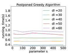
Furthermore, we investigated the influence of the parameter $n$ while keeping the other parameters constant. Fig. 6a and Fig. 6b illustrate that our algorithms consistently outperformed the original algorithms when $n\in[500,3000]$ . Additionally, the running time of each algorithm exhibited a linear increase with the growth of $n$ , which aligns with our initial expectations.

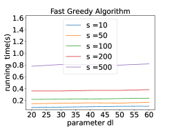
We also examined the impact of the parameter $s$ by varying its value while keeping the other parameters constant. Fig. 6a and Fig. 6b reveal that $s$ does not significantly affect the running time of the original algorithms but does impact the running time of our algorithms. Notably, our algorithms demonstrate faster performance when $s$ is smaller.

To evaluate the influence of the parameter $d$ , we varied its value while running all four algorithms. Throughout our tests, we observed that the impact of $d$ was considerably less pronounced compared to $n$ and $s$ . Consequently, we set $d$ to a sufficiently large value relative to $n$ and $s$ . As shown in Fig. 7a and Fig. 7b, indicate that $d$ does not significantly affect the running time of our algorithms, but it does have a considerable influence on the running time of the original algorithms.

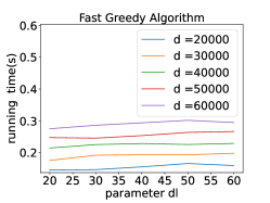
We conducted experiments to assess the influence of the parameter $\mathrm{dl}$ while keeping the other parameters constant. $\mathrm{dl}$ was selected from the interval $[1,n]$ as choosing values outside this range would render the parameter irrelevant since all nodes would remain in the market throughout the entire process. Fig. 7a and Fig. 7b show that our algorithms are faster than original algorithms when $\mathrm{dl}\in[200,600]$ .As the value of $\mathrm{dl}$ increased, the running time of all algorithms correspondingly increased. This observation highlights the impact of $\mathrm{dl}$ on the overall execution time of the algorithms.

Algorithms	$s=20$	$s=60$	$s=100$	$s=200$	$s=300$
Greedy	$706.8\pm 0.00$	$706.8\pm 0.00$	$706.8\pm 0.00$	$706.8\pm 0.00$	$706.8\pm 0.00$
FGreedy	$698.8\pm 5.07$	$704.0\pm 2.80$	$705.3\pm 2.77$	$705.8\pm 1.58$	$706.5\pm 1.31$
PGreedy	$352.5\pm 0.48$	$352.6\pm 0.47$	$352.5\pm 0.48$	$352.6\pm 0.48$	$352.6\pm 0.48$
FPGreedy	$348.1\pm 4.11$	$350.4\pm 2.00$	$351.1\pm 1.68$	$351.4\pm 1.14$	$351.5\pm 1.00$

Table 2: We use FGreedy to denote FastGreedy. We use PGreedy to denote the PostponedGreedy. We use FPGreedy to denote FastPostponedGreedy. Total weight of each algorithm,

s

is the dimension after transformation. The total weight of Greedy and PostponedGreedy don’t depend on

s

. The reason why the total weight of them isn’t the same in each case is there exists errors caused by different results of clustering the points. We test for

100

times for each algorithm in each case and calculate the mean and standard deviation of the total weight. Let

A

be the mean of the total weight of an algorithm. Let

B

be the standard deviation of the total weight of an algorithm. In each entry, we use

A\pm B

to denote the total weight of an algorithm when

s

is set by a specific value.

Table 2 shows the total weight of each algorithm when $s$ changes. Since Greedy and PostponedGreedy don’t depend on $s$ , the total weight of them doesn’t change while $s$ changes. We can see that the total weight of each optimized algorithm is very close to that of each original algorithm respectively, which means the relative error $\epsilon$ of our algorithm is very small in practice. As $s$ increases, the difference between the total weight of each optimized algorithm and each original algorithm also becomes smaller. And the total weight of FastGreedy is $2$ times of that of FastPostponedGreedy. These empirical results match our theoretical analysis. Parameter $s$ can’t affect the total weight of each algorithm. The competitive ratio of FastGreedy and FastPostponedGreedy is $\frac{1-\epsilon}{2}$ and $\frac{1-\epsilon}{4}$ respectively.

Optimal Usage of Algorithms. The results presented above demonstrate that our algorithms exhibit significantly faster performance when the values of $n$ , $d$ , and $\mathrm{dl}$ are sufficiently large. Additionally, reducing the value of $s$ leads to a decrease in the running time of our algorithms. Our proposed algorithms outperform the original algorithms, particularly when the value of $d$ is extremely large. Consequently, our algorithms are well-suited for efficiently solving problems involving a large number of nodes with substantial data entries.

More Experiments. To assess the impact of parameter $n$ in the presence of other variables, we varied the values of the remaining parameters and executed all four algorithms. As illustrated in Fig. 8, Fig. 9, Fig. 10, and Fig. 11, it is evident that the running time consistently increases with an increase in $n$ , regardless of the values assigned to the other parameters.

To investigate the impact of parameter $s$ in the presence of other variables, we varied the values of the remaining parameters and executed all four algorithms.Fig. 12 and Fig. 13 demonstrate that the value of $s$ is independent of the original algorithms. Conversely, Fig. 14 and Fig. 15 indicate that the running time of our algorithms increases with an increase in $s$ , irrespective of the values assigned to the other parameters.

To examine the impact of parameter $d$ in the presence of other variables, we varied the values of the remaining parameters and executed all four algorithms. The results depicted in Fig. 16, Fig. 17, Fig. 18 and Fig. 19 reveal that the running time of both the original and our proposed algorithms increases with an increase in $d$ , regardless of the values assigned to the other parameters.

To assess the impact of parameter $\mathrm{dl}$ in the presence of other variables, we varied the values of the remaining parameters and executed all four algorithms. As evident from Fig. 20, Fig. 21, Fig. 22, and Fig. 23, the running time consistently increases with an increase in $\mathrm{dl}$ , regardless of the values assigned to the other parameters.