Faithful and Consistent Graph Neural Network Explanations with Rationale Alignment

Graph neural networks (GNNs) are developing rapidly in recent years, with the increasing need for learning on relational data structures (Fan2019GraphNN, ; dai2022towards, ; zhao2021graphsmote, ; zhou2022graph, ; zhao2023skill, ). Generally, existing GNNs can be categorized into two categories, i.e., spectral-based approaches (bruna2013spectral, ; liang2023abslearn, ; liang2022reasoning, ) based on graph signal processing theory, and spatial-based approaches (duvenaud2015convolutional, ; atwood2016diffusion, ; xiao2021learning, ) relying upon neighborhood aggregation. Despite their differences, most GNN variants can be summarized with the message-passing framework, which is composed of pattern extraction and interaction modeling within each layer (gilmer2017neural, ). Specifically, GNNs model messages from node representations. These messages are then propagated with various message-passing mechanisms to refine node representations, which are then utilized for downstream tasks (hamilton2017inductive, ; zhang2018link, ; zhao2021graphsmote, ; zhao2022topoimb, ). Explorations are made by disentangling the propagation process (wang2020disentangled, ; zhao2022exploring, ; xiao2022decoupled, ) or utilizing external prototypes (lin2022prototypical, ; xu2022hp, ). Research has also been conducted on the expressive power (balcilar2021breaking, ; sato2020survey, ) and potential biases introduced by different kernels (nt2019revisiting, ; balcilar2021analyzing, ) for the design of more effective GNNs. Despite their success in network representation learning, GNNs are uninterpretable black box models. It is challenging to understand their behaviors even if the adopted message passing mechanism and parameters are given. Besides, unlike traditional deep neural networks where instances are identically and independently distributed, GNNs consider node features and graph topology jointly, making the interpretability problem more challenging to handle.

Recently, some efforts have been taken to interpret GNN models and provide explanations for their predictions (wang2020causal, ). Based on the granularity, existing methods can be generally grouped into two categories: (1) instance-level explanation (ying2019gnnexplainer, ), which provides explanations on the prediction for each instance by identifying important substructures; and (2) model-level explanation (baldassarre2019explainability, ; zhang2021protgnn, ), which aims to understand global decision rules captured by the target GNN. From the methodology perspective, existing methods can be categorized as (1) self-explainable GNNs (zhang2021protgnn, ; dai2021towards, ), where the GNN can simultaneously give prediction and explanations on the prediction; and (2) post-hoc explanations (ying2019gnnexplainer, ; luo2020parameterized, ; yuan2021explainability, ), which adopt another model or strategy to provide explanations of a target GNN. As post-hoc explanations are model-agnostic, i.e., can be applied for various GNNs, in this work, we focus on post-hoc instance-level explanations (ying2019gnnexplainer, ), i.e., given a trained GNN model, identifying instance-wise critical substructures for each input to explain the prediction. A comprehensive survey can be found in  (dai2022comprehensive, ).

A variety of strategies for post-hoc instance-level explanations have been explored in the literature, including utilizing signals from gradients based (pope2019explainability, ; baldassarre2019explainability, ), perturbed predictions based (ying2019gnnexplainer, ; luo2020parameterized, ; yuan2021explainability, ; shan2021reinforcement, ), and decomposition based  (baldassarre2019explainability, ; schnake2020higher, ). Among these methods, perturbed prediction-based methods are the most popular. The basic idea is to learn a perturbation mask that filters out non-important connections and identifies dominating substructures preserving the original predictions (yuan2020explainability, ). The identified important substructure is used as an explanation for the prediction. For example, GNNExplainer (ying2019gnnexplainer, ) employs two soft mask matrices on node attributes and graph structure, respectively, which are learned end-to-end under the maximizing mutual information (MMI) framework. PGExplainer (luo2020parameterized, ) extends it by incorporating a graph generator to utilize global information. It can be applied in the inductive setting and prevent the onerous task of re-learning from scratch for each to-be-explained instance. SubgraphX (yuan2021explainability, ) expects explanations to be in the form of sub-graphs instead of bag-of-edges and employs Monte Carlo Tree Search (MCTS) to find connected subgraphs that preserve predictions measured by the Shapley value. To promote faithfulness in identified explanations, some works introduced terminologies from the causality analysis domain, via estimating the individual causal effect of each edge (lin2021generative, ) or designing interventions to prevent the discovery of spurious correlations (wu2022discovering, ). Ref. (yu2020graph, ) connects the idea of identifying minimally-predictive parts in explanation with the principle of information bottleneck (tishby2015deep, ) and designs an end-to-end optimization framework for GNN explanation.

Despite the aforementioned progress in interpreting GNNs, most of these methods discover critical substructures merely upon the change of outputs given perturbed inputs. Due to this underlying inductive bias, existing label-preserving methods are heavily affected by spurious correlations caused by confounding factors in the environment. On the other hand, by aligning intermediate embeddings in GNNs, our method alleviates the effects of spurious correlations on interpreting GNNs, leading to faithful and consistent explanations.

In recent years, contrastive learning (CL) has garnered significant attention as it mitigates the need for manual annotations via unsupervised pretext tasks (LKhc2020ContrastiveRL, ; Khosla2020SupervisedCL, ; chen2020simple, ). In a typical CL framework, the model is trained in a pairwise manner, promoting attraction between positive sample pairs and repulsion between negative sample pairs (Graf2021DissectingSC, ; Wang2020UnderstandingCR, ).

Contrastive Learning (CL) techniques have recently been extended to the graph domain, constructing multiple graph views and maximizing mutual information (MI) among semantically similar instances (chen2020simple, ; feng2022adversarial, ; xia2022hypergraph, ; zhu2021empirical, ; wang2022explanation, ; liang2023knowledge, ). Existing methods primarily vary on graph augmentation techniques and contrastive pretext tasks. Graph augmentations commonly involve node-level attribute masking or perturbation (Hu2019StrategiesFP, ; Opolka2019SpatioTemporalDG, ; Velickovic2018DeepGI, ), edge dropping or rewiring (Zhu2020SelfsupervisedTO, ; You2020GraphCL, ), and graph diffusions(Hassani2020ContrastiveMR, ; Jin2021MultiScaleCS, ). Contrastive pretext tasks can be categorized into two branches, same-scale contrasts between embeddings of node (graph) pairs (Zhu2020DeepGC, ; Hassani2020ContrastiveMR, ; Zeng2022ImGCLRG, ) and cross-scale contrasts between global graph embeddings and local node representations (Velickovic2018DeepGI, ; Opolka2019SpatioTemporalDG, ). Recent works have also explored dynamic contrastive objectives (You2021GraphCL, ; Yin2021AutoGCLAG, ) via learning the augmentation strategies adaptively.

We use $\mathcal{G}=\{\mathcal{V},\mathcal{E};\mathbf{F},\mathbf{A}\}$ to denote a graph, where $\mathcal{V}=\{v_{1},\dots,v_{n}\}$ is a set of $n$ nodes and $\mathcal{E}\in\mathcal{V}\times\mathcal{V}$ is the set of edges. Nodes are accompanied by an attribute matrix $\mathbf{F}\in\mathbb{R}^{n\times d}$, and $\mathbf{F}[i,:]\in\mathbb{R}^{1\times d}$ is the $d$-dimensional node attributes of node $v_{i}$. $\mathcal{E}$ is described by an adjacency matrix $\mathbf{A}\in\mathbb{R}^{n\times n}$. ${A}_{ij}=1$ if there is an edge between node $v_{i}$ and $v_{j}$; otherwise, ${A}_{ij}=0$. For graph classification, each graph $\mathcal{G}_{i}$ has a label $Y_{i}\in\mathcal{C}$, and a GNN model $f$ is trained to map $\mathcal{G}$ to its class, i.e., $f:\{\mathbf{F},\mathbf{A}\}\mapsto\{1,2,\dots,C\}$. Similarly, for node classification, each graph $\mathcal{G}_{i}$ denotes a $K$-hop subgraph centered at node $v_{i}$ and a GNN model $f$ is trained to predict the label of $v_{i}$ based on node representation of $v_{i}$ learned from $\mathcal{G}_{i}$. The purpose of explanation is to find a subgraph $\mathcal{G}^{\prime}$, marked with binary importance mask $\mathbf{M}_{A}\in[0,1]^{n\times n}$ on adjacency matrix and $\mathbf{M}_{F}\in[0,1]^{n\times d}$ on node attributes, respectively, e.g., $\mathcal{G}^{\prime}=\{\mathbf{A}\odot\mathbf{M}_{A};\mathbf{F}\odot\mathbf{M}_{F}\}$, where $\odot$ denotes elementwise multiplication. These two masks highlight components of $\mathcal{G}$ that are important for $f$ to predict its label. With the notations, the post-hoc instance-level GNN explanation task is:

Many approaches have been designed for post-hoc instance-level GNN explanation. Due to the discreteness of edge existence and non-grid graph structures, most works apply a perturbation-based strategy to search for explanations. Generally, they can be summarized as Maximization of Mutual Information (MMI) between predicted label $\hat{Y}$ and explanation $\mathcal{G}^{\prime}$, i.e.,

where $I()$ represents mutual information and $\mathcal{P}$ denotes the perturbations on original input with importance masks $\{\mathbf{M}_{F},\mathbf{M}_{A}\}$. For example, let $\{\hat{\mathbf{A}},\hat{\mathbf{F}}\}$ represent the perturbed $\{\mathbf{A},\mathbf{F}\}$. Then, $\hat{\mathbf{A}}=\mathbf{A}\odot\mathbf{M}_{A}$ and $\hat{\mathbf{F}}=\mathbf{Z}+(\mathbf{F}-\mathbf{Z})\odot\mathbf{M}_{F}$ in GNNExplainer (ying2019gnnexplainer, ), where $\mathbf{Z}$ is sampled from marginal distribution of node attributes $\mathbf{F}$. $\mathcal{R}$ denotes regularization terms on the explanation, imposing prior knowledge into the searching process, like constraints on budgets or connectivity distributions (luo2020parameterized, ). Mutual information $I(\hat{Y},\mathcal{G}^{\prime})$ quantifies consistency between original predictions $\hat{Y}=f(\mathcal{G})$ and prediction of candidate explanation $f(\mathcal{G}^{\prime})$, which promotes the positiveness of found explanation $\mathcal{G}^{\prime}$. Since mutual information measures the predictive power of $\mathcal{G}^{\prime}$ on $Y$, this framework essentially tries to find a subgraph that can best predict the original output $\hat{Y}$. During training, a relaxed version (ying2019gnnexplainer, ) is often adopted as:

where $H_{C}$ denotes cross-entropy. With this same objective, existing methods mainly differ from each other in optimization and searching strategies.

Different aspects regarding the quality of explanations can be evaluated (nauta2022anecdotal, ). Among them, two most important criteria are faithfulness and consistency. Faithfulness measures the descriptive accuracy of explanations, indicating how truthful they are compared to behaviors of the target model. Consistency considers explanation invariance, which checks that identical input should have identical explanations. However, as shown in Figure 1, the existing MMI-based framework is sub-optimal in terms of these criteria. The cause of this problem is rooted in its learning objective, which uses prediction alone as guidance in search of explanations. Due to the complex graph structure, the prediction alone as a guide could result in spurious explanations. A detailed analysis will be provided in the next section.

Instance-level post-hoc explanation dedicates to finding discriminative substructures that the target model $f$ depends upon. The traditional objective in Equation 2 can identify minimal predictive parts of input, however, it is dangerous to directly take them as explanations. Due to diversity in graph topology and combinatory nature of sub-graphs, multiple distinct substructures could be identified leading to the same prediction, as discussed in Section 3.

For an explanation substructure $\mathcal{G}^{\prime}$ to be faithful, it should follow the same rationale as the original graph $\mathcal{G}$ inside the internal inference of to-be-explained model $f$. To achieve this goal, the explanation $\mathcal{G}^{\prime}$ should be aligned to $\mathcal{G}$ w.r.t the decision mechanism, reflected in Figure 2(a). However, it is non-trivial to extract and compare the critical causal variables $C$ and confounding variables $S$ due to the black box nature of the target GNN model to be explained.

Following the causal analysis in Section 3, we propose to take an alternative approach by looking into internal embeddings learned by $f$. Causal variables $C$ are encoded in representation space extracted by $f$, and out-of-distribution effects can also be reflected by analyzing embedding distributions. An assumption can be safely made: if two graphs are mapped to embeddings near each other by a GNN layer, then these graphs are seen as similar by it and would be processed similarly by following layers. With this assumption, a proxy task can be designed by aligning internal graph embeddings between $\mathcal{G}^{\prime}$ and $\mathcal{G}$. This new task can be incorporated into Framework 1 as an auxiliary optimization objective.

Let $\mathbf{h}_{v}^{l}$ be the representation of node $v$ at the $l$-th GNN layer with $\mathbf{h}_{v}^{0}=\mathbf{F}[v,:]$. Generally, the inference process inside GNN layers can be summarized as a message-passing framework:

where $\text{Message}_{l}$ and $\text{Update}_{l}$ are the message function and update function at $l$-th layer, respectively. $\mathcal{N}(v)$ is the set of node $v$’s neighbors. Without loss of generality, the graph pooling layer can also be presented as:

where ${P}_{v,v^{\prime}}$ denotes mapping weight from node $v$ in layer $l$ to node $v^{\prime}$ in layer $l+1$ inside the myriad of GNN for graph classification. We propose to align embedding $\mathbf{h}_{v}^{l+1}$ at each layer, which contains both node and local neighborhood information.

Achieving alignment in the embedding space is not straightforward. It has several distinct difficulties. (1) It is difficult to evaluate the distance between $\mathcal{G}$ and $\mathcal{G}^{\prime}$ in this embedding space. Different dimensions could encode different features and carry different importance. Furthermore, $\mathcal{G}^{\prime}$ is a substructure of the original $\mathcal{G}$, and a shift on unimportant dimensions would naturally exist. (2) Due to the complexity of graph/node distributions, it is non-trivial to design a measurement of alignments that is both computation-friendly and can correlate well to distance on the distribution manifold.

To address these challenges, we design a strategy to identify explanatory substructures and preserve their alignment with original graphs in a distribution-aware manner. The basic idea is to utilize other graphs to obtain a global view of the distribution density of embeddings, providing a better measurement of alignment. Concretely, we obtain representative node/graph embeddings as anchors and use distances to these anchors as the distribution-wise representation of graphs. Alignment is conducted on obtained representation of graph pairs. Next, we go into details of this strategy.

• •

  First, using graphs $\{\mathcal{G}_{i}\}_{i=1}^{m}$ from the same dataset, a set of node embeddings can be obtained as $\{\{\mathbf{h}^{l}_{v,i}\}_{v\in\mathcal{V}^{\prime}_{i}}\}_{i=1}^{m}$ for each layer $l$, where $\mathbf{h}_{v,i}$ denotes embedding of node $v$ in graph $\mathcal{G}_{i}$. For node-level tasks, we set $\mathcal{V}^{\prime}_{i}$ to contain only the center node of graph $\mathcal{G}_{i}$. For graph-level tasks, $\mathcal{V}^{\prime}_{i}$ contains nodes set after graph pooling layer, and we process them following $\{\sum_{v\in\mathcal{V}^{\prime}_{i}}\mathbf{h}^{l+1}_{v,i}/|\mathcal{V}^{\prime}_{i}|\}_{i=1}^{m}$ to get global graph representation.

• •

  Then, a clustering algorithm is applied to the obtained embedding set to get $K$ groups. Clustering centers of these groups are set to be anchors, annotated as $\{\mathbf{h}^{l+1,k}\}_{k=1}^{K}$. In experiments, we select DBSCAN (ester1996density, ) as the clustering algorithm, and tune its hyper-parameters to get around $20$ groups.

• •

  At $l$-th layer, $\mathbf{h}_{v}^{l+1}$ is represented in terms of relative distances to those $K$ anchors, as $\mathbf{s}_{v}^{l}\in\mathbb{R}^{1\times K}$ with the $k$-th element calculated as $\mathbf{s}_{v}^{l+1,k}=\|\mathbf{h}^{l+1}_{v}-\mathbf{h}^{l+1,k}_{v}\|_{2}$.

Alignment between $\mathcal{G}^{\prime}$ and $\mathcal{G}$ can be achieved by comparing their representations at each layer. The alignment loss is computed as:

This metric provides a lightweight strategy for evaluating alignments in the embedding distribution manifold, by comparing relative positions w.r.t representative clustering centers. This strategy can naturally encode the varying importance of each dimension. Fig. 2(b) gives an example, where $\mathcal{G}$ is the graph to be explained and the red stars are anchors. $\mathcal{G}^{\prime}_{1}$ and $\mathcal{G}^{\prime}_{2}$ are both similar to $\mathcal{G}$ w.r.t absolute distances; while it is easy to see $\mathcal{G}^{\prime}_{1}$ is more similar to $\mathcal{G}$ w.r.t to the anchors. In other words, the anchors can better measure the alignment to filter out spurious explanations.

This alignment loss is used as an auxiliary task incorporated into MMI-based framework in Equation 2 to get faithful explanation as:

where $\lambda$ controls the balance between prediction preservation and embedding alignment. $\mathcal{L}_{Align}$ is flexible to be incorporated into various existing explanation methods.

As a simpler and more direct implementation, we also design a variant based on absolute distance. For layers without graph pooling, the objective can be written as $\sum_{l}\sum_{v\in\mathcal{V}}\|\mathbf{h}_{v}^{l}-{\mathbf{h}}_{v}^{{}^{\prime}l}\|_{2}^{2}$. For layers with graph pooling, as the structure could be different, we conduct alignment on global representation $\sum_{v\in\mathcal{V}^{\prime}}\mathbf{h}^{l+1}_{v}/|\mathcal{V}^{\prime}|$, where $\mathcal{V}^{\prime}$ denotes node set after pooling.

In this strategy, we model the latent embeddings of nodes (or graphs) using a mixture of Gaussian distributions, with representative node/graph embeddings as anchors (Gaussian centers). The produced embedding of each input can be compared with those prototypical anchors, and the semantic information of inputs taken by the target model would be encoded by relative distances from them.

Concretely, we first obtain prototypical representations, annotated as $\{\mathbf{h}^{l,k}\}_{k=1}^{K}$, by running the clustering algorithm on collected embeddings $\{\{\mathbf{h}^{l}_{v,i}\}_{v\in\mathcal{V}^{\prime}_{i}}\}_{i=1}^{m}$ from graphs $\{\mathcal{G}_{i}\}_{i=1}^{m}$, in the same strategy as introduced in Sec. 4.2. Clutering algorithm DBSCAN (ester1996density, ) is adopted and we tune its hyper-parameters to get around $20$ groups.

Next, the probability of encoded representation ${\mathbf{h}}^{l}$ falling into each prototypical Gaussian centers $\{\mathbf{h}^{l,k}\}_{k=1}^{K}$ can be computed as:

This distribution probability can serve as a natural tool for depicting the semantics of the input graph learned by the GNN model. Consequently, the distance between ${\mathbf{h}}_{v}^{{}^{\prime}l}$ and $\mathbf{h}_{v}^{l}$ can be directly measured as the KL-divergence w.r.t this distribution probability:

where $\mathbf{p}_{v}^{{}^{\prime}l}\in\mathbb{R}^{K}$ denotes the distribution probability of candidate explanation embedding, $\mathbf{h}_{v}^{{}^{\prime}l}$. Using this strategy, the alignment loss between original graph and the candidate explanation is computed as:

which can be incorporated into the revised explanation framework proposed in Eq. 6.

Comparison Compared with the alignment loss based on relative distances against anchors in Eq. 5, this new objective offers a better strategy in taking distribution into consideration. Specifically, we can show the following two advantages:

• •

  In obtaining the distribution-aware representation of each instance, this variant uses a Gaussian distance kernel (Eq. 7) while the other one uses Euclidean distance in Sec. 4.2, which may amplify the influence of distant anchors. We can prove this by examining the gradient of changes in representation w.r.t GNN embeddings $\mathbf{h}_{v}$. In the $l$-th layer at dimension $k$, the gradient of the previous variant can be computed as:

  (10)

  $$\frac{\partial s_{v}^{l,k}}{\partial\mathbf{h}_{v}^{l}}=2\cdot(\mathbf{h}_{v}^{l}-\mathbf{h}_{v}^{l,k})$$

  On the other hand, the gradient of this variant is:

  (11)

  $\displaystyle\frac{\partial p_{v}^{l,k}}{\partial\mathbf{h}_{v}^{l}}$

  $\displaystyle\approx-\frac{\exp(-\|{\mathbf{h}}_{v}^{l}-\mathbf{h}^{l,k}\|_{2}^{2}/2\sigma^{2})\cdot(\mathbf{h}_{v}^{l}-\mathbf{h}_{v}^{l,k})}{\sigma^{2}\cdot\sum_{j=1}^{K}\exp(-\|{\mathbf{h}}_{v}^{l}-\mathbf{h}^{l,k}\|_{2}^{2}/2\sigma^{2})}$

  It is easy to see that for the previous variant, the magnitude of gradient would grow linearly w.r.t distances towards corresponding anchors. For this variant, on the other hand, the term $\frac{\exp(-\|{\mathbf{h}}_{v}^{l}-\mathbf{h}^{l,k}\|_{2}^{2}/2\sigma^{2})}{\sigma^{2}\cdot\sum_{j=1}^{K}\exp(-\|{\mathbf{h}}_{v}^{l}-\mathbf{h}^{l,k}\|_{2}^{2}/2\sigma^{2})}$ would down-weight the importance of those distant anchors while up-weight the importance of similar anchors, which is more desired in obtaining distribution-aware representations.

• •

  In computing the distance between representations of two inputs, this variant adopts the KL divergence as in Eq. 8, which would be scale-agnostic compared to the other one directly using Euclidean distance as in Eq. 5. Again, we can show the gradient of alignment loss towards obtained embeddings that encode distribution information. It can be observed that for the previous variant:

  (12)

  $$\frac{\partial d(\mathbf{s}_{v}^{l},\mathbf{s}_{v}^{{}^{\prime}l})}{\partial s_{v}^{{}^{\prime}l,k}}=2\cdot(s_{v}^{l,k}-s_{v}^{{}^{\prime}l,k})$$

  For this variant based on Gaussian mixture model, the gradient can be computed as:

  (13)

  $$\frac{\partial d(\mathbf{p}_{v}^{l},\mathbf{p}_{v}^{{}^{\prime}l})}{\partial p_{v}^{{}^{\prime}l,k}}=1+\log(\frac{{p}_{v}^{{}^{\prime}l,k}}{{p}_{v}^{l,k}})$$

  It can be observed that the previous strategy focuses on representation dimensions with a large absolute difference, while would be sensitive towards the scale of each dimension. On the other hand, this strategy uses the summation between the logarithm of relative difference with a constant, which is scale-agnostic towards each dimension.

In this strategy, we further consider the utilization of deep models to capture the distribution and estimate the semantic similarity of two inputs, and incorporate it into the alignment loss for discovering faithful and consistent explanations. Specifically, we train a deep model to estimate the mutual information (MI) between two input graphs, and use its prediction as a measurement of alignment between original graph and its candidate explanation. This strategy circumvents the reliance on heuristic strategies and is purely data-driven, which can be learned in an end-to-end manner.

To learn the mutual information estimator, we adopt a neural network and train it to be a Jensen-Shannon MI estimator (hjelm2018learning, ). Concretely, we train this JSD-based estimator on top of intermediate embeddings with the learning objective as follows, which offers better stability in optimization:

where $\mathbb{E}$ denotes expectation. In this equation, $T^{l}(\cdot)$ is a compatibility estimation function in the $l$-th layer, and we denote $\{T^{l}(\cdot)\}_{l}$ as the MI estimator $g_{mi}$. Activation function $sp(\cdot)$ is the softplus function, and $\mathbf{h}_{v}^{+}$ represents the embedding of augmented node $v$ that is a positive pair of $v$ in the original graph. On the contrary, $\mathbf{h}_{v}^{-}$ denotes the embedding of augmented node $v$ that is a negative pair of original input. A positive pair is obtained through randomly dropping intermediate neurons, corresponding to masking out a ratio of original input, and a negative pair is obtained as embeddings of different nodes. This objective can guide $g_{mi}$ to capture the correlation or similarity between two input graphs encoded by the target model. Note that to further improve the learning of MI estimator, more advanced graph augmentation techniques can be incorporated for obtaining positive/negative pairs, following recent progresses in graph contrastive learning (feng2022adversarial, ; xia2022hypergraph, ). In this work, we stick to the strategy adopted in  (hjelm2018learning, ) for its popularity, and leave that for future explorations. With this MI estimator learned, alignment loss between $\mathcal{G}$ and $\mathcal{G}^{{}^{\prime}}$ can be readily computed:

which can be incorporated into the revised explanation framework proposed in Eq. 6.

In this strategy, we design a data-driven approach by capturing the mutual information between two inputs, which circumvents the potential biases of using human-crafted heuristics.

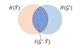
From previous discussions, it is shown that $\mathcal{G}^{\prime}$ obtained via Equation 1 cannot be safely used as explanations. One main drawback of existing GNN explanation methods lies in the inductive bias that the same outcomes do not guarantee the same causes, leaving existing approaches vulnerable towards spurious explanations. An illustration is given in Figure 3. Objective proposed in Equation 1 optimizes the mutual information between explanation candidate $\mathcal{G}^{\prime}$ and $\hat{Y}$, corresponding to maximize the overlapping between $H(\mathcal{G}^{\prime})$ and $H(\hat{Y})$ in Figure 3(a), or region $S_{1}\cup S_{2}$ in Figure 3(b). Here, $H$ denotes information entropy. However, this learning target cannot prevent the danger of generating spurious explanations. Provided $\mathcal{G}^{\prime}$ may fall into the region $S_{2}$, which cannot faithfully represent graph $\mathcal{G}$. Instead, a more sensible objective should be maximizing region $S_{1}$ in Figure 3(b). The intuition behind this is that in the search input space that causes the same outcome, identified $\mathcal{G}^{\prime}$ should account for both representative and discriminative parts of original $\mathcal{G}$, to prevent spurious explanations that produce the same outcomes due to different causes. Concretely, finding $\mathcal{G}^{\prime}$ that maximize $S_{1}$ can be formalized as:

$I(\mathcal{G},\mathcal{G^{\prime}},\hat{Y})$ is intractable as the latent generation mechanism of $\mathcal{G}$ is unknown. In this part, we expand this objective, connect it to Equation 6, and construct its proxy optimizable form as:

Since both $H(\mathcal{G}^{\prime}|\mathcal{G},\hat{Y})$ and $H(\mathcal{G}^{\prime})$ depicts entropy of explanation $\mathcal{G}^{\prime}$ and are closely related to perturbation budgets, we can neglect these two terms and get a surrogate optimization objective for $\max_{\mathcal{G}^{\prime}}I(\mathcal{G},\mathcal{G^{\prime}},\hat{Y})$ as $\max_{\mathcal{G}^{\prime}}I(\hat{Y},\mathcal{G^{\prime}})+I(\mathcal{G}^{\prime},\mathcal{G})$.

In $\max_{\mathcal{G}^{\prime}}I(\hat{Y},\mathcal{G^{\prime}})+I(\mathcal{G}^{\prime},\mathcal{G})$, the first term $\max_{\mathcal{G}^{\prime}}I(\hat{Y},\mathcal{G^{\prime}})$ is the same as Eq.(1). Following  (ying2019gnnexplainer, ), We relax it as $\min_{\mathcal{G}^{\prime}}H_{C}(\hat{Y},\hat{Y}^{\prime}|\mathcal{G^{\prime}})$, optimizing $\mathcal{G}^{\prime}$ to preserve original prediction outputs. The second term, $\max_{\mathcal{G}^{\prime}}I(\mathcal{G}^{\prime},\mathcal{G})$, corresponds to maximizing consistency between $\mathcal{G}^{\prime}$ and $\mathcal{G}$. Although the graph generation process is latent, with the safe assumption that embedding $\mathbf{E}_{\mathcal{G}}$ extracted by $f$ is representative of $\mathcal{G}$, we can construct a proxy objective $\max_{\mathcal{G}^{\prime}}I(\mathbf{E}_{\mathcal{G}^{\prime}},\mathbf{E}_{\mathcal{G}})$, improving the consistency in the embedding space. In this work, we optimize this objective by aligning their representations, either optimizing a simplified distance metric or conducting distribution-aware alignment.

To answer RQ1, we compare explanation methods in terms of AUROC score and explanation fidelity.

One problem of spurious explanation is that, due to the randomness in initialization of the explainer, the explanation for the same instance given by a GNN explainer could be different for different runs, which violates the consistency of explanations. To test the severity of this problem and answer RQ2, we evaluate the proposed framework in terms of explanation consistency. We adopt GNNExplainer and PGExplainer as baselines. Specifically, SHD distance among explanatory edges with top-$k$ importance weights identified each time is computed. Then, the results are averaged for all instances in the test set. Each experiment is conducted $5$ times, and the average consistency on dataset Tree-Grid and Mutag are reported in Table 3 and Table 4, respectively. Larger distances indicate inconsistent explanations. From the table, we can observe that existing method following Equation 1 suffers from the consistency problem. For example, average SHD distance on top-$6$ edges is $4.39$ for GNNExplainer. Introducing the auxiliary task of aligning embeddings can significantly improve explainers in terms of this criterion. Of these different alignment strategies, the variant based on Gaussian mixture model shows the strongest performance in most cases. After incorporating Align_Gaus on dataset TreeGrid, SHD distance of top-$6$ edges drops from $4.39$ to $2.13$ for GNNExplainer and from $1.38$ to $0.13$ for PGExplainer. After incorporating it on dataset Mutag, SHD distance of top-$6$ edges drops from $4.78$ to $3.85$ for GNNExplainer and from $3.42$ to $1.15$ for PGExplainer. These results validate the effectiveness of our proposal in obtaining consistent explanations.

Existing graph explanation benchmarks are usually designed to be less ambiguous, containing only one oracle cause of labels, and identified explanatory substructures are evaluated via comparing with the ground-truth explanation. However, this result could be misleading, as faithfulness of explanation in more complex scenarios is left untested. Real-world datasets are usually rich in spurious patterns and a trained GNN could contain diverse biases, setting a tighter requirement on explanation methods. Thus, to evaluate if our framework can alleviate the spurious explanation issue and answer RQ3, we create a new graph-classification dataset: MixMotif, which enables us to train a biased GNN model, and test whether explanation methods can successfully expose this bias.

Specifically, inspired by  (wu2022discovering, ), we design three types of base graphs, i.e., Tree, Ladder, and Wheel, and three types of motifs, i.e., Cycle, House, and Grid. With a mix ratio $\gamma$, motifs are preferably attached to base graphs. For example, Cycle is attached to Tree with probability $\frac{2}{3}\gamma+\frac{1}{3}$, and to others with probability $\frac{1-\gamma}{3}$. So are the cases for House to Ladder and Grid to Wheel. Labels of obtained graphs are set as type of the motif. When $\gamma$ is set to $0$, each motif has the same probability of being attached to the three base graphs. In other words, there’s no bias on which type of base graph to attach for each type of motif. Thus, we consider the dataset with $\gamma=0$ as clean or bias-free. We would expect GNN trained on data with $\gamma=0$ to focus on the motif structure for motif classification. However, when $\gamma$ becomes larger, the spurious correlation between base graph and the label would exist, i.e., a GNN might utilize the base graph structure for motif classification instead of relying on the motif structure. For each setting, the created dataset contains $3,000$ graphs, and train:evaluation:test are split as $5:2:3$.

In this experiment, we set $\gamma$ to $0$ and $0.7$ separately, and train GNN $f_{0}$ and $f_{0.7}$ for each setting. Two models are tested in graph classification performance. Then, explanation methods are applied to and fine-tuned on $f_{0}$. Following that, these explanation methods are applied to explain $f_{0.7}$ using found hyper-parameters. Results are summarized in Table 5.

From Table 5, we can observe that (1) $f_{0}$ achieves almost perfect graph classification performance during testing. This high accuracy indicates that it captures the genuine pattern, relying on motifs to make predictions. Looking at explanation results, it is shown that our proposal offers more faithful explanations, achieving higher AUROC on motifs. (2) $f_{0.7}$ fails to predict well with $\gamma=0$, showing that there are biases in it and it no longer depends solely on the motif structure for prediction. Although ground-truth explanations are unknown in this case, a successful explanation should expose this bias. However, PGExplainer would produce similar explanations as the clean model, still highly in accord with motif structures. Instead, for explanations produced by embedding alignment, AUROC score would drop from $0.795$ to $0.266$, exposing the change in prediction rationales, hence able to expose biases. (3) In summary, our proposal can provide more faithful explanations for both clean and mixed settings, while PGExplainer would suffer from spurious explanations and fail to faithfully explain GNN’s predictions, especially in the existence of biases.

In this part, we vary the hyper-parameter $\lambda$ to test the sensitivity of the proposed framework toward its values. $\lambda$ controls the weight of our proposed embedding alignment task. To keep simplicity, all other configurations are kept unchanged, and $\lambda$ is varied within the scale $[1e-3,1e-2,1e-1,1,10,1e2,1e3\}$. PGExplainer is adopted as the base method. Experiments are randomly conducted $3$ times on dataset Tree-Grid and Mutag. Averaged results are visualized in Figure 5. From the figure, we can make the following observations:

• •

  For all four variants, increasing $\lambda$ has a positive effect at first, and the further increase would result in a performance drop. For example on the Tree-Grid dataset, best results of variants based on anchors, latent Gaussian mixture models and mutual information scores are all obtained with $\lambda$ around $1$. When $\lambda$ is small, the explanation alignment regularization in Eq. 6 will be underweighted. On the other hand, a too-large $\lambda$ may underweight the MMI-based explanation framework, which preserves the predictive power of obtained explanations.

• •

  Among these variants, the strategy based on latent Gaussian mixture models shows the strongest performance in most cases. For example, for both datasets Tree-Grid and Mutag, this variant achieves the highest AUROC scores on identified explanatory edges. On the other hand, the variant directly using Euclidean distances shows inferior performances in most cases. We attribute this to their different ability in modeling the distribution and conducting alignment.