Faithful and Accurate Self-Attention Attribution for Message Passing Neural Networks via the Computation Tree Viewpoint

Yong-Min Shin¹, Siqing Li², Xin Cao², Won-Yong Shin¹ Corresponding Author.

Abstract

The self-attention mechanism has been adopted in various popular message passing neural networks (MPNNs), enabling the model to adaptively control the amount of information that flows along the edges of the underlying graph. Such attention-based MPNNs (Att-GNNs) have also been used as a baseline for multiple studies on explainable AI (XAI) since attention has steadily been seen as natural model interpretations, while being a viewpoint that has already been popularized in other domains (e.g., natural language processing and computer vision). However, existing studies often use naïve calculations to derive attribution scores from attention, undermining the potential of attention as interpretations for Att-GNNs. In our study, we aim to fill the gap between the widespread usage of Att-GNNs and their potential explainability via attention. To this end, we propose GAtt, edge attribution calculation method for self-attention MPNNs based on the computation tree, a rooted tree that reflects the computation process of the underlying model. Despite its simplicity, we empirically demonstrate the effectiveness of GAtt in three aspects of model explanation: faithfulness, explanation accuracy, and case studies by using both synthetic and real-world benchmark datasets. In all cases, the results demonstrate that GAtt greatly improves edge attribution scores, especially compared to the previous naïve approach. Our code is available at https://github.com/jordan7186/GAtt.

1 Introduction

Background & motivation.

In graph learning, graph neural networks (GNNs) (Wu et al. 2021) have been used as the de facto architecture, since they can effectively encode the graph structure along with node (or edge) features. Among various GNNs, several models have successfully incorporated the self-attention mechanism (Vaswani et al. 2017) into message passing neural networks (MPNNs) (Gilmer et al. 2017; Bronstein et al. 2021). Such (self-)attention-based MPNNs (dubbed Att-GNNs) have been one of the staple GNN architectures, and the self-attention mechanism of Att-GNNs themselves has been extensively analyzed in the literature (Knyazev, Taylor, and Amer 2019; Lee et al. 2019; Sun et al. 2023).¹¹1As such, we refer to the term ‘GNN’ as MPNN-style architectures unless explicitly stated otherwise. Furthermore, several studies have focused solely on analyzing GAT (Velickovic et al. 2018), the most representative Att-GNN model (Mustafa, Bojchevski, and Burkholz 2023; Fountoulakis et al. 2023).

Similarly as in other neural network models, GNNs are regarded as black-box models that lack interpretability, which has led to numerous studies developing explanation methods for GNNs (Li et al. 2022; Yuan et al. 2023). While such explanation methods have been widely developed, attention has also been frequently considered as a fundamental tool for GNN explanations (Ying et al. 2019; Luo et al. 2020; Sánchez-Lengeling et al. 2020). The choice of attention as a baseline is natural, as self-attention itself can be viewed as a direct way to provide model interpretations without any separate explanation method (Lee, Shin, and Kim 2017; Ghaeini, Fern, and Tadepalli 2018; Hao et al. 2021; Aflalo et al. 2022; Deiseroth et al. 2023). This viewpoint has already been extensively investigated in transformers, the most representative architecture with attention (Bahdanau, Cho, and Bengio 2015; Xu et al. 2015; Vig 2019; Dosovitskiy et al. 2021; Caron et al. 2021). There is even a significant body of research debating the validity of self-attention as explanations in natural language processing (NLP) (Jain and Wallace 2019; Wiegreffe and Pinter 2019; Bibal et al. 2022). However, there has been no such in-depth discussion from the domain of GNN explanations, mostly employing the layer-wise average of attention weights retrieved from a GAT model as explanations at best.

We argue that such naïve usage of attention for interpretations largely undermines the potential of Att-GNNs as an explainable model. In the case of transformers, a number of advanced attribution methods using attention have been proposed to calculate token attributions, and have been empirically proven that attention can be effectively used to decipher the underlying model (Abnar and Zuidema 2020; Chefer, Gur, and Wolf 2021a, b; Hao et al. 2021). Analogous to transformers, our study aims to formulate a post-processing method for the attention weights in Att-GNNs that is able to extract high-quality edge attributions (i.e., to assign contributions of edges to the model) and capture the behavior of Att-GNNs more precisely. To the best of our knowledge, we are the first to address this issue within the scope of general Att-GNNs, thus filling in the literature of explanations via attention (see the red part of Table 1).

Table 1: Overview of prior works on using attention as explanations. Despite various methods being developed for calculating token attributions for transformers, no corresponding method has yet been developed for calculating edge attributions for Att-GNNs.

Model	Naïve methods	Advanced methods
Transformers		(Abnar and Zuidema 2020)
	Raw attention	(Chefer, Gur, and Wolf 2021a)
	(Vig 2019)	(Chefer, Gur, and Wolf 2021b)
		(Hao et al. 2021) etc.
	Layer-wise averaging
Att-GNNs	(Ying et al. 2019)	This work (GAtt)
	(Luo et al. 2020)

Main contributions.

In this study, we address the problem of developing an effective edge attribution method using attention weights in Att-GNNs. Our key insight is that edge attributions with attention can be advanced by aligning with the feed-forward process of MPNNs, i.e., thinking in terms of the computation tree viewpoint, a rooted subtree that shows the local computation structure around a target node (see the middle part of Figure 1). Based on observing the computation tree, we assert that the edge attribution function should encompass two crucial principles: P1) proximity to the target node and P2) its position in the computation tree, thus aligning with the feed-forward process.

To this end, we introduce GAtt, a simple yet effective solution to the edge attribution problem by integrating the computation tree of a given target node. Specifically, GAtt adds attention weights in the underlying Att-GNN across the computation tree while adjusting their influence by employing targeted multiplication factors for attention weights guiding towards the target node. As an example, Figure 1 visualizes edge attribution scores from different edge attribution calculation methods using the same model. The attribution scores from GAtt (see the right red box in Figure 1) show that the model places high emphasis on the correct infection path (highlighted as blue nodes). Such conclusion could not have been reached if we were to use simple layer-wise averaging (see the left box in Figure 1) as the tool for interpretations. To prove the effectiveness of GAtt, we run extensive experiments by answering pivotal facets of interpretations—faithfulness and explanation accuracy—of Att-GNNs across diverse real-world and synthetic datasets. Despite the simplicity of GAtt, empirical results demonstrate that the application of GAtt to process attention weights within the underlying model produces substantively improved explanation capabilities, excelling in both faithfulness and explanation accuracy. We also perform an ablation study in which we introduce two variants of GAtt, namely GAtt ${}_{\textsc{sim}}$ and GAtt ${}_{\textsc{avg}}$ , each of which corresponds to a removal of one critical design element (i.e., P1 or P2) of our method. Our analysis reveals clear deterioration of the quality of the edge attributions in all measures for both variants, which justifies the necessity of our two design elements. Finally, we remark that GAtt is a straightforward calculation module (i.e., does not involve any optimization/learning process), therefore brings the benefit of being hyperparameter-free and deterministic. In summary, we conclude that Att-GNNs are indeed highly explainable when adopting the proper interpretation, i.e., adjustment of attention weights by taking the viewpoint of the computation tree. Note that graph transformers (Ying et al. 2021; Kreuzer et al. 2021; Chen et al. 2023) are beyond the scope of this study since transformers have already been analyzed and advanced by numerous studies (see Table 1). Our contributions are summarized as follows:

Refer to caption — Figure 1: An visualization of our method (GAtt, right) against the previous approach (AvgAtt, left) on the Infection dataset, where the correct infection path is highlighted as the blue nodes.

◼

Key observations: We make key observations and design principles that are crucial in edge attribution calculation by integrating the computation tree of the target node during its feed-forward process.
◼

Novel methodology: We propose GAtt, a new method to calculate edge attributions from attention weights in Att-GNNs by integrating the computation tree of the given GNN model.
◼

Extensive evaluations: We extensively demonstrate that Att-GNNs are shown to be more faithful and accurate when using our proposed method compared to the simple alternative.

It should be noted that as long as Att-GNN architectures are employed, GAtt is model-agnostic and standalone without any learning modules. We refer to Appendix A for a comprehensive review of related studies.

2 Edge Attribution Calculation in Att-GNNs

In this section, we first describe the notation used in the paper. Then, we formalize the problem of calculating edge attributions in Att-GNNs, and propose GAtt, an approach to incorporate the computation tree into edge attributions.

2.1 Notations

Let us denote a given undirected graph as a tuple $G=(\mathcal{V},\mathcal{E})$ , where $\mathcal{V}$ is the set of nodes and $\mathcal{E}$ is the set of edges. We denote the edge connecting two nodes $v_{i},v_{j}\in\mathcal{V}$ as $e_{ij}\in\mathcal{E}$ . We consider undirected graphs, i.e., $e_{j,i}\in\mathcal{E}$ if $e_{i,j}\in\mathcal{E}$ . The set of neighbors of node $v_{i}$ is denoted as $\mathcal{N}_{i}$ .

2.2 Problem Statement

We are given a graph $G=(\mathcal{V},\mathcal{E})$ , the Att-GNN model $f$ with $L$ layers, and a target node $v_{i}\in\mathcal{V}$ of interest. The attention weights calculated from $f$ are denoted as $\mathcal{A}=\{{\bf A}(l)\}_{l=1}^{L}$ , where ${\bf A}(l)\in\mathbb{R}^{|\mathcal{V}|\times|\mathcal{V}|}$ and $[{\bf A}(l)]_{j,i}=\alpha_{i,j}^{l}$ is the attention weight of edge $e_{i,j}$ in the $l$ -th layer (with $l=1$ being the input layer). The problem of edge attribution calculation is characterized by an edge attribution function $\Phi(v,\mathcal{A},e_{i,j})\triangleq\phi_{i,j}^{v}$ such that the edge attribution score $\phi_{i,j}^{v}$ accounts for the contribution of edge $e_{i,j}$ to the underlying model’s calculation for node $v$ (i.e., faithfulness to $f$ ).

In our study, our objective is to design $\Phi$ using the computation tree in Att-GNNs alongside several observations and key design principles, which will be specified later. To design such a function $\Phi$ , we argue that the computation tree of Att-GNNs should be considered for the precise calculation of $\phi_{i,j}^{v}$ , incorporating its several key properties. Note that, although most post hoc instance-level explanation methods for GNNs (Ying et al. 2019; Luo et al. 2020) also have a similar objective in terms of calculating $\phi_{i,j}^{v}$ , they do not take advantage of attention weights $\mathcal{A}$ . Additionally, although we mainly consider node-level tasks throughout the paper as a representative task, we also demonstrate that the idea of GAtt can also be extended for graph-level tasks (see Appendix E.5).

2.3 From Attention to Attribution

We first visualize the computation tree in a Att-GNN, which will lead to several important observations to guide GAtt, an edge attribution calculation method given the attention weights in the Att-GNN model.

Visualizing the Computation Tree.

To provide an illustrative example, we train a 2-layer GAT model (Velickovic et al. 2018) with a single attention head on the synthetic infection benchmark dataset (Faber, Moghaddam, and Wattenhofer 2021). Figure 2(a) shows the 2-hop subgraph from target node 27, which contains all nodes and edges that the model involves from node 27’s point of view. The computation tree in the GAT is commonly expressed as a rooted subtree (Sato, Yamada, and Kashima 2021), as shown in Figure 2(b) for node 27. In the figure, the information flows from leaf nodes at depth 2 to the root node 27 at depth 0, which exhibits an apparently different structure from that of the subgraph in Figure 2(a). Note that the attention weights are calculated in each graph attention layer for each edge in $\mathcal{E}$ .

Design Principles.

We begin by making several observations from the computation tree:

(O1)

Identical edges can appear multiple times in the computation tree. For example, edge $e_{40,27}$ in Figure 2(a) appears twice in Figure 2(b).
(O2)

Nodes do not appear uniformly in the computation tree. Specifically, nodes that are $k$ -hops away from the target node do not exist in depth $k^{\prime}$ for $0<k^{\prime}<k$ (e.g., node 70 appears only at depth 2 while node 40 appears three times).
(O3)

The graph attention layer always includes self-loops during its feed-forward process.

Based on the above observations, we would like to state two design principles that are desirable when designing the edge attribution function $\Phi$ .

(P1)

Proximity effect: Edges within closer proximity to the target node tend to highly impact the model’s prediction compared with distant edges, since they are likely to appear more frequently in the computation tree.
(P2)

Contribution adjustment: The contribution of an edge in the computation tree should be adjusted by its position (i.e., other edges in the path towards the root).

By these standards, we revisit Figure 2(b). We first see that edges close to the target node such as $e_{40,27}$ appear twice, whereas distant edges such as $e_{70,40}$ appear only once (P1). Moreover, we empirically show that this principle (P1) holds in most real-world datasets (refer to Appendix E.6). Additionally, for the attention weights from the last graph attention layer (i.e., edges connecting nodes at depth 1 to the root node), each edge tends to have roughly the value of $0.25$ for the attention weights. In consequence, the information flowing from the first graph attention layer (i.e., edges connecting leaf nodes to nodes at depth 1) will be diminished by roughly $0.25$ as it reaches the root node (P2).

Proposed Method.

To design the edge attribution function $\Phi$ , we start by formally defining the computation tree alongside the flow and the attention flow.

Definition 2.1 (Computation tree).

The computation tree for an $L$ -layer Att-GNN in our study is defined as a rooted subtree of height $L$ with the target node as the root node. For each node in the tree at depth $d$ , the neighboring nodes and itself are at depth $d+1$ with edges directed towards node $v$ .

According to Definition 2.1, we define the concept of flows in the computation tree.

Definition 2.2 (Flow in a computation tree).

Given a computation tree as a rooted subtree of height $L$ with the root (target) node $v$ , we define a flow $\lambda_{i,j,v}^{l}$ as the list of edges that sequentially appear in a path of length $l$ starting from a given edge $e_{i,j}$ within the computation tree and ending with some edge $e_{*,v}$ .²²2As stated in (O1), nodes/edges are not unique in the computation tree. Nonetheless, we will use the node indices assigned from the original graph and avoid differentiating them in the computation tree as long as it does not cause any confusion. We indicate the $k$ -th position within the flow (i.e., starting from the bottom of the computation tree) as $\lambda_{i,j,v}^{l}(k)$ for $k\in[1,L]$ . We denote the set of all flows in the computation tree with node $v$ at its root that starts from edge $e_{i,j}$ with length $m\in[1,L]$ as $\Lambda_{v}^{m}(e_{i,j})$ .

From Definition 2.2, it follows that $\lambda_{i,j,v}^{l}(1)=e_{i,j}$ and $\lambda_{i,j,v}^{l}(l)=e_{*,v}$ for all flows in $\Lambda_{v}(e_{i,j})$ .

Definition 2.3 (Attention flow in a computation tree).

Given a flow $\lambda_{v_{0},v_{1},w}^{m}=[e_{v_{0},v_{1}},\cdots,e_{*,w}]$ of length $m\leq L$ for an $L$ -layer Att-GNN model, we define an attention flow $\alpha[\lambda_{v_{0},v_{1},w}^{m}]$ as the corresponding attention weights assigned to each edge by the associated graph attention layers:

\alpha[\lambda_{v_{0},v_{1},w}^{m}]=[\alpha_{v_{0},v_{1}}^{L-m+1},\cdots,\alpha_{*,w}^{L}].

(1)

Then, it follows that $\alpha[\lambda_{v_{0},v_{1},w}^{m}](i)=\alpha_{v_{i-1},v_{i}}^{L-m+i}$ .

Example 1.

In Figure 2(b), $\Lambda_{27}(e_{40,27})$ includes two flows, i.e., $\lambda_{40,27,27}^{1}=[e_{40,27}]$ and $\lambda_{40,27,27}^{2}=[e_{40,27},e_{27,27}]$ , along with the corresponding attention flows $\alpha[\lambda_{40,27,27}^{1}]=[0.25]$ and $\alpha[\lambda_{40,27,27}^{2}]=[0.9,0.25]$ , respectively.

Finally, we are ready to present GAtt.

Definition 2.4 (GAtt).

Given a target node $v$ , an edge $e_{i,j}$ of interest, the set of flows, $\Lambda_{v}(e_{i,j})$ , and the attention flows for all flows in $\Lambda_{v}(e_{i,j})$ , we define the edge attribution of $e_{i,j}$ in $L$ -layer Att-GNN as

\phi^{v}_{i,j}=\sum_{m^{\prime}=1}^{L}\sum_{\lambda_{i,j,v}^{m^{\prime}}\in\Lambda_{v}^{m^{\prime}}(e_{i,j})}C(\alpha[\lambda_{i,j,v}^{m^{\prime}}])\alpha[\lambda_{i,j,v}^{m^{\prime}}](1),

(2)

where $C(\alpha[\lambda_{i,j,v}^{m}])=\prod_{2\leq k\leq m}\alpha[\lambda_{i,j,v}^{m}](k)$ (or $1$ if $m=1$ ). Eq. (2) can be interpreted as follows. We first find all occurrences of the target edge $e_{i,j}$ in the computation tree, and then re-weight its corresponding attention score (i.e., $\alpha[\lambda_{i,j,v}^{m}](1)$ ) by the product of all attention weights that appear after $e_{i,j}$ (i.e., $\alpha[\lambda_{i,j,v}^{m}](k)$ for $k\geq 2$ ) in the flow before the summation over all relevant flows. Next, let us turn to addressing how our design principles (P1) and (P2) are met. (P1) holds as we add the contributions from each flow rather than taking the average, therefore the total number of occurrences of $e_{i,j}$ is directly expressed in the edge attribution. (P2) is fulfilled by the adjustment factor $C(\alpha[\lambda_{i,j,v}^{m}])$ , since its value is dependent on the position of $\lambda_{i,j,v}^{m}(1)$ . Essentially, $C(\alpha[\lambda_{i,j,v}^{m}])$ takes the chain of calculation from an edge to the target node into account. We provide an insightful example below.

Example 2.

Let us recall $\lambda^{2}_{40,27,27}=[e_{40,27},e_{27,27}]$ and its attention flow $\alpha[\lambda^{2}_{40,27,27}]=[0.9,0.25]$ on node 27 from Example 1. At face value, the contribution of edge $e_{40,27}$ within the flow $\lambda^{2}_{40,27,27}$ should be $0.9$ . However, this is inappropriate since the information will eventually get muted significantly by $\alpha_{27,27}^{2}=0.25$ ; thus, we need to consider the adjustment factor $C(\alpha[\lambda^{2}_{40,27,27}])$ before calculating the final edge attribution. From Definition 2.4, the edge attribution $\phi^{27}_{40,27}$ from the attention weights is calculated as $\phi^{27}_{40,27}=1\times 0.25+0.25\times 0.9=0.475$ .

Efficient Calculation of GAtt.

Although GAtt is defined as Eq. (2), directly using this to compute the edge attribution $\phi_{i,j}^{v}$ is not desirable since it involves constructing the computation tree in the form of a rooted subtree for each node $v$ , as well as computing over all relevant attention flows, resulting in high redundancy during computation and not being proper for batch computation. To overcome these computational challenges, as another contribution, we introduce a matrix-based computation method that is much preferred in practice. To this end, we first define

\mathbf{C}_{L}(k)=\begin{cases}{\bf I},&\text{if }k=0,\\ {\bf A}(L){\bf A}(L-1)\cdots{\bf A}(L-k+1),&\text{otherwise.}\end{cases}

Then, we would like to establish the following proposition.

Proposition 2.5.

For a given set of attention weights $\mathcal{A}=\{{\bf A}(l)\}_{l=1}^{L}$ for an $L$ -layer Att-GNN with $L\geq 1$ , GAtt in Definition 2.4 is equivalent to

\phi^{v}_{i,j}=\sum_{m=1}^{L}[\mathbf{C}_{L}(L-m)]_{v,j}[{\bf A}(m)]_{j,i}.

(3)

We refer to Appendix F for the proof. Proposition 2.5 signifies that GAtt sums the attention scores, weighted by the sum of the products of attention weights $[{\bf A}(m)]_{j,i}$ along the paths from node $j$ to node $v$ , over all graph attention layers. We also provide another GAtt calculation method optimized for batch calculations in Appendix C.

Complexity Analysis.

We first analyze the computational complexity of GAtt with matrix-based calculation. According to Eq. (3), the bottleneck for calculating $\phi_{i,j}^{v}$ is to acquire $\prod_{k=m+1}^{L}{\bf A}(k)$ . However, this matrix can be pre-computed and does not require re-calculation after its initial acquirement. Since we only count the number of multiplications in the summation, the computational complexity is finally given by $O(L)$ , which is extremely efficient. Next, according to Eq. (3), the memory complexity requires delving into $\mathbf{C}_{L}(L-m)$ and $\mathbf{A}(m)$ . For an $L$ -layer Att-GNN, while storing all attention weights in $\mathbf{A}(m)$ requires $O(L|\mathcal{E}|)$ , $\mathbf{C}_{L}(L-m)$ requires at most $O(L||T^{L-1}||_{0})$ , where $T$ denotes the adjacency matrix and $||\cdot||_{0}$ is the 0-norm. In conclusion, the total memory complexity is bounded by $O(L||T^{L-1}||_{0}+L|\mathcal{E}|)$ . In addition to the above theoretical findings, we empirically provide runtime evaluations, which demonstrate that GAtt is reasonably fast and scalable, achieving up to 58.05 times faster runtime against PGExplainer (Luo et al. 2020) when calculating edge attributions for 10,000 nodes (see Appendix E.7).

Table 2: Experimental results on the faithfulness measure for GAtt, AvgAtt, and random attribution for GAT/GATv2 on 7 real-world datasets. Results for 2/3-layer GAT/GATv2s are shown for each case (the best performer is highlighted as bold).

Dataset		GAtt	AvgAtt	Random	GAtt	AvgAtt	Random
Dataset			2-layer GAT/GATv2			3-layer GAT/GATv2
Cora	$\Delta_{\text{PC}}$	0.8468/0.1040	0.1764/0.0121	-0.0056/-0.0036	0.8642/0.1696	0.0967/0.0168	0.0045/0.0045
	$\Delta_{\text{NE}}$	0.7112/0.0930	0.1526/0.0100	-0.0076/0.0019	0.7690/0.1664	0.0859/0.0186	0.0040/0.0037
	$\Delta_{\text{P}}$	0.9755/0.9623	0.7251/0.6226	0.4389/0.4891	0.9875/0.9966	0.7075/0.8897	0.5235/0.6107
Citeseer	$\Delta_{\text{PC}}$	0.8516/0.0658	0.3096/0.0180	0.0012/-0.0043	0.8711/0.0432	0.2110/0.0107	-0.0073/-0.0034
	$\Delta_{\text{NE}}$	0.7653/0.0700	0.2780/0.0186	0.0021/0.0019	0.8291/0.0551	0.2006/0.0140	0.0015/0.0025
	$\Delta_{\text{P}}$	0.9846/0.9771	0.9213/0.9510	0.3695/0.4258	0.9920/0.9961	0.8979/0.9692	0.4039/0.7569
Pubmed	$\Delta_{\text{PC}}$	0.8812/0.0631	0.1648/0.0126	-0.0064/0.0021	0.8489/0.0367	0.0592/0.0023	0.0015/-0.0016
	$\Delta_{\text{NE}}$	0.8201/0.0915	0.1477/0.0169	-0.0068/0.0078	0.8612/0.0484	0.0600/0.0028	0.0009/-0.0015
	$\Delta_{\text{P}}$	0.9915/0.9972	0.8834/0.9361	0.3974/0.1327	0.9993/0.9996	0.8932/0.9153	0.5172/0.5242
Arxiv	$\Delta_{\text{PC}}$	0.7790/0.0546	0.0794/-0.0593	0.0007/0.0028	0.7721/0.0508	0.0465/-0.0252	-0.0004/-0.0003
	$\Delta_{\text{NE}}$	0.8287/0.0164	0.0804/-0.0390	0.0016/-0.0067	0.8282/-0.0012	0.0478/-0.0216	-0.0017/0.0000
	$\Delta_{\text{P}}$	0.9908/0.8995	0.8470/0.2560	0.4962/0.5107	0.9985/0.9366	0.8331/0.3934	0.5004/0.5034
Cornell	$\Delta_{\text{PC}}$	0.8089/0.2660	0.3391/0.0209	-0.0284/0.0421	0.7173/0.0899	0.3065/-0.0512	-0.0273/-0.0129
	$\Delta_{\text{NE}}$	0.7820/0.1526	0.3199/-0.0488	-0.0231/0.0235	0.7160/0.0520	0.3491/-0.0294	-0.0060/-0.0017
	$\Delta_{\text{P}}$	0.9532/0.8372	0.7416/0.5130	0.5074/0.5660	0.9270/0.6406	0.6907/0.3969	0.4787/0.4953
Texas	$\Delta_{\text{PC}}$	0.7818/0.0801	0.3676/-0.0406	-0.0762/0.0025	0.6866/0.1504	0.2443/0.0486	0.0414/0.0040
	$\Delta_{\text{NE}}$	0.7977/0.1443	0.3809/0.1478	-0.0659/0.0145	0.6132/0.0896	0.1645/0.0579	0.0202/0.0149
	$\Delta_{\text{P}}$	0.8726/0.7299	0.6803/0.3669	0.4733/0.5198	0.9197/0.8195	0.7072/0.5565	0.5562/0.5426
Wisconsin	$\Delta_{\text{PC}}$	0.6898/0.1751	0.2649/0.0556	0.0596/0.0120	0.7616/0.0323	0.3034/0.0337	-0.0059/0.0407
	$\Delta_{\text{NE}}$	0.6421/0.1554	0.2340/0.0636	0.0414/0.0157	0.7409/0.0243	0.2762/0.0574	-0.0010/0.0400
	$\Delta_{\text{P}}$	0.8985/0.8501	0.7067/0.6060	0.5427/0.5006	0.8982/0.7582	0.6906/0.3980	0.5119/0.5333

3 Can Attention Interpret Att-GNNs?

In this section, we carry out empirical studies to validate the effectiveness of GAtt on interpreting two representative Att-GNN models: GAT (Velickovic et al. 2018) and GATv2 (Brody, Alon, and Yahav 2022), with a single-attention head. Despite only a subset of all experimental results being presented due to page limitations, we have also demonstrated that GAtt can be generally applied to other Att-GNNs by showing the results for another model, SuperGAT (Kim and Oh 2021) (see Appendix E.1). Additionally, we have found that the trend in performance for multi-head attention is consistent with the case for single-head attention (see Appendix E.3). Finally, we have shown that the regularization during training has negligible effects on GAtt (see Appendix E.4).

Table 3: Experimental results on the explanation accuracy for the synthetic datasets using 3-layer GAT/GATv2s, measured in terms of the AUROC. The results for directly using attention weights as explanation are colored as red. The best and runner-up performers are marked as bold and underline, respectively, for each dataset and model.

Model	Dataset	GAtt	AvgAtt	SA	GB	IG	GNNEx	PGEx	GM	FDnX	Random
GAT	BA-Shapes	0.9591	0.7977	0.9563	0.6231	0.6231	0.8916	0.8289	0.5316	0.9917	0.4975
GAT	Infection	0.9976	0.8786	0.8237	0.8949	0.9472	0.9272	0.7173	0.6859	0.6574	0.4811
GATv2	BA-Shapes	0.9617	0.7876	0.9626	0.5260	0.5232	0.9318	0.5000	0.5123	0.9923	0.4976
GATv2	Infection	0.8628	0.4719	0.7711	0.7250	0.7849	0.7611	0.8178	0.5355	0.5059	0.5002

3.1 Is Attention Faithful to the GNN?

We focus primarily on one of the most important properties in evaluating the performance of an explanation method: faithfulness, which measures how closely the attribution reflects the inner workings of the underlying model (Jacovi and Goldberg 2020; Chrysostomou and Aletras 2021; Liu et al. 2022; Li et al. 2022). Measuring the faithfulness involves 1) manipulating the input according to the attribution scores of interest and 2) observing the change in the model’s response. We specify our experiment settings below.

Datasets.

In our experiments, we use seven citation datasets. Specifically, we use four homophilic datasets, including Cora, Citeseer, Pubmed (Yang, Cohen, and Salakhutdinov 2016), and one large-scale dataset, Arxiv (Hu et al. 2020), and three heterophilic datasets, including Cornell, Texas, and Wisconsin (Pei et al. 2020). We refer to Appendix B.1 for the details including the dataset statistics.

Baseline Methods.

Since the analysis of edge attribution from attention in Att-GNNs has not been studied previously, we present our own baseline approaches. We first compare the proposed GAtt against another attention-based explanation method (Ying et al. 2019; Luo et al. 2020; Sánchez-Lengeling et al. 2020), named as AvgAtt, which attributes each edge as the average of the attention weights over different layers and attention heads. We additionally include random attribution as another baseline (‘Random’), by randomly assigning scores in $[0,1]$ to each edge.

Attention Reduction.

It is generally known that removing $e_{i,j}$ from the graph to measure its effect may cause the out-of-distribution problem (Hooker et al. 2019; Hase, Xie, and Bansal 2021), a common pitfall for perturbation-based approaches. To mitigate this, we opt mask the attention coefficients (i.e., attention weights before softmax) corresponding to edge $e_{i,j}$ with zeros in the computation tree, which reduces the effect of $e_{i,j}$ without removal. Moreover, we do not mask the attention weights after softmax, which cannot occur in a normal feed-forward process of Att-GNNs since the attention distribution is not properly normalized. In other words, we only mask attention coefficients from one edge at a time, which is compared with the original response of the Att-GNN model (Tomsett et al. 2020).

Measurement.

Denoting the output probability vector of Att-GNN for node $v$ as ${\bf p}_{v}$ and the output probability vector after the attention reduction for $e_{i,j}$ as ${\bf p}_{v\backslash e_{i,j}}$ , we measure the model’s behavior from three points of view: 1) decline in prediction confidence $\Delta_{\text{PC}}$ (Guo et al. 2017) defined as the decrease of the probability for the predicted label (i.e., $\Delta_{\text{PC}}={\bf p}_{v}[k]-{\bf p}_{v\backslash e_{i,j}}[k]$ , where $k=\operatorname*{arg\,max}_{k}{\bf p}_{v}[k]$ ), 2) change in negative entropy $\Delta_{\text{NE}}$ (Moon et al. 2020) defined as the increase of ‘smoothness’ of the probability vector (i.e., $\Delta_{\text{NE}}=-\sum{\bf p}_{v\backslash e_{i,j}}\log{\bf p}_{v\backslash e_{i,j}}+\sum{\bf p}_{v}\log{\bf p}_{v}$ ), which also reflects the model’s confidence, and 3) change in prediction $\Delta_{\text{P}}$ (Tomsett et al. 2020), which observes whether $k\neq k^{\prime}$ , where $\operatorname*{arg\,max}_{k}{\bf p}_{v}[k]$ and $\operatorname*{arg\,max}_{k^{\prime}}{\bf p}_{v\backslash e_{i,j}}[k^{\prime}]$ , where ${\bf p}_{v}[k]$ is the $k$ -th entry of ${\bf p}_{v}$ .

Quantitative Analysis of Faithfulness.

We investigate the relationship between the model’s output difference from attention reduction following edge attribution scores and the edge attribution scores themselves. In each dataset, we randomly select 100 nodes as target nodes $v$ and calculate the values of GAtt for all edges $(i,j)$ that affect the target node (i.e., $\phi^{v}_{i,j}$ ). We also perform attention reduction for the same edges $(i,j)$ and measure $\Delta_{\text{PC}}$ , $\Delta_{\text{NE}}$ , and $\Delta_{\text{P}}$ to observe the correlation between GAtt values. Specifically, we adopt the Pearson correlation for $\Delta_{\text{PC}}$ and $\Delta_{\text{NE}}$ . For $\Delta_{\text{P}}$ , we use the area under receiver operating characteristic (AUROC), basically measuring the quality of attribution scores as a predictor of whether the prediction of the target node will change after attention reduction.

Table 2 summarizes the experimental results with respect to the faithfulness on the seven real-world datasets, using pre-trained 2-layer and 3-layer GAT/GATv2s with a single attention head for each dataset. The results strongly indicate that GAtt substantially increases the faithfulness of edge attributions of the GAT/GATv2s models, producing a more reliable attribution score compared to AvgAtt and random attribution. Although AvgAtt shows modest performance in $\Delta_{\text{P}}$ , it performs poorly in terms of changes in confidence (i.e., $\Delta_{\text{PC}}$ and $\Delta_{\text{NE}}$ ), sometimes performing worse than random attribution. This is because AvgAtt does not account for the proximity effect and contribution adjustment and rather naïvely averages the attention weights over different layers and attention heads with no context of the computation tree. As previously mentioned, we find that the performance trend for multi-head attention is consistent with the case for single-head attention (see Appendix E.3). We also provide experimental results via visualizations in Appendix E.8 by plotting histograms for $\Delta_{\text{P}}$ , which indicates that GAtt successfully assesses whether the model prediction changes after attention reduction.

3.2 Does Attention Reveal Accurate Graph Explanations?

We evaluate the edge attributions of GATs in comparison with ground truth explanations. Since only the synthetic datasets are equipped with proper ground truth explanations, we only use these datasets during evaluations.

Datasets.

We use the BA-shapes and Infection synthetic benchmark datasets. BA-shapes (Ying et al. 2019) attaches 80 house-shaped motifs to a base graph made from the Barabási-Albert model with 300 nodes, where the edges included in the motif are set as the ground truth explanations. Infection benchmark (Faber, Moghaddam, and Wattenhofer 2021) generates a backbone graph from the Erdös-Rényi model; then, a small portion of the nodes are assigned as ‘infected’, and the ground truth explanation is the path from an infected node to the target node. We expect that edge attributions should highlight such ground truth explanations for GATs with sufficient performance.³³3We refer to Appendix B.1 for further descriptions and statistics of datasets.

Baseline Methods.

In our experiments, we mainly compare among attention-based edge attribution calculation methods (i.e., GAtt and AvgAtt) including Random attribution. Additionally, we consider seven popular post-hoc explanation methods: Saliency (SA) (Simonyan, Vedaldi, and Zisserman 2014), Guided Backpropagation (GB) (Springenberg et al. 2015), Integrated Gradient (IG) (Sundararajan, Taly, and Yan 2017), GNNExplainer (GNNEx) (Ying et al. 2019), PGExplainer (PGEx) (Luo et al. 2020), GraphMask (GM) (Schlichtkrull, Cao, and Titov 2021), and FastDnX (FDnX) (Pereira et al. 2023). We emphasize that post-hoc explanation methods are treated as a complementary tool of inherent explanations, thus belonging to a different category (Du, Liu, and Hu 2020). However, we include them for a more comprehensive comparison.

Experimental Results.

Table 3 summarizes the results on the explanation accuracy for two synthetic datasets with ground truth explanations. As in prior studies (Ying et al. 2019; Luo et al. 2020), we treat evaluation as a binary classification of edges, aiming to predict whether each edge belongs to ground truth explanations by using the attribution scores as probability values. In this context, we adopt the AUROC as our metric. For both datasets, we observe that GAtt is much superior to AvgAtt. Even compared to the representative post-hoc explanation methods, GAtt shows a surprisingly competitive performance. For Infection, GAtt shows the best performance, and while GAtt places second and third for BA-Shapes, it still achieves over $0.95$ AUROC scores. This indicates that the attention weights can inherently capture the GAT/GATv2s’ behavior as long as the attribution calculation is provided by GAtt.

3.3 Ablation & Case Study

Ablation Study.

GAtt in Definition 2.4 is developed in the sense of satisfying the two design principles (i.e., proximity effect (P1) and contribution adjustment (P2)). We now perform an ablation study to validate the effectiveness of each design element using the GAT model. To this end, we devise two variants GAtt ${}_{\textsc{sim}}$ and GAtt ${}_{\textsc{avg}}$ by simply adding all attention weights uniformly corresponding to the target edge in the computation tree and replacing the weighted summation in Eq. (2) with averaging to remove the effects of the proximity effect, respectively. More specifically, GAtt ${}_{\textsc{sim}}$ and GAtt ${}_{\textsc{avg}}$ are defined as

	$\displaystyle\sum_{m^{\prime}=1}^{L}\sum_{\lambda_{i,j,v}^{m^{\prime}}\in\Lambda^{m^{\prime}}_{v}(e_{i,j})}\alpha[\lambda_{i,j,v}^{m}](1),\text{ and}$		(4)
	$\displaystyle\dfrac{1}{\|\Lambda_{v}(e_{i,j})\|}\sum_{m^{\prime}=1}^{L}\sum_{\lambda_{i,j,v}^{m^{\prime}}\in\Lambda^{m^{\prime}}_{v}(e_{i,j})}C(\alpha[\lambda_{i,j,v}^{m}])\alpha[\lambda_{i,j,v}^{m}](1),$		(5)

respectively. The properties of different edge attribution calculation methods are summarized in Table 4.

Table 4: Properties of different edge attribution methods.

Method	GAtt	GAtt ${}_{\textsc{sim}}$	GAtt ${}_{\textsc{avg}}$	AvgAtt
(P1) Proximity effect	✔	✔	✗	✗
(P2) Contribution adjustment	✔	✗	✔	✗

Table 5: Performance comparison among different edge attribution calculation methods for GATs.

Dataset	Model	GAtt	GAtt ${}_{\textsc{sim}}$	GAtt ${}_{\textsc{avg}}$	AvgAtt
Cora	2-layer	0.8477	0.7708	0.8109	0.1768
Cora	3-layer	0.8624	0.6392	0.6900	0.0966
Citeseer	2-layer	0.8516	0.8058	0.4761	0.3096
Citeseer	3-layer	0.8711	0.6671	0.8202	0.2110
Pubmed	2-layer	0.8812	0.7683	0.5915	0.1648
Pubmed	3-layer	0.8489	0.4197	0.8302	0.0592

We compare the performance among GAtt, GAtt ${}_{\textsc{sim}}$ , GAtt ${}_{\textsc{avg}}$ , and AvgAtt by running experiments with respect to the faithfulness on the Cora, Citeseer, and Pubmed datasets using GATs. Table 5 summarizes the results of ablation by reporting the Pearson’s coefficient values for $\Delta_{\text{PC}}$ . We observe that GAtt consistently outperforms both GAtt ${}_{\textsc{sim}}$ and GAtt ${}_{\textsc{avg}}$ for all cases. In particular, we observe the performance degradation of GAtt ${}_{\textsc{sim}}$ is generally more severe for 3-layer GATs. This is because the effects of the contribution adjustment (P2) and the cardinality of $\Lambda_{v}(e_{i,j})$ are more significant in a 3-layer GAT since the length of each attention flow is longer and the number of flows to consider is much higher compared to the case of 2-layer GATs.

Case Study.

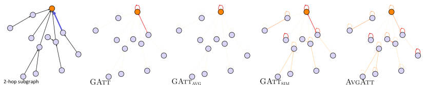
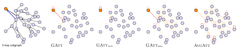
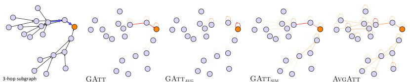
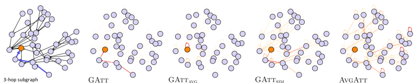
We conduct case studies on the BA-Shapes and Infection datasets for a 2-layer GAT, while visualizing how different methods behave. In Figure 3, each of two cases shows a randomly selected target node (marked as orange) and the edges in ground truth explanations (blue edges). We aim to observe how much the attribution scores from GAtt, GAtt ${}_{\textsc{avg}}$ and GAtt ${}_{\textsc{sim}}$ focus on the ground truth explanation edges. Indeed, for both datasets, GAtt focuses primarily on the edges in ground truth explanations, while the attribution scores from GAtt ${}_{\textsc{sim}}$ and AvgAtt tend to be more spread throughout the entire 2-hop local graph. This indicates that the attention weights in the GAT indeed recognize the ground truth explanations under GAtt calculations. In the case of GAtt ${}_{\textsc{avg}}$ , the attribution patterns are not much different from GAtt in BA-Shapes. However, GAtt ${}_{\textsc{avg}}$ in the Infection dataset attributes its attribution scores to a single self-loop edge that does not belong to the ground truth explanations, failing to provide adequate explanations. Interestingly, on BA-Shapes, GAtt tends to strongly emphasize edges that are closer in proximity even within the house-shaped motifs, which coincides with the pitfall addressed in (Faber, Moghaddam, and Wattenhofer 2021). Further extensive case studies including more target nodes and 3-layer models exhibit a similar tendency to Figure 3 (see Appendices E.1 and H for SuperGAT and GAT/GATv2, respectively).

4 Conclusion and Future work

In this study, we have investigated the largely underexplored problem of interpreting Att-GNNs. Although Att-GNNs were not considered as a candidate for inherently explainable models, our empirical evaluations have demonstrated affirmative results when our proposed method, GAtt, built upon the computation tree, can be used to effectively calculate edge attribution scores. Although GAtt is generally applicable, this work does not include a systematic analysis on how different designs of attention weights will interact with GAtt, which we leave for future work.

Acknowledgments

This work was supported by the National Research Foundation of Korea (NRF) grant funded by the Korea government (MSIT) (No. 2021R1A2C3004345, No. RS-2023-00220762).

References

Abnar and Zuidema (2020) Abnar, S.; and Zuidema, W. H. 2020. Quantifying Attention Flow in Transformers. In ACL, 4190–4197. Online.
Aflalo et al. (2022) Aflalo, E.; Du, M.; Tseng, S.; Liu, Y.; Wu, C.; Duan, N.; and Lal, V. 2022. VL-InterpreT: An Interactive Visualization Tool for Interpreting Vision-Language Transformers. In CVPR. New Orleans, LA.
Azzolin et al. (2023) Azzolin, S.; Longa, A.; Barbiero, P.; Liò, P.; and Passerini, A. 2023. Global Explainability of GNNs via Logic Combination of Learned Concepts. In ICLR. Kigali, Rwanda.
Bahdanau, Cho, and Bengio (2015) Bahdanau, D.; Cho, K.; and Bengio, Y. 2015. Neural Machine Translation by Jointly Learning to Align and Translate. In ICLR. San Diego, CA.
Baldassarre and Azizpour (2019.) Baldassarre, F.; and Azizpour, H. 2019. Explainability Techniques for Graph Convolutional Networks. In ICLR Workshop on Learning and Reasoning with Graph-Structured Data. Long Beach, CA.
Bibal et al. (2022) Bibal, A.; Cardon, R.; Alfter, D.; Wilkens, R.; Wang, X.; François, T.; and Watrin, P. 2022. Is Attention Explanation? An Introduction to the Debate. In ACL, 3889–3900. Dublin, Ireland.
Brocki and Chung (2023) Brocki, L.; and Chung, N. C. 2023. Class-Discriminative Attention Maps for Vision Transformers. CoRR, abs/2312.02364.
Brody, Alon, and Yahav (2022) Brody, S.; Alon, U.; and Yahav, E. 2022. How Attentive are Graph Attention Networks? In ICLR. Virtual Event.
Bronstein et al. (2021) Bronstein, M. M.; Bruna, J.; Cohen, T.; and Velickovic, P. 2021. Geometric Deep Learning: Grids, Groups, Graphs, Geodesics, and Gauges. arXiv:2104.13478.
Caron et al. (2021) Caron, M.; Touvron, H.; Misra, I.; Jégou, H.; Mairal, J.; Bojanowski, P.; and Joulin, A. 2021. Emerging Properties in Self-Supervised Vision Transformers. In ICCV, 9630–9640. Montreal, Canada.
Chefer, Gur, and Wolf (2021a) Chefer, H.; Gur, S.; and Wolf, L. 2021a. Generic Attention-model Explainability for Interpreting Bi-Modal and Encoder-Decoder Transformers. In ICCV, 387–396. Montreal, Canada.
Chefer, Gur, and Wolf (2021b) Chefer, H.; Gur, S.; and Wolf, L. 2021b. Transformer Interpretability Beyond Attention Visualization. In CVPR, 782–791. virtual.
Chen et al. (2023) Chen, J.; Gao, K.; Li, G.; and He, K. 2023. NAGphormer: A Tokenized Graph Transformer for Node Classification in Large Graphs. In ICLR.
Chrysostomou and Aletras (2021) Chrysostomou, G.; and Aletras, N. 2021. Improving the Faithfulness of Attention-based Explanations with Task-specific Information for Text Classification. In ACL/IJCNLP, 477–488. Virtual Event.
Debnath et al. (1991) Debnath, A. K.; Lopez de Compadre, R. L.; Debnath, G.; Shusterman, A. J.; and Hansch, C. 1991. Structure-activity relationship of mutagenic aromatic and heteroaromatic nitro compounds. Correlation with molecular orbital energies and hydrophobicity. J. Med. Chem., 34(2): 786–797.
Deiseroth et al. (2023) Deiseroth, B.; Deb, M.; Weinbach, S.; Brack, M.; Schramowski, P.; and Kersting, K. 2023. ATMAN: Understanding Transformer Predictions Through Memory Efficient Attention Manipulation. In NeurIPS. New Orleans, LA.
Dosovitskiy et al. (2021) Dosovitskiy, A.; Beyer, L.; Kolesnikov, A.; Weissenborn, D.; Zhai, X.; Unterthiner, T.; Dehghani, M.; Minderer, M.; Heigold, G.; Gelly, S.; Uszkoreit, J.; and Houlsby, N. 2021. An Image is Worth 16x16 Words: Transformers for Image Recognition at Scale. In ICLR. Virtual event.
Du, Liu, and Hu (2020) Du, M.; Liu, N.; and Hu, X. 2020. Techniques for interpretable machine learning. Commun. ACM, 63(1): 68–77.
Faber, Moghaddam, and Wattenhofer (2021) Faber, L.; Moghaddam, A. K.; and Wattenhofer, R. 2021. When Comparing to Ground Truth is Wrong: On Evaluating GNN Explanation Methods. In KDD, 332–341. Virtual Event.
Fang et al. (2020) Fang, X.; Huang, J.; Wang, F.; Zeng, L.; Liang, H.; and Wang, H. 2020. ConSTGAT: Contextual Spatial-Temporal Graph Attention Network for Travel Time Estimation at Baidu Maps. In KDD, 2697–2705. Virtual Event, CA.
Fountoulakis et al. (2023) Fountoulakis, K.; Levi, A.; Yang, S.; Baranwal, A.; and Jagannath, A. 2023. Graph Attention Retrospective. J. Mach. Learn. Res., 24: 246:1–246:52.
Ghaeini, Fern, and Tadepalli (2018) Ghaeini, R.; Fern, X. Z.; and Tadepalli, P. 2018. Interpreting Recurrent and Attention-Based Neural Models: a Case Study on Natural Language Inference. In EMNLP, 4952–4957. Brussels, Belgium.
Gilmer et al. (2017) Gilmer, J.; Schoenholz, S. S.; Riley, P. F.; Vinyals, O.; and Dahl, G. E. 2017. Neural Message Passing for Quantum Chemistry. In ICML, 1263–1272. Sydney, NSW.
Guo et al. (2017) Guo, C.; Pleiss, G.; Sun, Y.; and Weinberger, K. Q. 2017. On Calibration of Modern Neural Networks. In ICML, 1321–1330. Sydney, Australia.
Hao et al. (2021) Hao, Y.; Dong, L.; Wei, F.; and Xu, K. 2021. Self-Attention Attribution: Interpreting Information Interactions Inside Transformer. In AAAI, 12963–12971. Virtual event.
Hase, Xie, and Bansal (2021) Hase, P.; Xie, H.; and Bansal, M. 2021. The Out-of-Distribution Problem in Explainability and Search Methods for Feature Importance Explanations. In NeurIPS, 3650–3666. Virtual event.
Hooker et al. (2019) Hooker, S.; Erhan, D.; Kindermans, P.; and Kim, B. 2019. A Benchmark for Interpretability Methods in Deep Neural Networks. In NeurIPS, 9734–9745. Vancouver, Canada.
Hu et al. (2020) Hu, W.; Fey, M.; Zitnik, M.; Dong, Y.; Ren, H.; Liu, B.; Catasta, M.; and Leskovec, J. 2020. Open Graph Benchmark: Datasets for Machine Learning on Graphs. In NeurIPS. Virtual event.
Jacovi and Goldberg (2020) Jacovi, A.; and Goldberg, Y. 2020. Towards Faithfully Interpretable NLP Systems: How Should We Define and Evaluate Faithfulness? In ACL, 4198–4205. Online.
Jain and Wallace (2019) Jain, S.; and Wallace, B. C. 2019. Attention is not Explanation. In NAACL-HLT, 3543–3556. Minneapolis, MN.
Kim and Oh (2021) Kim, D.; and Oh, A. 2021. How to Find Your Friendly Neighborhood: Graph Attention Design with Self-Supervision. In ICLR. Virtual Event.
Knyazev, Taylor, and Amer (2019) Knyazev, B.; Taylor, G. W.; and Amer, M. R. 2019. Understanding Attention and Generalization in Graph Neural Networks. In NeruIPS. Vancouver, Canada.
Kreuzer et al. (2021) Kreuzer, D.; Beaini, D.; Hamilton, W. L.; Létourneau, V.; and Tossou, P. 2021. Rethinking Graph Transformers with Spectral Attention. In NeurIPS, 21618–21629. Virtual event.
Lee, Shin, and Kim (2017) Lee, J.; Shin, J.; and Kim, J. 2017. Interactive Visualization and Manipulation of Attention-based Neural Machine Translation. In EMNLP, 121–126. Copenhagen, Denmark.
Lee et al. (2019) Lee, J. B.; Rossi, R. A.; Kim, S.; Ahmed, N. K.; and Koh, E. 2019. Attention Models in Graphs: A Survey. ACM Trans. Knowl. Discov. Data, 13(6): 62:1–62:25.
Li et al. (2022) Li, P.; Yang, Y.; Pagnucco, M.; and Song, Y. 2022. Explainability in Graph Neural Networks: An Experimental Survey. arXiv:2203.09258.
Liu et al. (2022) Liu, Y.; Li, H.; Guo, Y.; Kong, C.; Li, J.; and Wang, S. 2022. Rethinking Attention-Model Explainability through Faithfulness Violation Test. In ICML, 13807–13824. Baltimore, MD.
Luo et al. (2020) Luo, D.; Cheng, W.; Xu, D.; Yu, W.; Zong, B.; Chen, H.; and Zhang, X. 2020. Parameterized Explainer for Graph Neural Network. In NeurIPS. Virtual event.
Miao, Liu, and Li (2022) Miao, S.; Liu, M.; and Li, P. 2022. Interpretable and Generalizable Graph Learning via Stochastic Attention Mechanism. In ICML. Baltimore, MD.
Michel, Levy, and Neubig (2019) Michel, P.; Levy, O.; and Neubig, G. 2019. Are Sixteen Heads Really Better than One? In NeurIPS, 14014–14024. Vancouver, Canada.
Moon et al. (2020) Moon, J.; Kim, J.; Shin, Y.; and Hwang, S. 2020. Confidence-Aware Learning for Deep Neural Networks. In ICML, 7034–7044. Vienna, Austria.
Morris et al. (2019) Morris, C.; Ritzert, M.; Fey, M.; Hamilton, W. L.; Lenssen, J. E.; Rattan, G.; and Grohe, M. 2019. Weisfeiler and Leman Go Neural: Higher-Order Graph Neural Networks. In AAAI, 4602–4609. Homolulu, HI.
Mouhah, Faiz, and Bourhnane (2023) Mouhah, K.; Faiz, H.; and Bourhnane, S. 2023. Large Matrix Multiplication Algorithms: Analysis and Comparison. In ICACS, 7–12. Larissa, Greece: ACM.
Mustafa, Bojchevski, and Burkholz (2023) Mustafa, N.; Bojchevski, A.; and Burkholz, R. 2023. Are GATs Out of Balance? In NeurIPS. New Orleans, LA.
Nguyen et al. (2021) Nguyen, T.; Le, H.; Quinn, T. P.; Nguyen, T.; Le, T. D.; and Venkatesh, S. 2021. GraphDTA: predicting drug-target binding affinity with graph neural networks. Bioinform., 37(8): 1140–1147.
Pei et al. (2020) Pei, H.; Wei, B.; Chang, K. C.; Lei, Y.; and Yang, B. 2020. Geom-GCN: Geometric Graph Convolutional Networks. In ICLR. Addis Ababa, Ethiopia.
Pereira et al. (2023) Pereira, T. A.; Nascimento, E.; Resck, L. E.; Mesquita, D.; and Souza, A. H. 2023. Distill n’ Explain: explaining graph neural networks using simple surrogates. In AISTATS. Palau de Congressos, Spain.
Pope et al. (2019) Pope, P. E.; Kolouri, S.; Rostami, M.; Martin, C. E.; and Hoffmann, H. 2019. Explainability Methods for Graph Convolutional Neural Networks. In CVPR, 10772–10781. Long Beach, CA.
Rensink (2000) Rensink, R. 2000. The Dynamic Representation of Scenes. Visual Cognition, 7: 17–42.
Sánchez-Lengeling et al. (2020) Sánchez-Lengeling, B.; Wei, J. N.; Lee, B. K.; Reif, E.; Wang, P.; Qian, W. W.; McCloskey, K.; Colwell, L. J.; and Wiltschko, A. B. 2020. Evaluating Attribution for Graph Neural Networks. In NeurIPS. virtual.
Sato, Yamada, and Kashima (2021) Sato, R.; Yamada, M.; and Kashima, H. 2021. Random Features Strengthen Graph Neural Networks. In SDM, 333–341. Virtual event.
Schlichtkrull, Cao, and Titov (2021) Schlichtkrull, M. S.; Cao, N. D.; and Titov, I. 2021. Interpreting Graph Neural Networks for NLP With Differentiable Edge Masking. In ICLR. Virtual Event.
Simonyan, Vedaldi, and Zisserman (2014) Simonyan, K.; Vedaldi, A.; and Zisserman, A. 2014. Deep Inside Convolutional Networks: Visualising Image Classification Models and Saliency Maps. In ICLR. Banff, Canada.
Springenberg et al. (2015) Springenberg, J. T.; Dosovitskiy, A.; Brox, T.; and Riedmiller, M. A. 2015. Striving for Simplicity: The All Convolutional Net. In ICLR. San Diego, CA.
Sun et al. (2023) Sun, C.; Li, C.; Lin, X.; Zheng, T.; Meng, F.; Rui, X.; and Wang, Z. 2023. Attention-based graph neural networks: a survey. Artif. Intell. Rev., 56(S2): 2263–2310.
Sundararajan, Taly, and Yan (2017) Sundararajan, M.; Taly, A.; and Yan, Q. 2017. Axiomatic Attribution for Deep Networks. In ICML. Sydney, Australia.
Tomsett et al. (2020) Tomsett, R.; Harborne, D.; Chakraborty, S.; Gurram, P.; and Preece2, A. 2020. Sanity Checks for Saliency Metrics. In AAAI. New York, NY.
Vaswani et al. (2017) Vaswani, A.; Shazeer, N.; Parmar, N.; Uszkoreit, J.; Jones, L.; Gomez, A. N.; Kaiser, L.; and Polosukhin, I. 2017. Attention is All you Need. In NIPS, 5998–6008. Long Beach, CA.
Velickovic et al. (2018) Velickovic, P.; Cucurull, G.; Casanova, A.; Romero, A.; Liò, P.; and Bengio, Y. 2018. Graph Attention Networks. In ICLR. Vancouver, Canada.
Vig (2019) Vig, J. 2019. A Multiscale Visualization of Attention in the Transformer Model. In ACL, 37–42. Florence, Italy.
Wiegreffe and Pinter (2019) Wiegreffe, S.; and Pinter, Y. 2019. Attention is not not Explanation. In EMNLP-IJCNLP, 11–20. Hong Kong, China.
Wu et al. (2019) Wu, F.; Jr., A. H. S.; Zhang, T.; Fifty, C.; Yu, T.; and Weinberger, K. Q. 2019. Simplifying Graph Convolutional Networks. In ICML. Long Beach, CA.
Wu et al. (2021) Wu, Z.; Pan, S.; Chen, F.; Long, G.; Zhang, C.; and Yu, P. S. 2021. A Comprehensive Survey on Graph Neural Networks. IEEE Trans. Neural Networks Learn. Syst., 32(1): 4–24.
Xu et al. (2015) Xu, K.; Ba, J.; Kiros, R.; Cho, K.; Courville, A. C.; Salakhutdinov, R.; Zemel, R. S.; and Bengio, Y. 2015. Show, Attend and Tell: Neural Image Caption Generation with Visual Attention. In ICML, 2048–2057. Lille, France.
Yang, Cohen, and Salakhutdinov (2016) Yang, Z.; Cohen, W. W.; and Salakhutdinov, R. 2016. Revisiting Semi-Supervised Learning with Graph Embeddings. In ICML. New York City, NY.
Ying et al. (2021) Ying, C.; Cai, T.; Luo, S.; Zheng, S.; Ke, G.; He, D.; Shen, Y.; and Liu, T. 2021. Do Transformers Really Perform Badly for Graph Representation? In NeurIPS, 28877–28888. virtual.
Ying et al. (2019) Ying, Z.; Bourgeois, D.; You, J.; Zitnik, M.; and Leskovec, J. 2019. GNNExplainer: Generating Explanations for Graph Neural Networks. In NeurIPS, 9240–9251. Vancouver, Canada.
Yuan et al. (2023) Yuan, H.; Yu, H.; Gui, S.; and Ji, S. 2023. Explainability in Graph Neural Networks: A Taxonomic Survey. IEEE Trans. Pattern Anal. Mach. Intell., 45(5): 5782–5799.

Appendix for ‘Faithful and Accurate Self-Attention Attribution for Message Passing Neural Networks via the Computation Tree Viewpoint’

List of Additional Experiments

◼

Runtime comparison among different calculations of GAtt: Appendix C
◼

Further applications of GAtt to other Att-GNN models (using SuperGAT): Appendix E.1
◼

Comprehensive expansion results of results from the main manuscript (GAT, GATv2, and ablation study): Appendix E.2
◼

Further experiments for multi-head attention: Appendix E.3
◼

Effect of regularization during training: Appendix E.4
◼

Experiments on graph-level tasks: Appendix E.5
◼

Empirical observations on the proximity effect: Appendix E.6
◼

Runtime comparison among different explanation methods: Appendix E.7
◼

Further visualizations of faithfulness for GAtt, $\textsc{GAtt}_{\textsc{sim}}$ , and AvgAtt: Appendix E.8
◼

Further case studies via visualizations: Appendices H (for GAT and GATv2) and E.1 (for SuperGAT)

Table of Notations

Notation	Description
$G$	A given graph
$\mathcal{V}$	The set of nodes
$\mathcal{E}$	The set of edges
$\mathcal{N}_{i}$	The set of neighbors of node $v_{i}$
$L$	The number of layers in the Att-GNN
$\mathcal{A}=\{{\bf A}(l)\}_{l=1}^{L}$	The set of attention weights in a $L$ -layer Att-GNN
${\bf A}(l)$	The attention weight matrix for the $l$ -th layer in Att-GNN
$\alpha_{i,j}=[{\bf A}(l)]_{j,i}$	The attention weight of $e_{i,j}$ in the $l$ -th layer in the Att-GNN
$\Phi$	The edge attribution function
$\phi_{i,j}^{v}$	The edge attribution score of $e_{i,j}$ for a target node $v$
$\lambda_{i,j,v}^{l}$	The list of edges of length $l$ starting from $e_{i,j}$ and ending with the root node $v$ within the computation tree
$\Lambda_{v}^{m}(e_{i,j})$	The set of all flows that starts from $e_{i,j}$ with length $m\in[1,L]$ for node $v$
$\alpha[\lambda_{v_{0},v_{1},w}^{m}]$	The list of attention weights corresponding to $\lambda_{v_{0},v_{1},w}^{m}$ in the Att-GNN
${\bf p}_{v}$	The output probability vector of Att-GNN for node $v$

Appendix A Related Work

In this section, we discuss previous relevant studies on two major themes. Specifically, we first address previous attempts to use attention weights as interpretations in domains other than graphs, and then we provide an overview of explainable AI (XAI) for GNNs.

Interpreting models with attention.

There have been a handful of studies that utilize attention as a tool for model interpretations. The term ‘attention’ itself refers to the biological inspiration of the design where human vision also relies on a dynamic focusing on relevant parts of real-world scenery (Rensink 2000; Bibal et al. 2022). This intuition is directly reflected in how the attention mechanism plays a role in machine learning models in general, namely to adjust the flow of information and to allow some parts of the input / latent representations, while the adjustment itself is a learned function of the input/latent representations (Bahdanau, Cho, and Bengio 2015; Vaswani et al. 2017). Aside from the performance benefits of attention, this role of attention within the model of interest makes attention a good conceptual fit to explain decisions. After all, it is much more natural for a sufficiently trained model to transfer the critical parts of the input (to the next layer) by assigning higher attention scores rather than vice versa (which can also be applied analogously to the human case). This in turn suggests that attention can be used to discover critical parts of the input that affected the model’s decisions, and therefore being an effective proxy of the model’s inner mechanism.

In machine learning, the attention mechanism has been used as model interpretations since its early development, typically as an intuitive visualization tool that highlights the inner workings of the underlying model (Bahdanau, Cho, and Bengio 2015; Xu et al. 2015; Vig 2019; Dosovitskiy et al. 2021; Caron et al. 2021). As attention usage as interpretations become more widespread, there have been multiple studies that extensively scrutinize attention explainability in the domain of natural language processing (NLP) (Bibal et al. 2022). In (Jain and Wallace 2019), attention was found to have low correlations with other attribution methods. However, (Wiegreffe and Pinter 2019) pointed out an unfair setting in the previous work and argued that attention can still be an effective explanation. Furthermore, there have been studies that focused on post-processing attention in transformers for token attributions. (Abnar and Zuidema 2020) proposed attention rollout and attention flow, and follow-up studies (Chefer, Gur, and Wolf 2021b, a; Hao et al. 2021) incorporate other attribution calculation methods or gradients with attention weights. Although our study lies in a similar objective, our focus is on graph data with the Att-GNN architecture, where attention has been mostly used as a naïve baseline and has been largely under-explored in the literature (Ying et al. 2019; Luo et al. 2020; Sánchez-Lengeling et al. 2020).

Explainability in GNNs.

The primary goal of XAI is to provide a comprehensive understanding of the decision of neural networks. Early works of explaining GNNs involved applying previously developed XAI methods (e.g., Saliency (Simonyan, Vedaldi, and Zisserman 2014), Integrated gradients (Sundararajan, Taly, and Yan 2017), Guided backpropagation (Springenberg et al. 2015)) directly to the underlying GNN model (Pope et al. 2019; Baldassarre and Azizpour 2019.) In recent years, various studies have developed explanation methods tailored to GNN models. As one of the pioneering work, GNNExplainer (Ying et al. 2019) identified a subset of edges and node features around the target node that affect the underlying model’s decision. PGExplainer (Luo et al. 2020) trained a separate parameterized mask predictor to generate edge masks that identify important edges. However, many approaches typically necessitate an optimization/learning framework, making the explanation performance dependent on various hyperparameters (e.g., the number of iterations and random seeds). GraphMask (Schlichtkrull, Cao, and Titov 2021) learns a single-layer MLP classifier to predict whether an edge in each layer can be replaced by a learned baseline vector. Finally, FastDnx (Pereira et al. 2023) first performs knowledge distillation in a surrogate SGC model, where the explanation is eventually retrieved by solving a simple convex program. However, recent analysis demonstrated that such explanations are also known to be suboptimal, as they essentially perform a single step projection to an information-controlled space, and their high dependency on optimization and learning makes them prone to being sensitive to random seeds (Miao, Liu, and Li 2022). Although explanations of GNN models are still an active research area (Li et al. 2022; Yuan et al. 2023), most studies overlooked attention as a powerful method for explanations. Several studies (Ying et al. 2019; Luo et al. 2020; Sánchez-Lengeling et al. 2020) have introduced GATs, a representative model in Att-GNNs, as a baseline by averaging attention over layers. In light of this, our study aims to scrutinize attention as a paramount candidate to explain Att-GNNs, and develop a simple attribution method based on attention that avoids the pitfalls of previous GNN explainability methods by being deterministic (do not require random seeds) and avoiding the usage of hyperparameters.

Appendix B Experimental Settings

B.1 Dataset Description and Statistics

We provide a more detailed description of the synthetic datasets used in Section 3.2.

Table 6: Statstics for the synthetic datasets used in the experiments.

Dataset	Num. nodes	Num. edges	Num. features	Num. classes	Num. motifs	Num. unique explanations
BA-Shapes	700	1,426	50	4	80	-
Infection (2-layer GAT)	5,000	10,086	2	4	-	1,057
Infection (3-layer GAT)	5,000	10,086	2	5	-	974

Table 7: Statstics for the real-world datasets used in the experiments.

Dataset	Num. nodes	Num. edges	Num. features	Num. classes
Cora	2,708	10,556	1,433	7
Citeseer	3,327	9,104	3.703	6
Pubmed	19,717	88,648	500	3
Arxiv	169,343	1,166,243	128	40
Cornell	183	295	1703	5
Texas	183	309	1703	5
Wisconsin	251	499	1703	5

◼

BA-shapes (Ying et al. 2019) is a synthetic graph that attaches 80 house-shaped motifs to a base graph made from the Barabási-Albert model with 300 nodes. The task is to classify whether a node belongs to one of four cases, including the top, middle, and bottom of a house, or the base graph. The edges belonging to the house-shaped motifs is regarded as the ground truth explanation. We use the one-hot encodings of each node’s degree as the node features to ease the training.
◼

Infection benchmark (Faber, Moghaddam, and Wattenhofer 2021) is also a synthetic dataset where the backbone graph is generated from the Erdös-Rényi model. Then, a small portion of the nodes are assigned to ‘infected’, where the information is encoded as a one-hot vector as a node feature (indicating ‘infected’ versus ‘normal’). The node label is set as either 1) ‘infected’ or 2) the length of the shortest path to the nearest infected node, if not infected. For an $L$ -layer Att-GNN, all nodes that are more than $L$ -hops away from the nearest infected node are considered as the same class. The ground truth explanation for the infection benchmark graph is the edges along the path from the nearest infected node to the target node. During evaluations, we only observe the performance of edge attribution calculation methods on nodes with a unique ground truth path (as suggested by the original authors). The number of unique explanations indicates the number of nodes having the unique shortest path to the nearest infected node.

In addition, we summarize the statistics of the synthetic and real-world datasets used in our experiments in Tables 6 and 7, respectively. Cora, Citeseer, Pubmed (Yang, Cohen, and Salakhutdinov 2016) and Arxiv (Hu et al. 2020) are citation network where each node represents a paper, and an edge represents a citation between two papers. These four datasets are homophilic, i.e., nodes that belong to the same class have a higher probability to be connected. On the other hand, Cornell, Texas, and Wisconsin (Pei et al. 2020) is part of the WebKD dataset, which is a web page network collected from computer science departments of various universities. For these datasets, nodes represent web pages and edges represent hyperlinks between the web pages. Also, these three datasets are heterophilic, i.e., nodes that belong to different classes are likely to be connected.

B.2 Training Details of GAT/GATv2s in Experiments

Table 8: Training details for different datasets used in the experiment.

		BA-Shapes	Infection	Cora	Citeseer	Pubmed	Arxiv	Cornell	Texas	Wisconsin
	Num. epochs	1000	500	60	100	100	3000	65	32	50
GAT	Hidden dim.	16	8	64	64	64	64	64	64	64
(2 layer)	Learning rate	0.01	0.005	0.001	0.001	0.001	0.005	0.005	0.001	0.0001
	Test acc.	0.9500	0.8680	0.8202	0.7312	0.7294	0.5375	0.5135	0.5676	0.5098
	Num. epochs	1000	500	60	100	100	3000	65	32	50
GAT	Hidden dim.	16	8	64	64	64	64	64	64	64
(3 layer)	Learning rate	0.01	0.005	0.001	0.001	0.001	0.005	0.005	0.001	0.0001
	Test acc.	0.9571	0.9272	0.8362	0.7272	0.7885	0.5188	0.5135	0.6216	0.5098
	Num. epochs	1000	1000	60	60	60	3000	100	32	50
GATv2	Hidden dim.	16	16	64	64	64	64	64	64	64
(2 layer)	Learning rate	0.01	0.01	0.001	0.001	0.001	0.005	0.001	0.001	0.0001
	Test acc.	0.9357	0.9476	0.8292	0.7275	0.7157	0.5290	0.4865	0.4054	0.4314
	Num. epochs	1000	1000	60	60	60	3000	100	32	50
GATv2	Hidden dim.	16	16	64	64	64	64	64	64	64
(3 layer)	Learning rate	0.01	0.01	0.001	0.001	0.001	0.005	0.001	0.001	0.0001
	Test acc.	0.9714	0.9992	0.7644	0.7286	0.7197	0.5243	0.4054	0.4865	0.4902

Table 8 summarizes the number of epochs, hidden dimension, learning rate, and the test accuracy for each model (i.e., GAT/GATv2) and dataset used in the experiments. Furthermore, we describe the detailed settings regarding data splits. For the synthetic datasets, we split the nodes into training and test sets with the ratio of 50:50. For the real-world citation datasets, we randomly select 100 nodes per class to form a training set, and consider the rest of the nodes as test sets. Finally, we use the Adam optimizer for all cases.

B.3 Implementation Specifications

We use Python 3.10.12, with Pytorch 2.0.1, and Pytorch Geometric 2.3.1 (We use Pytorch Geometric 2.5.2 only when GraphMask (Schlichtkrull, Cao, and Titov 2021) is required). The experiments were run on a machine with an Intel(R) Core(TM) i7-10700K CPU @ 3.80GHz, 64GB of RAM, and a single Nvidia GeForce RTX 3080 graphics card.

Appendix C Batch Calculation of GAtt

# A(i): Attention weight matrix for the i-th layer, i = 1, ..., L

# v: target node

select_matrix = torch.zeros_like(A(1))

select_matrix[v, :] = 1

GAtt = select_matrix * A(L)

for i in range(1, L):

GAtt += C(L-i)[v, :].expand_as(A(1)).t() * A(i)

Algorithm 1 PyTorch-style pseudocode for batch calculation of GAtt

Recall that Proposition 2.5 basically represents a matrix-based computation of GATT for an $L$ -layer GAT. As mentioned in Section 2.3, we can pre-compute ${\bf C}(1),\cdots,{\bf C}(L-1)$ , which can be reused when GAtt is calculated for any edge $e_{i,j}$ . This approach is efficient for calculating GAtt for a single edge, but is still inefficient in computing GAtt for a batch of edges. Here, we provide a PyTorch-style pseudocode for GAtt in Algorithm 1 that is more suited for batch computations.

Since GAtt in Algorithm 1 is a torch.Tensor object, we can acquire the attribution values according to GAtt simply by retrieving the values of the proper index (i.e., $\phi^{v}_{i,j}=$ GAtt[j,i]).

To empirically show the effectiveness of Algorithm 1 (i.e., batch-based GAtt calculation), we carry out an experiment in which the runtime of calculating GAtt is measured for the target nodes in the Infection dataset (974 nodes in total). As shown in Figure 4, the results clearly reveal that, in the batch computation strategy, using Algorithm 1 is much preferred compared to the other two calculation strategies, including calculations based on a rooted subtree and a matrix-based calculation using Eq. (3). For a runtime comparison of the batch computation against other edge attribution methods, we refer to Appendix E.7.

Appendix D Overview of Attention

D.1 Self-Attention

In the transformer model, self-attention (Vaswani et al. 2017) has been regarded as the key module that not only brings performance benefits but also provides interpretations of the model. In this subsection, we describe the core component of the self-attention module.

We assume that we are given $n$ input tokens with $d^{\prime}$ -dimensions ${\bf T}\in\mathbb{R}^{n\times d^{\prime}}$ . In self-attention, we calculate the attention weights by first linearly transforming ${\bf T}$ into three different representations (of the same resulting dimensions), including the matrices of query ${\bf Q}$ , key ${\bf K}$ , and the value ${\bf V}$ , which are defined as ${\bf Q}={\bf TW}_{Q}$ , ${\bf K}={\bf TW}_{K}$ , and ${\bf V}={\bf TW}_{V}$ , where ${\bf W}_{Q}$ , ${\bf W}_{K}$ , and ${\bf W}_{V}$ are learnable parameters. Then, each query representation is compared to the key representation of all other input tokens in the same set (hence ‘self’) to calculate how much it should attend to other parts of the input during computation. In other words, we generate a query-dependent distribution of attention scores. This process can be neatly expressed as follows:

\text{SelfAttention}({\bf Q,K,V})=\text{softmax}\left(\dfrac{{\bf QK}^{\top}}{\sqrt{d_{a}}}\right){\bf V},

(6)

where $d_{a}$ is the dimension of the tokens after initial linear transformation, and the softmax function is applied row-wise.

D.2 Attention-based GNNs

Message passing neural networks (MPNN).

GNNs adopt the message passing mechanism as the building block of each layer, which enables GNNs to naturally encode the graph structure to the node representations. The representation ${\bf h}_{v}^{(l)}$ of node $v$ in the $l$ -th layer of GNNs is calculated as

{\bf h}_{v}^{(l+1)}=\textsc{Readout}\left({\bf h}_{v}^{(l)},\bigoplus_{u\in\mathcal{N}_{v}}\textsc{Message}({\bf h}_{v}^{(l)},{\bf h}_{u}^{(l)})\right),

(7)

where Message is the message function computed for each edge $e_{v,u}$ , $\bigoplus$ is the permutation invariant aggregation function (e.g., summation), and Readout is the readout function that takes the representation of node $v$ and the aggregated message to return a new representation. Note that the recursive design of Eq. (7) has a unique consequence on the actual computation in GNNs; for an $L$ -layer GNN, the calculation for node $v$ is essentially encoding a rooted subtree of height $L$ , with $v$ at its root (Morris et al. 2019). A popular variant of MPNN incorporates the self-attention mechanism into the message passing mechanism. Due to the effectiveness and unique interpretation potential of attention, such attention-based MPNNs (Att-GNNs) have been separately investigated by the literature (refer to the introduction for detailed discussion). Among those models, we focus on the following three Att-GNNs as the representative architecture.

GAT.

GATs incorporate the concept of self-attention in message passing. The key idea is to treat the set of input tokens in the original self-attention as the hidden representations of nodes in $\mathcal{N}_{i}\cup\{i\}$ , where $\mathcal{N}_{i}$ is the set of neighbors of node $i$ . Specifically, the $l$ -th graph attention layer of GATs is given by (Velickovic et al. 2018):

{\bf h}_{i}^{(l+1)}=\sum_{j\in\mathcal{N}_{i}\cup\{i\}}\alpha_{j,i}{\bf h}_{j}^{(l)},

(8)

where the attention weight $\alpha_{j,i}$ is defined as $\text{softmax}(\text{LeakyReLU}({\bf a}^{\top}[{\bf W}{\bf h}_{j}||{\bf W}{\bf h}_{i}]))$ for learnable parameters ${\bf a}$ and ${\bf W}$ . Conceptually, nodes $i$ and $j$ are considered as queries and keys, respectively, which determine the attention weights $\alpha_{j,i}$ in Eq. (8), and ${\bf h}_{j}^{(l)}$ is considered as values.

GATv2.

We also describe the attention layer in GATv2 (Brody, Alon, and Yahav 2022). GATv2 is a modified architecture of GAT by improving upon the self-attention module to increase the model expressiveness. The difference between the two models can be summarized by the following two equations expressing the attention coefficient $e({\bf h}_{i},{\bf h}_{j})$ :

	$\displaystyle\text{GAT: }e({\bf h}_{i},{\bf h}_{j})$	$\displaystyle=\text{LeakyReLU}({\bf a}^{\top}[{\bf W}{\bf h}_{i}\|\|{\bf W}{\bf h}_{j}]),$		(9)
	$\displaystyle\text{GATv2: }e({\bf h}_{i},{\bf h}_{j})$	$\displaystyle={\bf a}^{\top}\text{LeakyReLU}({\bf W}[{\bf h}_{i}\|\|{\bf h}_{j}]),$		(10)

where ${\bf a}$ and ${\bf W}$ are learnable parameters and ${\bf h}_{i}$ is the intermediate representation of node $i$ . Despite the different self-attention mechanisms, the structure of the computation tree is essentially identical to that of GAT. Therefore, the application of GAtt to GATv2 is fairly straightforward.

SuperGAT.

There exists two advanced variants of SuperGAT (Kim and Oh 2021), namely $\text{SuperGAT}_{\text{SD}}$ and $\text{SuperGAT}_{\text{MX}}$ . For $\text{SuperGAT}_{\text{SD}}$ , the unnormalized attention coefficient is calculated by scaling down the dot-product version of attention:

\text{SuperGAT}_{\text{SD}}:e({\bf h}_{i},{\bf h}_{j})=\dfrac{1}{\sqrt{F}}({\bf W}{\bf h}_{i})^{\top}\cdot({\bf W}{\bf h}_{j}),

(11)

where $F$ denotes the dimension of ${\bf h}_{i}$ and ${\bf h}_{j}$ , ${\bf a}$ and ${\bf W}$ are learnable parameters, and ${\bf h}_{i}$ is the intermediate representation of node $i$ . On the other hand, the unnormalized attention for $\text{SuperGAT}_{\text{MX}}$ is the product between the original GAT attention coefficient and the dot-product version:

\text{SuperGAT}_{\text{MX}}:e({\bf h}_{i},{\bf h}_{j})=\text{LeakyReLU}({\bf a}^{\top}[{\bf W}{\bf h}_{j}||{\bf W}{\bf h}_{i}]))\cdot\sigma(({\bf W}{\bf h}_{i})^{\top}\cdot({\bf W}{\bf h}_{j})),

(12)

where $\sigma$ denotes the sigmoid function. Similar as to the case with GATv2, the application of GAtt to SuperGAT is straightforward since the structure of the computation tree is identical.

D.3 Comparison of Computation Trees Between Att-GNNs and Transformers

Although both Att-GNNs and transformers employ self-attention as the core module of their architectures, the way we consider how the computation trees of Att-GNNs are taken into consideration is different from the case of how transformers are analyzed (Abnar and Zuidema 2020; Chefer, Gur, and Wolf 2021b, a). Despite the existence of multiple transformer architectures that have been proposed for graph learning (which are also known as graph transformers) (Ying et al. 2021; Kreuzer et al. 2021; Chen et al. 2023), the self-attention module still generally follows the original one in (Vaswani et al. 2017). In this subsection, we discuss the differences between how the computation tree is described for Att-GNNs and how the computation process of graph transformers is discussed during model analysis. To this end, we use a vanilla version of graph transformers where each input token represents a node in the underlying graph.

Figure 5 illustrates the typical computation trees for a 3-layer GAT and the first 2 layers of a graph transformer given an example graph when the target node 0 is given. Before the analysis, we observe the following critical difference between Att-GNNs and graph transformers:

◼

Att-GNNs handle the edges existing only in the underlying graph, while graph transformers use a fully-connected graph for the self-attention in general.

Often, due to this characteristic, a typical challenge for graph transformers is developing an effective way to inject structural information into the self-attention module as additional features (Chen et al. 2023). Additionally, this is the root cause for most of the points that arise regarding the comparison between Att-GNNs and graph transformers. Specifically, we will analyze the computation tree of the (vanilla) graph transformer in Figure 5(c) by reflecting on our own observations in Section 2.3, which we make as follows:

(O1)

“(For Att-GNNs) Identical edges can appear multiple times in the computation tree”: This is not the case when we look at each layer of the computation tree of the graph transformer, since each edge is represented once per layer. For example, the self-loop of node 0 appears once per layer in Figure 5(c), while it appears twice in Figure 5(b) at the bottom level.
(O2)

“(For Att-GNNs) Nodes do not appear uniformly in the computation tree. Specifically, nodes that are $k$ -hops away from the target node do not exist in depth $k^{\prime}$ for $0<k^{\prime}<k$ ”: This is also not the case for graph transformers, since all edges are represented over all layers in the computation tree. For example, edge $e_{2,3}$ appears for all layers in Figure 5(c), while it appears in Figure 5(b) only at the bottom level for the case of GAT.
(O3)

“(For Att-GNNs) The graph attention layer always includes self-loops during its feed-forward process”: This is the only point that holds for both Att-GNNs and graph transformers.

From the analysis above, we require a different approach for the computation tree viewpoint, apart from previous studies that attempted to interpret transformer models using attention weights (Jain and Wallace 2019; Wiegreffe and Pinter 2019; Bibal et al. 2022; Abnar and Zuidema 2020; Chefer, Gur, and Wolf 2021b, a).

Appendix E Further Experimental Results

We include the experimental results that were not shown in the main manuscript.

E.1 Further Experiments Using SuperGAT (Table 9, Figure 6)

Table 9: Experimental results on both variants of SuperGAT with respect to the faithfulness for GAtt, AvgAtt, and random attribution on the Cora dataset. Results for 2-layer and 3-layer SuperGATs are shown for each case. The best performer is highlighted as bold.

Model	Measure	Metric		2-layer			3-layer
Model	Measure	Metric	GAtt	AvgAtt	Random	GAtt	AvgAtt	Random
$\text{SuperGAT}_{\text{MX}}$	$\Delta_{\text{PC}}$	$\rho_{\text{Pearson}}$ ( $\uparrow$ )	0.1345	0.0207	-0.0030	0.1209	0.0070	-0.0003
		$\tau_{\text{Kendall}}$ ( $\uparrow$ )	-0.0783	0.0413	-0.0095	-0.0330	-0.0006	-0.0004
		$\rho_{\text{Spearman}}$ ( $\uparrow$ )	-0.0790	0.0606	-0.0131	-0.0273	-0.0008	-0.0006
	$\Delta_{\text{NE}}$	$\rho_{\text{Pearson}}$ ( $\uparrow$ )	0.1124	0.0173	-0.0009	0.1101	0.0062	0.0022
		$\tau_{\text{Kendall}}$ ( $\uparrow$ )	-0.0823	0.0510	0.0011	-0.0153	-0.0004	-0.0001
		$\rho_{\text{Spearman}}$ ( $\uparrow$ )	-0.0831	0.0713	0.0015	-0.0108	0.0000	-0.0001
	$\Delta_{\text{P}}$	AUROC ( $\uparrow$ )	0.9808	0.5794	0.5131	0.9893	0.6269	0.5299
$\text{SuperGAT}_{\text{SD}}$	$\Delta_{\text{PC}}$	$\rho_{\text{Pearson}}$ ( $\uparrow$ )	0.1659	0.0329	0.0017	0.1199	0.0117	-0.0008
		$\tau_{\text{Kendall}}$ ( $\uparrow$ )	-0.0294	0.0404	0.0078	0.0012	-0.0013	-0.0013
		$\rho_{\text{Spearman}}$ ( $\uparrow$ )	-0.0275	0.0562	0.0110	0.0085	-0.0017	-0.0019
	$\Delta_{\text{NE}}$	$\rho_{\text{Pearson}}$ ( $\uparrow$ )	0.1478	0.0305	0.0050	0.1094	0.0114	0.0003
		$\tau_{\text{Kendall}}$ ( $\uparrow$ )	-0.0250	0.0322	0.0043	0.0018	-0.0077	0.0004
		$\rho_{\text{Spearman}}$ ( $\uparrow$ )	-0.0226	0.0458	0.0060	0.0118	-0.0102	0.0006
	$\Delta_{\text{P}}$	AUROC ( $\uparrow$ )	0.9820	0.5692	0.3942	0.9886	0.6877	0.2744

We perform an additional experiment by applying GAtt to SuperGAT (Kim and Oh 2021), another widely used Att-GNN model to demonstrate the general applicability. SuperGAT offers two types of attention variants, namely $\text{SuperGAT}_{\text{SD}}$ and $\text{SuperGAT}_{\text{MX}}$ , according to the ways of calculating the attention weights. Specifically, $\text{SuperGAT}_{\text{SD}}$ employs a scaled dot-product attention design, while $\text{SuperGAT}_{\text{MX}}$ utilizes both the original attention from GAT and dot-product attention (We refer to Appendix D.2 for a more formal description). To empirically observe the performance of GAtt, we train 2-layer and 3-layer SuperGATs with a single attention head for both attention variants on the Cora dataset, each of which achieves the test accuracy of $>0.76$ .

Table 9 summarizes the results of comparing GAtt with AvgAtt and random attribution with respect to the faithfulness on the Cora dataset. Although the correlation measures (i.e., $\Delta_{\text{PC}}$ and $\Delta_{\text{NE}}$ ) are generally weaker compared to the case of GATs, GAtt shows better faithfulness in terms of $\rho_{\text{Pearson}}$ and AUROC.

Furthermore, we performed additional case studies on the BA-Shapes and Infection datasets to visualize the effect of edge attribution methods on SuperGATs. Figure 6 shows visualizations of the edge attribution calculation scores using GAtt, GAtt ${}_{\textsc{avg}}$ , GAtt ${}_{\textsc{sim}}$ , and AvgAtt on node 600 in BA-Shapes and on node 2 in Infection. We observe similar tendencies to those of GAT and GATv2 on BA-Shapes (see Figures 11 and 13). However, we observe that the edge attributions for both variants of SuperGAT do not reveal the ground truth explanations as stongly as GAT or GATv2, especially on the Infection dataset. This implies that the behavior of GAtt is likely to be affected by the underlying model architecture itself. As mentioned in Section 4, we leave the analysis of the interactions between GAtt and the design of different types of attention for future work.

E.2 Expanded Results from the Main Manuscript (Tables 10–12)

We comprehensively show the experimental results of the faithfulness for GAT and GATv2 in the main manuscript by expanding Table 2 by including Kendall’s tau ( $\tau_{\text{Kendall}}$ ) and Spearman’s rho ( $\rho_{\text{Spearman}}$ ) alongside Pearson’s rho ( $\rho_{\text{Pearson}}$ to measure $\Delta_{\text{PC}}$ and $\Delta_{\text{NE}}$ . Tables 11 and 12 summarize the entire set of experimental results for GAT and GATv2, respectively. From Table 11, it is shown that, when GAT is used, GAtt achieves superior performance compared to AvgAtt and random attribution in most cases. However, in Table 12, we observe that the results for GATv2 are weaker for $\Delta_{\text{PC}}$ and $\Delta_{\text{NE}}$ compared to the case of GAT and are less consistent in terms of $\tau_{\text{Kendall}}$ and $\rho_{\text{Spearman}}$ for Pubmed and Arxiv datasets. This is due to the difference in the model architecture, as the attention weights in GAT are static in the sense that the ranking of the attention weights is independent of the query node. This characteristic of GAT serves as an advantage in terms of the correlation between the edge attributions and the model output, as the attention weights behave more predictively compared to GATv2. Finally, we would like to emphasize that the performance of GAtt is still vastly superior in terms of $\Delta_{\text{P}}$ , since this is the most important measurement in practice as it predicts whether the model will actually change its prediction after attention reduction.

Table 10: Performance comparison among different edge attribution calculation methods for GATs.

Dataset	Model	GAtt	GAtt ${}_{\textsc{sim}}$	GAtt ${}_{\textsc{avg}}$	AvgAtt
Cora	2-layer	0.7793	0.7565	0.7650	0.0461
Cora	3-layer	0.7598	0.6603	0.6940	0.0954
Citeseer	2-layer	0.8514	0.8295	0.7317	0.1995
Citeseer	3-layer	0.8019	0.7210	0.7890	0.1734
Pubmed	2-layer	0.7792	0.7413	0.6796	0.1158
Pubmed	3-layer	0.7136	0.5727	0.7051	0.0721

Furthermore, we also provide a more comprehensive result from the ablation study in Table 5. Table 10 summarizes the results by averaging over all 7 measures and metrics (i.e., Kendall’s tau ( $\tau_{\text{Kendall}}$ ) and Spearman’s rho ( $\rho_{\text{Spearman}}$ ) for $\Delta_{\text{PC}}$ and $\Delta_{\text{NE}}$ , and AUROC for $\Delta_{\text{P}}$ ). The results show the same performance trend, where the variants of GAtt and AvgAtt performs worse for all 2 and 3-layer cases.

Table 11: Experimental results with respect to the faithfulness for GAtt, AvgAtt, and random attribution on four real-world datasets. Results for 2-layer and 3-layer GATs are shown for each case. The best performer is highlighted as bold.

Dataset	Measure	Metric		2-layer GAT			3-layer GAT
Dataset	Measure	Metric	GAtt	AvgAtt	Random	GAtt	AvgAtt	Random
Cora	$\Delta_{\text{PC}}$	$\rho_{\text{Pearson}}$	0.8468	0.1764	-0.0056	0.8642	0.0967	0.0045
		$\tau_{\text{Kendall}}$	0.7051	-0.1826	0.0082	0.6512	-0.0537	-0.0025
		$\rho_{\text{Spearman}}$	0.6516	-0.1240	0.0061	0.5679	-0.0379	-0.0018
	$\Delta_{\text{NE}}$	$\rho_{\text{Pearson}}$	0.7112	0.1526	-0.0076	0.7690	0.0859	0.0040
		$\tau_{\text{Kendall}}$	0.7948	-0.2463	0.0060	0.7616	-0.0820	0.0007
		$\rho_{\text{Spearman}}$	0.7371	-0.1736	0.0044	0.6737	-0.0580	0.0005
	$\Delta_{\text{P}}$	AUROC	0.9755	0.7251	0.4389	0.9875	0.7075	0.5235
Citeseer	$\Delta_{\text{PC}}$	$\rho_{\text{Pearson}}$	0.8516	0.3096	0.0012	0.8711	0.2110	-0.0073
		$\tau_{\text{Kendall}}$	0.7584	-0.0106	0.0041	0.6456	-0.0130	0.0021
		$\rho_{\text{Spearman}}$	0.8321	-0.0187	0.0057	0.7318	-0.0191	0.0031
	$\Delta_{\text{NE}}$	$\rho_{\text{Pearson}}$	0.7653	0.2780	0.0021	0.8291	0.2006	-0.0058
		$\tau_{\text{Kendall}}$	0.8469	-0.0312	-0.0003	0.7235	-0.0263	0.0023
		$\rho_{\text{Spearman}}$	0.9206	-0.0517	-0.0004	0.8204	-0.0376	0.0032
	$\Delta_{\text{P}}$	AUROC	0.9846	0.9213	0.3695	0.9920	0.8979	0.4039
Pubmed	$\Delta_{\text{PC}}$	$\rho_{\text{Pearson}}$	0.8812	0.1648	-0.0064	0.8489	0.0592	0.0009
		$\tau_{\text{Kendall}}$	0.6268	-0.0797	0.0002	0.5349	-0.0964	-0.0003
		$\rho_{\text{Spearman}}$	0.6746	-0.1097	-0.0003	0.5946	-0.1348	-0.0004
	$\Delta_{\text{NE}}$	$\rho_{\text{Pearson}}$	0.8201	0.1477	-0.0068	0.8612	0.0600	0.0015
		$\tau_{\text{Kendall}}$	0.7031	-0.0823	0.0025	0.5378	-0.1138	-0.0004
		$\rho_{\text{Spearman}}$	0.7568	-0.1133	0.0033	0.6187	-0.1628	-0.0006
	$\Delta_{\text{P}}$	AUROC	0.9915	0.8834	0.3974	0.9993	0.8932	0.5172
Arxiv	$\Delta_{\text{PC}}$	$\rho_{\text{Pearson}}$	0.7790	0.0794	0.0007	0.7721	0.0465	-0.0004
		$\tau_{\text{Kendall}}$	0.2047	0.0128	0.0009	0.1327	-0.0158	-0.0041
		$\rho_{\text{Spearman}}$	0.2590	0.0187	0.0013	0.1778	-0.0246	-0.0061
	$\Delta_{\text{NE}}$	$\rho_{\text{Pearson}}$	0.8287	0.0804	0.0016	0.8282	0.0478	-0.0017
		$\tau_{\text{Kendall}}$	0.2619	0.0053	-0.0010	0.1557	-0.0086	-0.0038
		$\rho_{\text{Spearman}}$	0.3275	-0.0066	-0.0015	0.2106	-0.0142	-0.0056
	$\Delta_{\text{P}}$	AUROC	0.9908	0.8470	0.4962	0.9985	0.8331	0.5004
Cornell	$\Delta_{\text{PC}}$	$\rho_{\text{Pearson}}$ ( $\uparrow$ )	0.8089	0.3391	-0.0284	0.7173	0.3065	-0.0273
		$\tau_{\text{Kendall}}$ ( $\uparrow$ )	0.4750	0.1753	-0.0545	0.4685	0.2088	-0.0451
		$\rho_{\text{Spearman}}$ ( $\uparrow$ )	0.6129	0.2336	-0.0772	0.6392	0.2943	-0.0648
	$\Delta_{\text{NE}}$	$\rho_{\text{Pearson}}$ ( $\uparrow$ )	0.7820	0.3199	-0.0231	0.7160	0.3491	-0.0060
		$\tau_{\text{Kendall}}$ ( $\uparrow$ )	0.4260	0.1351	-0.0343	0.4423	0.2168	-0.0246
		$\rho_{\text{Spearman}}$ ( $\uparrow$ )	0.5746	0.1828	-0.0509	0.6034	0.3084	-0.0355
	$\Delta_{\text{P}}$	AUROC ( $\uparrow$ )	0.9532	0.7416	0.5074	0.9270	0.6907	0.4787
Texas	$\Delta_{\text{PC}}$	$\rho_{\text{Pearson}}$ ( $\uparrow$ )	0.7818	0.3676	-0.0762	0.6866	0.2443	0.0414
		$\tau_{\text{Kendall}}$ ( $\uparrow$ )	0.5447	0.2157	-0.0356	0.1700	0.1304	0.0034
		$\rho_{\text{Spearman}}$ ( $\uparrow$ )	0.6669	0.3070	-0.0516	0.3104	0.1912	0.0050
	$\Delta_{\text{NE}}$	$\rho_{\text{Pearson}}$ ( $\uparrow$ )	0.7977	0.3809	-0.0659	0.6132	0.1645	0.0202
		$\tau_{\text{Kendall}}$ ( $\uparrow$ )	0.6659	0.2273	-0.0488	0.1106	0.0505	-0.0104
		$\rho_{\text{Spearman}}$ ( $\uparrow$ )	0.7940	0.3226	-0.0709	0.2288	0.0782	-0.0153
	$\Delta_{\text{P}}$	AUROC ( $\uparrow$ )	0.8726	0.6803	0.4733	0.9197	0.7072	0.5562
Wisconsin	$\Delta_{\text{PC}}$	$\rho_{\text{Pearson}}$ ( $\uparrow$ )	0.6898	0.2649	0.0596	0.7616	0.3034	-0.0059
		$\tau_{\text{Kendall}}$ ( $\uparrow$ )	0.5758	0.1151	0.0413	0.5199	0.1211	-0.0194
		$\rho_{\text{Spearman}}$ ( $\uparrow$ )	0.7024	0.1532	0.0613	0.6452	0.1703	-0.0291
	$\Delta_{\text{NE}}$	$\rho_{\text{Pearson}}$ ( $\uparrow$ )	0.6421	0.2340	0.0414	0.7409	0.2762	-0.0010
		$\tau_{\text{Kendall}}$ ( $\uparrow$ )	0.6869	0.0943	0.0207	0.7551	0.1236	-0.0069
		$\rho_{\text{Spearman}}$ ( $\uparrow$ )	0.8105	0.1212	0.0314	0.8653	0.1765	-0.0103
	$\Delta_{\text{P}}$	AUROC ( $\uparrow$ )	0.8985	0.7067	0.5427	0.8982	0.6906	0.5119

Table 12: Experimental results with respect to the faithfulness for GAtt, AvgAtt, and random attribution on four real-world datasets. Results for 2-layer and 3-layer GATv2s are shown for each case. The best performer is highlighted as bold.

Dataset	Measure	Metric		2-layer GATv2			3-layer GATv2
Dataset	Measure	Metric	GAtt	AvgAtt	Random	GAtt	AvgAtt	Random
Cora	$\Delta_{\text{PC}}$	$\rho_{\text{Pearson}}$	0.1040	0.0121	-0.0036	0.1696	0.0168	0.0045
		$\tau_{\text{Kendall}}$	0.1128	-0.0632	-0.0035	0.2135	-0.0025	-0.0049
		$\rho_{\text{Spearman}}$	0.1176	-0.0855	-0.0046	0.2343	-0.0032	-0.0067
	$\Delta_{\text{NE}}$	$\rho_{\text{Pearson}}$	0.0930	0.0100	0.0019	0.1664	0.0186	0.0037
		$\tau_{\text{Kendall}}$	0.1247	-0.0624	0.0049	0.2377	-0.0004	-0.0037
		$\rho_{\text{Spearman}}$	-0.1329	-0.0839	0.0064	0.2568	-0.0006	-0.0050
	$\Delta_{\text{P}}$	AUROC	0.9623	0.6226	0.4891	0.9966	0.8897	0.6107
Citeseer	$\Delta_{\text{PC}}$	$\rho_{\text{Pearson}}$	0.0658	0.0180	-0.0043	0.0432	0.0107	-0.0034
		$\tau_{\text{Kendall}}$	0.0918	-0.0224	-0.0079	0.1232	-0.0267	-0.0007
		$\rho_{\text{Spearman}}$	0.0955	-0.0313	-0.0108	0.1284	-0.0367	-0.0010
	$\Delta_{\text{NE}}$	$\rho_{\text{Pearson}}$	0.0700	0.0186	0.0019	0.0551	0.0140	0.0025
		$\tau_{\text{Kendall}}$	0.1254	-0.0537	-0.0041	0.1434	-0.0268	0.0008
		$\rho_{\text{Spearman}}$	0.1247	-0.0740	-0.0056	0.1473	-0.0367	0.0011
	$\Delta_{\text{P}}$	AUROC	0.9771	0.9510	0.4258	0.9961	0.9692	0.7569
Pubmed	$\Delta_{\text{PC}}$	$\rho_{\text{Pearson}}$	0.0631	0.0126	0.0021	0.0367	0.0023	-0.0016
		$\tau_{\text{Kendall}}$	-0.0327	0.0111	-0.0043	-0.0525	0.0213	0.0022
		$\rho_{\text{Spearman}}$	-0.0326	0.0143	-0.0055	-0.0540	0.0282	0.0029
	$\Delta_{\text{NE}}$	$\rho_{\text{Pearson}}$	0.0915	0.0169	0.0078	0.0484	0.0028	-0.0015
		$\tau_{\text{Kendall}}$	-0.0238	0.0051	-0.0009	0.0484	0.0028	-0.0015
		$\rho_{\text{Spearman}}$	-0.0245	0.0065	-0.0011	-0.0424	0.0235	0.0036
	$\Delta_{\text{P}}$	AUROC	0.9972	0.9361	0.1327	0.9996	0.9153	0.5242
Arxiv	$\Delta_{\text{PC}}$	$\rho_{\text{Pearson}}$	0.0546	-0.0593	0.0028	0.0508	-0.0252	-0.0003
		$\tau_{\text{Kendall}}$	-0.0032	0.0341	0.0018	-0.0292	-0.0232	0.0000
		$\rho_{\text{Spearman}}$	0.0043	0.0524	0.0026	-0.0348	-0.0338	0.0001
	$\Delta_{\text{NE}}$	$\rho_{\text{Pearson}}$	0.0164	-0.0390	-0.0067	-0.0012	-0.0216	0.0000
		$\tau_{\text{Kendall}}$	-0.0241	0.0487	-0.0023	-0.0204	-0.0220	0.0007
		$\rho_{\text{Spearman}}$	-0.0217	0.0747	-0.0034	-0.0257	-0.0348	0.0011
	$\Delta_{\text{P}}$	AUROC	0.8995	0.2560	0.5107	0.9366	0.3934	0.5034
Cornell	$\Delta_{\text{PC}}$	$\rho_{\text{Pearson}}$ ( $\uparrow$ )	0.2660	0.0209	0.0421	0.0899	-0.0512	-0.0129
		$\tau_{\text{Kendall}}$ ( $\uparrow$ )	0.1813	-0.0366	-0.0366	0.0786	-0.0475	0.0071
		$\rho_{\text{Spearman}}$ ( $\uparrow$ )	0.2859	-0.0565	-0.0227	0.1102	-0.0693	0.0098
	$\Delta_{\text{NE}}$	$\rho_{\text{Pearson}}$ ( $\uparrow$ )	0.1526	-0.0488	0.0235	0.0520	-0.0254	-0.0017
		$\tau_{\text{Kendall}}$ ( $\uparrow$ )	0.1584	-0.0400	-0.0130	0.0283	-0.0338	0.0158
		$\rho_{\text{Spearman}}$ ( $\uparrow$ )	0.2536	-0.0613	-0.0197	0.0389	-0.0462	0.0235
	$\Delta_{\text{P}}$	AUROC ( $\uparrow$ )	0.8372	0.5130	0.5660	0.6406	0.3969	0.4953
Texas	$\Delta_{\text{PC}}$	$\rho_{\text{Pearson}}$ ( $\uparrow$ )	0.0801	-0.0406	0.0025	0.1504	0.0486	0.0040
		$\tau_{\text{Kendall}}$ ( $\uparrow$ )	0.0962	0.0345	0.0050	0.0203	0.0322	-0.0396
		$\rho_{\text{Spearman}}$ ( $\uparrow$ )	0.1300	0.0503	0.0077	0.0354	0.0522	-0.0579
	$\Delta_{\text{NE}}$	$\rho_{\text{Pearson}}$ ( $\uparrow$ )	0.1443	0.1478	0.0145	0.0896	0.0579	0.0149
		$\tau_{\text{Kendall}}$ ( $\uparrow$ )	0.0914	0.0845	0.0132	-0.0208	0.0372	-0.0366
		$\rho_{\text{Spearman}}$ ( $\uparrow$ )	0.1357	0.1240	0.0192	-0.0146	0.0607	-0.0540
	$\Delta_{\text{P}}$	AUROC ( $\uparrow$ )	0.7299	0.3669	0.5198	0.8195	0.5565	0.5426
Wisconsin	$\Delta_{\text{PC}}$	$\rho_{\text{Pearson}}$ ( $\uparrow$ )	0.1751	0.0556	0.0120	0.0323	0.0337	0.0407
		$\tau_{\text{Kendall}}$ ( $\uparrow$ )	0.0022	0.0585	0.0072	0.0286	-0.0103	-0.0078
		$\rho_{\text{Spearman}}$ ( $\uparrow$ )	0.0204	0.0918	0.0105	0.0319	-0.0180	-0.0112
	$\Delta_{\text{NE}}$	$\rho_{\text{Pearson}}$ ( $\uparrow$ )	0.1554	0.0636	0.0157	0.0243	0.0574	0.0400
		$\tau_{\text{Kendall}}$ ( $\uparrow$ )	0.0028	0.0483	0.0189	0.0137	0.0160	-0.0026
		$\rho_{\text{Spearman}}$ ( $\uparrow$ )	0.0140	0.0736	0.0272	0.0117	0.0218	-0.0037
	$\Delta_{\text{P}}$	AUROC ( $\uparrow$ )	0.8501	0.6060	0.5006	0.7582	0.3980	0.5333

E.3 Further Experiments for Multi-head Attention (Tables 13–14)

We perform additional analysis on the effect of multi-head attention, which allows each attention head to potentially capture different patterns. Using GAT as the representative model, as a direct extension of GAtt to multi-head scenarios, we first consider the case where we average attention weights across attention heads before applying GAtt in the first experiment, which still reveals the superiority of GAtt over AvgAtt and random attribution. In the second experiment, we consider the effect of individual attention heads by selecting a single attention head per layer and observing how much such selection affects the performance of GAtt, which we found that swapping individual attention heads does not essentially play a significant role.

Performance of GAtt according to the number of attention heads.

We carry out an experiment while increasing the number of attention heads from 1 to 8.

Table 13: Experimental results with respect to the faithfulness by increasing the number of attention heads from 1 to 8 for 2 and 3-layer GAT models. The table shows the case for the Cora, Citeseer, and Pubmed datasets, measuring

\Delta_{\text{PC}}

with

\rho_{\text{Spearman}}

Dataset	Model	Method	Number of heads				Model	Method	Number of heads
Dataset	Model	Method	1	2	4	8	Model	Method	1	2	4	8
Cora	2-layer	GAtt	0.8477	0.8625	0.8468	0.8496	3-layer	GAtt	0.8624	0.8857	0.8674	0.7048
		AvgAtt	0.1768	0.1807	0.1697	0.1728		AvgAtt	0.0966	0.0965	0.0994	0.0857
		Random	-0.0079	0.0031	0.0021	0.0073		Random	0.0092	-0.0011	0.0001	-0.0033
Citeseer	2-layer	GAtt	0.8516	0.8441	0.8316	0.8537	3-layer	GAtt	0.8711	0.8545	0.8082	0.6636
		AvgAtt	0.3096	0.3049	0.2946	0.3100		AvgAtt	0.2110	0.2069	0.1988	0.1627
		Random	0.0012	-0.0087	0.0011	-0.0044		Random	-0.0073	-0.0070	0.0041	0.0019
Pubmed	2-layer	GAtt	0.8812	0.8661	0.8615	0.8199	3-layer	GAtt	0.8489	0.8237	0.7072	0.5982
		AvgAtt	0.1648	0.1643	0.1644	0.1550		AvgAtt	0.0592	0.0580	0.0500	0.0415
		Random	-0.0064	0.0003	-0.0034	0.0009		Random	0.0009	-0.0019	-0.0027	0.0004

Table 13 summarizes the performance of edge attribution calculation methods according to different attention head configurations. For the Cora dataset, we find that the performance trend is largely consistent with our previous discussions in Section 3.1 even with an increased number of attention heads. In the case of other datasets, the results show a declining trend in terms of faithfulness when we increase the number of heads for all cases except the 2-layer GAT on Citeseer. This can be attributed to the phenomenon in which, although increasing the number of heads leads to an increase in the complexity (and eventually the capacity) of the model, not all attention heads are necessarily useful, as was also observed in transformer architectures (Michel, Levy, and Neubig 2019). Similarly, we expect that GATs are capable of learning whether to ignore certain attention heads if necessary, which may explain the discrepancy between the increase in model performance (i.e., test accuracy) and the decrease in faithfulness when using more attention heads.

Analysis of the difference among attention heads.

We further conduct additional analysis regarding the effect of multiple attention heads in each layer on GAtt. To this end, we use the 3-layer GAT model with 4 attention heads and observe whether only using a single head in each layer out of 4 heads results in a rather different model behavior, essentially making multiple surrogate GAT models with 1 attention head.

Table 14: Experimental results on the standard deviations of

\Delta_{\text{PC}}

(measured with Pearson’s rho

\rho_{\text{Pearson}}

) by selecting only one attention for each layer out of 4 heads.

Dataset	Cora	Citeseer	Pubmed
Standard deviation	0.0003	0.0002	0.0002

Table 14 above summarizes standard deviations of faithfulness scores ( $\Delta_{\text{PC}}$ with the Pearson’s rho $\rho_{\text{Pearson}}$ ) for the different surrogate GAT models on Cora, Citeseer, and Pubmed datasets. Surprisingly, we observe that the use of different combinations of attention heads does not show a significant difference from each other, as shown in the extremely low standard deviations. Therefore, we conclude that the attention scores themselves are highly likely to be similar for different heads.

E.4 Effect of Regularization During Training (Figure 7)

We empirically analyze the effects of regularization during training of Att-GNNs on the faithfulness measure, using GAT as a representative model. We choose two popular regularization techniques, i.e., weight decay and dropout, and observe how the faithfulness of attention weights vary according to different experimental settings. We choose the following range of regularization strengths in our experiments:

◼

Weight decay: 0, 0.0005, 0.001, 0.005, 0.01;
◼

Dropout: 0, 0.2, 0.4, 0.6, 0.8.

Figure 7 plots the results showing the effect of different regularization strengths on the faithfulness for the Cora dataset. For both Figures 7(a) and 7(b), the result clearly reveals that the level of regularization, i.e., weight decay or dropout, does not fundamentally alter the performance on faithfulness, which in turn indicates that the attribution scores are robust to different degrees of regularization.

E.5 Experiments on Graph-Level Tasks (Table 15)

Although we have focused mainly on node-level tasks in our main experiments, we extend GAtt on graph-level tasks and analyze its performance. As a representative model and task, we aim at explaining a graph classification model built upon the GAT architecture. We train a 3-layer GAT with a summation readout function, a typical choice architecture for graph classification. Since the main idea of GAtt is to take the computation tree’s point of view during edge attribution, an extension of GAtt to the graph classification problem is quite straightforward. Since the readout function takes the representation vectors for each node and then adds them, we simply follow the same mechanism by adding all the edge attribution scores resulting from setting each node as the target node. In other words, we extend the computation tree to include the readout function. We emphasize that the idea of extending the attention attribution in the existence of an additional module by following the module’s computation process is a natural extension of our methodology (Brocki and Chung 2023). However, compared to (Brocki and Chung 2023), we directly include the additional module (in this case, the readout function) as part of the computation tree, rather than using its gradients. In other words, the edge attribution function of interest now becomes:

\Phi(\mathcal{A},e_{i,j})\triangleq\textsc{Readout}(\phi^{v}_{i,j}),

(13)

where $\textsc{Readout}(\phi^{v}_{i,j})=\sum_{v\in\mathcal{V}}\phi^{v}_{i,j}$ , following the original readout function.

Table 15: Experimental results with respect to the faithfulness on two graph-level datasets by measuring

\Delta_{\text{P}}

with AUROC.

Dataset	GAtt	AvgAtt	Random
MUTAG	0.8692	0.4725	0.4939
HIN	0.6013	0.5740	0.4907

In our experiments, we adopt the following two benchmark datasets for graph classification:

◼

MUTAG (Debnath et al. 1991) is a real-world chemical dataset where each graph represents a molecule and the atom types are one-hot encoded as node features. Each graph is labeled according to its mutagenic effect, i.e., it is either mutagenic or non-mutagenic.
◼

HIN (Azzolin et al. 2023) is a real-world social dataset where each graph is a third-order ego graph for a larger interaction network in a hospital. The node features represents the type of each person, which can be either doctors, nurses, patients, and administrators. The task is to classify whether the ego node is a doctor or a nurse by only looking at its connections with other nodes in the graph.

Table 15 summarizes the performance in faithfulness using two datasets for graph classification. The results demonstrate that GAtt consistently outperforms other two methods even in the graph-level setting. We also observe that AvgAtt is often worse than the case of random attribution, indicating that the naïve approach is even more detrimental in graph-level tasks.

E.6 Empirical Observations on the Proximity Effect (Table 16)

We further conduct empirical observations on the validity of the proximity effect (i.e., our design principle (P1)) in Section 2.3. Specifically, we have run an additional experiment in which, given a graph, we measure the correlation between the edge proximity and the number of appearances in the computation tree.

Table 16: Correlations between edge proximity and the number of appearances in the computation tree.

Dataset	BA-Shapes	Infection	Cora	Citeseer	Pubmed	Arxiv	MUTAG	HIN	Cornell	Texas	Wisconsin
Spearman’s rho	-0.7122	-0.6224	-0.7872	-0.7507	-0.5822	-0.3905	-0.9883	-0.9883	-0.2732	-0.2555	-0.3063

Table 16 summarizes the correlation between edge proximity and the number of appearances in the computation tree, averaged over all nodes in a total of 11 synthetic and real-world datasets (note that, for convenience, we have randomly sampled 100 nodes for the Arxiv dataset as such sampling does not fundamentally change the overall tendency). Positive correlations imply that edges with closer proximity tend to appear less in the computation tree, and negative correlations vice versa. The results clearly demonstrate that the proximity effect is prevalent in all datasets and is a common feature, thereby justifying our usage as a design principle (P1) in GAtt.

E.7 Runtime Comparison Among Different Explanation Methods (Table 17)

We further conduct experiments in order to measure the runtime among different explanation methods. Specifically, we compare our method GAtt with other baselines, including saliency (SA) (Simonyan, Vedaldi, and Zisserman 2014), guided backpropagation (GB) (Springenberg et al. 2015), integrated gradient (IG) (Sundararajan, Taly, and Yan 2017), GNNExplainer (GNNEx) (Ying et al. 2019), PGExplainer (PGEx) (Luo et al. 2020), GraphMask (GM) (Schlichtkrull, Cao, and Titov 2021), and FastDnX (FDnX) (Pereira et al. 2023). We calculate the edge attribution scores using the following three datasets:

◼

BA-Shapes: 400 target nodes (i.e., all nodes included in the house-shaped subgraph), using a 3-layer GAT model.
◼

Infection: 974 target nodes (i.e., all nodes with a unique ground truth infection path), using a 3-layer GAT model.
◼

Arxiv: 10,000 target nodes, using a 2-layer GAT model.

For GAtt, we consider both the matrix-based computation introduced in Proposition 2.5, as well as the batch computation in Appendix C, which are denoted as GAtt (mat) and GAtt (batch), respectively.

Table 17: Runtime comparison of GAtt against other baselines. The table summarizes the total wall-clock time required in order to calculate the local edge attributions for 400, 973, and 10,000 nodes on the BA-Shapes, Infection, and Arxiv dataset, respectively.

Dataset	GAtt (mat)	GAtt (batch)	SA	GB	IG	GNNEx	PGEx	GM	FDnX
BA-Shapes	23.8s	0.48s	1.58s	1.60s	69.8s	250s	318s	36.8s	2.24s
BA-Shapes	( $\times$ 1)	( $\times$ 0.020)	( $\times$ 0.066)	( $\times$ 0.067)	( $\times$ 2.937)	( $\times$ 10.535)	( $\times$ 13.373)	( $\times$ 1.549)	( $\times$ 0.094)
Infection	83.8s	7.14s	4.44s	4.53s	235s	598s	904s	136s	3.90s
Infection	( $\times$ 1)	( $\times$ 0.085)	( $\times$ 0.053)	( $\times$ 0.054)	( $\times$ 2.804)	( $\times$ 7.136)	( $\times$ 10.788)	( $\times$ 1.623)	( $\times$ 0.047)
Arxiv	924s	OOM	232s	232s	3h 11m	8h 18m	14h 54m	OOM	OOM
Arxiv	( $\times$ 1)	-	( $\times$ 0.25)	( $\times$ 0.25)	( $\times$ 12.40)	( $\times$ 32.33)	( $\times$ 58.05)	-	-

Table 17 summarizes the runtime comparison of GAtt and all the baselines by measuring the wall-clock time required to calculate edge attributions for all three datasets. From the table, we observe the following:

◼
GAtt (mat) is reasonably fast compared to other attribution methods: For all BA-Shapes, Infection, and Arxiv datasets, edge attribution calculation by GAtt shows moderately fast runtimes.
- ❏
  
  GAtt (mat) shows much faster runtime compared to GNNEx, PGEx, and GM, which either solve an optimization problem or require a separate learning module. Such baseline approaches not only lead to slow explanations but also expose the quality of explanations to be susceptible to various hyperparameters and random seeds (see relevant discussions in Section 3.2). Since GAtt (mat) performs several additional computations based on the existing attention values, the benefits of GAtt (mat) with respect to the runtime over such methods are quite expected.
- ❏
  
  IG also exhibits a much slower runtime compared to GAtt (mat). Although IG does not involve any optimization or learning process for explanations, it requires calculating an integral of the model gradients along the path from a baseline to the input, resulting in multiple gradient passes since the integral is calculated by a discretized approximation. In contrast, GAtt (mat) does not require any multiple gradient passes or approximate summations, resulting in a noticeably faster runtime.
- ❏
  
  SA, GB, and FDnX shows faster explanation runtimes compared to GAtt (mat). This is acceptable due to the following reasons. SA and GB basically compute the gradient with respect to the input, along with an operation that is efficiently supported by many machine learning packages (e.g., PyTorch). For FDnX, knowledge distillation onto a surrogate SGC model (Wu et al. 2019) can be performed in a highly effective manner (knowledge distillation takes less than $\sim$ 1 second for BA-Shapes on a modern GPU . Details on implementation and hardware specifications are found in Appendix B.3); then, FDnX performs basic matrix multiplications to acquire explanations, thus contributing to a faster runtime compared to GAtt (mat). However, such matrix multiplications result in memory limitations for larger datasets, which is discussed below.
◼
GAtt (batch) is extremely fast: For the BA-Shapes dataset, GAtt (batch) shows an extremely fast runtime of 0.48 seconds, which is nearly 50 times faster than GAtt (mat) and almost 663 times faster than PGExplainer.
- ❏
  
  GAtt (batch) is designed in the sense of inherently exploiting the computational benefits of GAtt (e.g., working with existing attention weights in a matrix form). The goal of GAtt (batch) is to acquire all edge attributions associated with the target node at once as a matrix form.
- ❏
  
  As a consequence, GAtt (batch) exhibits fast runtime, with the cost of full-size matrix multiplications, which may result in out-of-memory (OOM) issues (e.g., the case on Arxiv). However, such memory limitation caused by full-size matrix multiplications is not unique for GAtt (batch), but also occurs for FastDnX. As mentioned previously, although the knowledge distillation onto the surrogate model can be performed efficiently (less than 3 seconds), the matrix multiplication during producing explanations causes the OOM problem. This can be mitigated by other techniques such as batch matrix multiplications or other advanced techniques (Mouhah, Faiz, and Bourhnane 2023), which is out of scope of our study.
- ❏
  
  Lastly, GM also exhibits OOM issues during learning on Arxiv, being moved into the GPU memory at the beginning of training.

In summary, GAtt makes full use of the benefit of its optimization-and-learning-free approach for edge attribution calculation, making it a sufficiently fast method compared to other attribution calculation methods. Furthermore, GAtt (batch) can be an extremely fast alternative to GAtt (mat), as long as the memory is sufficient for full-size matrix multiplications.

Finally, we provide a comprehensive comparison of different edge attribution methods by illustrating an accuracy–runtime plot. Figure 8 shows that GAtt offers a promising balance between explanation accuracy and runtime, compared to other edge attribution methods.

E.8 Further Visualizations of Faithfulness for GAtt, GAtt ${}_{\textsc{sim}}$ , and AvgAtt (Figures 9–10)

In Table 2, we have compared the effectiveness of GAtt against AvgAtt and random attribution. For completeness, we include further experimental results in Figures 9 and 10 by plotting histograms for $\Delta_{\text{P}}$ . Histograms reveal that, compared to GAtt, AvgAtt poorly assesses whether the prediction might change after attention reduction for both GAT and GATv2 models, while showing that the red bars (the case where the prediction has changed) and the blue bars (the case where prediction has not changed) widely overlap.

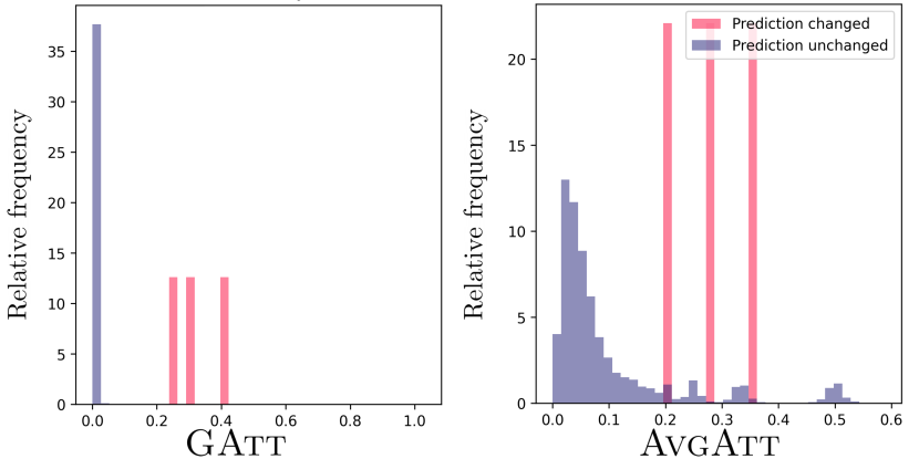
Appendix F Proof of Theorem 2.5

From the fact that the computation tree of node $w$ for an $L$ -layer GAT essentially represents the collection of all paths of length $L$ in the graph that ends with node $w$ . With this in mind, we recall the original definition of GAtt in Eq. (2):

\phi^{w}_{i,j}=\sum_{m^{\prime}=1}^{l}\sum_{\lambda_{i,j,v}^{m^{\prime}}\in\Lambda_{v}^{m^{\prime}}(e_{i,j})}C(\alpha[\lambda_{i,j,w}^{m^{\prime}}])\alpha[\lambda_{i,j,w}^{m^{\prime}}](1).

Using the double sum along with different path lengths, i.e., different values of $m$ , Eq. (2) can be rewritten as:

\phi^{w}_{i,j}=\alpha[\lambda_{i,j,w}^{1}](1)+\sum_{m^{\prime}=2}^{L}\sum_{\lambda_{i,j,w}^{m^{\prime}}\in\Lambda_{w}^{m^{\prime}}(e_{i,j})}C(\alpha[\lambda_{i,j,w}^{m^{\prime}}])\alpha[\lambda_{i,j,w}^{m^{\prime}}](1).

(14)

From the fact that $C(\alpha[\lambda_{i,j}^{m^{\prime}}])=\prod_{2\leq k\leq m^{\prime}}\alpha[\lambda_{i,j}^{m^{\prime}}](k)$ , we have $C(\alpha[\lambda_{i,j}^{m^{\prime}}])\alpha[\lambda_{i,j}^{m^{\prime}}](1)=\left(\prod_{2\leq k\leq m^{\prime}}\alpha[\lambda_{i,j}^{m^{\prime}}](k)\right)\alpha[\lambda_{i,j}^{m^{\prime}}](1)$ . Then, it follows that:

◼

$\alpha[\lambda_{i,j,w}^{m^{\prime}}](1)={\bf I}_{w,j}[\mathbf{A}(L-m^{\prime}+1)]_{j,i}$ by definition.

◼

For the argument in the second term in Eq. (14),

$\displaystyle\sum_{\lambda_{i,j,w}^{m^{\prime}}\in\Lambda_{w}^{m^{\prime}}(e_{i,j})}C(\alpha[\lambda_{i,j,w}^{m^{\prime}}])\alpha[\lambda_{i,j,w}^{m^{\prime}}](1)$	$\displaystyle=\left(\sum_{\lambda_{i,j,w}^{m^{\prime}}\in\Lambda_{w}^{m^{\prime}}(e_{i,j})}\prod_{2\leq k\leq m^{\prime}}\alpha[\lambda_{i,j,w}^{m^{\prime}}](k)\right)$
	$\displaystyle\times[\mathbf{A}(L-m^{\prime}+1)]_{j,i}$	(15)
	$\displaystyle=[\mathbf{A}(L)\mathbf{A}(L-1)\cdots\mathbf{A}(L-m^{\prime}+2)]_{w,j}$
	$\displaystyle\times[\mathbf{A}(L-m^{\prime}+1)]_{j,i}.$	(16)

Since the term $\left(\sum_{\lambda_{i,j,w}^{m^{\prime}}\in\Lambda_{w}(e_{i,j})}\prod_{2\leq k\leq m^{\prime}}\alpha[\lambda_{i,j,w}^{m^{\prime}}](k)\right)$ in the right-hand side of Eq. (15) represents the sum of the products of all attention weights along the paths from node $j$ to node $w$ of length $(m^{\prime}-1)$ , by replacing $m=L-m^{\prime}+1$ , we finally have

\phi^{v}_{i,j}=\sum_{m=1}^{L}[\mathbf{C}_{L}(L-m)]_{w,j}[{\bf A}(m)]_{j,i},

where

\mathbf{C}_{L}(k)=\begin{cases}{\bf I},&\text{if }k=0,\\ {\bf A}(L){\bf A}(L-1)\cdots{\bf A}(L-k+1),&\text{otherwise,}\end{cases}

which completes the proof of this theorem. ∎

Appendix G On the Potential Application of GAtt

Since Att-GNN has been widely applied as a backbone, GAtt can be seamlessly used as an effective tool of explaining the underlying model to unlock valuable insights that have been previously difficult to discover. Therefore, GAtt has the potential to be used to explain practical applications, which we briefly outline:

◼

Travel time estimation in transportation: Att-GNN has seen empirical success in travel time estimation (e.g., (Fang et al. 2020) from Baidu), and we expect the application of GAtt to such a domain so as to reveal which road pattern the model looks towards its estimation.
◼

Drug-target interaction in bioinformatics: Another exciting application where Att-GNN is often used as a backbone model lies in drug-target interaction prediction (Nguyen et al. 2021), where GAtt aims to confirm that the underlying model has learned the correct substructures for molecule representations, or even has discovered novel ones that dominantly affect the drug-target interaction.

Appendix H Further Case Studies (Figures 11–14)

We further conduct case studies for the BA-Shapes and Infection datasets by both visualizing the ground truth explanations and the edge attributions for randomly selected target nodes. Figures 11, 12, 13, and 14 show multiple examples of applying different edge attribution calculation methods on BA-Shapes and Infection for GAT and GATv2 models. In all cases, we observe a consistent trend: 1) GAtt of GAT/GATv2s attends more on edges in the ground truth explanations, 2) AvgAtt fails to identify such behaviors and its edge attributions tend to be spread over the graph, and 3) GAtt ${}_{\textsc{sim}}$ shows edge attribution patterns that lie between those of GAtt and AvgAtt. We refer to Appendix E.1 for case studies on SuperGAT.