Fairness for Image Generation with Uncertain Sensitive Attributes

Ajil Jalal Sushrut Karmalkar Jessica Hoffmann Alexandros G. Dimakis Eric Price

Abstract

This work tackles the issue of fairness in the context of generative procedures, such as image super-resolution, which entail different definitions from the standard classification setting. Moreover, while traditional group fairness definitions are typically defined with respect to specified protected groups – camouflaging the fact that these groupings are artificial and carry historical and political motivations – we emphasize that there are no ground truth identities. For instance, should South and East Asians be viewed as a single group or separate groups? Should we consider one race as a whole or further split by gender? Choosing which groups are valid and who belongs in them is an impossible dilemma and being “fair” with respect to Asians may require being “unfair” with respect to South Asians. This motivates the introduction of definitions that allow algorithms to be oblivious to the relevant groupings.

We define several intuitive notions of group fairness and study their incompatibilities and trade-offs. We show that the natural extension of demographic parity is strongly dependent on the grouping, and impossible to achieve obliviously. On the other hand, the conceptually new definition we introduce, Conditional Proportional Representation, can be achieved obliviously through Posterior Sampling. Our experiments validate our theoretical results and achieve fair image reconstruction using state-of-the-art generative models.

Algorithmic Fairness, Image Super-resolution, Generative Priors, Deep Generative Models, Langevin Dynamics, Posterior Sampling

1 Introduction

Refer to caption — Figure 1: Super-resolution reconstructions on Barack Obama and four faces from the FFHQ dataset. The top row shows original images, the second row shows what the algorithms observe: blurry measurements after downsampling by $32\times$ in each dimension. The third row shows reconstructions by PULSE, and the last row shows reconstructions by Posterior Sampling via Langevin dynamics, the algorithm we are advocating for. These faces were chosen to compare performance on various ethnicities. Please see Appendix A for images chosen at random from the dataset.

Fairness, accountability, and transparency have taken a front-row seat in the machine learning community. Numerous recent controversies have erupted over how current machine learning systems already in use can be racist (Simonite, 2018), sexist (Kay et al., 2015), homophobic (Morse, 2017), or all of the above (Moore, 2016). In a recent controversy, a low-resolution image of Barack Obama was put into PULSE, a super-resolution generative model (Menon et al., 2020b), but the resulting image was of a distinctly White man. While we generally have to be careful when identifying the race of a person that does not exist, such as the one represented by the generated image, multiple other reconstructions by PULSE strongly suggest that this algorithm contributes to the systemic bias against people of color.

Accuracy of representation as a fairness notion is a significant leap from the more traditional classification setting, in which we require some form of independence (or conditional independence) between the sensitive attributes and the algorithm prediction. In the context of image reconstruction, the output itself can be considered as having sensitive attributes, and we want the sensitive attributes of the input to match the sensitive attributes of the output – which is fundamentally different from an independence condition. This leads us to introduce and discuss new fairness definitions, specific to the field of image generation, reconstruction, denoising and super-resolution.

In light of the “White Obama” controversy (Menon et al., 2020b), it has been suggested that reconstruction algorithms are biased because the datasets are not representative of the true population distribution. While it is true that the datasets are biased (Buolamwini & Gebru, 2018; Khosla et al., 2012), current algorithms also play their part in widening this gap (Wang et al., 2019; Terhörst et al., 2020), such that majority classes get overrepresented, and minorities get further underrepresented. Indeed, when applying PULSE (Menon et al., 2020b) to an unbalanced dataset with 80% dogs (majority class) and 20% cats, we observe that 80% of cats are mistakenly reconstructed as dogs, while only 2% of dogs are reconstructed as cats (see Figure 4(a)). When cats are the 80% majority, the situation reverses to 1% and 98% mistakes, respectively (see Figure 5(a)).

There is a simple intuitive reason why reconstruction algorithms designed to maximize accuracy will increase bias. Assume we observe a noisy version $y$ of an image $x^{*}$ that is either a dog or a cat. Assume cats are the minority, with the prior $\Pr(x^{*}\in\text{Dog})=0.8$ . Further, assume that the measurements are always noisy and cannot definitively identify the species, so cat-like measurements are such that $p(y\mid x^{*}\in\text{Cat})/p(y\mid x^{*}\in\text{Dog})\leq 2$ . Using Bayes, the posterior is

	$\displaystyle\Pr(x^{*}\in\text{Dog}\mid y)$	$\displaystyle=p(y\mid x^{}\in\text{Dog})\cdot\frac{\Pr(x^{}\in\text{Dog})}{p(y)}$
		$\displaystyle\geq 1\cdot\frac{0.8}{0.8\cdot 1+0.2\cdot 2}$
		$\displaystyle=2/3.$

Therefore, regardless of the measurement, an algorithm that maximizes accuracy will always produce images of dogs.

This issue relates to a rich area of work on fairness in machine learning, including for classification or generation without measurements (see Section 1.1 for an overview). However, to the best of our knowledge, previous approaches always assume that the sensitive attributes are well-defined and unambiguous. While this assumption might hold for cats and dogs, as (Benthall & Haynes, 2019; Hanna et al., 2020) emphasize, race cannot be treated in the same way. First, it is unclear when to include subgroups within the larger group or when to treat them separately (for instance, when to consider South Asians as their own subgroup, or as Asians). This has major implications, as choosing which groups exist and what sensitive attributes are valid can already widen existing discrimination, as the long line of research on intersectionality shows. Second, even if we could decide on which groups are relevant, races are multidimensional and cannot be reduced to a simple categorical value: studies show that we can arrive at inconsistent conclusions about the same data depending on how race is measured (e.g. self-reported or observed) (Howell & Emerson, 2017). Our work therefore focuses on moving away from classifying people into partitions.

Problem Setting.

Suppose that we have a distribution of users $x^{*}$ ; each user $x^{*}$ is observed through some lossy observation process to produce $y$ (e.g., a low-resolution image); and our reconstruction algorithm produces $\widehat{x}$ from $y$ . We are concerned about fairness with respect to a collection of protected groups $C=\{c_{1},\dotsc,c_{k}\}$ . Our setting therefore includes, but is not limited to, the special case in which $C$ is a partition¹¹1For simplicity of notation, each group $c_{i}$ contains both people $x^{*}$ and images $\widehat{x}$ ..

The fairness concern we consider is that of representation: when users in each protected group use the algorithm, does the result adequately represent them and their group? When the observation process $y$ is significantly lossy, there inevitably will be “representation errors” where a member of one group is reconstructed as being in a different group. How should we determine if the errors are equitable?

Our Contributions: Fairness Definitions.

Figure 2: CPR, SPE and PR are achievable obliviously by Posterior Sampling. However, RDP cannot be achieved obliviously, and if a majority group exists it cannot be achieved simultaneously with PR.

We introduce definitions for some natural notions of fairness in reconstruction. One is that the average representation rate should be independent of the group:

\displaystyle\Pr(\widehat{x}\in c_{i}\mid x^{*}\in c_{i})

(RDP)

is the same value for all $i\in[k]$ . We call this Representation Demographic Parity (RDP), by analogy to the binary classification setting, where Demographic Parity means that $\Pr(L=1\mid x^{*}\in c_{i})$ is fixed. The difference here is that the “good” outcome $(\widehat{x}\in c_{i})$ is different for each group, while typically in classification the “good” outcome (where, e.g., $L=1$ means “offer a loan”) is the same across groups. RDP is simply requesting that the reconstructions have the same error rates across groups.

An alternative definition is that the demographics of the output should match those of the input:

\displaystyle\Pr(\widehat{x}\in c_{i})=\Pr(x^{*}\in c_{i})~{}~{}\forall i.

(PR)

We call this Proportional Representation (PR). It simply says that the reconstruction process should not introduce bias in the distribution for or against any group.

Unfortunately, these two definitions are often incompatible. We show in Proposition 2.8 that, whenever a majority group exists and the measurements can confuse it with other groups, no algorithm can achieve both RDP and PR.

One weakness of both PR and RDP is that they only consider the global behavior of the reconstruction. But individual users want to be represented well when they use the system, and may not be mollified by the knowledge that many other members of their group are being represented. On the other hand, some images are genuinely harder to reconstruct accurately, so expecting equal representation accuracy/RDP for every user would strongly limit overall accuracy. Our solution is to extend PR by incorporating the measurement process:

\displaystyle\Pr(\widehat{x}\in c_{i}\mid y)=\Pr(x^{*}\in c_{i}\mid y)~{}~{}\forall i,y.

(CPR)

We call this Conditional Proportional Representation (CPR). The idea is that the population of users with each given $y$ should have fair treatment (in the sense of PR). Of course, CPR implies PR by averaging over $y$ .

Note that CPR implies that the reconstruction process must be randomized, not deterministic. This has other benefits: if the user is not satisfied with the result, they can rerun the algorithm until they get a result that represents them. Users can also get a collection of $\widehat{x}_{i}$ to observe the diversity of possible reconstructions.

Our Contributions: Algorithms.

We show that CPR (and hence PR) are achievable with a simple-to-describe algorithm: posterior sampling, where we output $\widehat{x}\sim p(x^{*}\mid y)$ . This can be approximated well in practice using Langevin dynamics for state-of-the-art generative models representing $p(x^{*})$ , as we discuss in Section 4.1.

Posterior Sampling also satisfies one more fairness condition: the confusion matrix is symmetric, meaning that (for example) an equal number of Black users will be reconstructed as White as White users will be reconstructed as Black. We call this condition Symmetric Pairwise Error (SPE).

\displaystyle\Pr\left(\widehat{x}\in c_{i},x^{*}\in c_{j}\right)=\Pr\left(\widehat{x}\in c_{j},x^{*}\in c_{i}\right).

(SPE)

for all $i,j\in[k]$ . CPR implies SPE, and SPE implies PR (see Figure 2).

Since SPE implies PR, in general SPE is incompatible with RDP (per Proposition 2.8). But in the special case of two groups $c_{1},c_{2}$ of equal size, then SPE actually implies RDP. This gives an algorithm to achieve RDP for the two-group setting: we reweight our input distribution such that each group has equal probability, then perform Posterior Sampling with respect to the reweighted distribution. With more than two groups, there still exists a reweighting of the groups such that Posterior Sampling on the reweighted distribution satisfies RDP (see Theorem 3.5). This reweighted-resampling algorithm can be performed in practice by learning a GAN for the reweighted distribution and using Langevin dynamics on the reweighted GAN.

Our Contributions: Obliviousness.

Posterior Sampling satisfies the CPR, PR, and SPE fairness criteria while retaining an invaluable property: the algorithm doesn’t depend on the set of protected groups $C$ . It satisfies the fairness properties for every set of protected groups, which is an algorithmically achievable way of addressing the issues raised in (Hanna et al., 2020) about race being ambiguous and ill-defined. We say such an algorithm is obliviously fair. By contrast, our reweighted-resampling algorithm achieving RDP needs to know the protected groups, and would not satisfy RDP for a different collection of groups. Which fairness properties can be achieved obliviously, and under what circumstances?

Our main results here are twofold: first, Posterior Sampling is the only algorithm that satisfies CPR obliviously. Second, RDP cannot be satisfied obliviously. This impossibility applies even to obliviousness with respect to one of two plausible, socially meaningful partitions. Theorem 2.4 shows, for example, that you cannot satisfy RDP with respect to both {White, Asian} and {White, South Asian, East Asian} if your observations are lossy. This means that every algorithm can reasonably be viewed as unfair with respect to RDP.

Our Contributions: Experiments.

We implement Posterior Sampling via Langevin dynamics, study its empirical performance and compare it to PULSE with respect to our defined metrics. We do this on the MNIST (LeCun, 1998), FlickrFaces-HQ (Karras et al., 2019) and AFHQ cat & dog (Choi et al., 2020b) datasets. We evaluate obliviousness and SPE of Posterior Sampling on the first two datasets. Using the AFHQ cat & dog dataset, we demonstrate empirically that Posterior Sampling satisfies SPE and PR over various imbalances between cats and dogs.

1.1 Related Work

Numerous works have attempted to tackle the issue of bias in the machine learning of images, either for data generation/reconstruction tasks or for downstream tasks such as face recognition and image quality assessment. One popular approach for dealing with bias consists of adversarially generating data or embeddings with a discriminator for different values of the sensitive attributes, yielding similar distributions for different values of the sensitive attribute (Madras et al., 2018; Xu et al., 2018, 2019; Gong et al., 2020a; Khajehnejad et al., ; Sattigeri et al., 2018; Yu et al., 2020). Another approach focuses on learning explicitly the bias of the dataset, so as to remove it (Khosla et al., 2012; Grover et al., 2019; Choi et al., 2020a). The special case of fair dimensionality reduction through principal component analysis is solved by (Samadi et al., 2018). Another research direction formulates the fairness constraints as an additional term in the loss (Serna et al., 2020). Another approach focuses on minorities and learns their specific features (Amini et al., 2019; Gong et al., 2020b). A related line of work improves the fairness of generative models without retraining (Tan et al., 2020), however we do not know how to use these for inverse problems.

Another relevant line of research studies fairness in the presence of uncertainty, either in the labels (Kleinberg & Raghavan, 2018; Blum & Stangl, 2019; Wang et al., 2020a; Rolf et al., 2020) or in the sensitive attributes (Awasthi et al., 2020; Lamy et al., 2019; Celis et al., 2020; Wang et al., 2020b). In particular, one work studies overlapping groups (Yang et al., 2020).

Super resolution using deep learning has had remarkable success at producing accurate images. In (Ledig et al., 2017), the authors provide an algorithm which performs photo-realistic super resolution using GANs. However, this model requires retraining of the GAN when the measurement operator changes. Subsequent work has overcome this hurdle. Some models independent of the forward operator include CSGM (Bora et al., 2017), OneNet (Chang et al., 2017), PULSE (Menon et al., 2020a), Deep Image Prior (Ulyanov et al., 2018) and Deep Decoder (Heckel et al., 2019). Another line of work has shown that Posterior Sampling using approximate deep generative priors is instance-optimal for compressed sensing (Jalal et al., 2021).

2 Fairness definitions for image generation

2.1 Representation Demographic Parity

While multiple group fairness definitions (demographic parity, equalized odds or opportunity, calibration etc.(Barocas et al., 2017; Hardt et al., 2016)) have been studied and widely accepted in the context of classification, their extension to the setting of image generation is not immediate. Here, we extend demographic parity.

Definition 2.1.

Let $x^{*}\in\mathbb{R}^{n}$ denote the ground truth, and $P$ denote its distribution. Let $y\in\mathbb{R}^{m}$ be some measurements of $x^{*}$ . For a collection $C=\{c_{1},\dots,c_{k}\}$ of (potentially overlapping) sets, an algorithm which reconstructs $x^{*}$ using $y$ satisfies Representation Demographic Parity (RDP) if:

\forall i,j\in[k],\,\,\Pr(\hat{x}\in c_{i}|x^{*}\in c_{i})=\Pr(\hat{x}\in c_{j}|x^{*}\in c_{j}).

Example 2.2.

If $k=2$ , $c_{1}$ being all women, $c_{2}$ being all non-women, Representation Demographic Parity with respect to these two groups implies that women are as likely to be reconstructed as women as non-women are to be reconstructed as non-women.

2.2 Limitations of traditional group fairness definitions

Inspired by (Hanna et al., 2020), we note several reasons for having fairness definitions that are more flexible with respect to the groups in the collection or partition.

Minorities are ill-defined: What constitutes a minority? Are South Asians their own subgroup, or are they assigned as Asians? The list of accepted minorities is not only inconsistent across location and purpose, but multiple levels of granularity could be equally valid. Similar concerns can be raised from the point of view of intersectionality: we might both be interested in the discrimination faced by all women, and all people of color, without wanting to erase the singular discrimination faced by women of color (Buolamwini & Gebru, 2018).

Races are multi-dimensional: As (Roth, 2016) argues, races are multi-dimensional, and these dimensions are all relevant, albeit in different settings. For instance, voting patterns are more accurately predicted based on self-identified race, while observed race is more informative when dealing with discrimination. These differences are not minor: as (Howell & Emerson, 2017) shows, measuring races in five different ways led to widely different interpretations of the same data.

Partitions reify the status quo: According to (Hanna et al., 2020), widespread adoption of race categories participates in erasing their historical and social context (Duster, 2005; Smart et al., 2008), as well as perpetuating the current system and creating new harm (Kaufman, 1999; Sewell, 2016).

Who chooses the partition: (Barabas et al., 2020) raises concerns on who has the power to choose the partitions and what their intentions were. Historically, such partitions have done significant harm to the minorities they were supposed to protect (Mills, 2014; Hanna et al., 2020).

In response to these critiques, we study a novel property of fairness definitions.

Definition 2.3 (obliviously).

We say an algorithm satisfies a group fairness definition obliviously if the algorithm satisfies the fairness definition for any collection of sets and does not require knowledge of the collection of sets to perform reconstruction.

Satisfying a fairness definition obliviously is one way of addressing the issues above, as it is now satisfied for all groups at the same time. This requirement may nevertheless be too strong, since most such groupings are not socially meaningful. This leads to more restricted versions of obliviousness, ones that only hold for specific sets of collections. Unfortunately, RDP cannot be satisfied even with only two socially meaningful partitions.

Theorem 2.4.

Let $A$ and $B$ be disjoint groups (e.g., Asian and White people), and let $A_{1},A_{2}\subset A$ be disjoint groups that cannot be perfectly distinguished from measurements only (e.g., South Asians and East Asians). Then Representation Demographic Parity cannot be satisfied $\{\{A,B\},\,\{A_{1},A_{2},B\}\}$ -obliviously.

In the example stated in Theorem 2.4, it is impossible to be fair as defined by Representation Demographic Parity with respect to White people, South Asians, East Asians, and Asians as a whole. This holds even if we know exactly what the measurement process is, the demographics, and what the relevant groups are.

We can state this more generally:

Theorem 2.5 (Representation Demographic Parity cannot be satisfied obliviously).

The only way for an algorithm to satisfy Representation Demographic Parity obliviously is to achieve perfect reconstruction.

2.3 Conditional Proportional Representation

An alternative fairness measure is that the distribution of the output of the algorithm should match the demographics of the input to the algorithm:

Definition 2.6 (Proportional Representation).

In the setting of Definition 2.1, an algorithm satisfies Proportional Representation (PR) if:

\displaystyle\forall i\in\left[k\right],\;\Pr\left(\widehat{x}\in c_{i}\right)=\Pr\left(x^{*}\in c_{i}\right).

One could also demand a much stricter fairness property, where the algorithm should satisfy PR among the population that maps to the same observation, for every possible observation:

Definition 2.7 (Conditional Proportional Representation).

In the setting of Definition 2.1, an algorithm satisfies Conditional Proportional Representation (CPR) if, almost surely over $y$ :

\displaystyle\forall i\in\left[k\right],\;\Pr\left(\widehat{x}\in c_{i}|y\right)=\Pr\left(x^{*}\in c_{i}|y\right).

Intuitively, many images could yield the same lossy measurement. Because we have no way of knowing exactly from which image the measurement came, we reconstruct one at random based on how likely images in the same group are to have yielded this measurement in the first place. As such, it is “fair”: every image that could have led to the measurement gets a chance at being represented, not just the most likely. This also implies that the reconstruction cannot be deterministic. Unfortunately, while CPR can be achieved via Posterior Sampling (Theorem 3.1), the fact that the definition involves the posterior distribution makes it difficult to verify without full knowledge of the measurement process and the probability distribution.

It turns out that one cannot achieve RDP and PR simultaneously if you have a majority which has mass larger than $1/2$ .

Proposition 2.8.

Whenever there exists a majority class that the measurements cannot 100% distinguish from the non-majority classes, PR and RDP are not simultaneously achievable.

3 Posterior Sampling

The Posterior Sampling algorithm outputs a reconstruction $\widehat{x}$ drawn from the posterior $P(\cdot\mid y)$ . It is known to be instance-optimal for compressed sensing (Jalal et al., 2021) and to give fairly accurate results in practice when implemented via annealed Langevin dynamics (Song & Ermon, 2019b). In this section, we show that it also has good fairness properties.

It is easy to see that if one has access to the distribution $P$ over images and the likelihood function associated with the measurement process, then Posterior Sampling will satisfy the CPR. The following Theorem shows that this is the only algorithm that can satisfy CPR.

Theorem 3.1.

Posterior Sampling is the only algorithm that achieves oblivious Conditional Proportional Representation.

Definition 3.2 (Symmetric Pairwise Error).

In the setting of Definition 2.1, an algorithm satisfies Symmetric Pairwise Error (SPE) if

\displaystyle\Pr\left(\widehat{x}\in c_{i},x^{*}\in c_{j}\right)=\Pr\left(\widehat{x}\in c_{j},x^{*}\in c_{i}\right),\;\forall i,j\in\left[k\right].

Using the fact that the ground truth and reconstruction are conditionally independent given the measurements, we can show that any algorithm that satisfies CPR will also satisfy SPE.

Theorem 3.3.

In the setting of Definition 2.1, Conditional Proportional Representation implies Symmetric Pairwise Error.

Theorem 3.1 and Theorem 3.3 give the following Corollary.

Corollary 3.4.

Posterior Sampling achieves symmetric pairwise error for any pair of sets $U,V\subset\mathbb{R}^{n}$ .

Finally, for any partition $C$ , there exists a reweighting of the underlying distribution such that Posterior Sampling achieves RDP with respect to the partition $C$ .

Theorem 3.5.

Let $C=\{c_{1},\dots,c_{k}\}$ be a partition. There exists a choice of weights $\lambda_{i}>0$ with $\sum\lambda_{i}=1$ such that Posterior Sampling with respect to the reweighted distribution

p_{\lambda}(x)=\sum_{i}\lambda_{i}p(x\mid x\in c_{i})

satisfies RDP with respect to $C$ .

In the special case of 2 classes, the reweighting is very simple: $\lambda_{1}=\lambda_{2}=\frac{1}{2}$ .

3.1 Representation Cross-Entropy

For the special case when the collection $C$ is a partition, we can show that Posterior Sampling obliviously minimizes a loss we call Representation Cross-Entropy (RCE). Intuitively, one can think of this as the generative analogue of the cross-entropy loss popular in classification settings. Following the notation in Definition 2.1, we define RCE as:

Definition 3.6 (Representation Cross-Entropy).

Let $C=\left\{c_{1},\cdots,c_{k}\right\}$ form a disjoint partition of $\mathbb{R}^{n}$ , and let $U$ be a function such that $U(x)$ encodes where $x$ lies in the partition. The Representation Cross-Entropy (RCE) of a reconstruction algorithm $\mathcal{A}$ with respect to $C$ is defined as

\displaystyle RCE(\mathcal{A}):=-\operatorname*{\mathbb{E}}_{x^{*},y}\log\Pr_{\widehat{x}|y}\left[\widehat{x}\in U(x^{*})\right].

We show that if we want to minimize RCE over a partition, then we must have CPR on this partition:

Theorem 3.7.

Let $C=\left\{c_{1},\cdots,c_{k}\right\}$ form a disjoint partition of $\mathbb{R}^{n}$ . An algorithm minimizes Representation Cross-Entropy on $C$ iff the algorithm satisfies CPR on $C$ .

From Theorem 3.1, we know that Posterior Sampling is the only algorithm that can achieve CPR over all measurable sets. The same result holds if we restrict to measurable partitions, so Posterior Sampling is the only algorithm that minimizes RCE obliviously to the partition.

4 Experiments

So far we have discussed and analyzed properties of several different fairness metrics. In this section, we briefly describe how one can implement Posterior Sampling, and study the empirical performance of Posterior Sampling and PULSE with respect to our defined metrics, on the MNIST (LeCun, 1998), FlickrFaces-HQ (Karras et al., 2019) and AFHQ cat&dog dataset (Choi et al., 2020b).

4.1 Langevin Dynamics

We implement Posterior Sampling via Langevin dynamics, which states that if $x_{0}\sim\mathcal{N}(0,cI_{n}),$ (for $c$ appropriately small), then we can sample from $p(x|y)$ by running noisy gradient ascent:

\displaystyle x_{t+1}\leftarrow x_{t}+\gamma_{t}\nabla_{x_{t}}\log p(x_{t}|y)+\sqrt{2\gamma_{t}}\xi_{t},

where $\xi_{t}\sim\mathcal{N}(0,I_{n})$ is an i.i.d. standard Gaussian drawn at each iteration. It is well known (Welling & Teh, 2011; Song & Ermon, 2019b) that as $\gamma_{t}\to 0,t\to\infty,$ we have $p(x_{t}|y)\to p(x|y).$ In practice, we need some form of annealing of the noise in order to mix efficiently. Since our algorithm is randomized, we always output the first obtained reconstruction. Please see Appendix D for architecture-specific details.

4.2 MNIST dataset

We trained a VAE (Kingma & Welling, 2013) on MNIST digits, and consider the groups {0, 1, 2, 3, 4, $\geq 5$ }. As seen in the confusion matrix in Table 1, Posterior Sampling does satisfy SPE obliviously over the groups (recall that SPE also implies PR).

	0	1	2	3	4	$\geq 5$
0	33	2	0	2	0	6
1	0	61	1	0	1	4
2	0	2	45	1	1	6
3	1	0	2	33	2	7
4	1	0	1	0	41	12
$\geq 5$	2	5	10	5	14	199

Table 1: Confusion matrix for super-resolution of MNIST digits after downsampling by

4\times

in each dimension. The rows denote the labels of original images, the columns denote the labels of reconstructed images. The symmetric nature of the matrix shows that Posterior Sampling achieves SPE obliviously over multiple groups.

4.3 FlickrFaces dataset

Dataset and generative models.

We use a StyleGAN2 (Karras et al., 2020b) model for PULSE, while Posterior Sampling uses the NCSNv2 generative model (Song & Ermon, 2019a, 2020). We choose this model as it has been designed to produce images via Langevin dynamics, which is the practical implementation of Posterior Sampling.

Results

In Figure 1, we show the results of super-resolution on Barack Obama and four faces from FFHQ, using PULSE and Posterior Sampling. As shown, Posterior Sampling preserves the image features better than PULSE. We use the CLIP classifier (Radford et al., 2021) to assign labels of {child with / without glasses, adult with / without glasses}, and report the confusion matrix in Table 2. This shows that Posterior Sampling satisfies SPE over multiple groups obliviously.

Please see Appendix A for more representative samples. These correspond to images 69000-69020 in the FFHQ validation set (these were the first 20 images as we downloaded them in reverse-chronological order from the Google Drive folder).

	A	B	C	D
A	5	3	2	0
B	1	99	0	10
C	1	0	68	10
D	1	10	8	282

Table 2: Confusion matrix for super-resolution of FFHQ faces after

32\times

downsampling in each dimension. The categories are A: child with glasses, B: child without glasses, C: adult with glasses, D: adult without glasses. Rows denote labels of original images, columns denote labels of reconstructed images. The symmetric nature of the matrix shows that Posterior Sampling achieves SPE over multiple groups obliviously.

4.4 AFHQ Cats and Dogs dataset

Dataset and models

We trained StyleGAN2 (Karras et al., 2020a) on the AFHQ cat & dog (Choi et al., 2020b) training set. In order to study the effect of population bias on PULSE and Posterior Sampling, we trained three models on datasets with varying bias: (1) 20% cats and 80% dogs, (2) 80% cats and 20% dogs, and (3) 50% cats and 50% dogs.

In order to label the images generated by the GAN, we take a pre-trained Resnet108 and retrain the last layer using labelled images from the AFHQ training set. We find that the classifier’s predictions does match the human perception of dogs and cats in general.

Posterior Sampling satisfies SPE and PR when the cats and dogs are unbalanced.

For this experiment, we draw $x^{*}$ from the AFHQ validation dataset, which contains 500 images of cats and 500 images of dogs. Since we want to study whether Posterior Sampling and PULSE satisfy SPE and PR, we construct the test set to match the training population of the generator. That is, for the 20% cat generator, we use 125 images of cats and all 500 images of dogs from the AFHQ dataset. Similarly, for the 80% cat generator, we use 500 images of cats and 125 images of dogs in the test set.

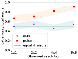
We then downscale the images, and vary the downscaling factor such that the observed measurements have resolution $1\times 1,2\times 2,4\times 4,8\times 8.$ We ran PULSE and Posterior Sampling to super-resolve the blurry measurements, and used a classifier to count how many cats and dogs were reconstructed in the wrong class. The results for the 20% cat generator are in Table 3(a) and Figure 4(a), and the results for the 80% cat generator are in Table 4(a) and Figure 5(a). In Figure 3 we show example reconstructions.

We find that PULSE consistently makes very few mistakes on the majority, and an overwhelming number of mistakes on the minority. Posterior Sampling, however, makes an approximately equal number of mistakes on each class (i.e., satisfies SPE). Equivalently for this 2-class setting, it generates cats and dogs in proportion to their population (i.e., satisfies PR).

$m$	PULSE	Ours
$1\times 1$	113	58	102	106
$2\times 2$	104	44	97	81
$4\times 4$	110	25	94	110
$8\times 8$	101	10	70	59

$m$	PULSE	Ours
$1\times 1$	0	125	115	96
$2\times 2$	0	125	82	97
$4\times 4$	0	125	94	86
$8\times 8$	1	123	71	94

Posterior Sampling satisfies RDP, SPE, and PR when the cats and dogs are balanced.

We use a generator trained on 50% cats and 50% dogs, and study whether Posterior Sampling and PULSE satisfy RDP, SPE, and PR in practice. In this case, we use all images of cats and dogs from the AFHQ validation set. These results are in Appendix B, Figure 10. Please see Appendix B for more results as we vary the training bias of the generator and test SPE for images drawn from the range of the generator.

5 Limitations

The fact that CPR can be satisfied obliviously is its main strength, as the subgroups one would like to protect are often not well defined or labeled in datasets. This is especially beneficial for overlooked groups that lack the power to convince an algorithm designer to cater to them. However, obliviousness can also be seen as a weakness, as it leads to symmetry in the number of errors in each group rather than the fraction of errors. For two groups, this means that the minority group will always have higher error rate than the majority.

Furthermore, the goal of CPR is to treat the members of each group equally. The philosophical stance behind this property implicitly views being “fair” as treating individuals equally, and hence representing groups in proportion to their size. However, alternative philosophical stances exist. In particular, it is at odds with the idea that historically oppressed minorities should get particular attention (Hanna et al., 2020). One could adapt such an approach into our framework by reweighting the classes, analogous to Theorem 3.5, but doing so requires explicit group information.

Finally, all of the definitions we consider focus on representation but do not consider the quality of the reconstruction. If all reconstructions on minorities were of poor quality (for instance because the training set did not have enough images of this specific minority, and/or they were of poorer quality, as we know can happen (Buolamwini & Gebru, 2018)), the algorithm could still satisfy any of the definitions and be deemed “fair” according to it. Representation fairness is just one piece of the larger question of fairness in reconstruction.

6 Conclusion

In the image generation setting, fairness is related to the concept of representation: we assign a protected group to the output, which should match the protected group of the input. This is a stark contrast with the classification setting, in which we usually require some form of independence between the output and the sensitive attributes. We therefore introduce two notions of fairness, an extension of demographic parity called Representation Demographic Parity (RDP), and a conceptually new notion, Conditional Proportional Representation (CPR). We show that these notions are in general incompatible. Furthermore, we prove that RDP is strongly dependent on the choice of the protected groups. This is especially problematic for generating images of people, as races are usually ill-defined and/or ambiguous. CPR, however, does not suffer from these downsides, and can even be satisfied obliviously (i.e., simultaneously for any choice of protected groups).

We prove that Posterior Sampling can achieve CPR, and is actually the only algorithm that can achieve CPR fully obliviously. We show how to experimentally implement our findings through Langevin dynamics, and our experiments exhibit the expected desirable properties.

We see our work as a first step towards better understanding ideas of fairness in the context of generating structured data – our paper deals with image generation, but the problem of generating structured data could be extended to other settings. What happens when the data is of a different type? For instance, one might want to predict pronouns in the context of text completion or generation, or provide the option to use a certain dialect.

The definitions introduced in this paper are specific to generative procedures. However, the underlying issues – having definitions that do not strongly rely on the choice of the protected groups – can be found in the classification setting as well. It would be interesting to see if any analogs of CPR exist in this more traditional setting, and if there exist algorithms that can achieve it obliviously.

7 Acknowledgements

Ajil Jalal and Alex Dimakis were supported by NSF Grants CCF 1934932, AF 1901292, 2008710, 2019844 the NSF IFML 2019844 award and research gifts by Western Digital, WNCG and MLL, computing resources from TACC and the Archie Straiton Fellowship. Sushrut Karmalkar was supported by a University Graduate Fellowship from the University of Texas at Austin. Jessica Hoffmann was supported by NSF TRIPODS grant 1934932. Eric Price was supported by NSF Award CCF-1751040 (CAREER) and NSF IFML 2019844.

References

Amini et al. (2019) Amini, A., Soleimany, A. P., Schwarting, W., Bhatia, S. N., and Rus, D. Uncovering and mitigating algorithmic bias through learned latent structure. In Proceedings of the 2019 AAAI/ACM Conference on AI, Ethics, and Society, pp. 289–295, 2019.
Awasthi et al. (2020) Awasthi, P., Kleindessner, M., and Morgenstern, J. Equalized odds postprocessing under imperfect group information. In International Conference on Artificial Intelligence and Statistics, pp. 1770–1780. PMLR, 2020.
Barabas et al. (2020) Barabas, C., Doyle, C., Rubinovitz, J., and Dinakar, K. Studying up: reorienting the study of algorithmic fairness around issues of power. In Proceedings of the 2020 Conference on Fairness, Accountability, and Transparency, pp. 167–176, 2020.
Barocas et al. (2017) Barocas, S., Hardt, M., and Narayanan, A. Fairness in machine learning. Nips tutorial, 1:2, 2017.
Benthall & Haynes (2019) Benthall, S. and Haynes, B. D. Racial categories in machine learning. In Proceedings of the Conference on Fairness, Accountability, and Transparency, pp. 289–298, 2019.
Blum & Stangl (2019) Blum, A. and Stangl, K. Recovering from biased data: Can fairness constraints improve accuracy? arXiv preprint arXiv:1912.01094, 2019.
Bora et al. (2017) Bora, A., Jalal, A., Price, E., and Dimakis, A. G. Compressed sensing using generative models. In International Conference on Machine Learning, pp. 537–546. PMLR, 2017.
Buolamwini & Gebru (2018) Buolamwini, J. and Gebru, T. Gender shades: Intersectional accuracy disparities in commercial gender classification. In Friedler, S. A. and Wilson, C. (eds.), Proceedings of the 1st Conference on Fairness, Accountability and Transparency, volume 81 of Proceedings of Machine Learning Research, pp. 77–91, New York, NY, USA, 23–24 Feb 2018. PMLR. URL http://proceedings.mlr.press/v81/buolamwini18a.html.
Celis et al. (2020) Celis, L. E., Huang, L., and Vishnoi, N. K. Fair classification with noisy protected attributes. arXiv preprint arXiv:2006.04778, 2020.
Chang et al. (2017) Chang, R. J., Li, C.-L., Poczos, B., Vijaya Kumar, B., and Sankaranarayanan, A. C. One network to solve them all–solving linear inverse problems using deep projection models. In Proceedings of the IEEE International Conference on Computer Vision, pp. 5888–5897, 2017.
Choi et al. (2020a) Choi, K., Grover, A., Singh, T., Shu, R., and Ermon, S. Fair generative modeling via weak supervision. In International Conference on Machine Learning, pp. 1887–1898. PMLR, 2020a.
Choi et al. (2020b) Choi, Y., Uh, Y., Yoo, J., and Ha, J.-W. Stargan v2: Diverse image synthesis for multiple domains. In Proceedings of the IEEE/CVF Conference on Computer Vision and Pattern Recognition, pp. 8188–8197, 2020b.
Duster (2005) Duster, T. Race and reification in science, 2005.
Gong et al. (2020a) Gong, S., Liu, X., and Jain, A. K. Jointly de-biasing face recognition and demographic attribute estimation. In European Conference on Computer Vision, pp. 330–347. Springer, 2020a.
Gong et al. (2020b) Gong, S., Liu, X., and Jain, A. K. Mitigating face recognition bias via group adaptive classifier. arXiv preprint arXiv:2006.07576, 2020b.
Grover et al. (2019) Grover, A., Choi, K., Shu, R., and Ermon, S. Fair generative modeling via weak supervision. 2019.
Hanna et al. (2020) Hanna, A., Denton, E., Smart, A., and Smith-Loud, J. Towards a critical race methodology in algorithmic fairness. In Proceedings of the 2020 Conference on Fairness, Accountability, and Transparency, pp. 501–512, 2020.
Hardt et al. (2016) Hardt, M., Price, E., and Srebro, N. Equality of opportunity in supervised learning. In Proceedings of the 30th International Conference on Neural Information Processing Systems, NIPS’16, pp. 3323–3331, Red Hook, NY, USA, 2016. Curran Associates Inc. ISBN 9781510838819.
Heckel et al. (2019) Heckel, R. et al. Deep decoder: Concise image representations from untrained non-convolutional networks. In International Conference on Learning Representations, 2019.
Howell & Emerson (2017) Howell, J. and Emerson, M. O. So what “should” we use? evaluating the impact of five racial measures on markers of social inequality. Sociology of Race and Ethnicity, 3(1):14–30, 2017. doi: 10.1177/2332649216648465. URL https://doi.org/10.1177/2332649216648465.
Jalal et al. (2021) Jalal, A., Karmalkar, S., Dimakis, A. G., and Price, E. Instance-optimal compressed sensing via posterior sampling. arXiv preprint arXiv:2106.11438, 2021.
Karras et al. (2019) Karras, T., Laine, S., and Aila, T. A style-based generator architecture for generative adversarial networks. In Proceedings of the IEEE/CVF Conference on Computer Vision and Pattern Recognition, pp. 4401–4410, 2019.
Karras et al. (2020a) Karras, T., Aittala, M., Hellsten, J., Laine, S., Lehtinen, J., and Aila, T. Training generative adversarial networks with limited data. arXiv preprint arXiv:2006.06676, 2020a.
Karras et al. (2020b) Karras, T., Laine, S., Aittala, M., Hellsten, J., Lehtinen, J., and Aila, T. Analyzing and improving the image quality of stylegan. In Proceedings of the IEEE/CVF Conference on Computer Vision and Pattern Recognition, pp. 8110–8119, 2020b.
Kaufman (1999) Kaufman, J. S. How inconsistencies in racial classification demystify the race construct in public health statistics. Epidemiology, pp. 101–103, 1999.
Kay et al. (2015) Kay, M., Matuszek, C., and Munson, S. A. Unequal representation and gender stereotypes in image search results for occupations. In Proceedings of the 33rd Annual ACM Conference on Human Factors in Computing Systems, pp. 3819–3828, 2015.
(27) Khajehnejad, M., Rezaei, A. A., Babaei, M., Hoffmann, J., Jalili, M., and Weller, A. Adversarial graph embeddings for fair influence maximization over social networks.
Khosla et al. (2012) Khosla, A., Zhou, T., Malisiewicz, T., Efros, A. A., and Torralba, A. Undoing the damage of dataset bias. In European Conference on Computer Vision, pp. 158–171. Springer, 2012.
Kingma & Welling (2013) Kingma, D. P. and Welling, M. Auto-encoding variational bayes. arXiv preprint arXiv:1312.6114, 2013.
Kleinberg & Raghavan (2018) Kleinberg, J. and Raghavan, M. Selection problems in the presence of implicit bias. arXiv preprint arXiv:1801.03533, 2018.
Lamy et al. (2019) Lamy, A. L., Zhong, Z., Menon, A. K., and Verma, N. Noise-tolerant fair classification. arXiv preprint arXiv:1901.10837, 2019.
LeCun (1998) LeCun, Y. The mnist database of handwritten digits. http://yann. lecun. com/exdb/mnist/, 1998.
Ledig et al. (2017) Ledig, C., Theis, L., Huszár, F., Caballero, J., Cunningham, A., Acosta, A., Aitken, A., Tejani, A., Totz, J., Wang, Z., et al. Photo-realistic single image super-resolution using a generative adversarial network. In Proceedings of the IEEE conference on computer vision and pattern recognition, pp. 4681–4690, 2017.
Madras et al. (2018) Madras, D., Creager, E., Pitassi, T., and Zemel, R. Learning adversarially fair and transferable representations. arXiv preprint arXiv:1802.06309, 2018.
Menon et al. (2020a) Menon, S., Damian, A., Hu, S., Ravi, N., and Rudin, C. Pulse: Self-supervised photo upsampling via latent space exploration of generative models. In Proceedings of the IEEE/CVF Conference on Computer Vision and Pattern Recognition, pp. 2437–2445, 2020a.
Menon et al. (2020b) Menon, S., Damian, A., Hu, S., Ravi, N., and Rudin, C. Pulse: Self-supervised photo upsampling via latent space exploration of generative models. 2020 IEEE/CVF Conference on Computer Vision and Pattern Recognition (CVPR), 2020b. doi: 10.1109/cvpr42600.2020.00251. URL http://dx.doi.org/10.1109/cvpr42600.2020.00251.
Mills (2014) Mills, C. W. The racial contract. Cornell University Press, 2014.
Moore (2016) Moore, M. Microsoft deletes ai chatbot after racist, homophobic tweets, according to report. SD Times, March, 2016.
Morse (2017) Morse, J. Google’s ai has some seriously messed up opinions about homosexuality. Mashable, October, 2017.
Radford et al. (2021) Radford, A., Kim, J. W., Hallacy, C., Ramesh, A., Goh, G., Agarwal, S., Sastry, G., Askell, A., Mishkin, P., Clark, J., et al. Learning transferable visual models from natural language supervision. arXiv preprint arXiv:2103.00020, 2021.
Rolf et al. (2020) Rolf, E., Simchowitz, M., Dean, S., Liu, L. T., Bjorkegren, D., Hardt, M., and Blumenstock, J. Balancing competing objectives with noisy data: Score-based classifiers for welfare-aware machine learning. In International Conference on Machine Learning, pp. 8158–8168. PMLR, 2020.
Roth (2016) Roth, W. D. The multiple dimensions of race. Ethnic and Racial Studies, 39(8):1310–1338, 2016.
Samadi et al. (2018) Samadi, S., Tantipongpipat, U., Morgenstern, J. H., Singh, M., and Vempala, S. The price of fair pca: One extra dimension. In Advances in neural information processing systems, pp. 10976–10987, 2018.
Sattigeri et al. (2018) Sattigeri, P., Hoffman, S. C., Chenthamarakshan, V., and Varshney, K. R. Fairness gan. arXiv preprint arXiv:1805.09910, 2018.
Serna et al. (2020) Serna, I., Morales, A., Fierrez, J., Cebrian, M., Obradovich, N., and Rahwan, I. Sensitiveloss: Improving accuracy and fairness of face representations with discrimination-aware deep learning. arXiv preprint arXiv:2004.11246, 2020.
Sewell (2016) Sewell, A. A. The racism-race reification process: A mesolevel political economic framework for understanding racial health disparities. Sociology of Race and Ethnicity, 2(4):402–432, 2016.
Simonite (2018) Simonite, T. When it comes to gorillas, google photos remains blind. Wired, January, 11, 2018.
Smart et al. (2008) Smart, A., Tutton, R., Martin, P., Ellison, G. T., and Ashcroft, R. The standardization of race and ethnicity in biomedical science editorials and uk biobanks. Social Studies of Science, 38(3):407–423, 2008.
Song & Ermon (2019a) Song, Y. and Ermon, S. Generative modeling by estimating gradients of the data distribution. In Advances in Neural Information Processing Systems, pp. 11895–11907, 2019a.
Song & Ermon (2019b) Song, Y. and Ermon, S. Generative modeling by estimating gradients of the data distribution. In Wallach, H., Larochelle, H., Beygelzimer, A., d'Alché-Buc, F., Fox, E., and Garnett, R. (eds.), Advances in Neural Information Processing Systems, volume 32, pp. 11918–11930. Curran Associates, Inc., 2019b. URL https://proceedings.neurips.cc/paper/2019/file/3001ef257407d5a371a96dcd947c7d93-Paper.pdf.
Song & Ermon (2020) Song, Y. and Ermon, S. Improved techniques for training score-based generative models. arXiv preprint arXiv:2006.09011, 2020.
Tan et al. (2020) Tan, S., Shen, Y., and Zhou, B. Improving the fairness of deep generative models without retraining. arXiv preprint arXiv:2012.04842, 2020.
Terhörst et al. (2020) Terhörst, P., Kolf, J. N., Damer, N., Kirchbuchner, F., and Kuijper, A. Face quality estimation and its correlation to demographic and non-demographic bias in face recognition. In 2020 IEEE International Joint Conference on Biometrics (IJCB), pp. 1–11. IEEE, 2020.
Ulyanov et al. (2018) Ulyanov, D., Vedaldi, A., and Lempitsky, V. Deep image prior. In Proceedings of the IEEE conference on computer vision and pattern recognition, pp. 9446–9454, 2018.
Wang et al. (2020a) Wang, J., Liu, Y., and Levy, C. Fair classification with group-dependent label noise. arXiv preprint arXiv:2011.00379, 2020a.
Wang et al. (2020b) Wang, S., Guo, W., Narasimhan, H., Cotter, A., Gupta, M., and Jordan, M. I. Robust optimization for fairness with noisy protected groups. arXiv preprint arXiv:2002.09343, 2020b.
Wang et al. (2019) Wang, T., Zhao, J., Yatskar, M., Chang, K.-W., and Ordonez, V. Balanced datasets are not enough: Estimating and mitigating gender bias in deep image representations. In Proceedings of the IEEE/CVF International Conference on Computer Vision, pp. 5310–5319, 2019.
Welling & Teh (2011) Welling, M. and Teh, Y. W. Bayesian learning via stochastic gradient langevin dynamics. In Proceedings of the 28th international conference on machine learning (ICML-11), pp. 681–688. Citeseer, 2011.
Xu et al. (2018) Xu, D., Yuan, S., Zhang, L., and Wu, X. Fairgan: Fairness-aware generative adversarial networks. In 2018 IEEE International Conference on Big Data (Big Data), pp. 570–575. IEEE, 2018.
Xu et al. (2019) Xu, D., Yuan, S., Zhang, L., and Wu, X. Fairgan+: Achieving fair data generation and classification through generative adversarial nets. In 2019 IEEE International Conference on Big Data (Big Data), pp. 1401–1406. IEEE, 2019.
Yang et al. (2020) Yang, F., Cisse, M., and Koyejo, S. Fairness with overlapping groups. arXiv preprint arXiv:2006.13485, 2020.
Yu et al. (2020) Yu, N., Li, K., Zhou, P., Malik, J., Davis, L., and Fritz, M. Inclusive gan: Improving data and minority coverage in generative models. In European Conference on Computer Vision, pp. 377–393. Springer, 2020.

Appendix A FFHQ Experiments

Appendix B AFHQ Experiments

B.1 50% cat generator

For this experiment, we draw $x^{*}$ from the validation set of the AFHQ dataset which contains 500 images of cats + 500 images of dogs. We use a generator trained on 50% cats and 50% dogs, and use it to study whether posterior sampling and PULSE satisfy RDP, SPE, and PR in practice. These results are in Figure 10.

$m$	PULSE	Ours
$1\times 1$	319	183	245	261
$2\times 2$	282	234	239	239
$4\times 4$	225	246	223	229
$8\times 8$	160	179	119	146

B.2 $x^{*}$ drawn from generator

$m$	PULSE	Ours
$1\times 1$	56	17	44	30
$2\times 2$	48	10	45	24
$4\times 4$	54	8	33	23
$8\times 8$	48	4	11	14

$m$	PULSE	Ours
$1\times 1$	0	47	37	37
$2\times 2$	0	47	30	29
$4\times 4$	0	47	21	23
$8\times 8$	1	47	4	8

In Figure 11, we show results when 200 images drawn from the 20% cat generator are reconstructed.

In Figure 12, we show results when 200 images drawn from the 80% cat generator are reconstructed.

B.3 Varying training bias

We train StyleGAN2 models with 10%, 20%, 30%, 40%, 50%, 60%, 70%, 80%, 90% cats, and report the fraction of errors on cats when tested on the AFHQ validation set. The results are in Figure 13.

Appendix C Proofs

Theorem 2.4.

Proof.

Let $A=A_{1}\cup A_{2}$ . We write $p_{a}=\Pr(x^{*}\in a)$ , $q_{ab}=\Pr(\hat{x}\in b|x^{*}\in a)$ . Using Representation Demographic Parity, with respect first to $\{A,B\}$ , then to $\{A_{1},A_{2},B\}$ , we have:

	$\displaystyle q_{AA}$	$\displaystyle=q_{BB}$
	$\displaystyle q_{A_{1}A_{1}}$	$\displaystyle=q_{A_{2}A_{2}}=q_{BB}$

Since $A=A_{1}\cup A_{2}$ :

\displaystyle q_{AA}

\displaystyle=\frac{p_{A_{1}}(q_{A_{1}A_{1}}+q_{A_{1}A_{2}})+p_{A_{2}}(q_{A_{2}A_{1}}+q_{A_{2}A_{2}})}{p_{A_{1}}+p_{A_{2}}}

Writing $0<\frac{p_{A_{1}}}{p_{A_{1}}+p_{A_{2}}}=\alpha<1$ , and replacing $q_{AA},q_{A_{1}A_{1}}$ and $q_{A_{2}A_{2}}$ by $q_{BB}$ , we have:

	$\displaystyle q_{AA}$	$\displaystyle=\alpha(q_{A_{1}A_{1}}+q_{A_{1}A_{2}})+(1-\alpha)(q_{A_{2}A_{1}}+q_{A_{2}A_{2}})$
	$\displaystyle q_{BB}$	$\displaystyle=\alpha(q_{BB}+q_{A_{1}A_{2}})+(1-\alpha)(q_{BB}+q_{A_{2}A_{2}})$
	$\displaystyle 0$	$\displaystyle=\alpha q_{A_{1}A_{2}}+(1-\alpha)q_{A_{2}A_{2}}.$

Therefore, an algorithm can satisfy Representation Demographic Parity $\{\{A_{1}\cup A_{2},B\},\,\{A_{1},A_{2},B\}\}$ -obliviously if and only if there exists no confusion between $A_{1}$ and $A_{2}$ , i.e. $q_{A_{1}A_{2}}=0=q_{A_{2}A_{1}}$ . ∎

Theorem 2.5 (Representation Demographic Parity cannot be satisfied obliviously).

The only way for an algorithm to satisfy Representation Demographic Parity obliviously is to achieve perfect reconstruction.

Proof.

Suppose there exists $x$ such that $\Pr(x)>0$ , and $x_{1}\neq x$ such that $\Pr(\hat{x}=x_{1})>0$ . Let us split the space into two groups $A$ and $B$ , such that both $x$ and $x_{1}$ belong in $A$ . We now further split $A$ into $A_{1}$ and $A_{2}$ , such that $x_{1}$ belongs in $A_{1}$ , and $x$ belongs in $A_{2}$ . $A_{1}$ and $A_{2}$ now are not perfectly distinguishable, so using the claim above, Representation Demographic Parity is not satisfiable $\{\{A_{1}\cup A_{2},B\},\,\{A_{1},A_{2},B\}\}$ -obliviously, so it cannot be satisfiable obliviously. ∎

Proposition 2.8.

Whenever there exists a majority class that the measurements cannot 100% distinguish from the non-majority classes, PR and RDP are not simultaneously achievable.

Proof.

Suppose towards a contradiction that both PR and RDP hold, and the distribution is such that

\Pr(x^{*}\in c_{1})>\frac{1}{2}>\sum_{i\neq 1}\Pr(x^{*}\in c_{i}).

Since PR holds, $\Pr(\hat{x}\in c_{1})=\Pr(x^{*}\in c_{1})$ . However, since RDP holds and the algorithm does not reconstruct each class perfectly we have $\alpha=\Pr(\hat{x}\in c_{i}\mid x^{*}\in c_{i})<1$ for all the $i$ . We now observe the following contradiction.

	$\displaystyle\Pr(\hat{x}\in c_{1})$	$\displaystyle\leq\sum_{i}\Pr(\hat{x}\in c_{1}\mid x^{}\in c_{i})\Pr(x^{}\in c_{i})$
		$\displaystyle\leq(1-\alpha)\sum_{i\neq 1}\Pr(x^{}\in c_{i})+\alpha\Pr(x^{}\in c_{1})$
		$\displaystyle<(1-\alpha)\Pr(x^{}\in c_{1})+\alpha\Pr(x^{}\in c_{1})$
		$\displaystyle=\Pr(x^{*}\in c_{1}).$

∎

See 3.1

Proof.

Let $\mathcal{A}$ denote a reconstruction algorithm. Given measurements $y$ , let $Q(U|y)$ denote the probability that the reconstruction from algorithm $\mathcal{A}$ lies in the measurable set $U$ .

If $\mathcal{A}$ satisfies CPR, then for all measurable $U\subset\mathbb{R}^{n},$ and all $y\in\mathbb{R}^{m},$ we have

\displaystyle Q(U|y)=P(U|y).

By the definition of the total variation distance, we have

\displaystyle TV(Q(\cdot|y),P(\cdot|y))

\displaystyle=\sup_{U\in\mathcal{B}(\mathbb{R}^{n})}Q(U|y)-P(U|y).

Since we have $Q(U|y)=P(U|y)$ for all measurable $U\in\mathcal{B}(\mathbb{R}^{n})$ and almost all measurements $y\in\mathbb{R}^{m},$ we have $TV(Q(\cdot|y),P(\cdot|y))=0$ for almost all $y\in\mathbb{R}^{m}$ .

This shows that the output distribution of $\mathcal{A}$ must exactly match the posterior distribution $P(\cdot|y)$ , and hence posterior sampling is the only algorithm that can satisfy obliviousness and CPR. ∎

Theorem 3.3.

In the setting of Definition 2.1, Conditional Proportional Representation implies Symmetric Pairwise Error.

Proof.

We want to show that if $\Pr(\widehat{x}\in c_{i}|y)=\Pr(x^{*}\in c_{i}|y),\forall c_{i}\in C,$ for almost all $y\in\mathbb{R}^{m}$ , then we have $\Pr(\widehat{x}\in c_{i},x^{*}\in c_{j})=\Pr(\widehat{x}\in c_{j},x^{*}\in c_{i}),\forall c_{i},c_{j}\in C$ .

Consider the term $\Pr(\widehat{x}\in c_{i},x^{*}\in c_{j})$ . We can write this as an average over $y$ , to get:

\displaystyle\Pr(\widehat{x}\in c_{i},x^{*}\in c_{j})

\displaystyle=\operatorname*{\mathbb{E}}_{y}\Pr(\widehat{x}\in c_{i},x^{*}\in c_{j}|y).

Note that $\widehat{x}\&x^{*}$ are conditionally independent given $y$ . This is because $\widehat{x}$ is purely a function of $y$ . This gives

\displaystyle\Pr(\widehat{x}\in c_{i},x^{*}\in c_{j})

\displaystyle=\operatorname*{\mathbb{E}}_{y}[\Pr(\widehat{x}\in c_{i}|y)\Pr(x^{*}\in c_{j}|y)].

If we have CPR with respect to $c_{i}$ and $c_{j}$ , then we can rewrite the above equation as

\displaystyle\Pr(\widehat{x}\in c_{i},x^{*}\in c_{j})

\displaystyle=\operatorname*{\mathbb{E}}_{y}[\Pr(x^{*}\in c_{i}|y)\Pr(\widehat{x}\in c_{j}|y)].

Using the conditional independence of $x^{*},\widehat{x}$ given $y$ , we now have

	$\displaystyle\Pr(\widehat{x}\in c_{i},x^{*}\in c_{j})$	$\displaystyle=\operatorname{\mathbb{E}}_{y}\Pr(x^{}\in c_{i},\widehat{x}\in c_{j}\|y),$
		$\displaystyle=\Pr(\widehat{x}\in c_{j},x^{*}\in c_{i}).$

This completes the proof.

∎

Corollary 3.4.

Posterior Sampling achieves symmetric pairwise error for any pair of sets $U,V\subset\mathbb{R}^{n}$ .

Proof.

The proof follows directly from Theorem 3.1 and Theorem 3.3 ∎

See 3.5

In the special case of 2 classes, the reweighting is very simple: $\lambda_{1}=\lambda_{2}=\frac{1}{2}$ .

Proof.

We will prove this theorem by contradiction. Before we start, observe that if we scale the mass of $c_{i}$ by $\lambda_{i}\geq 0$ , we have,

	$\displaystyle\alpha_{i}$	$\displaystyle:=\Pr(\hat{x}\in C_{i}\mid x^{*}\in C_{i})$
		$\displaystyle=\operatorname{\mathbb{E}}_{y\mid x^{}\in C_{i}}\left[\frac{\lambda_{i}\Pr(x^{}\in C_{i}\mid y)}{\sum_{j}\lambda_{j}\Pr(x^{}\in C_{j}\mid y)}\right]$

WLOG, assume $\sum_{i}\lambda_{i}=1$ , this can be done by rescaling the $\lambda_{i}$ ’s by their sum. RDP is achieved if all the $\alpha_{i}$ are equal. Let the smallest $\alpha_{i}$ when all the $\lambda_{i}$ ’s are equal be $\epsilon$ . Consider the set $T:=\{\vec{\lambda}\mid\sum_{i}\lambda_{i}=1,\forall i~{}\alpha_{i}\geq\epsilon\}$ .

Towards a contradiction, suppose no assignment of $\vec{\lambda}\in T$ achieves $f(\vec{\lambda}):=\frac{\max_{i}\alpha_{i}}{\min_{j}\alpha_{j}}=1$ . Let $r:=\min_{\lambda_{1},\dots,\lambda_{k}}f(\vec{\lambda})>1$ , and let $\vec{\lambda}^{*}$ be a point which achieves this. $\vec{\lambda}^{*}$ exists since $f(\vec{\lambda})$ is continuous over $T$ , which is compact.

We will show that there exists $\vec{\lambda}^{\prime}\in T$ such that $f(\lambda^{\prime})<r$ , which contradicts our hypothesis. Let $S:=\{i\in[k]\mid\alpha_{i}\leq\sqrt{r}\min_{i}\alpha_{i}\}$ and,

\lambda^{\prime}_{i}=\begin{cases}r^{1/4}\lambda^{*}_{i},&\text{if }i\in S\\ \lambda_{i}^{*},&\text{otherwise}\end{cases}

Let $\alpha^{\prime}_{i}$ be $\Pr(\hat{x}\in C_{i}\mid x^{*}\in C_{i})$ where the probability is with respect to the modified distribution. For $i\in S$ ,

	$\displaystyle\alpha^{\prime}_{i}$	$\displaystyle=\operatorname{\mathbb{E}}_{y\mid x^{}\in C_{i}}\left[\frac{\lambda^{\prime}_{i}\Pr(x^{}\in C_{i}\mid y)}{\sum_{j}\lambda^{\prime}_{j}\Pr(x^{}\in C_{j}\mid y)}\right]$
		$\displaystyle=r^{1/4}\operatorname{\mathbb{E}}_{y\mid x^{}\in C_{i}}\left[\frac{\lambda_{i}\Pr(x^{}\in C_{i}\mid y)}{\sum_{j}\lambda^{\prime}_{j}\Pr(x^{}\in C_{j}\mid y)}\right]$
		$\displaystyle\leq r^{1/4}\operatorname{\mathbb{E}}_{y\mid x^{}\in C_{i}}\left[\frac{\lambda_{i}\Pr(x^{}\in C_{i}\mid y)}{\sum_{j}\lambda_{j}\Pr(x^{}\in C_{j}\mid y)}\right]$

Where the last line follows from the fact that $\lambda^{\prime}_{i}\geq\lambda_{i}$ for all $i$ , since $r>1$ , which means the denominator only increases. A similar calculation shows that if $i\notin S$ , then each $\alpha_{i}$ is multiplied by a factor between $r^{-1/4}$ and $1$ .

We notice that, by definition of $S$ , all the $j$ such that $\alpha_{j}=\min_{i}\alpha_{i}$ are in $S$ , and all the $k$ such that $\alpha_{k}=\max_{i}\alpha_{i}$ are not in $S$ . This ensures that $\max_{i}\alpha_{i}^{\prime}<\max_{i}\alpha_{i}$ and $\min_{i}\alpha^{\prime}_{i}>\min_{i}\alpha_{i}\geq\epsilon$ . Which, in turn, contradicts the hypothesis that $r$ was the smallest achievable ratio with the original constraints, since we can always renormalize $\lambda^{\prime}_{i}$ without affecting the $\alpha_{i}$ .

\displaystyle\frac{\max_{i}\alpha^{\prime}_{i}}{\min_{i}\alpha^{\prime}_{i}}<\frac{\max_{i}\alpha_{i}}{\min\{r^{-1/4}\sqrt{r}\min_{i}\alpha_{i},\min_{i}\alpha_{i}\}}\leq r.

∎

Theorem 3.7.

Let $C=\left\{c_{1},\cdots,c_{k}\right\}$ form a disjoint partition of $\mathbb{R}^{n}$ . An algorithm minimizes Representation Cross-Entropy on $C$ iff the algorithm satisfies CPR on $C$ .

Proof.

The proof follows from Lemma C.1. Note that $H(U|Y)$ is a function of $x^{*}\&y$ and hence has no dependence on the reconstruction algorithm. By the non-negativity of $KL$ divergence, the representation cross-entropy is minimized when $Q(U_{i}|y)=P(U_{i}|y)$ for each $i\in[N],$ almost surely over $y$ . ∎

Lemma C.1.

Let $U:\mathbb{R}^{n}\to\left\{c_{1},c_{2},\cdots,c_{k}\right\}$ be a function that encodes which group contains an image, and assume that the groups $c_{1},\cdots,c_{k}\subset\mathbb{R}^{n}$ are disjoint and form a partition of $\mathbb{R}^{n}$ .

For a reconstruction algorithm $\mathcal{A},$ let $Q(c_{i}|Y)$ denote the probability that the reconstruction lies in the set $c_{i}$ given measurements $y$ . Let $P(c_{i}|y)$ denote the probability that $x^{*}$ lies in $U_{i}$ conditioned on $y$ .

Then we have

\displaystyle RCE(\mathcal{A})=H_{P}\left(U|y\right)+\operatorname*{\mathbb{E}}_{y}\left[KL\left(P(U|y)\|Q(U|y)\right)\right],

where

	$\displaystyle H_{P}(U\|y)$	$\displaystyle:=-\operatorname*{\mathbb{E}}_{y}\left[\sum_{i\in[k]}P(c_{i}\|y)\log P(c_{i}\|y)\right],$
	$\displaystyle KL(P(U\|y)\\|Q(U\|y))$	$\displaystyle:=\sum_{i\in[k]}P(c_{i}\|y)\log\left(\frac{P(c_{i}\|y)}{Q(c_{i}\|y)}\right).$

Remark:

There is a slight abuse of notation in the lemma. Since $U$ is a function of $x^{*},$ when treating $x^{*}$ as a random variable, we also treat $U$ as a random variable.

Proof.

By the definition of $RCE$ and the tower property of expectations, we have

	$\displaystyle-RCE(\mathcal{A})=$	$\displaystyle\operatorname{\mathbb{E}}_{x^{},y}\log\Pr\left[\widehat{x}\in U(x^{})\|y\right]=\operatorname{\mathbb{E}}_{y}\operatorname{\mathbb{E}}_{x^{}\|y}\left[\log\left(\Pr\left[\widehat{x}\in U(x^{*})\|y\right]\right)\right],$
	$\displaystyle=$	$\displaystyle\operatorname{\mathbb{E}}_{y}\operatorname{\mathbb{E}}_{x^{}\|y}\left[\sum_{i\in[N]}\bm{1}\left\{x^{}\in U_{i}\right\}\log\left(\Pr\left[\widehat{x}\in U(x^{*})\|y\right]\right)\right],$
	$\displaystyle=$	$\displaystyle\operatorname{\mathbb{E}}_{y}\operatorname{\mathbb{E}}_{x^{}\|y}\left[\sum_{i\in[N]}\bm{1}\left\{x^{}\in U_{i}\right\}\log\left(\Pr\left[\widehat{x}\in U_{i}\|y\right]\right)\right],$
	$\displaystyle=$	$\displaystyle\operatorname{\mathbb{E}}_{y}\operatorname{\mathbb{E}}_{x^{}\|y}\left[\sum_{i\in[N]}\bm{1}\left\{x^{}\in U_{i}\right\}\log\left(Q(U_{i}\|y)\right)\right],$
	$\displaystyle=$	$\displaystyle\operatorname{\mathbb{E}}_{y}\left[\sum_{i\in[N]}P(U_{i}\|y)\log\left(Q(U_{i}\|y)\right)\right].()$

where the second line follows because the $U_{i}$ s form a partition, the third line follows since $\widehat{x}\in U(x^{*})$ is equivalent to $\widehat{x}\in U_{i}$ if we know that $x^{*}\in U_{i}$ , the fourth line follows from the definition of $Q(U_{i}|y)$ and the last line follows from linearity of expectation.

Now we can multiply and divide $P(U_{i}|y)$ within the $\log$ term above. This gives

	$\displaystyle(*)=$	$\displaystyle\operatorname*{\mathbb{E}}_{y}\left[\sum_{i\in[N]}P\left(U_{i}\|y\right)\log\left(\frac{Q(U_{i}\|y)P(U_{i}\|y)}{P(U_{i}\|y)}\right)\right],$
	$\displaystyle=$	$\displaystyle\operatorname*{\mathbb{E}}_{y}\left[\sum_{i\in[N]}P\left(U_{i}\|y\right)\log\left(P(U_{i}\|y)\right)\right]$
	$\displaystyle+$	$\displaystyle\operatorname*{\mathbb{E}}_{y}\left[\sum_{i\in[N]}P\left(U_{i}\|y\right)\log\left(\frac{Q(U_{i}\|y)}{P(U_{i}\|y)}\right)\right],$
	$\displaystyle=$	$\displaystyle-H\left(U\|y\right)-\operatorname*{\mathbb{E}}_{y}\left[KL\left(P(U\|y)\\|Q(U\|y)\right)\right].$

This concludes the proof.

∎

Appendix D Langevin Dynamics

D.1 StyleGAN2

We want to sample from the distribution $p(x|y)$ induced by a StyleGAN2. Note that sampling from the marginal distribution $p(x)$ of a StyleGAN2 is achieved by sampling a latent variable $z\in\mathbb{R}^{512},$ and 18 noise variables $n_{i}\in\mathbb{R}^{d_{i}}$ of varying sizes, and setting $x=G(z,n_{1},\cdots,n_{18}).$ Hence, we can sample from $p(x|y)$ by sampling $\widehat{z},\widehat{n}_{1},\cdots,\widehat{n}_{18},$ from $p(z,n_{1},\cdots,n_{18}|y),$ and setting $\widehat{x}=G(\widehat{z},\widehat{n}_{1},\cdots,\widehat{n}_{18}).$

The prior of the latent and noise variables is a standard Gaussian distribution. Since we know the prior distribution of these variables, if we know the distribution of the meaurement process, we can write out the posterior distribution.

For the measurement process we consider, we have $y=Ax^{*}$ , where $A$ is a blurring matrix of appropriate dimension. Note that in the absence of noise, posterior sampling must sample solutions that exactly satisfy the measurements. However, this is difficult to enforce in practice, and hence we assume that there is some small amount of Gaussian noise in the measurements. In this case, the posterior distribution becomes:

	$\displaystyle p(z,n_{1},\cdots,n_{18}\|y)$	$\displaystyle\propto p(y\|z,n_{1},\cdots,n_{18})p(z,n_{1},\cdots,n_{18}),$		(1)
	$\displaystyle\Leftrightarrow\log p(z,n_{1},\cdots,n_{18}\|y)$	$\displaystyle=-\frac{\\|y-AG(z,n_{1},\cdots,n_{18})\\|^{2}}{2\sigma^{2}/m}-\\|z\\|^{2}/2-\sum_{i=1}^{1}8\\|n_{i}\\|^{2}/2+c(y),$		(2)

where $c(y)$ is an additive constant which depends only on $y$ .

Now, Langevin dynamics tells us that if we run gradient ascent on the above log-likelihood, and add noise at each step, then we will sample from the conditional distribution asymptotically. Please note that we sample $z$ and all noise variables $n_{1},\cdots,n_{18}.$

In our experiments, we do 1500 gradient steps. In practice, we replace the $\sigma$ in the equation above with $\sigma_{t}$ , where $t$ is the iteration number. When the measurements have resolution $8\times 8$ or $4\times 4$ , we find that $\sigma_{1}=1.0,\sigma_{1500}=0.1$ works best. When the resolution of the measurements is $2\times 2$ or $1\times 1$ , we find that $\sigma_{1}=1.0,\sigma_{1500}=0.01$ works best. We change the value of $\sigma_{t}$ after every 3 gradient steps, such that $\sigma_{1},\sigma_{4},\sigma_{7},\cdots,\sigma_{1497}$ form a geometrically decreasing sequence. The learning rate $\gamma_{1500}$ is also tuned to be a decreasing geometric sequence, such that $\gamma_{t}=5\cdot 10^{-6}.$ Please see (Song & Ermon, 2019a) for the equations specifying the learning rate tuning, and the logic behind it.

We also find that adding a small amount of noise corresponding to $\sigma_{1500}$ in the measurements helps Langevin mix better.

We note that our approach is different from prior work (Karras et al., 2020b; Menon et al., 2020a), which optimizes a function of our variable $z$ , and a subset of the noise variables.

NCSNv2

The NCSNv2 model (Song & Ermon, 2020) has been designed such that sampling from the marginal distribution requires Langevin dynamics. This model is given by a function $s(x;\sigma)$ , which outputs $\nabla\log p_{\sigma}(x),$ where $p_{\sigma}(x)$ is the distribution obtained by convolving the distribution $p(x)$ with Gaussian noise of variance $\sigma^{2}$ . That is, $p_{\sigma}(x)=(p*\mathcal{N}(0,\sigma^{2}))(x)$ .

It is easy to adapt the NCSNv2 model to sample from posterior distributions, see (Song & Ermon, 2020) for inpainting examples. In our super-resolution experiments, one can compute the gradient of $p(y|x)$ , to get the following update rule for Langevin dynamics:

\displaystyle x_{t+1}\leftarrow x_{t}+\gamma_{t}(s(x_{t};\sigma_{t})-A^{T}(Ax_{t}-y)/\sigma_{t}^{2})+\sqrt{2\gamma_{t}}\xi_{t},

(3)

where $A$ is the blurring matrix, and $\xi_{t}\sim\mathcal{N}(0,I_{n})$ is i.i.d. Gaussian noise sampled at each step. We use the default values of noise and learning rate specified in https://github.com/ermongroup/ncsnv2/blob/master/configs/ffhq.yml. That is, $\sigma_{1}=348,\sigma_{6933}=0.01$ , and $\gamma_{6933}=9\cdot 10^{-7}.$ Note that the value of $\sigma,\gamma$ changes every 3 iterations, and both $\gamma_{t}$ and $\sigma_{t}$ decay geometrically. See (Song & Ermon, 2020) for specific details on how these are tuned.

Appendix E Code

All code and generative models, along with hyperparameters and README are available at https://github.com/ajiljalal/code-cs-fairness.

	$\displaystyle\Pr(\hat{x}\in c_{1})$	$\displaystyle\leq\sum_{i}\Pr(\hat{x}\in c_{1}\mid x^{}\in c_{i})\Pr(x^{}\in c_{i})$
		$\displaystyle\leq(1-\alpha)\sum_{i\neq 1}\Pr(x^{}\in c_{i})+\alpha\Pr(x^{}\in c_{1})$
		$\displaystyle<(1-\alpha)\Pr(x^{}\in c_{1})+\alpha\Pr(x^{}\in c_{1})$
		$\displaystyle=\Pr(x^{*}\in c_{1}).$

	$\displaystyle\alpha^{\prime}_{i}$	$\displaystyle=\operatorname{\mathbb{E}}_{y\mid x^{}\in C_{i}}\left[\frac{\lambda^{\prime}_{i}\Pr(x^{}\in C_{i}\mid y)}{\sum_{j}\lambda^{\prime}_{j}\Pr(x^{}\in C_{j}\mid y)}\right]$
		$\displaystyle=r^{1/4}\operatorname{\mathbb{E}}_{y\mid x^{}\in C_{i}}\left[\frac{\lambda_{i}\Pr(x^{}\in C_{i}\mid y)}{\sum_{j}\lambda^{\prime}_{j}\Pr(x^{}\in C_{j}\mid y)}\right]$
		$\displaystyle\leq r^{1/4}\operatorname{\mathbb{E}}_{y\mid x^{}\in C_{i}}\left[\frac{\lambda_{i}\Pr(x^{}\in C_{i}\mid y)}{\sum_{j}\lambda_{j}\Pr(x^{}\in C_{j}\mid y)}\right]$

	$\displaystyle H_{P}(U\|y)$	$\displaystyle:=-\operatorname*{\mathbb{E}}_{y}\left[\sum_{i\in[k]}P(c_{i}\|y)\log P(c_{i}\|y)\right],$
	$\displaystyle KL(P(U\|y)\\|Q(U\|y))$	$\displaystyle:=\sum_{i\in[k]}P(c_{i}\|y)\log\left(\frac{P(c_{i}\|y)}{Q(c_{i}\|y)}\right).$

	$\displaystyle p(z,n_{1},\cdots,n_{18}\|y)$	$\displaystyle\propto p(y\|z,n_{1},\cdots,n_{18})p(z,n_{1},\cdots,n_{18}),$		(1)
	$\displaystyle\Leftrightarrow\log p(z,n_{1},\cdots,n_{18}\|y)$	$\displaystyle=-\frac{\\|y-AG(z,n_{1},\cdots,n_{18})\\|^{2}}{2\sigma^{2}/m}-\\|z\\|^{2}/2-\sum_{i=1}^{1}8\\|n_{i}\\|^{2}/2+c(y),$		(2)

$m$	PULSE		Ours
$m$	Cats	Dogs	Cats	Dogs
$1\times 1$	113	58	102	106
$2\times 2$	104	44	97	81
$4\times 4$	110	25	94	110
$8\times 8$	101	10	70	59

Fairness for Image Generation with Uncertain Sensitive Attributes

Abstract

1 Introduction

Problem Setting.

Our Contributions: Fairness Definitions.

Our Contributions: Algorithms.

Our Contributions: Obliviousness.

Our Contributions: Experiments.

1.1 Related Work

2 Fairness definitions for image generation

2.1 Representation Demographic Parity

Definition 2.1.

Example 2.2.

2.2 Limitations of traditional group fairness definitions

Definition 2.3 (obliviously).

Theorem 2.4.

Theorem 2.5 (Representation Demographic Parity cannot be satisfied obliviously).

2.3 Conditional Proportional Representation

Definition 2.6 (Proportional Representation).

Definition 2.7 (Conditional Proportional Representation).

Proposition 2.8.

3 Posterior Sampling

Theorem 3.1.

Definition 3.2 (Symmetric Pairwise Error).

Theorem 3.3.

Corollary 3.4.

Theorem 3.5.

3.1 Representation Cross-Entropy

Definition 3.6 (Representation Cross-Entropy).

Theorem 3.7.

4 Experiments

4.1 Langevin Dynamics

4.2 MNIST dataset

4.3 FlickrFaces dataset

Dataset and generative models.

Results

4.4 AFHQ Cats and Dogs dataset

Dataset and models

Posterior Sampling satisfies SPE and PR when the cats and dogs are unbalanced.

Posterior Sampling satisfies RDP, SPE, and PR when the cats and dogs are balanced.

5 Limitations

6 Conclusion

7 Acknowledgements

References

Appendix A FFHQ Experiments

Appendix B AFHQ Experiments

B.1 50% cat generator

B.2 x∗x^{*} drawn from generator

B.3 Varying training bias

Appendix C Proofs

Theorem 2.4.

Proof.

Theorem 2.5 (Representation Demographic Parity cannot be satisfied obliviously).

Proof.

Proposition 2.8.

Proof.

Proof.

Theorem 3.3.

Proof.

Corollary 3.4.

Proof.

Proof.

Theorem 3.7.

Proof.

Lemma C.1.

Remark:

Proof.

Appendix D Langevin Dynamics

D.1 StyleGAN2

NCSNv2

Appendix E Code

B.2 $x^{*}$ drawn from generator