This paper was converted on www.awesomepapers.org from LaTeX by an anonymous user.
Want to know more? Visit the Converter page.

Failure behavior in a connected configuration model
under a critical loading mechanism

Fiona Sloothaak    Lorenzo Federico
Abstract

We study a cascading edge failure mechanism on a connected random graph with a prescribed degree sequence, sampled using the configuration model. This mechanism prescribes that every edge failure puts an additional strain on the remaining network, possibly triggering more failures. We show that under a critical loading mechanism that depends on the global structure of the network, the number of edge failure exhibits scale-free behavior (up to a certain threshold). Our result is a consequence of the failure mechanism and the graph topology. More specifically, the critical loading mechanism leads to scale-free failure sizes for any network where no disconnections take place. The disintegration of the configuration model ensures that the dominant contribution to the failure size comes from edge failures in the giant component, for which we show that the scale-free property prevails. We prove this rigorously for sublinear thresholds, and we explain intuitively why the analysis follows through for linear thresholds. Moreover, our result holds for other graph structures as well, which we validate with simulation experiments.

1 Introduction

Cascading failures is a term used to describe the phenomenon where an initial disturbance can trigger subsequent failures in a system. A typical way to describe cascading failure models is through a network where every node/edge failure creates an additional strain on the surviving network, possibly leading to knock-on failure effects. It appears in many different application areas, such as communication networks [28, 27, 23], road systems [8, 41], earthquakes [2, 3, 1], material science [30], epidemiology [40, 26], power transmission systems [7, 31, 6, 37], and more.

A macroscopic characteristic that is observed in different natural and engineering systems, is the emergence of scale-free behavior [5, 36, 4, 9, 32]. Although this heavy-tailed property sometimes relates to the nodal degree distribution, there are many physical networks that do not share this feature (e.g. power grids [39]). An intriguing question arises why failure sizes still display scale-free behavior for these types of networks.

In this paper, we introduce a cascading mechanism on a complex network whose nodal distribution does not (necessarily) exhibit scale-free behavior. The cascade is initialized by a small additional loading of the network, and failures occur on edges whenever its load capacity is exceeded. An intrinsic feature in this work is that the propagation of failures occurs non-locally and depends on the global network structure, which continually changes as the failure process advances. This is a novel feature with respect to the existing literature: in order to obtain an analytically tractable model, the cascading mechanisms is often described through local relations, or assumes an independence of the global network structure throughout the cascade. Well-known examples that satisfy at least one of these properties are epidemiology models (where an initially infected node may taint each of its neighbors with a fixed probability), or percolation models (where each edge/node in the network fails with a fixed probability). In this work, we introduce a critical load function that leads to a power-law distributed tail for the failure size.

1.1 Model description

Let G=(V,E)G=(V,E) denote a graph, where VV denotes the vertex set with |V|=n|V|=n, and EE denotes the edge set with |E|=m|E|=m. Typically, we consider graphs that can be scaled in the number of vertices/edges. Suppose that each edge in the network is subjected to a load demand that is initially exceeded by its edge capacity. The difference between the initial load and the edge capacity is called the surplus capacity of the edge, and we assume the surplus capacities to be independently and uniformly distributed on [0,1][0,1] at the various edges. The failure process is triggered by an initial disturbance: all edges are additionally loaded with θ/m\theta/m for some constant θ>0\theta>0. If the total load increase surpasses the surplus capacity of one or more edges, these edges fail and in turn, cause an additional load increase on all surviving edges that are in the same component upon failure. We call these load increments the load surges. We make two assumptions: edge failures occur subsequently, and all edges in the same component upon failure experience the same load surge. We continue with the failure of edges that have insufficient surplus capacity to handle the load surges till there are no more. We are interested in the number of edge failures, also referred to as the failure size.

We are interested in the setting where the failure size exhibits scale-free behavior. To this purpose, we define the critical load surge function ljm(i)l_{j}^{m}(i) at edge jj after experiencing ii load surges to be

{ljm(1)=θ/m,ljm(i+1)=ljm(i)+1ljm(i)|Ejm(i1)|,i=1,,m1,\displaystyle\left\{\begin{array}[]{ll}l_{j}^{m}(1)=\theta/m,\\ l_{j}^{m}(i+1)=l_{j}^{m}(i)+\frac{1-l_{j}^{m}(i)}{|E_{j}^{m}(i-1)|},\hskip 28.45274pti=1,\ldots,m-1,\end{array}\right. (3)

where |Ejm(i)||E_{j}^{m}(i)| is the number of edges in the component that contains edge jj after perceiving ii edge failures in that component.

We observe that as long as two edges remain in the same component during the cascade, this recursive relation implies that the load surges are the same at both edges. Moreover, as long as all edges remain to be in a single component, it holds that |Ejm(i)|=mi|E_{j}^{m}(i)|=m-i at every surviving edge, and hence (3) is solved by

ljm(i)=θm+(i1)1θ/mm=θ+i1m(1+o(m)),i=1,,m.\displaystyle l_{j}^{m}(i)=\frac{\theta}{m}+(i-1)\cdot\frac{1-\theta/m}{m}=\frac{\theta+i-1}{m}(1+o(m)),\hskip 28.45274pti=1,\ldots,m. (4)

In particular, applying (3) to a star topology with n+1n+1 nodes and m=nm=n edges yields load surge function (4) for all surviving edges.

We point out that the load surges defined in (3) are typically non-deterministic, and are only well-defined as long as edge jj has not yet failed throughout the cascade. Edge failures may cause the network to disintegrate in multiple components, which affects |Ejm(i)||E_{j}^{m}(i)| in a probabilistic way that depends on the structure of the graph. In contrast to processes in epidemiology or percolation models, the propagation of failures thus occurs non-locally and depends on the global structure of the graph throughout the cascade.

To provide an intuitive understanding why (3) gives rise to scale-free behavior for the failure size, consider the following. For a scale-free failure size to appear, the cascade propagation should occur in some form of criticality. This happens when the load surges are close to the expected values of the ordered surplus capacities. More specifically, since the surplus capacities are independently and uniformly distributed on [0,1][0,1], the mean of the ii-th smallest surplus capacity is i/(m+1)i/(m+1). If no disconnections occurred during the cascade, this would imply that the additional load surges at every edge should be close to 1/(m+1)1/(m+1) after every edge failure. This explains intuitively why (4) leads to scale-free behavior for the star-topology, as is shown rigorously in [33]. Yet, whenever the network disintegrates in different components, the consecutive load surges need to be of a size such that the load surge is close the smallest expected surplus capacity of the remaining edges in order for the cascade to remain in the window of criticality. More specifically, suppose that the first disconnection occurs after kk edge failures and splits the graph in two components of edge size ll and mklm-k-l, respectively. Due to the properties of uniformly distributed random variables, we note that the expectation of the smallest surplus capacity in the first component equals k/(m+1)+(1k/(m+1))/lk/(m+1)+(1-k/(m+1))/l. In other words, in order to stay in a critical failure regime, the additional load surges should be close to (1k/(m+1))/l(1-k/(m+1))/l after every edge failure until the cascade stops in that component, or another disconnection occurs. This process can be iterated, and gives rise to load surge function (3).

In this paper, our main focus is to apply failure mechanism (3) to the (connected) configuration model CMn(𝐝)CM_{n}(\mathbf{d}) on nn vertices with a prescribed degree sequence 𝐝=(d1,,dn)\mathbf{d}=(d_{1},...,d_{n}). The configuration model is constructed by assigning dvd_{v} half-edges to each vertex v[n]:={1,,n}v\in[n]:=\{1,...,n\}, after which the half-edges are paired randomly: first we pick two half-edges at random and create an edge out of them, then we pick two half-edges at random from the set of remaining half-edges and pair them into an edge, and we continue this process until all half-edges have been paired. For consistency, we assume that the total degree i=1ndi\sum_{i=1}^{n}d_{i} is even. The construction can give rise to self-loops and multiple edges between vertices, but these events are relatively rare when nn is large [16, 19, 20]. We point out that the number of edges is thus a function of nn and 𝐝\mathbf{d}, i.e. m:=mn(𝐝):=i=1ndi/2m:=m_{n}(\mathbf{d}):=\sum_{i=1}^{n}d_{i}/2, where we suppress the dependency on nn and 𝐝\mathbf{d} for the sake of exposition.

Define nin_{i} as the number of vertices of degree ii, and let DnD_{n} denote the degree of a vertex chosen uniformly at random from [n][n]. We assume the following condition on the degree sequence.

Condition 1.1 (Regularity conditions).

Unless stated otherwise, we assume that CMn(d)CM_{n}(\textbf{d}) satisfies the following conditions:

  • There exists a limiting degree variable DD such that DnD_{n} converges in distribution to DD as nn\rightarrow\infty;

  • n0,n1=0n_{0},n_{1}=0;

  • p2:=limnn2/n(0,1)p_{2}:=\lim_{n\rightarrow\infty}n_{2}/n\in(0,1);

  • nj=0n_{j}=0 for all jn1/4εj\geq n^{1/4-\varepsilon} for some ε>0\varepsilon>0;

  • d:=limn𝔼[Dn]<d:=\lim_{n\rightarrow\infty}\mathbb{E}[D_{n}]<\infty.

Under these conditions, we can write pi:=limnni/np_{i}:=\lim_{n\rightarrow\infty}n_{i}/n as the limiting fraction of degree ii vertices in the network. Moreover, under these conditions it is known that there is a positive probability for CMn(𝐝)CM_{n}(\mathbf{d}) to be connected [13, 24]. Our starting point will be such a configuration model conditioned to be connected, denoted by CM¯n(𝐝)\overline{CM}_{n}(\mathbf{d}), on which we apply the edge failure mechanism (3). We are interested in quantifying the resilience of the connected configuration model under (3), measured by the number of edge failures An,𝐝A_{n,\mathbf{d}}.

Remark 1.2.

In Condition 1.1, we assume n0=0n_{0}=0 to ensure that the resulting graph has a positive probability to be connected. Moreover, as explained in [13], it suffices to pose the condition that n1=o(n)n_{1}=o(\sqrt{n}) for a positive probability of having a connected configuration model. We point that our results do not change when allowing that n1=o(n)n_{1}=o(\sqrt{n}), but for the sake of exposition, we removed the details in this paper.

1.2 Notation

In Appendix A, we provide an overview of the quantities that are commonly used throughout the paper. Unless stated otherwise, all limits are taken as nn\rightarrow\infty, or equivalently by Condition 1.1, as mm\rightarrow\infty. A sequence of events (An)n(A_{n})_{n\in\mathbb{N}} happens with high probability (w.h.p.) if (An)1\mathbb{P}(A_{n})\rightarrow 1. For random variables (An)n(A_{n})_{n\in\mathbb{N}}, we write Xn𝑑XX_{n}\overset{d}{\rightarrow}X and XnXX_{n}\overset{\mathbb{P}}{\rightarrow}X to denote convergence in distribution and in probability, respectively. For real-valued sequences (an)n(a_{n})_{n\in\mathbb{N}} and (bn)n(b_{n})_{n\in\mathbb{N}}, we write an=o(bn)a_{n}=o(b_{n}) and an=O(bn)a_{n}=O(b_{n}) if limnan/bn\lim_{n\rightarrow\infty}a_{n}/b_{n} tends to zero or is bounded, respectively. Similarly, we write an=ω(bn)a_{n}=\omega(b_{n}) and an=Ω(bn)a_{n}=\Omega(b_{n}) if limnbn/an\lim_{n\rightarrow\infty}b_{n}/a_{n} tends to zero or is bounded, respectively. We write an=Θ(bn)a_{n}=\Theta(b_{n}) if both an=O(bn)a_{n}=O(b_{n}) and an=Ω(bn)a_{n}=\Omega(b_{n}) hold. We adopt an analogue notation for random variables, e.g. for sequences of random variables (Xn)n(X_{n})_{n\in\mathbb{N}} and (Yn)n(Y_{n})_{n\in\mathbb{N}}, we denote Xn=o(Yn)X_{n}=o_{\mathbb{P}}(Y_{n}) if Xn/Yn0X_{n}/Y_{n}\overset{\mathbb{P}}{\rightarrow}0. For convenience of notation, we denote anbna_{n}\ll b_{n} if an=o(bn)a_{n}=o(b_{n}). Finally, Poi(λ)\textrm{Poi}(\lambda) always denotes a Poisson distributed random variable with mean λ\lambda, Exp(λ)\textrm{Exp}(\lambda) denotes an exponentially distributed random variable with parameter λ\lambda, and Bin(n,p)\textrm{Bin}(n,p) denotes a binomial distributed random variable with parameters nn and pp.

1.3 Main result

We are interested in the probability that the failure size exceeds a threshold kk. In this paper, we mainly focus on thresholds satisfying 1km1δ1\ll k\ll m^{1-\delta} for some δ(0,1)\delta\in(0,1), which we refer to as the sublinear case. Our main result shows that the failure size has a power-law distribution.

Theorem 1.3.

Consider the connected configuration model CM¯n(𝐝)\overline{CM}_{n}(\mathbf{d}), and suppose k:=kmk:=k_{m} such that 1km1δ1\ll k\ll m^{1-\delta} for some δ(0,1)\delta\in(0,1). Then,

(An,𝐝k)2θ2πk1/2.\displaystyle\mathbb{P}\left(A_{n,\mathbf{d}}\geq k\right)\sim\frac{2\theta}{\sqrt{2\pi}}k^{-1/2}. (5)

To see why (5) holds, we need to understand the typical behavior of the failure process as the cascade continues. A first result we show is that it is likely that the number of edge failures that need to occur for the network to become disconnected is of order Θ(m)\Theta(\sqrt{m}). This suggests that as long as the threshold satisfies k=o(m)k=o(\sqrt{m}), the tail is the same as in the case of a star topology. The latter case is known to satisfy (5), as is shown in [33].

As long as the cascade continues, we show that it typically disconnects small components. This suggests that up to a certain point, the cascading failure mechanism creates a network with a single large component that contains almost all vertices and edges, referred to as the giant component, and some small disconnected components with few edges. It turns out that the total number of edges that are outside the giant component is sufficiently small, and hence the dominant contribution to the failure size comes from the number of edges that are contained in the giant component upon failure. Moreover, due to small sizes of the components outside the giant component, the load surge function for the edges in the giant as prescribed by (3) is relatively close to (4). We show that as long as threshold km1δk\ll m^{1-\delta} for some δ(0,1)\delta\in(0,1), the perturbations are sufficiently small such that the failure size behavior in the giant component satisfies (5).

We heuristically explain in Section 5 that the power-law tail property prevails beyond the sublinear case up to a certain critical point. However, the prefactor is affected in this case, i.e. the failure size tail is different from the star topology. Moreover, this notion holds for a broader set of graphs, and we validate this claim by extensive simulation experiments in Section 5.

We would like to remark that the disintegration of the network by the cascading failure mechanism is closely related to percolation, a process where each edge is failed/removed with a corresponding removal probability. In fact, percolation results will be crucial in our analysis to prove Theorem 1.3, combined with first-passage theory of random walks over moving boundaries. Before we lay out a more detailed road map to prove Theorem 1.3, we provide an outline of the remainder of this paper.

1.4 Outline

The proof of Theorem 1.3 requires many different steps, and therefore we provide a road map of the proof in Section 2. We explain that we need to derive novel percolation results for the sublinear case, which we show in Section 3. We rigorously identify the impact of the disintegration of the network on the cascading failure process in Section 4, where we use first-passage theory for random walks over moving boundaries to conclude our main result. Finally, we study the failure size behavior beyond the sublinear case in Section 5, as well as the failure size behavior for other graphs.

2 Proof strategy for Theorem 1.3

Our proof of Theorem 1.3 requires several steps. In this section, we provide a high-level road map of the proof.

2.1 Relation of failure process and sequential removal process

There are two elements of randomness involved in the cascading failure process: the sampling of the surplus capacities of the edges, and the way the network disintegrates as edge failures occur. The second aspect determines the values of the load surges, and only when the surplus capacity of an edge is insufficient to handle the load surge, the cascading failure process continues. Recall that as long as edges remain in the same component, they experience the same load surge. Since the surplus capacities are i.i.d., it follows that every edge in the same component is equally likely to be the next edge to fail as long as the failure process continues in that component. This is a crucial observation, as this provides a relation with the sequential edge-removal process. That is, suppose that we sequentially remove edges uniformly at random from a graph. Given that a new edge removal occurs in a certain component, each edge in that component is equally likely to be removed next, just as in the cascading failure process. Consequently, this observation gives rise to a coupling of the disintegration of the network through the cascading failure process to one that is caused by sequentially removing edges uniformly at random.

Refer to caption
Figure 1: Sample of sequentially removing five edges uniformly at random from a connected graph. We remove the red edges subsequently in successive order, leaving two disconnected component. The first component is connected by the dotted lines, whereas the second component is connected by the dashed lines.

More specifically, suppose that sequentially removing edges uniformly at random yields the permutation {e(1),,e(m)}\{e_{(1)},...,e_{(m)}\}. For the cascading failure process, sample mm uniformly distributed random variables and order them so that U(1)mU(m)mU_{(1)}^{m}\leq...\leq U_{(m)}^{m} and assign to edge e(j)e_{(j)} surplus capacity U(j)mU_{(j)}^{m}. In particular, this implies that if the cascading failure process would always continue until all edges have failed, then the edges would fail in the same order as the sequential edge-removal process. Moreover, it is possible to exactly compute the load surge function from the order {e(1),,e(m)}\{e_{(1)},...,e_{(m)}\} over the edge set. We illustrate this claim by the example in Figure 1. In this example, we observe that m=11m=11, and we consider the sequential removal process up to five edge removals. We see that the first three edge failures do not cause the graph to disconnect. It holds for every dotted edge ej[m]e_{j}\in[m],

|Ejm(i)|={11iif i{0,1,2,3}4if i=4,3if i=5,\displaystyle|E_{j}^{m}(i)|=\left\{\begin{array}[]{ll}11-i&\textrm{if }i\in\{0,1,2,3\}\\ 4&\textrm{if }i=4,\\ 3&\textrm{if }i=5,\end{array}\right.

and for every dashed edge ej[m]e_{j}\in[m],

|Ejm(i)|={11iif i{0,1,2,3}3if i=4.\displaystyle|E_{j}^{m}(i)|=\left\{\begin{array}[]{ll}11-i&\textrm{if }i\in\{0,1,2,3\}\\ 3&\textrm{if }i=4.\end{array}\right.

Recursion (3) yields the corresponding load surge values.

This example illustrates that using our coupling, the sequential removal process gives rise to the load surge values as prescribed in (3). We point out that due to our coupling, if after step j1j-1 an edge e(j)e_{(j)} for some j[m]j\in[m] has sufficient surplus capacity to deal with the load surge, then so do all the other edges in that component. In other words, the cascade stops in that component. To determine the failure size of the cascade, one needs to subsequently compare the load surge values to the surplus capacities in all components until the surplus capacities at all the surviving edges are sufficient to deal with the load surges.

In summary, sequentially removing edges uniformly at random gives rise to the load surge values in every component. This idea decouples the two sources of randomness: first one needs to understand the disintegration of the network through the sequential removal process, leading to the load surge values through (3). Then, we can determine the failure size by comparing the surplus capacities to the load surges up to the point where the cascade stop in every component.

2.2 Disintegration of the network through sequential removal

The next step is to determine the typical behavior of the sequential removal process on the connected configuration model CM¯n(𝐝)\overline{CM}_{n}(\mathbf{d}). A first question that needs to be answered is how many edges need to fail, or equivalently, need to be removed uniformly at random from the network CM¯n(𝐝)\overline{CM}_{n}(\mathbf{d}) to become disconnected. It turns out that this is likely to occur when Θ(m)\Theta(\sqrt{m}) edges are removed.

Theorem 2.1.

Suppose that we subsequently remove edges uniformly at random from CM¯n(𝐝)\overline{CM}_{n}(\mathbf{d}). Define Tn,𝐝T_{n,\mathbf{d}} as the smallest number of edges that need to be removed for the network to be disconnected. Then,

m1/2Tn,𝐝𝑑T(D),\displaystyle m^{-1/2}T_{n,\mathbf{d}}\overset{d}{\to}T(D),

where T(D)T(D) has a Rayleigh distribution with density function

fT(D)(x)=4p2xd2p2e2x2p2d2p2.\displaystyle f_{T(D)}(x)=\frac{4p_{2}x}{d-2p_{2}}\mathrm{e}^{-\frac{2x^{2}p_{2}}{d-2p_{2}}}. (6)

After this point, more disconnections start to occur as more edges are removed uniformly at random from the graph. In Section 3.3, we focus on the typical network structure if mim1δ\sqrt{m}\ll i\ll m^{1-\delta} edges have been removed uniformly at random for some δ(0,1/2)\delta\in(0,1/2). Typically, there is a giant component that contains almost all edges and vertices. The components that detach from the giant component are isolated nodes, line components, and possibly isolated cycles. We show that the total number of edges contained in these components are likely to be of order Θ(i2/m)\Theta(i^{2}/m), while the number of edges in more complex component structures are negligible in comparison. This leads to the following result, which is proved in Section 3.6.

Theorem 2.2.

Suppose we remove i:=imi:=i_{m} edges uniformly at random from the connected configuration model CM¯n(𝐝)\overline{CM}_{n}(\mathbf{d}) with mim1δ\sqrt{m}\ll i\ll m^{1-\delta} for some δ>0\delta>0. Write E^m(i)\hat{E}_{m}(i) for the set of edges in the largest component of this graph, and let |E^m(i)||\hat{E}_{m}(i)| denote its cardinality. Then,

(mi|E^m(i)|)mi24p22(d2p2)2.\displaystyle(m-i-|\hat{E}_{m}(i)|)\frac{m}{i^{2}}\overset{\mathbb{P}}{\to}\frac{4p_{2}^{2}}{(d-2p_{2})^{2}}. (7)

We stress that determining the typical behavior of the network disintegration is not enough to prove our main result. In addition, for each of our results, we need to show that it is extremely unlikely to be far from its typical behavior, which we consider in Section 3.4. Moreover, we combine these large deviations results to show the following result in Section 3.6.

Theorem 2.3.

Suppose i:=imi:=i_{m} edges have been removed uniformly at random from the connected configuration model CM¯n(d)\overline{CM}_{n}(\textbf{d}), where mimα\sqrt{m}\ll i\ll m^{\alpha} for some α(1/2,1)\alpha\in(1/2,1). Then,

(mi|E^m(i)|>iα)=O(m3).\displaystyle\mathbb{P}\left(m-i-|\hat{E}_{m}(i)|>i^{\alpha}\right)=O(m^{-3}). (8)

Moreover, for every k:=kmk:=k_{m} for which k=o(mα)k=o(m^{\alpha}) for some α(0,1)\alpha\in(0,1),

(mi|E^m(i)|>iα for some ik)=o(m1/2).\displaystyle\mathbb{P}\left(m-i-|\hat{E}_{m}(i)|>i^{\alpha}\textrm{ for some }i\leq k\right)=o(m^{-1/2}). (9)

2.3 Impact of disintegration on the failure process

The sequential removal process gives rise to the load surge function at every edge, and we need to compare these values to the surplus capacities in every component until the cascade stops. To keep track of the cascading failure process in every component may seem cumbersome at first glance. However, due to the way the connected configuration model is likely to disintegrate, it turns out that it only matters what happens in the giant component.

Intuitively, this can be understood as follows. By Theorem 2.1 and 2.2, removing any sublinear number imi_{m} of edges always leaves o(im)o(i_{m}) edges outside the giant. Therefore, if k:=kmmk:=k_{m}\ll m edges are sequentially removed, then only o(k)o(k) of these edges were contained outside the giant upon removal. Moreover, even if the cascading failure process struck every edge of the components outside the giant, the contribution to the failure size would be at most o(k)o(k). This is negligible with respect to the ko(k)k-o(k) failures that occur in the giant. The failure size An,𝐝A_{n,\mathbf{d}} should therefore be well-approximated by the failure size in the giant. We formalize these ideas in Section 4.

More specifically, write

A^n,𝐝\displaystyle\hat{A}_{n,\mathbf{d}} =# edges contained in the giant upon failure during the cascade,\displaystyle=\textrm{\# edges contained in the giant upon failure during the cascade},
A~n,𝐝\displaystyle\tilde{A}_{n,\mathbf{d}} =# edges contained outside the giant upon failure during the cascade,\displaystyle=\textrm{\# edges contained outside the giant upon failure during the cascade},

and hence An,𝐝=A^n,𝐝+A~n,𝐝A_{n,\mathbf{d}}=\hat{A}_{n,\mathbf{d}}+\tilde{A}_{n,\mathbf{d}}. Moreover, define

|E~m(i)|=\displaystyle|\tilde{E}_{m}(i)|= # remaining edges outside the giant when ii edges are removed uniformly at random,
κ(i)=\displaystyle\kappa(i)= # edges removed from giant when ii edges are removed uniformly at random.

The main idea is that since the number of edges outside the giant is likely to be o(i)o(i) when a sublinear number of ii edges are removed uniformly at random, the contribution of edge failures that occur outside the giant is asymptotically negligible. That is, we bound the probability that {An,𝐝k}\{A_{n,\mathbf{d}}\geq k\} to occur due to the cascading failure process by the same event in two related processes. For the upper bound, we consider the scenario where all edges in the small components that disconnect from the giant immediately fail upon disconnection. For the lower bound, we consider the scenario where none of the edges in the small components that disconnect from the giant fail.

To make this rigorous, we first consider the probability that the number of edge failures in the giant exceeds κ(k)\kappa(k). That is, if we sequentially remove kk edges uniformly at random, a set of κ(k)\kappa(k) edges were contained in the giant upon failure. We are interested in the probability that the coupled surplus capacities of all these edges are insufficient to deal with the corresponding load surges. By translating this setting to a first-passage problem of a random walk bridge over a moving boundary, we show the following result in Section 4.3.

Proposition 2.4.

If k=o(mα)k=o(m^{\alpha}) for some α(0,1)\alpha\in(0,1), then as nn\rightarrow\infty,

(A^n,𝐝κ(k))2θ2πk1/2.\displaystyle\mathbb{P}\left(\hat{A}_{n,\mathbf{d}}\geq\kappa(k)\right)\sim\frac{2\theta}{\sqrt{2\pi}}k^{-1/2}.

Second, we use this result to derive an upper bound for the failure size tail. Trivially, the failure size is bounded by the number of edges that are contained in the giant component upon failure plus all the edges that exist outside the giant after the cascade has stopped. We introduce the stopping time

υ(k)=min{j:j+|E~m(j)|k},\displaystyle\upsilon(k)=\min\{j\in\mathbb{N}:j+|\tilde{E}_{m}(j)|\geq k\}, (10)

the minimum number of edges that need to be removed uniformly at random for the number of edges outside the giant to exceed kυ(k)k-\upsilon(k). In other words, after we have removed υ(k)\upsilon(k) edges uniformly at random, the sum of the number of edges outside the giant and the number of removed edges exceeds kk. The number of edge removals in the giant is given by κ(υ(k))\kappa(\upsilon(k)), and hence

{An,𝐝k}{A^n,𝐝κ(υ(k))}.\displaystyle\left\{A_{n,\mathbf{d}}\geq k\right\}\subseteq\left\{\hat{A}_{n,\mathbf{d}}\geq\kappa(\upsilon(k))\right\}.

We prove that υ(k)=ko(k)\upsilon(k)=k-o(k) with sufficiently high probability, and hence

(An,𝐝k)(A^n,𝐝κ(υ(k)))2θ2π(ko(k))1/22θ2πk1/2.\displaystyle\mathbb{P}\left(A_{n,\mathbf{d}}\geq k\right)\leq\mathbb{P}\left(\hat{A}_{n,\mathbf{d}}\geq\kappa(\upsilon(k))\right)\sim\frac{2\theta}{\sqrt{2\pi}}\left(k-o(k)\right)^{-1/2}\sim\frac{2\theta}{\sqrt{2\pi}}k^{-1/2}.

Third, we derive a lower bound. We note that A^n,𝐝An,𝐝\hat{A}_{n,\mathbf{d}}\leq A_{n,\mathbf{d}}, and hence

{An,𝐝k}{A^n,𝐝k}={A^n,𝐝κ(ϱ(k))},\displaystyle\left\{A_{n,\mathbf{d}}\geq k\right\}\supseteq\left\{\hat{A}_{n,\mathbf{d}}\geq k\right\}=\left\{\hat{A}_{n,\mathbf{d}}\geq\kappa(\varrho(k))\right\},

where

ϱ(k)=min{j:κ(j)k}.\displaystyle\varrho(k)=\min\{j\in\mathbb{N}:\kappa(j)\geq k\}. (11)

That is, ϱ(k)\varrho(k) is the number of edges that need to be removed uniformly at random for kk failures to have occurred in the giant. We show that that ϱ(k)=k+o(k)\varrho(k)=k+o(k) with sufficiently high probability, and hence

(An,𝐝k)(A^n,𝐝κ(ϱ(k)))2θ2π(k+o(k))1/22θ2πk1/2.\displaystyle\mathbb{P}\left(A_{n,\mathbf{d}}\geq k\right)\geq\mathbb{P}\left(\hat{A}_{n,\mathbf{d}}\geq\kappa(\varrho(k))\right)\sim\frac{2\theta}{\sqrt{2\pi}}\left(k+o(k)\right)^{-1/2}\sim\frac{2\theta}{\sqrt{2\pi}}k^{-1/2}.

Since the upper and lower bounds coincide, this yields Theorem 1.3. We formalize this in Section 4.4.

3 Disintegration of the network

As explained in the previous section, the cascading failure process can be decoupled in two elements of randomness. In this section, we study the first element of randomness: the disintegration of the network as we sequentially remove edges uniformly at random. In view of Theorem 1.3, our main focus is the case where we remove only O(m1δ)O(m^{1-\delta}) edges with δ(0,1)\delta\in(0,1). In particular, our goal is to prove Theorems 2.1-2.3.

This section is structured as follows. First, we show in Section 3.1 that the sequential removal process is well-approximated by a process where we remove each edge independently with a certain probability, also known as percolation. This is a well-studied process in the literature, and particularly in case of the configuration model [18]. In Section 3.2, we provide an alternative way to construct a percolated configuration model by means of an algorithm as developed in [18]. This alternative construction allows for simpler analysis, and is used in Section 3.3 to show that for the percolated (connected) configuration model, typically, the components outside the giant component are either isolated nodes, line components or possibly cycle components. In Section 3.4, we derive large deviations bounds on the number of edges outside the giant. We prove Theorem 2.1 in Section 3.5, and in addition, we provide a large deviations bound for the number of edges that need to be removed for the connected configuration model to become disconnected. We prove Theorems 2.2 and 2.3 in Section 3.6. Although these sections focus on the (connected) configuration model under a sublinear number of edge removals, we briefly recall results known in the literature involving the typical behavior of the random graph beyond the sublinear window in Section 3.7. This will be important to obtain intuition of what happens to the failure size behavior beyond the sublinear case, the topic of interest in Section 5.

3.1 Percolation on the connected configuration model

To prove our results regarding the sequential removal process, we relate this process to another one where each edge is removed independently with a certain removal probability, also known as percolation. This is illustrated by the following lemma.

Lemma 3.1.

Let G=(V,E)G=(V,E) be a graph, and write E(G(q))E^{\prime}(G(q)) as the set of edges that have been removed by percolation with parameter q[0,1]q\in[0,1], and E~(i)\tilde{E}^{\prime}(i) as the set of edges when ii edges are removed uniformly at random. It holds for every i[m]i\in[m], q[0,1]q\in[0,1], and BEB\subseteq E such that |B|=i|B|=i,

(E~(i)=B)=(E(G(q))=B||E(G(q))|=i).\displaystyle\mathbb{P}(\tilde{E}^{\prime}(i)=B)=\mathbb{P}\left(E^{\prime}(G(q))=B\;\big{|}\;|E^{\prime}(G(q))|=i\right). (12)

Moreover, if q=qm=ω(m1)q=q_{m}=\omega(m^{-1}), then as mm\rightarrow\infty,

|E(G(q))|qm1.\displaystyle\frac{|E^{\prime}(G(q))|}{qm}\overset{\mathbb{P}}{\rightarrow}1. (13)

Lemma 3.1 is a direct consequence of the concentration of the binomial random variable, and the proof is given in Appendix B. This lemma establishes that sequentially removing i:=im=ω(1)i:=i_{m}=\omega(1) edges uniformly at random is well-approximated by a percolation process with removal probability q=i/mq=i/m. In particular, this holds for the (connected) configuration model. This allows us to study many questions involving the connected configuration model subject to uniformly removing edges in the setting of percolation. The study of percolation processes on finite (deterministic or random) graphs is a well-established research field, which dates back to the work of Gilbert [14] and is still very active these days. In particular, percolation on the configuration model is a fairly well-understood process, as established by Janson in [18].

It is known that there exists a critical parameter qc:=1𝔼[D]/𝔼[D(D1)]q_{c}:=1-\mathbb{E}[D]/\mathbb{E}[D(D-1)] such that if q<qcq<q_{c}, then the largest component of the percolated (connected) configuration model contains a non-vanishing proportion of the vertices and edges [25, 18]. In particular, it is implied by the formula for qcq_{c} that in order for a phase transition to appear, it is necessary that 𝔼[D(D1)]/𝔼[D](1,)\mathbb{E}[D(D-1)]/\mathbb{E}[D]\in(1,\infty). If 𝔼[D(D1)]/𝔼[D]1\mathbb{E}[D(D-1)]/\mathbb{E}[D]\leq 1, then the largest component already has a sublinear size in nn even before percolation, while if 𝔼[D(D1)]/𝔼[D]=\mathbb{E}[D(D-1)]/\mathbb{E}[D]=\infty, then there exists a connected component of linear size in the percolated graph for every q(0,1)q\in(0,1). Typically, the (w.h.p. unique) component of linear size is referred to as the giant component. All other components are likely to be much smaller, i.e. of size O(logn)O_{\mathbb{P}}(\log n) under some regularity conditions on the limiting degree sequence [25]. If qqcq\geq q_{c}, there is no giant component in the percolated graph and all the components have sublinear size [18].

In order to derive Theorem 1.3, these results in the literature are not sufficient. In particular, in view of Theorems 2.1 and 2.2, a more detailed description of the network structure is needed in case that q=o(m)q=o(m). A critical tool to derive the results in this setting is the explosion algorithm, as we describe next.

3.2 Explosion algorithm

Key to prove Theorems 2.1 and 2.2 is the explosion algorithm, designed by Janson in [18]. This algorithm prescribes that instead of applying percolation on CMn(𝐝)CM_{n}(\mathbf{d}) with removal probability qq, we can run the procedure as described in Algorithm 1.

Input: A set of nn vertices, such that for every j[n]j\in[n] the vertex vjv_{j} has djd_{j} half-edges attached to it according to the degree sequence 𝐝\mathbf{d}.
Output: Graph CMn(𝐝,q)CM_{n}(\mathbf{d},q).
  1. 11.

    Remove each half-edge independently with probability (1(1q)1/2)(1-(1-q)^{1/2}). Let RnR_{n} be the number

of removed half-edges.
  • 22.

    Add RnR_{n} degree-one vertices to the vertex set. Define the new degree sequence as 𝐝\mathbf{d}^{\prime} with

  • N=n+RnN=n+R_{n} vertices.
  • 3.

    Pair CMN(𝐝)CM_{N}(\mathbf{d}^{\prime}). 4. Remove RnR_{n} vertices of degree 1 from CMN(𝐝)CM_{N}(\mathbf{d}^{\prime}) uniformly at random.

  • Algorithm 1 Explosion algorithm [18].

    Janson proved in [18] that the algorithm produces a random graph that is statistically indistinguishable from CMn(𝐝,q)CM_{n}(\mathbf{d},q), the graph obtained by removing every edge in (not necessarily connected) CMn(𝐝)CM_{n}(\mathbf{d}) with probability q[0,1]q\in[0,1]. Yet, the graph obtained by the explosion method is significantly easier to study as it is simply a configuration model with a new degree sequence and a couple of vertices of degree 11 that have been removed, where the latter operation does not significantly change the structure of the graph. Since the graphs obtained from the percolation process and the explosion method are identically distributed, we use the denomination CMn(𝐝,q)CM_{n}(\mathbf{d},q) both for the configuration model after percolation and for the graph we obtain via the explosion algorithm.

    Remark 3.2.

    The observant reader may notice that the explosion algorithm is designed for the configuration model that is not necessarily initially connected. Fortunately, as established in [13], connectivity has a non-vanishing probability to occur under Condition 1.1 as nn\to\infty. This is a crucial observation, since it implies that certain events that happen w.h.p. on CMn(𝐝)CM_{n}(\mathbf{d}) also happen w.h.p. on CM¯n(𝐝)\overline{CM}_{n}(\mathbf{d}). More specifically, for a sequence of events (An)n(A_{n})_{n\in\mathbb{N}},

    (AnCMn(𝐝) is connected)(An)(CMn(𝐝) is connected),\displaystyle\mathbb{P}(A_{n}\mid CM_{n}(\mathbf{d})\text{ is connected})\leq\frac{\mathbb{P}(A_{n})}{\mathbb{P}(CM_{n}(\mathbf{d})\text{ is connected})}, (14)

    where under Condition 1.1 [13],

    lim infn(CMn(𝐝) is connected)>0.\displaystyle\liminf_{n\to\infty}\mathbb{P}(CM_{n}(\mathbf{d})\text{ is connected})>0.

    In particular, this implies that if for some sequence of random variables (Xn)n(X_{n})_{n\in\mathbb{N}} it holds that XncX_{n}\overset{\mathbb{P}}{\to}c for some constant cc\in\mathbb{R} in CMn(𝐝)CM_{n}(\mathbf{d}), then the same statement holds for the graph CM¯n(𝐝)\overline{CM}_{n}(\mathbf{d}). Similarly, if Xn=o(an)X_{n}=o_{\mathbb{P}}(a_{n}) for some sequence (an)n(a_{n})_{n\in\mathbb{N}} in CMn(𝐝)CM_{n}(\mathbf{d}), then this is also true for CM¯n(𝐝)\overline{CM}_{n}(\mathbf{d}).

    Next, we point out some properties we use extensively in this section. First, we observe that if q=o(1)q=o(1), then by Taylor expansion, the removal probability in the explosion algorithm satisfies 1(1q)1/2=(q/2)(1+o(1))1-(1-q)^{1/2}=(q/2)(1+o(1)). Therefore, the probability of a vertex of degree ll to retain jj half-edges satisfies

    pl,j=(lj)((1q)1/2)j(1(1q)1/2)lj=(lj)(q/2)lj(1+o(1))\displaystyle p_{l,j}=\binom{l}{j}\left((1-q)^{-1/2}\right)^{j}\left(1-(1-q)^{1/2}\right)^{l-j}=\binom{l}{j}(q/2)^{l-j}(1+o(1)) (15)

    if q=o(1)q=o(1) and jlj\leq l. Moreover, let nl,jn_{l,j} represent the number of vertices of degree ll that retain jj half-edges. That is, nl,jn_{l,j} are random variables with distribution nl,j=𝑑Bin(nl,pl,j)n_{l,j}\overset{d}{=}Bin(n_{l},p_{l,j}). Due to Markov’s inequality, it holds that

    (nl,j>0)nlpl,j.\displaystyle\mathbb{P}(n_{l,j}>0)\leq n_{l}p_{l,j}. (16)

    Moreover,

    nl,j𝑑Poi(a)if nlpl,ja(0,),nl,j=nlpl,j(1+o(1))if nlpl,j,\displaystyle\begin{array}[]{ll}n_{l,j}\overset{d}{\rightarrow}\textrm{Poi}(a)&\textrm{if }n_{l}p_{l,j}\rightarrow a\in(0,\infty),\\ n_{l,j}=n_{l}p_{l,j}(1+o_{\mathbb{P}}(1))&\textrm{if }n_{l}p_{l,j}\rightarrow\infty,\end{array} (19)

    due to the Poisson limit theorem and the law of large numbers, respectively. Note that

    𝔼(l=hnl,0)=l=hnlpl,0n(q/2)h1q/2(1+o(1))=O(nqh),h2.\displaystyle\mathbb{E}\left(\sum_{l=h}^{\infty}n_{l,0}\right)=\sum_{l=h}^{\infty}n_{l}p_{l,0}\leq n\frac{(q/2)^{h}}{1-q/2}(1+o(1))=O(nq^{h}),\hskip 28.45274pth\geq 2. (20)

    By Markov’s inequality, it holds for every ϵ>0\epsilon>0

    (l=hnl,0>ϵ)=O(nqh),h2.\displaystyle\mathbb{P}\left(\sum_{l=h}^{\infty}n_{l,0}>\epsilon\right)=O(nq^{h}),\hskip 28.45274pth\geq 2. (21)

    Similarly, it follows that for all q=o(1)q=o(1),

    𝔼(l=hnl,1)nl=hl(q/2)l1(1+o(1))=O(nqh1),h2,\displaystyle\mathbb{E}\left(\sum_{l=h}^{\infty}n_{l,1}\right)\leq n\sum_{l=h}^{\infty}l(q/2)^{l-1}(1+o(1))=O(nq^{h-1}),\hskip 28.45274pth\geq 2, (22)

    and hence for every ϵ>0\epsilon>0,

    (l=hnl,1>ϵ)=O(nqh1),h2,\displaystyle\mathbb{P}\left(\sum_{l=h}^{\infty}n_{l,1}>\epsilon\right)=O(nq^{h-1}),\hskip 28.45274pth\geq 2, (23)

    Finally, we observe that for every 1/mq11/m\ll q\ll 1, by the law of large numbers,

    Rn=2m(1(1q)1/2)(1+o(1))=nd2q(1+o(1))\displaystyle R_{n}=2m(1-(1-q)^{-1/2})(1+o_{\mathbb{P}}(1))=\frac{nd}{2}q(1+o_{\mathbb{P}}(1)) (24)

    3.3 Typical structure of the percolated configuration model

    We recall that our focus is on the case where the number of edges that are removed from the giant is of order o(m)o(m). In view of Lemma 3.1, this number is well-approximated by the number of edge removals in a percolation process with removal probability q=o(1)q=o(1). In particular, in this regime there is a unique giant component w.h.p. and other components are likely to be much smaller, i.e. w.h.p. the number of vertices and edges ourside the giant is of order o(m)o(m). Even more can be said about the structure of these components. In this section, we show in that these components are typically isolated nodes, line components or potentially isolated circles. More complex structures are relatively rare.

    Remark 3.3.

    Remark 3.2 implies that often it suffices to consider CMn(𝐝)CM_{n}(\mathbf{d}) to prove an analogous result for CM¯n(𝐝)\overline{CM}_{n}(\mathbf{d}). Moreover, the explosion algorithm is used to construct CMn(𝐝,q)CM_{n}(\mathbf{d},q) from CMN(𝐝)CM_{N}(\mathbf{d}^{\prime}) by the removal of RnR_{n} degree-one vertices, and hence we often also focus on CMN(𝐝)CM_{N}(\mathbf{d}^{\prime}) in this section. We point out that the operation of removing degree-one vertices does not affect the connectivity of a component. Moreover, the probability that the giant component in CMN(𝐝)CM_{N}(\mathbf{d}^{\prime}) is not unique is exponentially small [25]. If q=o(1)q=o(1), then the probability for RnR_{n} not to be of sublinear size is also exponentially small. Therefore, the giant component in CMN(𝐝)CM_{N}(\mathbf{d}^{\prime}) remains the giant component in CMn(𝐝,q)CM_{n}(\mathbf{d},q) with extremely high probability, i.e. the probability that the complement is true has an exponentially decaying rate. Therefore, the number of edges outside the giant in CMN(𝐝)CM_{N}(\mathbf{d}^{\prime}) provides an upper bound (with extremely high probability) for the number of edges outside the giant in CMn(𝐝,q)CM_{n}(\mathbf{d},q). Moreover, since line components outside the giant in CMN(𝐝)CM_{N}(\mathbf{d}^{\prime}) either remain line components or become isolated nodes after the removal of degree-one vertices, the number of edges in CMn(𝐝,q)CM_{n}(\mathbf{d},q) outside the giant that are not contained in line components is bounded from above (with extremely high probability) by the same quantity in CMN(𝐝)CM_{N}(\mathbf{d}^{\prime}).

    First, we explore the degree sequence 𝐝\mathbf{d}^{\prime} of CMN(𝐝)CM_{N}(\mathbf{d}^{\prime}) in the explosion method from Algorithm 1. Analogously to the notation for the original degree sequence 𝐝\mathbf{d}, we write nin_{i}^{\prime} for the number of vertices of degree ii in 𝐝\mathbf{d}^{\prime} and pi:=limnni/np_{i}^{\prime}:=\lim_{n\rightarrow\infty}n_{i}^{\prime}/n as the limiting fraction.

    Lemma 3.4.

    Consider the explosion algorithm from Algorithm 1 with initial graph CMn(𝐝)CM_{n}(\mathbf{d}) satisfying Condition 1.1 and q=i/mq=i/m with 1im1\ll i\ll m. The degree sequence 𝐝\mathbf{d}^{\prime} after explosion satisfies the following properties. For the number of vertices of degree zero,

    (n00)=O(i2/m), if im1/2,n0𝑑Poi(c2p22d), if i=cm,n0=p22di2m(1+o(1)), if mim.\displaystyle\begin{array}[]{ll}\mathbb{P}(n^{\prime}_{0}\neq 0)=O(i^{2}/m),&\textrm{ if }i\ll m^{1/2},\\ n^{\prime}_{0}\overset{d}{\to}Poi\Big{(}\frac{c^{2}p_{2}}{2d}\Big{)},&\textrm{ if }i=c\sqrt{m},\\ n^{\prime}_{0}=\frac{p_{2}}{2d}\frac{i^{2}}{m}(1+o_{\mathbb{P}}(1)),&\textrm{ if }\sqrt{m}\ll i\ll m.\end{array} (28)

    The number of degree-one vertices in CMN(𝐝)CM_{N}(\mathbf{d}^{\prime}) satisfies

    n1\displaystyle n^{\prime}_{1} =(i+2p2di)(1+o(1)).\displaystyle=\left(i+\frac{2p_{2}}{d}i\right)(1+o_{\mathbb{P}}(1)). (29)

    Finally, the fraction of vertices of degree k2k\geq 2 in CMN(𝐝)CM_{N}(\mathbf{d}^{\prime}) converges to the limiting fraction of degree-kk vertices in CMn(𝐝)CM_{n}(\mathbf{d}), i.e.

    pk\displaystyle p^{\prime}_{k} =pk, for all k2.\displaystyle=p_{k},\hskip 14.22636pt\textrm{ for all }k\geq 2. (30)

    Proof.

    Recall that if q=o(1)q=o(1), then

    1(1q)1/2\displaystyle 1-(1-q)^{1/2} =(q/2)(1+o(1))=(i/(2m))(1+o(1)),\displaystyle=(q/2)(1+o(1))=(i/(2m))(1+o(1)),
    pl,j\displaystyle p_{l,j} =(lj)(q/2)lj(1+o(1)),\displaystyle=\binom{l}{j}(q/2)^{l-j}(1+o(1)),

    and nl,j=𝑑Bin(nl,pl,j)n_{l,j}\overset{d}{=}Bin(n_{l},p_{l,j}). Using (19), we obtain

    n2,0=p2i22dm(1+o(1)) if m1/2im,n2,0𝑑Poi(c2p22d) if i=cm.\displaystyle n_{2,0}=\frac{p_{2}i^{2}}{2dm}(1+o_{\mathbb{P}}(1))\text{ if }m^{1/2}\ll i\ll m,\quad n_{2,0}\overset{d}{\to}Poi\Big{(}\frac{c^{2}p_{2}}{2d}\Big{)}\text{ if }i=c\sqrt{m}.

    By (20) we know that in both cases, these are the only leading-order contributions to n0n_{0}^{\prime}, since n0=h=2nl,0n_{0}^{\prime}=\sum_{h=2}^{\infty}n_{l,0} with h=3nl,0=O(ni3/m2)=o(i2/m)\sum_{h=3}^{\infty}n_{l,0}=O_{\mathbb{P}}(ni^{3}/m^{2})=o_{\mathbb{P}}(i^{2}/m). From (21), we obtain that

    (n00)=(l=2nl,00)=O(i2/m),\displaystyle\mathbb{P}\left(n_{0}^{\prime}\neq 0\right)=\mathbb{P}\left(\sum_{l=2}^{\infty}n_{l,0}\neq 0\right)=O(i^{2}/m),

    if imi\ll\sqrt{m}. Similarly, it follows from (19), (23) and (24),

    n1=(Rn+n2,1)(1+o(1))=(i+2p2di)(1+o(1)).\displaystyle n^{\prime}_{1}=(R_{n}+n_{2,1})(1+o_{\mathbb{P}}(1))=\left(i+\frac{2p_{2}}{d}i\right)(1+o_{\mathbb{P}}(1)).

    Finally, we note that, since every removal of a half-edge in the first step of the explosion algorithm changes the degree of one vertex,

    nlRnnlnl+Rn,\displaystyle n_{l}-R_{n}\leq n^{\prime}_{l}\leq n_{l}+R_{n},

    with Rn=O(i)=o(n)R_{n}=O_{\mathbb{P}}(i)=o_{\mathbb{P}}(n) and hence plplp^{\prime}_{l}\overset{\mathbb{P}}{\to}p_{l} for all l2l\geq 2.

    We use the degree sequence 𝐝\mathbf{d}^{\prime} to study the structure of the components outside the giant in CM¯n(𝐝,q)\overline{CM}_{n}(\mathbf{d},q). Again, we will show that these components are either isolated nodes, line components or possibly isolated cycles. More complex structures are rather unlikely to appear as the network disintegrates.

    We begin by proving a bound on the number of edges belonging to components that have a more complex structure, i.e. contain a vertex of degree at least three when qmδq\ll m^{-\delta} for some δ>0\delta>0. We show that this is not the leading-order term for the number of edges outside the giant, since the number of lines and isolated vertices is much larger. For a graph GG, define dmax(G)d_{\max}(G) as the largest degree of any vertex in GG and E(G)E(G) as the edge set of GG. For every edge ee and vertex vv, write 𝒞(e)\mathcal{C}(e) and 𝒞(v)\mathcal{C}(v) for the connected component that contains ee or vv, respectively. Finally, let 𝒞max\mathcal{C}_{\rm max} denote the largest component in a graph GG.

    Proposition 3.5.

    Consider the graphs CM¯n(𝐝,q)\overline{CM}_{n}(\mathbf{d},q), CMn(𝐝,q)CM_{n}(\mathbf{d},q) and CMN(𝐝)CM_{N}(\mathbf{d}^{\prime}) with q=i/mq=i/m, where mδim1δm^{\delta}\ll i\ll m^{1-\delta} for some δ>0\delta>0. For all three graphs, if i=o(m)i=o(\sqrt{m}), then

    (#{e𝒞max:dmax(𝒞(e))3}0)=o(i2/m).\displaystyle\mathbb{P}(\#\{e\notin\mathcal{C}_{\rm max}\colon d_{\max}(\mathcal{C}(e))\geq 3\}\neq 0)=o(i^{2}/m). (31)

    For both graphs, if imi\gg\sqrt{m}, then

    #{e𝒞max:dmax(𝒞(e))3}=o(i2/m).\displaystyle\#\{e\notin\mathcal{C}_{\rm max}\colon d_{\max}(\mathcal{C}(e))\geq 3\}=o_{\mathbb{P}}\left(i^{2}/m\right). (32)

    Proof.

    We prove the result using the explosion algorithm. First, recall Remark 3.2. Applying (14) to the events

    {#{e𝒞max:dmax(𝒞(e))3}0},\displaystyle\left\{\#\{e\notin\mathcal{C}_{\rm max}\colon d_{\max}(\mathcal{C}(e))\geq 3\}\neq 0\right\},
    {mi2#{e𝒞max:dmax(𝒞(e))3}>ϵ},ϵ>0,\displaystyle\left\{\frac{m}{i^{2}}\#\{e\notin\mathcal{C}_{\rm max}\colon d_{\max}(\mathcal{C}(e))\geq 3\}>\epsilon\right\},\;\;\;\epsilon>0,

    implies that to prove (31) and (32) for CM¯n(𝐝,q)\overline{CM}_{n}(\mathbf{d},q), it suffices to show (31) and (32) hold for CMn(𝐝,q)CM_{n}(\mathbf{d},q). In addition, recall Remark 3.3, implying that the number of edges in CMn(𝐝,q)𝒞maxCM_{n}(\mathbf{d},q)\setminus\mathcal{C}_{\rm max} in components containing a node with degree at least three is bounded by the same quantity in CMN(𝐝)𝒞maxCM_{N}(\mathbf{d}^{\prime})\setminus\mathcal{C}_{\rm max} with sufficiently high probability. In other words, it suffices to prove that (31) and (32) hold for CMN(𝐝)CM_{N}(\mathbf{d}^{\prime}).

    Recall the degree distribution of CMN(𝐝)CM_{N}(\mathbf{d}^{\prime}) from Lemma 3.4. It follows from the proof of [25, Lemma 11] that for every supercritical degree sequence 𝐝\mathbf{d}^{\prime} (i.e. 𝔼[Dn(Dn1)]/𝔼(Dn)>1\mathbb{E}[D^{\prime}_{n}(D^{\prime}_{n}-1)]/\mathbb{E}(D_{n}^{\prime})>1) and any γ(0,)\gamma\in(0,\infty), there exists c=c(𝐝)<1c=c(\mathbf{d}^{\prime})<1 such that in CMN(𝐝)CM_{N}(\mathbf{d}^{\prime}), (𝒞𝒞max:|E(𝒞)|>γlogn)n2cγlogn\mathbb{P}(\exists\mathcal{C}\neq\mathcal{C}_{\rm max}:|E(\mathcal{C})|>\gamma\log n)\leq n^{2}c^{\gamma\log n}. Therefore, for γ\gamma large enough,

    (𝒞𝒞max:|E(𝒞)|>γlogn)=o(n1).\displaystyle\mathbb{P}(\exists\,\mathcal{C}\neq\mathcal{C}_{\rm max}:|E(\mathcal{C})|>\gamma\log n)=o(n^{-1}). (33)

    Consequently, since the number of edges in the giant component is much larger than γlogn\gamma\log n, it suffices to prove the claims (31) and (32) for

    #{eCMN(𝐝):|E(𝒞(e))|γlogn,dmax(𝒞(e))3}.\displaystyle\#\left\{e\in CM_{N}(\mathbf{d}^{\prime}):|E(\mathcal{C}(e))|\leq\gamma\log n,d_{\max}(\mathcal{C}(e))\geq 3\right\}. (34)

    For this purpose, we use the standard exploration algorithm of CMN(𝐝)CM_{N}(\mathbf{d}^{\prime}) used in the literature (see e.g. [13, 11] for some similar formulations). At each time tt\in\mathbb{N}, we define the sets of half-edges {𝒜t,𝒟t,𝒩t}\{\mathcal{A}_{t},\mathcal{D}_{t},\mathcal{N}_{t}\} as the active, dead and neutral sets, and explore them in the following way:

    1. 1.

      At step t=0t=0, pick a vertex v[n]v\in[n] with dv3d_{v}\geq 3 uniformly at random and set all its half-edges as active. All other half-edges are set as neutral, and 𝒟0=\mathcal{D}_{0}=\emptyset.

    2. 2.

      At each step tt, pick a half-edge e1(t)e_{1}(t) in 𝒜t\mathcal{A}_{t} uniformly at random, and pair it with another half-edge e2(t)e_{2}(t) chosen uniformly at random in 𝒜t𝒩t\mathcal{A}_{t}\cup\mathcal{N}_{t}. Set e1(t),e2(t)e_{1}(t),e_{2}(t) as dead. If e2(t)𝒩te_{2}(t)\in\mathcal{N}_{t}, then find the vertex v(e2(t))v(e_{2}(t)) incident to e2(t)e_{2}(t) and activate all its other half-edges.

    3. 3.

      Terminate the process when 𝒜t=\mathcal{A}_{t}=\emptyset.

    We observe that when 𝒜t=\mathcal{A}_{t}=\emptyset, we have exhausted the exploration of the connected component 𝒞(v)\mathcal{C}(v), and the number of steps performed by the exploration algorithm is the number of edges in 𝒞(v)\mathcal{C}(v) In order to prove the claim, we thus need to prove that there is no tγlognt\leq\gamma\log n such that 𝒜t=\mathcal{A}_{t}=\emptyset with sufficiently high probability. Let (Zt(v))t0(Z^{(v)}_{t})_{t\geq 0} count the number of active half-edges starting from a vertex vv with dv3d_{v}\geq 3. Note that at step tt the process can only go down if i) e2(t)𝒩te_{2}(t)\in\mathcal{N}_{t} and its incident vertex has degree one, causing Zt(v)=Zt1(v)1Z^{(v)}_{t}=Z^{(v)}_{t-1}-1, or ii) e2(t)𝒜te_{2}(t)\in\mathcal{A}_{t}, causing Zt(v)=Zt1(v)2Z^{(v)}_{t}=Z^{(v)}_{t-1}-2. We denote these events by A(t)A(t) and B(t)B(t), respectively. Since Z0(v)3Z^{(v)}_{0}\geq 3, this counting process needs to decrease by at least three in total for the exploration process to die out. Moreover, the values of the counting process is small at the time steps where the process decreases. More specifically, {𝒜γlogn=}F1F2F3\left\{\mathcal{A}_{\gamma\log n}=\emptyset\right\}\subseteq F_{1}\cup F_{2}\cup F_{3}, where

    F1=s1,s2,s3γlogn\displaystyle F_{1}=\bigcup_{s_{1},s_{2},s_{3}\leq\gamma\log n} A(s1)A(s2)A(s3){Zs1(v),Zs2(v),Zs3(v)3},\displaystyle A(s_{1})\cap A(s_{2})\cap A(s_{3})\cap\{Z_{s_{1}}^{\scriptscriptstyle(v)},Z_{s_{2}}^{\scriptscriptstyle(v)},Z_{s_{3}}^{\scriptscriptstyle(v)}\leq 3\},
    F2=s1,s2γlogn\displaystyle F_{2}=\bigcup_{s_{1},s_{2}\leq\gamma\log n} A(s1)B(s2){Zs1(v),Zs2(v)3},\displaystyle A(s_{1})\cap B(s_{2})\cap\{Z_{s_{1}}^{\scriptscriptstyle(v)},Z_{s_{2}}^{\scriptscriptstyle(v)}\leq 3\},
    F3=s1,s2γlogn\displaystyle F_{3}=\bigcup_{s_{1},s_{2}\leq\gamma\log n} B(s1)B(s2){Zs1(v),Zs2(v)4}.\displaystyle B(s_{1})\cap B(s_{2})\cap\{Z_{s_{1}}^{\scriptscriptstyle(v)},Z_{s_{2}}^{\scriptscriptstyle(v)}\leq 4\}.

    We can bound the probabilities that these events occur by

    (F1)\displaystyle\mathbb{P}(F_{1}) (γlogn)3(1+2p2d)3i3m3(1+o(1))=O(i3log3mm3),\displaystyle\leq\left(\gamma\log n\right)^{3}\left(1+\frac{2p_{2}}{d}\right)^{3}\frac{i^{3}}{m^{3}}(1+o(1))=O\left(\frac{i^{3}\log^{3}m}{m^{3}}\right),
    (F2)\displaystyle\mathbb{P}(F_{2}) (γlogn)2(1+2p2d)im(1+o(1))3m2γlogn=O(ilog2mm2),\displaystyle\leq\left(\gamma\log n\right)^{2}\left(1+\frac{2p_{2}}{d}\right)\frac{i}{m}(1+o(1))\frac{3}{m-2\gamma\log n}=O\left(\frac{i\log^{2}m}{m^{2}}\right),
    (F3)\displaystyle\mathbb{P}(F_{3}) (γlogn)2(4m2γlogn)2=O(log2mm2).\displaystyle\leq\left(\gamma\log n\right)^{2}\left(\frac{4}{m-2\gamma\log n}\right)^{2}=O\left(\frac{\log^{2}m}{m^{2}}\right).

    Consequently, using the union bound, we obtain that for every ii that satisfies mϵim1ϵm^{\epsilon}\ll i\ll m^{1-\epsilon} for some ϵ>0\epsilon>0,

    𝔼\displaystyle\mathbb{E} [#{e:|E(𝒞(e))|γlogn,dmax(𝒞(e))3}]nγlogn((F1)+(F2)+(F3))=o(i2m).\displaystyle\left[\#\left\{e:|E(\mathcal{C}(e))|\leq\gamma\log n,d_{\max}(\mathcal{C}(e))\geq 3\right\}\right]\leq n\gamma\log n\left(\mathbb{P}(F_{1})+\mathbb{P}(F_{2})+\mathbb{P}(F_{3})\right)=o\left(\frac{i^{2}}{m}\right). (35)

    By Markov’s inequality, it follows that

    (#{e:|E(𝒞(e))|γlogn,dmax(𝒞(e))3}0)=o(i2/m),\displaystyle\mathbb{P}\left(\#\left\{e:|E(\mathcal{C}(e))|\leq\gamma\log n,d_{\max}(\mathcal{C}(e))\geq 3\right\}\neq 0\right)=o(i^{2}/m),

    and

    #{e:|E(𝒞(e))|γlogn,dmax(𝒞(e))3}=o(i2/m).\displaystyle\#\left\{e:|E(\mathcal{C}(e))|\leq\gamma\log n,d_{\max}(\mathcal{C}(e))\geq 3\right\}=o_{\mathbb{P}}\left(i^{2}/m\right).

    The following proposition specifies the number of vertices and edges in lines and the number of isolated nodes which are disconnected from the giant by a percolation process, which constitutes the leading-order term for CMn(𝐝,q)𝒞maxCM_{n}(\mathbf{d},q)\setminus\mathcal{C}_{\rm max}.

    Proposition 3.6.

    Consider CMn(𝐝,q)CM_{n}(\mathbf{d},q) with q=i/mq=i/m with mim\sqrt{m}\ll i\ll m. Define Lk(n)L_{k}(n) as the number of isolated lines of length kk and N0(n)N_{0}(n) the number of isolated vertices. Then,

    mi2(N0(n)+k=2kLk(n))2dp2(d2p2)2,\displaystyle\frac{m}{i^{2}}\Big{(}N_{0}(n)+\sum_{k=2}^{\infty}kL_{k}(n)\Big{)}\overset{\mathbb{P}}{\to}\frac{2dp_{2}}{(d-2p_{2})^{2}}, (36)
    mi2(k=2(k1)Lk(n))4p22(d2p2)2.\displaystyle\frac{m}{i^{2}}\Big{(}\sum_{k=2}^{\infty}(k-1)L_{k}(n)\Big{)}\overset{\mathbb{P}}{\to}\frac{4p_{2}^{2}}{(d-2p_{2})^{2}}. (37)

    Instead, if i=o(m)i=o(\sqrt{m}), then

    (N0(n)+k=2kLk(n)0)=O(i2/m).\displaystyle\mathbb{P}\Big{(}N_{0}(n)+\sum_{k=2}^{\infty}kL_{k}(n)\neq 0\Big{)}=O(i^{2}/m). (38)

    Moreover, (36)-(38) hold also for CM¯n(𝐝,q)\overline{CM}_{n}(\mathbf{d},q).

    Before moving to the proof of Proposition 3.6, we first consider the higher moments of Lk(n),k1L_{k}^{\prime}(n),k\geq 1, the number of isolated lines of length kk in CMN(𝐝)CM_{N}(\mathbf{d}^{\prime}).

    Lemma 3.7.

    For any sequence 𝐫={r2,,rk}\mathbf{r}=\{r_{2},...,r_{k}\} with k2k\geq 2 of positive integer values, it holds as nn\rightarrow\infty,

    𝔼[L2(n)r2Lk(n)rk](mi2)r2++rkj=2k(14(1+2p2d)2(2p2d)j2)rj.\displaystyle\mathbb{E}[L_{2}^{\prime}(n)^{r_{2}}\cdots L_{k}^{\prime}(n)^{r_{k}}]\Big{(}\frac{m}{i^{2}}\Big{)}^{r_{2}+...+r_{k}}\to\prod_{j=2}^{k}\left(\frac{1}{4}\Big{(}1+\frac{2p_{2}}{d}\Big{)}^{2}\Big{(}\frac{2p_{2}}{d}\Big{)}^{j-2}\right)^{r_{j}}. (39)

    From Lemma 3.7, we can bound the number of edges in isolated line components in CMN(𝐝)CM_{N}(\mathbf{d}^{\prime}).

    Corollary 3.8.

    For every j1j\geq 1, as nn\rightarrow\infty,

    𝔼[(mi2k=2kLk(n))j]((dp2)(d+2p2)22d(d2p2)2)j.\displaystyle\mathbb{E}\Big{[}\Big{(}\frac{m}{i^{2}}\sum_{k=2}^{\infty}kL_{k}^{\prime}(n)\Big{)}^{j}\Big{]}\to\Big{(}\frac{(d-p_{2})(d+2p_{2})^{2}}{2d(d-2p_{2})^{2}}\Big{)}^{j}. (40)

    The proof of Lemma 3.7 and Corollary 3.8 is given in Appendix B. Next, we prove Proposition 3.6.

    Proof of Proposition 3.6.

    Again, note that it follows from Corollary 3.8 that

    𝔼[k=2kLk(n)]\displaystyle\mathbb{E}\Big{[}\sum_{k=2}^{\infty}kL_{k}^{\prime}(n)\Big{]} =O(i2m).\displaystyle=O\left(\frac{i^{2}}{m}\right).

    By Markov’s inequality and Lemma 3.4, if i=o(m)i=o(\sqrt{m}),

    (n0+k=2kLk(n)0)=O(i2m).\displaystyle\mathbb{P}\left(n_{0}^{\prime}+\sum_{k=2}^{\infty}kL_{k}^{\prime}(n)\neq 0\right)=O\left(\frac{i^{2}}{m}\right).

    Recall that in the final step of the explosion algorithm, we only remove vertices of degree 1. Therefore, the only way for the number of vertices in line components and isolated vertices to increase is when a component in CMN(𝐝)CM_{N}(\mathbf{d}^{\prime}) with a vertex that has a degree at least three turns into a line or an isolated node. By Proposition 3.5, such components appear in CMN(𝐝)CM_{N}(\mathbf{d}^{\prime}) with probability o(i2/m)o_{\mathbb{P}}(i^{2}/m), and we conclude that (38) holds.

    In order to prove (36) and (37), we also need second moments. By Corollary 3.8,

    𝔼[(mi2k=2kLk(n))2]=𝔼[(mi2k=2kLk(n))]2(1+o(1)),\displaystyle\mathbb{E}\Big{[}\Big{(}\frac{m}{i^{2}}\sum_{k=2}^{\infty}kL_{k}^{\prime}(n)\Big{)}^{2}\Big{]}=\mathbb{E}\Big{[}\Big{(}\frac{m}{i^{2}}\sum_{k=2}^{\infty}kL_{k}^{\prime}(n)\Big{)}\Big{]}^{2}(1+o(1)),

    and thus, by the second moment method

    mi2k=2kLk(n)(dp2)(d+2p2)22d(d2p2)2.\displaystyle\frac{m}{i^{2}}\sum_{k=2}^{\infty}kL_{k}^{\prime}(n)\overset{\mathbb{P}}{\to}\frac{(d-p_{2})(d+2p_{2})^{2}}{2d(d-2p_{2})^{2}}.

    Since n0=p2i22dmn_{0}^{\prime}=\frac{p_{2}i^{2}}{2dm} by Lemma 3.4, we obtain that

    mi2(n0+k=2kLk(n))p22d+(dp2)(d+2p2)22d(d2p2)2.\displaystyle\frac{m}{i^{2}}\Big{(}n_{0}^{\prime}+\sum_{k=2}^{\infty}kL_{k}^{\prime}(n)\Big{)}\overset{\mathbb{P}}{\to}\frac{p_{2}}{2d}+\frac{(d-p_{2})(d+2p_{2})^{2}}{2d(d-2p_{2})^{2}}.

    The same arguments can also be used to prove concentration of k=2(k1)Lk(n)\sum_{k=2}^{\infty}(k-1)L_{k}^{\prime}(n), since it is dominated by k=2kLk(n)\sum_{k=2}^{\infty}kL_{k}^{\prime}(n). That is,

    mi2k=2(k1)Lk(n)(d+2p2)24(d2p2)2.\displaystyle\frac{m}{i^{2}}\sum_{k=2}^{\infty}(k-1)L_{k}^{\prime}(n)\overset{\mathbb{P}}{\to}\frac{(d+2p_{2})^{2}}{4(d-2p_{2})^{2}}.

    We computed the number of vertices and edges that are contained in isolated node components or in line components in CMN(𝐝)CM_{N}(\mathbf{d}^{\prime}). To obtain the corresponding value for CMn(𝐝,q)CM_{n}(\mathbf{d},q) we need to subtract the number of degree one vertices that are part of line components and are removed in the last step of the explosion algorithm, and add the number of vertices whose components turn into a line or an isolated vertex by the removal of some degree 11 vertices. By Proposition 3.5, the number of components that can turn into a line or isolated vertex is bounded by o(i2/m)o_{\mathbb{P}}(i^{2}/m), and hence the contribution of these type of events is negligible. Therefore, it suffices to consider the number of vertices and edges that are removed in the final step of the explostion algorithm from the line components in CMN(𝐝)CM_{N}(\mathbf{d}^{\prime}). We observe that there are in total

    k=22Lk(n)=(d+2p)22d(d2p)i2m(1+o(1)),\displaystyle\sum_{k=2}^{\infty}2L_{k}^{\prime}(n)=\frac{(d+2p)^{2}}{2d(d-2p)}\frac{i^{2}}{m}(1+o_{\mathbb{P}}(1)), (41)

    vertices of degree one in the line components out of the i(1+2p2/d)(1+o(1))i(1+2p_{2}/d)(1+o_{\mathbb{P}}(1)) that exist in 𝐝\mathbf{d}^{\prime}. We define LR(n)L_{R}(n) as the number of vertices removed from line components in the last step of the explosion algorithm. We remove i(1+o(1))i(1+o_{\mathbb{P}}(1)) edges of degree one uniformly at random, so the number of the degree-one vertices removed from lines is given by an hypergeometric variable with

    𝔼[LR(n)]=(d+2p2)22d(d2p2)dd+2p2(1+o(1))=d+2p22(d2p2)(1+o(1)).\displaystyle\mathbb{E}[L_{R}(n)]=\frac{(d+2p_{2})^{2}}{2d(d-2p_{2})}\frac{d}{d+2p_{2}}(1+o(1))=\frac{d+2p_{2}}{2(d-2p_{2})}(1+o(1)). (42)

    A hypergeometric random variable with diverging mean concentrates around the mean, and hence by the law of large numbers,

    mi2(N0(n)+k=2kLk(n))p22d+(dp2)(d+2p2)22d(d2p2)2d+2p22(d2p2)=2dp2(d2p2)2,\displaystyle\frac{m}{i^{2}}\Big{(}N_{0}(n)+\sum_{k=2}^{\infty}kL_{k}(n)\Big{)}\overset{\mathbb{P}}{\to}\frac{p_{2}}{2d}+\frac{(d-p_{2})(d+2p_{2})^{2}}{2d(d-2p_{2})^{2}}-\frac{d+2p_{2}}{2(d-2p_{2})}=\frac{2dp_{2}}{(d-2p_{2})^{2}},

    as claimed.

    We do the same computation for the number of edges, this time accounting for the fact that if both vertices of a line of length 22 are removed, only one edge is removed, while all the other vertex and edge removals are in bijection. The number of lines of length 22 which are removed is given by

    L2(n)(1+2p2d)2=i2m14(1+2p2d)2(1+2p2d)2(1+o(1))=i24m(1+o(1)).\displaystyle L_{2}^{\prime}(n)\left(1+\frac{2p_{2}}{d}\right)^{-2}=\frac{i^{2}}{m}\frac{1}{4}\Big{(}1+\frac{2p_{2}}{d}\Big{)}^{2}\Big{(}1+\frac{2p_{2}}{d}\Big{)}^{-2}(1+o_{\mathbb{P}}(1))=\frac{i^{2}}{4m}(1+o_{\mathbb{P}}(1)). (43)

    We conclude that

    mi2k=2(k1)Lk(n)(d+2p2)24(d2p2)2d+2p22(d2p2)+14=4p22(d2p2)2.\displaystyle\frac{m}{i^{2}}\sum_{k=2}^{\infty}(k-1)L_{k}(n)\overset{\mathbb{P}}{\rightarrow}\frac{(d+2p_{2})^{2}}{4(d-2p_{2})^{2}}-\frac{d+2p_{2}}{2(d-2p_{2})}+\frac{1}{4}=\frac{4p_{2}^{2}}{(d-2p_{2})^{2}}. (44)

    Finally, we conclude that the claims also hold when for CM¯n(𝐝,q)\overline{CM}_{n}(\mathbf{d},q) by Remark 3.2, i.e. by applying (14) to the events

    {|mi2(N0(n)+k=2kLk(n))2dp2(d2p2)2|ε},\displaystyle\Big{\{}\Big{|}\frac{m}{i^{2}}\Big{(}N_{0}(n)+\sum_{k=2}^{\infty}kL_{k}(n)\Big{)}-\frac{2dp_{2}}{(d-2p_{2})^{2}}\Big{|}\geq\varepsilon\Big{\}},
    {|mi2(k=2(k1)Lk(n))4p22(d2p2)2|ε},\displaystyle\Big{\{}\Big{|}\frac{m}{i^{2}}\Big{(}\sum_{k=2}^{\infty}(k-1)L_{k}(n)\Big{)}-\frac{4p_{2}^{2}}{(d-2p_{2})^{2}}\Big{|}\geq\varepsilon\Big{\}},
    {N0(n)+k=2kLk(n)0}.\displaystyle\Big{\{}N_{0}(n)+\sum_{k=2}^{\infty}kL_{k}(n)\neq 0\Big{\}}.

    Proposition 3.6 indicates that the typical number of isolated nodes and line components outside the giant component is of order Θ(i2/m)\Theta(i^{2}/m). Naturally, the isolated nodes do not contribute to the number of edges outside the giant component, and hence we are mostly interested in the total number of edges in the line components, which is likely to be of order Θ(i2/m)\Theta(i^{2}/m) due to (37).

    Finally, we would like to comment on the number of isolated cycles in CMN(𝐝)CM_{N}(\mathbf{d}^{\prime}). Let Ck(n),k1,C_{k}^{\prime}(n),k\geq 1, denote the number of isolated cycles with kk edges. In view of Lemma 3.4, if q=o(1)q=o(1), then the degree distribution 𝐝\mathbf{d}^{\prime} satisfies all conditions in [13] (with extremely high probability) except one, namely n1O(m)n_{1}^{\prime}\neq O(\sqrt{m}). However, the proof of Theorem 3.3 in [13] does not use this condition to prove a bound on the number of isolated cycles: this condition was only needed to bound the number of line components. Therefore, it follows from [13, (5.18)],

    limn𝔼[k1kCk(n)]<.\displaystyle\lim_{n\rightarrow\infty}\mathbb{E}\left[\sum_{k\geq 1}kC_{k}^{\prime}(n)\right]<\infty. (45)

    In other words, the expected number of edges outside the giant that are contained in cycle components is finite. Since CMn(𝐝,q)CM_{n}(\mathbf{d},q) is created from CMN(𝐝)CM_{N}(\mathbf{d}^{\prime}) by removing RnR_{n} vertices of degree one, we observe that all isolated cycles that exist in CMN(𝐝)CM_{N}(\mathbf{d}^{\prime}) remain isolated cycles in CMn(𝐝,q)CM_{n}(\mathbf{d},q). Moreover, more isolated cycles can be formed from more complex components in CMN(𝐝)CM_{N}(\mathbf{d}^{\prime}). Using Proposition 3.6 and (45) together with Markov’s inequality, we observe that if q=i/mq=i/m with mimδ\sqrt{m}\ll i\ll m^{\delta} for some δ(0,1/2)\delta\in(0,1/2), then the number of edges in CMn(𝐝,q)CM_{n}(\mathbf{d},q), outside the giant that are contained in cycle components is o(i2/m)o_{\mathbb{P}}(i^{2}/m). In view of Remark 3.2, the same statement holds for CM¯n(𝐝,q)\overline{CM}_{n}(\mathbf{d},q).

    3.4 Probabilistic bounds on component sizes outside the giant

    In this section, we provide large deviation bounds on the number of edges outside the giant for the percolated connected configuration model with removal probability q=i/mq=i/m with mim1δ\sqrt{m}\ll i\ll m^{1-\delta} for some δ(0,1/2)\delta\in(0,1/2). Again, in view of Remarks 3.2 and 3.3, it suffices to consider CMN(𝐝)CM_{N}(\mathbf{d}^{\prime}) only.

    First, we provide a sharper bound on the probability of having a number of edges in these complex components outside the giant that is even of a higher order of magnitude than O(i2/m)O(i^{2}/m).

    Proposition 3.9.

    Consider CMN(𝐝)CM_{N}(\mathbf{d}^{\prime}) obtained by removal probability q=i/mq=i/m with mim1δ\sqrt{m}\ll i\ll m^{1-\delta} for some δ(0,1/2)\delta\in(0,1/2). For every α>0\alpha>0,

    (mi2#{e𝒞max:dmax(𝒞(e))3}mα)=O(m3).\displaystyle\mathbb{P}\left(\frac{m}{i^{2}}\#\{e\notin\mathcal{C}_{\rm max}\colon d_{\max}(\mathcal{C}(e))\geq 3\}\geq m^{\alpha}\right)=O(m^{-3}). (46)

    Proof.

    We note that, by the proof of [25, Lemma 11], for γ>0\gamma>0 sufficiently large,

    (𝒞𝒞max:|E(𝒞)|γlogn)=o(m3).\displaystyle\mathbb{P}(\exists\,\mathcal{C}\neq\mathcal{C}_{\rm max}:|E(\mathcal{C})|\geq\gamma\log n)=o(m^{-3}). (47)

    We are left to bound the contribution from components that contain at most γlogn\gamma\log n edges. We use the method of moments. We observe that

    (#{𝒞ls.t.|E(𝒞l)|γlogn,\displaystyle(\#\{\mathcal{C}_{l}\ s.t.\ |E(\mathcal{C}_{l})|\leq\gamma\log n, dmax(𝒞l)3})j(#{v[n]:dv3,|E(𝒞(v))|γlogn})j\displaystyle d_{\max}(\mathcal{C}_{l})\geq 3\})^{j}\leq(\#\{v\in[n]:d_{v}\geq 3,|E(\mathcal{C}(v))|\leq\gamma\log n\})^{j}
    =v1,,vj[n]𝟙{|E(𝒞(v1))|γlogn:dv13}𝟙{|E(𝒞(vj))|γlogn:dvj3}.\displaystyle=\sum_{v_{1},...,v_{j}\in[n]}\mathbbm{1}_{\{|E(\mathcal{C}(v_{1}))|\leq\gamma\log n\colon d_{v_{1}}\geq 3\}}\cdots\mathbbm{1}_{\{|E(\mathcal{C}(v_{j}))|\leq\gamma\log n\colon d_{v_{j}}\geq 3\}}.

    We stress that the vertices v1,,vjv_{1},...,v_{j} in the summation are not necessarily mutually distinct. For the purpose of exposition, write for a vertex v[n]v\in[n],

    (v)={dv3,|E(𝒞(v))|γlogn}.\displaystyle\mathcal{I}(v)=\{d_{v}\geq 3,|E(\mathcal{C}(v))|\leq\gamma\log n\}.

    Applying the tower property, we obtain

    𝔼\displaystyle\mathbb{E} [(#{𝒞ls.t.|E(𝒞l)|γlogn,dmax(𝒞l)3})j]𝔼[v1,,vj[n]𝟙(v1)𝟙(v2)𝟙(vj)]\displaystyle\left[(\#\{\mathcal{C}_{l}\ s.t.\ |E(\mathcal{C}_{l})|\leq\gamma\log n,d_{\max}(\mathcal{C}_{l})\geq 3\})^{j}\right]\leq\mathbb{E}\left[\sum_{v_{1},...,v_{j}\in[n]}\mathbbm{1}_{\mathcal{I}(v_{1})}\mathbbm{1}_{\mathcal{I}(v_{2})}\cdots\mathbbm{1}_{\mathcal{I}(v_{j})}\right]
    =𝔼[v1,,vj1[n]𝟙(v1)𝟙(v2)𝟙(vj1)𝔼[vj[n]𝟙(vj)|(v1),,(vj1)]].\displaystyle\hskip 85.35826pt=\mathbb{E}\left[\sum_{v_{1},...,v_{j-1}\in[n]}\mathbbm{1}_{\mathcal{I}(v_{1})}\mathbbm{1}_{\mathcal{I}(v_{2})}\cdots\mathbbm{1}_{\mathcal{I}(v_{j-1})}\mathbb{E}\left[\sum_{v_{j}\in[n]}\mathbbm{1}_{\mathcal{I}(v_{j})}\,\big{|}\,\mathcal{I}(v_{1}),...,\mathcal{I}(v_{j-1})\right]\right].

    For a graph (or component) GG, write V(G)V(G) as the vertex set of that graph. Then,

    𝔼[vj[n]𝟙(vj)|(v1),(v2),,(vj1)]\displaystyle\mathbb{E}\left[\sum_{v_{j}\in[n]}\mathbbm{1}_{\mathcal{I}(v_{j})}\,\big{|}\,\mathcal{I}(v_{1}),\mathcal{I}(v_{2}),...,\mathcal{I}(v_{j-1})\right] =𝔼[vj[n]𝟙(vj):vjh=1j1V(𝒞(vh))|(v1),(v2),,(vj1)]\displaystyle=\mathbb{E}\left[\sum_{v_{j}\in[n]}\mathbbm{1}_{\mathcal{I}(v_{j})}\colon v_{j}\in\bigcup_{h=1}^{j-1}V(\mathcal{C}(v_{h}))\,\big{|}\,\mathcal{I}(v_{1}),\mathcal{I}(v_{2}),...,\mathcal{I}(v_{j-1})\right]
    +𝔼[vj[n]𝟙(vj):vjh=1j1V(𝒞(vh))|(v1),(v2),,(vj1)].\displaystyle\hskip 8.5359pt+\mathbb{E}\left[\sum_{v_{j}\in[n]}\mathbbm{1}_{\mathcal{I}(v_{j})}\colon v_{j}\not\in\bigcup_{h=1}^{j-1}V(\mathcal{C}(v_{h}))\,\big{|}\,\mathcal{I}(v_{1}),\mathcal{I}(v_{2}),...,\mathcal{I}(v_{j-1})\right].

    The first term is trivially bounded by

    𝔼[vj[n]𝟙(vj):vjh=1j1V(𝒞(vh))|(v1),(v2),,(vj1)](j1)γlogn.\displaystyle\mathbb{E}\left[\sum_{v_{j}\in[n]}\mathbbm{1}_{\mathcal{I}(v_{j})}\colon v_{j}\in\bigcup_{h=1}^{j-1}V(\mathcal{C}(v_{h}))\,\big{|}\,\mathcal{I}(v_{1}),\mathcal{I}(v_{2}),...,\mathcal{I}(v_{j-1})\right]\leq(j-1)\gamma\log n.

    For the second term, we note that we count the number of vertices outside the giant component that have a degree at least three, while disregarding the set h=1j1(vh)\cup_{h=1}^{j-1}\mathcal{I}(v_{h}). We note that if we remove the components h=1j1𝒞(vh)\cup_{h=1}^{j-1}\mathcal{C}(v_{h}) from CMN(𝐝)CM_{N}(\mathbf{d}^{\prime}), the remaining graph is a configuration model but with a modified degree sequence. In other words, we remove components that have a total of at most O(logn)O(\log n) edges. This number is too small to change the degree sequence 𝐝\mathbf{d}^{\prime} much. That is, it follows from (the proof of) Proposition 3.5 that

    𝔼[vj[n]𝟙(vj):vjh=1j1V(𝒞(vh))|(v1),(v2),,(vj1)]=o(i2m).\displaystyle\mathbb{E}\left[\sum_{v_{j}\in[n]}\mathbbm{1}_{\mathcal{I}(v_{j})}\colon v_{j}\not\in\bigcup_{h=1}^{j-1}V(\mathcal{C}(v_{h}))\,\big{|}\,\mathcal{I}(v_{1}),\mathcal{I}(v_{2}),...,\mathcal{I}(v_{j-1})\right]=o\left(\frac{i^{2}}{m}\right).

    Iterating the argument, we obtain

    𝔼\displaystyle\mathbb{E} [(#{𝒞ls.t.|E(𝒞l)|γlogn,dmax(𝒞l)3})j]=o((j1)logn+o(i2m))j,\displaystyle\left[(\#\{\mathcal{C}_{l}\ s.t.\ |E(\mathcal{C}_{l})|\leq\gamma\log n,d_{\max}(\mathcal{C}_{l})\geq 3\})^{j}\right]=o\left((j-1)\log n+o\left(\frac{i^{2}}{m}\right)\right)^{j},

    and hence

    𝔼[(#{e:|E(𝒞(e))|γlogn:dmax(𝒞(e))3})j]((j1)(γlogn)2+o(i2lognm))j.\displaystyle\mathbb{E}\big{[}(\#\{e:|E(\mathcal{C}(e))|\leq\gamma\log n\colon d_{\max}(\mathcal{C}(e))\geq 3\})^{j}\big{]}\leq\Big{(}(j-1)(\gamma\log n)^{2}+o\Big{(}\frac{i^{2}\log n}{m}\Big{)}\Big{)}^{j}.

    Finally, using Markov’s inequality, it holds for every jj\in\mathbb{N},

    (\displaystyle\mathbb{P}\Big{(} m#{e:|E(𝒞(e))|γlogn:dmax(𝒞(e))3}i2mα)((j1)γ2(logn)2+o(i2lognm))jmj(1α)i2j\displaystyle\frac{m\#\{e:|E(\mathcal{C}(e))|\leq\gamma\log n\colon d_{\max}(\mathcal{C}(e))\geq 3\}}{i^{2}}\geq m^{\alpha}\Big{)}\leq\Big{(}(j-1)\gamma^{2}(\log n)^{2}+o\Big{(}\frac{i^{2}\log n}{m}\Big{)}\Big{)}^{j}\frac{m^{j(1-\alpha)}}{i^{2j}}
    =O(((logn)2+i2lognm)m(1α)i2)j=o((logn)2mα)j.\displaystyle\hskip 199.16928pt=O\left(\Big{(}(\log n)^{2}+\frac{i^{2}\log n}{m}\Big{)}\frac{m^{(1-\alpha)}}{i^{2}}\right)^{j}=o\left((\log n)^{2}m^{-\alpha}\right)^{j}.

    Choosing j(3+ε)/αj\geq(3+\varepsilon)/\alpha for some ε>0\varepsilon>0, the claim follows.

    Next, we provide a result that shows that the probability for the number of edges in line components in CMN(𝐝)CM_{N}(\mathbf{d}^{\prime}) to be of a higher order of magnitude than its expectation decays fast.

    Lemma 3.10.

    Consider CMN(𝐝)CM_{N}(\mathbf{d}^{\prime}) obtained by removal probability q=i/mq=i/m, where mim1δ\sqrt{m}\ll i\ll m^{1-\delta} for some δ(0,1/2)\delta\in(0,1/2). For every α>0\alpha>0,

    (mi2(k=2(k1)Lk(n))mα)=O(m3).\displaystyle\mathbb{P}\Big{(}\frac{m}{i^{2}}\Big{(}\sum_{k=2}^{\infty}(k-1)L_{k}^{\prime}(n)\Big{)}\geq m^{\alpha}\Big{)}=O(m^{-3}). (48)

    Proof.

    For every jj\in\mathbb{N}, by Markov’s inequality,

    (mi2(k=2(k1)Lk(n)mα)𝔼[(mi2(k=2kLk(n))j]mαj.\displaystyle\mathbb{P}\Big{(}\frac{m}{i^{2}}\Big{(}\sum_{k=2}^{\infty}(k-1)L_{k}^{\prime}(n)\geq m^{\alpha}\Big{)}\leq\mathbb{E}\Big{[}\Big{(}\frac{m}{i^{2}}\Big{(}\sum_{k=2}^{\infty}kL_{k}^{\prime}(n)\Big{)}^{j}\Big{]}m^{-\alpha j}.

    By Corollary 3.8,

    𝔼[(mi2(k=2kLk(n)mα)j]mαj=O(mαj).\displaystyle\mathbb{E}\Big{[}\Big{(}\frac{m}{i^{2}}\Big{(}\sum_{k=2}^{\infty}kL_{k}^{\prime}(n)\geq m^{\alpha}\Big{)}^{j}\Big{]}m^{-\alpha j}=O(m^{-\alpha j}).

    Choosing an integer j3/αj\geq 3/\alpha concludes the result.

    3.5 First disconnections

    In this section, we consider the question of how many edges need to be removed to cause the (initially connected) configuration model to become disconnected. That is, we would like to prove Theorem 2.1, and show that the most likely moment for the first disconnection to occur is after Θ(m)\Theta_{\scriptscriptstyle\mathbb{P}}(\sqrt{m}) edges have been removed.

    To prove Theorem 2.1, we use the equivalence between sequential edge removal and percolation as established in Lemma 3.1. More specifically, in order to prove Theorem 2.1, it follows from Lemma 3.1 that it suffices to show that in a percolation process with a removal probability of the order q=Θ(m1/2)q=\Theta(m^{-1/2}) leads to a positive probability for the configuration model to remain connected.

    Proposition 3.11.

    Consider the graphs CMn(𝐝,q)CM_{n}(\mathbf{d},q) and CM¯n(𝐝,q)\overline{CM}_{n}(\mathbf{d},q). If q=c/mq=c/\sqrt{m} with c(0,)c\in(0,\infty), then

    (CMn(𝐝,q) is connected)(d2p2d)1/2exp{2c2p2d2p2},\displaystyle\mathbb{P}(CM_{n}(\mathbf{d},q)\text{ is connected})\to\left(\frac{d-2p_{2}}{d}\right)^{1/2}\exp\Big{\{}-\frac{2c^{2}p_{2}}{d-2p_{2}}\Big{\}}, (49)

    and

    (CM¯n(𝐝,q) is connected)exp{2c2p2d2p2}.\displaystyle\mathbb{P}(\overline{CM}_{n}(\mathbf{d},q)\text{ is connected})\to\exp\Big{\{}-\frac{2c^{2}p_{2}}{d-2p_{2}}\Big{\}}. (50)

    Proof.

    We build CMn(𝐝,q)CM_{n}(\mathbf{d},q) using the explosion algorithm from Algorithm 1. To obtain the limiting probability that CMn(𝐝,q)CM_{n}(\mathbf{d},q) is connected, we first require more detailed information on the degree sequence of d\textbf{d}^{\prime}. Observe that

    q=cm=cd/21n.\displaystyle q=\frac{c}{\sqrt{m}}=\frac{c}{\sqrt{d/2}}\frac{1}{\sqrt{n}}.

    Recall (21), (23), (24) and (19), and hence

    n0\displaystyle n^{\prime}_{0} =j=2nj,0=n2,0+o(1)𝑑Poi(c2p22d),\displaystyle=\sum_{j=2}^{\infty}n_{j,0}=n_{2,0}+o_{\mathbb{P}}(1)\overset{d}{\to}Poi\left(\frac{c^{2}p_{2}}{2d}\right), (51)
    n1\displaystyle n^{\prime}_{1} =Rn+j=2nj,1=n(cd2+cp2d/2)(1+o(1)).\displaystyle=R_{n}+\sum_{j=2}^{\infty}n_{j,1}=\sqrt{n}\left(\frac{c\sqrt{d}}{\sqrt{2}}+\frac{cp_{2}}{\sqrt{d/2}}\right)(1+o_{\mathbb{P}}(1)). (52)

    In addition, we observe that nlRnnlnl+Rnn_{l}-R_{n}\leq n_{l}^{\prime}\leq n_{l}+R_{n} for every l2l\geq 2, and hence with high probability,

    pl=limnnl/n=pl,l2.\displaystyle p_{l}^{\prime}=\lim_{n\rightarrow\infty}n_{l}^{\prime}/n=p_{l},\hskip 28.45274ptl\geq 2.

    Moreover, we observe that the average degree of 𝐝\mathbf{d}^{\prime} converges in probability to dd.

    Secondly, we note that removing vertices of degree one cannot disconnect a component. Therefore, there are only two ways for CMn(𝐝,q)CM_{n}(\mathbf{d},q) to be connected after the explosion algorithm. That is, either CMN(𝐝)CM_{N}(\mathbf{d}^{\prime}) is already connected, or CMN(𝐝)CM_{N}(\mathbf{d}^{\prime}) consists of one (giant) component and other components that are lines of length two (the only component entirely made of vertices of degree one), where all vertices of the line components are removed in the final step of the explosion algorithm. In either case, we observe that one requires that n0=0n_{0}^{\prime}=0, which occurs with probability

    (n0=0)=(Poi(c2p22d)=0)(1+o(1))=exp{c2p22d}(1+o(1)).\displaystyle\mathbb{P}\left(n_{0}^{\prime}=0\right)=\mathbb{P}\Big{(}Poi\Big{(}\frac{c^{2}p_{2}}{2d}\Big{)}=0\Big{)}(1+o_{\mathbb{P}}(1))=\exp\left\{-\frac{c^{2}p_{2}}{2d}\right\}(1+o_{\mathbb{P}}(1)).

    Theorem 2.2 of [13] implies that if n0=0n_{0}^{\prime}=0, then with high probability the graph CMN(𝐝)CM_{N}(\mathbf{d}^{\prime}) consists of a giant component, possible components that are lines, possible components that are cycles, but no other type of components. Recall that Lk(n)L_{k}^{\prime}(n) represents the number of components that are lines of length k2k\geq 2 in CMN(𝐝)CM_{N}(\mathbf{d}^{\prime}), and Ck(n)C_{k}^{\prime}(n) the number of components that are cycles of length k1k\geq 1. We call component with a single vertex of degree two with a self-loop a cycle component of length one, and a component with two vertices with multi-edges between them a cycle of length two. Theorem 2.2 of [13] implies that

    Lk(n)\displaystyle L_{k}^{\prime}(n) 𝑑Poi(c2(d2+p2)2(2p2)k2dk),k2,\displaystyle\overset{d}{\to}\textrm{Poi}\left(c^{2}\left(\frac{d}{2}+p_{2}\right)^{2}\frac{(2p_{2})^{k-2}}{d^{k}}\right),\hskip 28.45274ptk\geq 2,
    Ck(n)\displaystyle C_{k}^{\prime}(n) 𝑑Poi((2p2)k2kdk),k1,\displaystyle\overset{d}{\to}\textrm{Poi}\left(\frac{(2p_{2})^{k}}{2kd^{k}}\right),\hskip 28.45274ptk\geq 1,

    and all limits are independent random variables. For CMn(𝐝,q)CM_{n}(\mathbf{d},q) to be connected after the explosion algorithm, no cycles should appear in CMN(𝐝)CM_{N}(\mathbf{d}^{\prime}), which occurs with probability

    limn\displaystyle\lim_{n\rightarrow\infty}\mathbb{P} (no cycle components in CMN(𝐝))=k=1limn(Ck(n)=0)\displaystyle\left(\textrm{no cycle components in }CM_{N}(\mathbf{d}^{\prime})\right)=\prod_{k=1}^{\infty}\lim_{n\rightarrow\infty}\mathbb{P}\left(C_{k}^{\prime}(n)=0\right)
    =k=1exp{(2p2)k2kdk}=(d2p2d)1/2.\displaystyle=\prod_{k=1}^{\infty}\exp\left\{-\frac{(2p_{2})^{k}}{2kd^{k}}\right\}=\left(\frac{d-2p_{2}}{d}\right)^{1/2}.

    Also, no lines of length more than three should appear, which occurs with probability

    limn(Lk(n)=0k3)\displaystyle\lim_{n\rightarrow\infty}\mathbb{P}\left(L_{k}^{\prime}(n)=0\;\;\;\forall k\geq 3\right) =k=3limn(Lk(n)=0)\displaystyle=\prod_{k=3}^{\infty}\lim_{n\rightarrow\infty}\mathbb{P}\left(L_{k}^{\prime}(n)=0\right)
    =k=3exp{c2(d2+p2)2(2p2)k2dk}=exp{c2d2(d2+p2)22p2d2p2}.\displaystyle=\prod_{k=3}^{\infty}\exp\left\{-c^{2}(\frac{d}{2}+p_{2})^{2}\frac{(2p_{2})^{k-2}}{d^{k}}\right\}=\exp\left\{-\frac{c^{2}}{d^{2}}\left(\frac{d}{2}+p_{2}\right)^{2}\frac{2p_{2}}{d-2p_{2}}\right\}.

    Finally, we require that all vertices in the line components are removed in the final step of the explosion algorithm. That is, a set of 2L2(n)2L_{2}^{\prime}(n) vertices need to be removed out of the RnR_{n} randomly chosen vertices of degree one. Note that the number of vertices that are removed from line components in the last step of the explosion algorithm is hypergeometrically distributed: we remove RnR_{n} vertices uniformly at random from n1n_{1}^{\prime} vertices of which 2L2(n)2L_{2}^{\prime}(n) are in line components. Therefore, conditionally on n1n_{1}^{\prime}, RnR_{n} and L2(n)L_{2}^{\prime}(n), the probability of all vertices to be removed in the final step of the explosion algorithm is given by

    (n12L2(n)Rn2L2(n))/(n1Rn)\displaystyle\binom{n_{1}^{\prime}-2L_{2}^{\prime}(n)}{R_{n}-2L_{2}^{\prime}(n)}\Big{/}\binom{n_{1}^{\prime}}{R_{n}} =Rn(Rn1)(Rn2L2(n)+1)n1(n11)(n12L2(n)+1)\displaystyle=\frac{R_{n}(R_{n}-1)\cdots(R_{n}-2L_{2}^{\prime}(n)+1)}{n_{1}^{\prime}(n_{1}^{\prime}-1)\cdots(n_{1}^{\prime}-2L_{2}^{\prime}(n)+1)}

    In particular, if L2(n)=0L_{2}^{\prime}(n)=0, then with probability one all vertices in line components are removed in the last step of the algorithm. Using the tower property, (24), (52) and the observation that L2(n)L_{2}^{\prime}(n) converges to a Poisson distribution, we observe that

    \displaystyle\mathbb{P} (all line components in CMN(𝐝) are removed in CMn(𝐝,q))\displaystyle\left(\textrm{all line components in }CM_{N}(\mathbf{d}^{\prime})\textrm{ are removed in }CM_{n}(\mathbf{d},q)\right)
    =𝔼[𝔼[𝟙{all line components in CMN(𝐝) are removed in CMn(𝐝,q)}n1,Rn,L2(n)]]\displaystyle=\mathbb{E}\left[\mathbb{E}\left[\mathbbm{1}_{\{\textrm{all line components in }CM_{N}(\mathbf{d}^{\prime})\textrm{ are removed in }CM_{n}(\mathbf{d},q)\}}\mid n_{1}^{\prime},R_{n},L_{2}^{\prime}(n)\right]\right]
    =k=0(L2(n)=k)𝔼[(n12kRn2k)/(n1Rn)n1,Rn,L2(n)=k]\displaystyle=\sum_{k=0}^{\infty}\mathbb{P}(L_{2}^{\prime}(n)=k)\mathbb{E}\left[\binom{n_{1}^{\prime}-2k}{R_{n}-2k}\Big{/}\binom{n_{1}^{\prime}}{R_{n}}\mid n_{1}^{\prime},R_{n},L_{2}^{\prime}(n)=k\right]
    =k=01k!(c2d2(d2+p2)2)kexp{c2d2(d2+p2)2}(dd+2p2)2k(1+o(1))\displaystyle=\sum_{k=0}^{\infty}\frac{1}{k!}\left(\frac{c^{2}}{d^{2}}\left(\frac{d}{2}+p_{2}\right)^{2}\right)^{k}\exp\left\{-\frac{c^{2}}{d^{2}}\left(\frac{d}{2}+p_{2}\right)^{2}\right\}\left(\frac{d}{d+2p_{2}}\right)^{2k}(1+o(1))
    =exp{c2d2(d2+p2)2(1(dd+2p2)2)}(1+o(1))=exp{c2p2(d+p2)d2}(1+o(1)).\displaystyle=\exp\left\{-\frac{c^{2}}{d^{2}}\left(\frac{d}{2}+p_{2}\right)^{2}\left(1-\left(\frac{d}{d+2p_{2}}\right)^{2}\right)\right\}(1+o(1))=\exp\left\{-\frac{c^{2}p_{2}(d+p_{2})}{d^{2}}\right\}(1+o(1)).

    We conclude that

    \displaystyle\mathbb{P} (CMn(𝐝,q) is connected)=(1+o(1))d2p2dexp{c2p22dc2d2(d2+p2)22p2d2p2c2p2(d+p2)d2}\displaystyle(CM_{n}(\mathbf{d},q)\text{ is connected})=(1+o(1))\sqrt{\frac{d-2p_{2}}{d}}\exp\left\{-\frac{c^{2}p_{2}}{2d}-\frac{c^{2}}{d^{2}}\left(\frac{d}{2}+p_{2}\right)^{2}\frac{2p_{2}}{d-2p_{2}}-\frac{c^{2}p_{2}(d+p_{2})}{d^{2}}\right\}
    =(d2p2d)1/2exp{2c2p2d2p2}(1+o(1)).\displaystyle=\left(\frac{d-2p_{2}}{d}\right)^{1/2}\exp\left\{-\frac{2c^{2}p_{2}}{d-2p_{2}}\right\}(1+o(1)).

    For the second statement of the proposition, it is known from [24] that

    (CMn(𝐝) is connected)(d2p2d)1/2,\displaystyle\mathbb{P}(CM_{n}(\mathbf{d})\text{ is connected})\to\left(\frac{d-2p_{2}}{d}\right)^{1/2},

    and since {CMn(𝐝,q) is connected}{CMn(𝐝) is connected}\{CM_{n}(\mathbf{d},q)\text{ is connected}\}\subseteq\{CM_{n}(\mathbf{d})\text{ is connected}\}, the statement follows.

    Using the partial result of Proposition 3.11, we can prove Theorem 2.1.

    See 2.1

    Proof.

    First, connectivity is a monotone property, and thus, once the graph is disconnected it will stay disconnected for the rest of the process. From Lemma 3.1 it follows that sequential removal of cmc\sqrt{m} edges in CM¯n(d,q)\overline{CM}_{n}(\textbf{d},q) is well-approximated by a percolation process with removal probability q=cm1/2(1+o(1))q=cm^{-1/2}(1+o_{\mathbb{P}}(1)). Consequently, due to Proposition 3.11,

    (Tn,𝒅xm)=(CMn(𝐝,x/m) is connected)+o(1)exp{2x2p2d2p2}.\displaystyle\mathbb{P}(T_{n,\boldsymbol{d}}\geq x\sqrt{m})=\mathbb{P}\left(CM_{n}(\mathbf{d},x/\sqrt{m})\text{ is connected}\right)+o(1)\to\exp\Big{\{}-\frac{2x^{2}p_{2}}{d-2p_{2}}\Big{\}}. (53)

    In other words, m1/2Tn,𝒅m^{-1/2}T_{n,\boldsymbol{d}} converges in distribution to a random variable TT whose complementary cumulative distribution function is given by the expression on the right-hand side of (53).

    Proposition 3.11 implies that the percolated graph CM¯n(𝐝,q)\overline{CM}_{n}(\mathbf{d},q) with removal probability q=o(m1/2)q=o(m^{-1/2}) is disconnected with probability of order o(1)o(1). More detailed bounds can be provided for this range, as is illustrated by the next result.

    Proposition 3.12.

    Consider CM¯n(𝐝,q)\overline{CM}_{n}(\mathbf{d},q) with q=O(mα)q=O(m^{-\alpha}) for some 1/2<α<11/2<\alpha<1. Then,

    (CM¯n(𝐝,q) is disconnected)=O(m12α).\displaystyle\mathbb{P}(\overline{CM}_{n}(\mathbf{d},q)\text{ is disconnected})=O(m^{1-2\alpha}). (54)

    Consequently, if we remove i:=imi:=i_{m} edges uniformly at random from CM¯n(𝐝)\overline{CM}_{n}(\mathbf{d}) with i=o(mβ)i=o(m^{\beta}) for some β(0,1/2)\beta\in(0,1/2), then the probability of the resulting graph being disconnected is of order O(m2β1)O(m^{2\beta-1}).

    Proof.

    If CM¯n(𝐝,q)\overline{CM}_{n}(\mathbf{d},q) is disconnected, then there is at least one component outside the giant that is either an isolated node, a line, a cycle or a component that contains a vertex with degree at least three. To show the result, it therefore suffices to prove that each of these events occur with probability O(m12α)O(m^{1-2\alpha}).

    First, it follows from Proposition 3.6 that in CM¯n(𝐝,q)\overline{CM}_{n}(\mathbf{d},q),

    (N0(n)+k=2kLk(n)0)=O(m12α).\displaystyle\mathbb{P}\Big{(}N_{0}(n)+\sum_{k=2}^{\infty}kL_{k}(n)\neq 0\Big{)}=O(m^{1-2\alpha}).

    In other words, the event that there is an isolated node or a line component (outside the giant) occurs with probability O(m12α)O(m^{1-2\alpha}). Moreover, we can apply Proposition 3.5 to obtain that in CM¯n(𝐝,q)\overline{CM}_{n}(\mathbf{d},q),

    (𝒞𝒞max:dmax(𝒞)3}=o(m12α).\displaystyle\mathbb{P}(\exists\,\mathcal{C}\neq\mathcal{C}_{\rm max}\colon d_{\max}(\mathcal{C})\geq 3\}=o(m^{1-2\alpha}).

    Finally, we show that with probability 1O(m12α)1-O(m^{1-2\alpha}) percolation on CM¯n(𝐝,q)\overline{CM}_{n}(\mathbf{d},q) does not create cycles. We observe that

    (k=1kCk(n)0|CMn(𝐝) is connected)\displaystyle\mathbb{P}\left(\sum_{k=1}^{\infty}kC_{k}(n)\neq 0\,\big{|}\,CM_{n}(\mathbf{d})\textrm{ is connected}\right) =(k=1kC~k(n)0:CMn(𝐝) is connected)(CMn(𝐝) is connected)\displaystyle=\frac{\mathbb{P}\left(\sum_{k=1}^{\infty}k\tilde{C}_{k}(n)\neq 0\colon CM_{n}(\mathbf{d})\textrm{ is connected}\right)}{\mathbb{P}\left(CM_{n}(\mathbf{d})\textrm{ is connected}\right)}
    (k=1kC~k(n)0)(CMn(𝐝) is connected),\displaystyle\leq\frac{\mathbb{P}\left(\sum_{k=1}^{\infty}k\tilde{C}_{k}(n)\neq 0\right)}{\mathbb{P}\left(CM_{n}(\mathbf{d})\textrm{ is connected}\right)},

    where C~k(n)\tilde{C}_{k}(n) denotes the number of newly formed isolated cycles in CMn(𝐝,q)CM_{n}(\mathbf{d},q) that do not exist in the initial graph CMn(𝐝)CM_{n}(\mathbf{d}). Since CMn(𝐝)CM_{n}(\mathbf{d}) is connected with non-vanishing probability, it is sufficient to show that

    (k=1kC~k(n)0)=O(m12α).\displaystyle\mathbb{P}\left(\sum_{k=1}^{\infty}k\tilde{C}_{k}(n)\neq 0\right)=O(m^{1-2\alpha}).

    Again, we use the explosion method. We stress that running this algorithm on a sampled CMn(𝐝)CM_{n}(\mathbf{d}) results in a graph that is not the same as the graph that would have been obtained if percolation had been applied on the same sampled CMn(𝐝)CM_{n}(\mathbf{d}). Instead, sampling a CMn(𝐝)CM_{n}(\mathbf{d}) and running the explosion algorithm results in a graph that is statistically indistinguishable from one that is obtained by sampling another CMn(𝐝)CM_{n}(\mathbf{d}) and applying percolation on it. Therefore, we need to consider the question how to bound newly formed cycles in CMn(𝐝,q)CM_{n}(\mathbf{d},q). The crucial observation to answer this question is that such cycles contain at least one node whose degree in 𝐝\mathbf{d} was at least three.

    More specifically, the number of newly formed isolated cycles in CMn(𝐝,q)CM_{n}(\mathbf{d},q) is at most the number of cycles in CMn(𝐝,q)CM_{n}(\mathbf{d},q) that contain at least one node whose degree in 𝐝\mathbf{d} is at least three. Write ZnZ_{n} for the number of vertices whose degree in 𝐝\mathbf{d}^{\prime} is two, but has degree at least three in dd, i.e.

    Zn=l=3nl,2.\displaystyle Z_{n}=\sum_{l=3}^{\infty}n_{l,2}.

    Every isolated cycle in CMn(𝐝,q)CM_{n}(\mathbf{d},q) that contains at least one node having an original degree at least three in 𝐝\mathbf{d}, either that cycle already exists in CMN(𝐝)CM_{N}(\mathbf{d}^{\prime}), or it was formed from a component in CMN(𝐝)CM_{N}(\mathbf{d}^{\prime}) by the removal of degree one vertices. In the second case, this implies that there exists a component in CMN(𝐝)CM_{N}(\mathbf{d}^{\prime}) outside the giant with a maximum degree at least three, which occurs with probability o(m12α)o(m^{1-2\alpha}) by Proposition 3.5. What remains is to analyze the first case.

    Write C~k(n)\tilde{C}_{k}^{\prime}(n) for the number of cycles that exist in CMN(𝐝)CM_{N}(\mathbf{d}^{\prime}) and contain at least one node whose original degree in 𝐝\mathbf{d} is at least three. For any k1k\geq 1, a set of (distinct) degree-two vertices {v1,,vk}\{v_{1},...,v_{k}\} in 𝐝\mathbf{d}^{\prime} forms a cycle in CMN(𝐝)CM_{N}(\mathbf{d}^{\prime}) with probability

    2(k1)2m12(k2)2m322m2k+312m2k+1\displaystyle\frac{2(k-1)}{2m-1}\frac{2(k-2)}{2m-3}\cdots\frac{2}{2m-2k+3}\frac{1}{2m-2k+1}

    if k2k\geq 2, and 1/(2m1)1/(2m-1) if k=1k=1. The number of sets of kk vertices in 𝐝\mathbf{d}^{\prime} that all have degree two of which at least one vertex has degree at least three in 𝐝\mathbf{d} is bounded by Zn(n2k1)Z_{n}\binom{n_{2}^{\prime}}{k-1}. Therefore,

    𝔼[C~k(n)]𝔼[Zn(n2k1)(2(k1))!!(2m2k1)!!(2m1)!!].\displaystyle\mathbb{E}[\tilde{C}_{k}^{\prime}(n)]\leq\mathbb{E}\left[Z_{n}\binom{n_{2}^{\prime}}{k-1}\frac{(2(k-1))!!(2m-2k-1)!!}{(2m-1)!!}\right].

    We observe that n2n2+Rnn_{2}^{\prime}\leq n_{2}+R_{n} and ZnRnZ_{n}\leq R_{n}, where RnR_{n} is a binomially distributed random variable with parameters 2m2m and 11q=i/(2m)(1+o(1))1-\sqrt{1-q}=i/(2m)(1+o(1)). Therefore, for every ϵ>0\epsilon>0, the probability that Rn(1+ϵ)iR_{n}\geq(1+\epsilon)i occurs has an exponentially decaying tail. On the other hand, since n2/np2n_{2}/n\rightarrow p_{2}, it holds for every ϵ>0\epsilon>0 and all nn sufficiently large,

    𝔼[C~k(n)Rn(1+ϵ)i]\displaystyle\mathbb{E}[\tilde{C}_{k}^{\prime}(n)\mid R_{n}\leq(1+\epsilon)i] i(1+ϵ)(n2+(1+ϵ)ik1)(2(k1))!!(2m2k1)!!(2m1)!!=(1+ϵ)i2m(2p2+ϵdϵ)k1\displaystyle\leq i(1+\epsilon)\binom{n_{2}+(1+\epsilon)i}{k-1}\frac{(2(k-1))!!(2m-2k-1)!!}{(2m-1)!!}=(1+\epsilon)\frac{i}{2m}\left(\frac{2p_{2}+\epsilon}{d-\epsilon}\right)^{k-1}

    and hence this sequence converges to zero exponentially fast in kk. Applying dominated convergence, we obtain

    𝔼[k=1kC~k(n)Rn(1+ϵ)i]=O(im)=o(m12α).\displaystyle\mathbb{E}\left[\sum_{k=1}^{\infty}k\tilde{C}_{k}^{\prime}(n)\mid R_{n}\leq(1+\epsilon)i\right]=O\left(\frac{i}{m}\right)=o(m^{1-2\alpha}).

    By Markov’s inequality, we conclude that

    (k=1kC~k(n)0)\displaystyle\mathbb{P}\left(\sum_{k=1}^{\infty}k\tilde{C}_{k}(n)\neq 0\right) =𝔼(k=1kC~k(n)0Rn(1+ϵ)i)+o(m12α)=o(m12α).\displaystyle=\mathbb{E}\left(\sum_{k=1}^{\infty}k\tilde{C}_{k}^{\prime}(n)\neq 0\mid R_{n}\leq(1+\epsilon)i\right)+o(m^{1-2\alpha})=o(m^{1-2\alpha}).

    This proves the first statement of the proposition.

    To prove the second statement of the proposition, we need to relate the percolation process to the process of removing edges uniformly at random from CM¯n(𝐝)\overline{CM}_{n}(\mathbf{d}). To each edge, attach a uniformly distributed random variable. An alternative description of the percolation process with removal probability qq is by removing all edges whose values of the random variable are below qq. Let U(1)mU(m)mU_{(1)}^{m}\leq...\leq U_{(m)}^{m} denote mm uniformly distributed order statistics. Then, the probability that ii edge removals disconnects CM¯n(𝐝)\overline{CM}_{n}(\mathbf{d}) is given by (CM¯n(𝐝,U(i)m) is disconnected)\mathbb{P}(\overline{CM}_{n}(\mathbf{d},U_{(i)}^{m})\textrm{ is disconnected}). We note that

    \displaystyle\mathbb{P} (CM¯n(𝐝,U(i)m) is disconnected)(CM¯n(𝐝,mβ1) is disconnected)+(U(i)m>mβ1).\displaystyle\left(\overline{CM}_{n}\left(\mathbf{d},U_{(i)}^{m}\right)\textrm{ is disconnected}\right)\leq\mathbb{P}\left(\overline{CM}_{n}\left(\mathbf{d},m^{\beta-1}\right)\textrm{ is disconnected}\right)+\mathbb{P}\left(U_{(i)}^{m}>m^{\beta-1}\right).

    The above proof shows that

    (CM¯n(𝐝,mβ1) is disconnected)=O(m2β1).\displaystyle\mathbb{P}\left(\overline{CM}_{n}\left(\mathbf{d},m^{\beta-1}\right)\textrm{ is disconnected}\right)=O(m^{2\beta-1}).

    The second term is negligible, since by the Chernoff bound,

    (U(i)m>mβ1)(1+o(1))exp{mβ2}=O(m2β1).\displaystyle\mathbb{P}\left(U_{(i)}^{m}>m^{\beta-1}\right)\leq(1+o(1))\exp\left\{-\frac{m^{\beta}}{2}\right\}=O(m^{2\beta-1}).

    3.6 Number of edges outside the giant component

    First, we prove Theorem 2.2 putting together the results proved in the Section 3.3.

    See 2.2

    Proof of Theorem 2.2.

    By Lemma 3.1, the number of edges outside the largest component in CM¯n(𝐝)\overline{CM}_{n}(\mathbf{d}) after ii failures can be derived by considering percolation on this graph with removal probability q=i/mq=i/m. The edges outside the giant can be divided into edges in line components, edges in cyclic components and edges in more complex components (i.e. components which contain a vertex of degree at least three). From Proposition 3.6 it follows that

    mi2(k=2(k1)Lk(n))4p22(d2p2)2.\displaystyle\frac{m}{i^{2}}\Big{(}\sum_{k=2}^{\infty}(k-1)L_{k}(n)\Big{)}\overset{\mathbb{P}}{\to}\frac{4p_{2}^{2}}{(d-2p_{2})^{2}}.

    Next we bound the number of edges outside the giant that are contained in components that are cycles or contained in more complex components. In view of Remarks 3.2 and 3.3, we point out that this is bounded by the same quantity in CMN(𝐝)CM_{N}(\mathbf{d}^{\prime}). Therefore, to conclude the proof, it suffices to show that the total number of edges contained in cycle components or more complex components outside the giant is of order o(i2/m)o_{\mathbb{P}}(i^{2}/m) for CMN(𝐝)CM_{N}(\mathbf{d}^{\prime}).

    By Proposition 3.5, the number of edges in CMN(𝐝)CM_{N}(\mathbf{d}^{\prime}) outside the giant that is contained in a more complex component is of order o(i2/m)o_{\mathbb{P}}(i^{2}/m). To count the number of edges in cycle components, recall that Ck(n)C^{\prime}_{k}(n) denotes the number of cyclic components with kk edges in CMN(𝐝)CM_{N}(\mathbf{d}^{\prime}), and that it satisfies (45), i.e. limn𝔼[k1kCk(n)]<\lim_{n\to\infty}\mathbb{E}[\sum_{k\geq 1}kC_{k}^{\prime}(n)]<\infty. Using Markov’s inequality, this implies that

    mi2k1kCk(n)=o(1).\displaystyle\frac{m}{i^{2}}\sum_{k\geq 1}kC_{k}^{\prime}(n)=o_{\mathbb{P}}(1).

    Consequently, the number of edges in CMN(𝐝)CM_{N}(\mathbf{d}^{\prime}) outside the giant that are not contained in line components is indeed of order o(i2/m)o_{\mathbb{P}}(i^{2}/m).

    Theorem 2.2 prescribes the likely number of edges outside the giant component as an effect of sequentially removing edges uniformly at random. The initially connected configuration model is likely to disintegrate, as more edges are removed, in a unique giant and several small components, the majority of which are either lines or isolated nodes as long as the number of edge failures is sublinear.

    Next, we show that the number of edges outside the giant component in CMn(𝐝,q)CM_{n}(\mathbf{d},q) is unlikely to be of a higher order of magnitude than its typical value during the cascade. We stress that this results concerns the percolation process, which can in turn be used to derive a large deviations bound for the sequential removal process.

    Theorem 3.13.

    Consider CMn(𝐝,q)CM_{n}(\mathbf{d},q) and CM¯n(𝐝,q)\overline{CM}_{n}(\mathbf{d},q) with q=i/mq=i/m, with mim1δ\sqrt{m}\ll i\ll m^{1-\delta} for some δ>0\delta>0. Then, for every α>0\alpha>0,

    (|E(CMn(𝐝,q)𝒞max)|mi2mα)=O(m3),\displaystyle\mathbb{P}\Big{(}|E(CM_{n}(\mathbf{d},q)\setminus\mathcal{C}_{\rm max})|\frac{m}{i^{2}}\geq m^{\alpha}\Big{)}=O(m^{-3}), (55)

    and

    (|E(CM¯n(𝐝,q)𝒞max)|mi2mα)=O(m3).\displaystyle\mathbb{P}\Big{(}|E(\overline{CM}_{n}(\mathbf{d},q)\setminus\mathcal{C}_{\rm max})|\frac{m}{i^{2}}\geq m^{\alpha}\Big{)}=O(m^{-3}). (56)

    Proof.

    First, we show (55) by using the explosion algorithm. Again, in view of Remarks 3.2 and 3.3, it suffices to show

    (|E(CMN(𝐝)𝒞max)|mi2mα)=O(m3).\displaystyle\mathbb{P}\Big{(}|E(CM_{N}(\mathbf{d}^{\prime})\setminus\mathcal{C}_{\rm max})|\frac{m}{i^{2}}\geq m^{\alpha}\Big{)}=O(m^{-3}). (57)

    We partition the different kinds of contributions to the total number of edges outside the giant of CMN(𝐝)CM_{N}(\mathbf{d}^{\prime}) as follows: edges can be contained in a line, a cycle or a more complex component. Due to Proposition 3.10, the number of edges in line components in CMN(𝐝)CM_{N}(\mathbf{d}^{\prime}) is bounded by

    (k=2(k1)Lk(n)mi2mα)=O(m3).\displaystyle\mathbb{P}\Big{(}\sum_{k=2}^{\infty}(k-1)L_{k}^{\prime}(n)\frac{m}{i^{2}}\geq m^{\alpha}\Big{)}=O(m^{-3}). (58)

    To bound the edges in cycles, we point out that if follows from [13, (3.7)] that all moments of the number of cycles in CMN(𝐝)CM_{N}(\mathbf{d}^{\prime}) converge to a finite constant. That is, convergence of the first jj factorial moments is shown, which implies convergence of the first jj moments. Again, this result is shown under the condition that the number of vertices of degree one is of order O(m)O(\sqrt{m}) in [13], but this assumption is not used for the results with respect to the isolated cycles. Consequently, for every jj, as long as p2(0,1)p_{2}\in(0,1),

    limn𝔼[(k=1kCk(n))j]𝔼[(k=1Poi((2p2)k2kdk)k)j]<,\displaystyle\lim_{n\to\infty}\mathbb{E}\Big{[}\Big{(}\sum_{k=1}^{\infty}kC^{\prime}_{k}(n)\Big{)}^{j}\Big{]}\leq\mathbb{E}\Big{[}\Big{(}\sum_{k=1}^{\infty}Poi\Big{(}\frac{(2p_{2})^{k}}{2kd^{k}}\Big{)}k\Big{)}^{j}\Big{]}<\infty,

    where the Poisson variables in the second term are all independent. Therefore, for every α>0\alpha>0, by applying Markov’s inequality, we obtain

    (mi2k=1kCk(n)mα)\displaystyle\mathbb{P}\Big{(}\frac{m}{i^{2}}\sum_{k=1}^{\infty}kC_{k}^{\prime}(n)\geq m^{\alpha}\Big{)} (k=1kCk(n)mα)𝔼[(k=1kCk(n))3/α]m3=O(m3).\displaystyle\leq\mathbb{P}\Big{(}\sum_{k=1}^{\infty}kC_{k}^{\prime}(n)\geq m^{\alpha}\Big{)}\leq\mathbb{E}\Big{[}\Big{(}\sum_{k=1}^{\infty}kC_{k}^{\prime}(n)\Big{)}^{3/\alpha}\Big{]}m^{-3}=O(m^{-3}).

    To bound the number of edges in other components we use Proposition 3.9 to obtain

    (m#{e𝒞max:dmax(𝒞(e))3}i2mα)=O(m3).\displaystyle\mathbb{P}\Big{(}\frac{m\#\{e\notin\mathcal{C}_{\rm max}\colon d_{\max}(\mathcal{C}(e))\geq 3\}}{i^{2}}\geq m^{\alpha}\Big{)}=O(m^{-3}).

    Thus we obtain (57) by summing the three different contributions.

    Theorem 3.13 reveals that it is very unlikely for the number of edges outside the giant to be larger than of order Θ(i2/m)\Theta(i^{2}/m) when applying the percolation process. We can use this result to show that this also holds under a sequential removal process. That is, we can prove Theorem 2.3, which we recall next.

    See 2.3

    Proof of Theorem 2.3.

    First, we prove (8) for ii such that m1/2+ϵimαm^{1/2+\epsilon}\ll i\ll m^{\alpha} for some ϵ(0,α1/2)\epsilon\in(0,\alpha-1/2) sufficiently small. We use this partial result to show (9). In the proof of (9), it is implied that (8) also holds for all im1/2+ϵi\ll m^{1/2+\epsilon} for some ϵ(0,α1/2)\epsilon\in(0,\alpha-1/2) sufficiently small, concluding the proof of Theorem 3.13 follows.

    Let U(1)mU(m)mU_{(1)}^{m}\leq...\leq U_{(m)}^{m} denote mm uniformly distributed order statistics, and note that

    (|E^m(i)|miiα)=(|E(CM¯n(d,U(i)m)\𝒞max)|>iα).\displaystyle\mathbb{P}\left(|\hat{E}_{m}(i)|\leq m-i-i^{\alpha}\right)=\mathbb{P}\left(\big{|}E(\overline{CM}_{n}(\textbf{d},U_{(i)}^{m})\backslash\mathcal{C}_{\rm max})\big{|}>i^{\alpha}\right).

    Let ϵ>0\epsilon>0 (sufficiently) small, and note that by the Chernoff bound,

    (U(i)m[immϵ,immϵ])=O(m3).\displaystyle\mathbb{P}\left(U_{(i)}^{m}\not\in\left[\frac{i}{m}m^{-\epsilon},\frac{i}{m}m^{\epsilon}\right]\right)=O(m^{-3}).

    Therefore,

    \displaystyle\mathbb{P} (E(|CM¯n(d,U(i)m)\𝒞max)|>iα)maxq[im(1+ϵ),im(1ϵ)](|E(CM¯n(d,q)\𝒞max)|>iα)+O(m3).\displaystyle\left(E(\big{|}\overline{CM}_{n}(\textbf{d},U_{(i)}^{m})\backslash\mathcal{C}_{\rm max})\big{|}>i^{\alpha}\right)\leq\max_{q\in\left[im^{-(1+\epsilon)},im^{-(1-\epsilon)}\right]}\mathbb{P}\left(\big{|}E(\overline{CM}_{n}(\textbf{d},q)\backslash\mathcal{C}_{\rm max})\big{|}>i^{\alpha}\right)+O(m^{-3}).

    We observe that for every q[im(1+ϵ),im(1ϵ)]q\in\left[im^{-(1+\epsilon)},im^{-(1-\epsilon)}\right] with i=o(mα)i=o(m^{\alpha}),

    q2miαi2αm12ϵ=o(m(1α)2+2ϵ)=o(1)\displaystyle\frac{q^{2}m}{i^{\alpha}}\leq\frac{i^{2-\alpha}}{m^{1-2\epsilon}}=o(m^{-(1-\alpha)^{2}+2\epsilon})=o(1)

    for all ϵ>0\epsilon>0 sufficiently small. By Theorem 3.13, we conclude that

    \displaystyle\mathbb{P} (|E^m(i)|miiα)maxq[im(1+ϵ),im(1ϵ)](|E(CM¯n(d,q)\𝒞max)|>q2/m)+O(m3)=O(m3).\displaystyle\left(|\hat{E}_{m}(i)|\leq m-i-i^{\alpha}\right)\leq\max_{q\in\left[im^{-(1+\epsilon)},im^{-(1-\epsilon)}\right]}\mathbb{P}\left(\big{|}E(\overline{CM}_{n}(\textbf{d},q)\backslash\mathcal{C}_{\rm max})\big{|}>q^{2}/m\right)+O(m^{-3})=O(m^{-3}).

    To prove (9), note that by Proposition 3.12,

    \displaystyle\mathbb{P} (mi|E^m(i)|>iα for some 1im1/8)\displaystyle\left(m-i-|\hat{E}_{m}(i)|>i^{\alpha}\textrm{ for some }1\leq i\leq m^{1/8}\right)
    (mi|E^m(i)|0 for some 1im1/8)=o(m1/2).\displaystyle\hskip 56.9055pt\leq\mathbb{P}\left(m-i-|\hat{E}_{m}(i)|\neq 0\textrm{ for some }1\leq i\leq m^{1/8}\right)=o(m^{-1/2}).

    Moreover, if km1/2+ϵk\gg m^{1/2+\epsilon} for some ϵ(0,1/2)\epsilon\in(0,1/2), using that kmk\leq m, it follows directly from (8),

    \displaystyle\mathbb{P} (mi|E^m(i)|>iα for some m1/2+ϵik)=O(km3)=o(m1/2).\displaystyle\left(m-i-|\hat{E}_{m}(i)|>i^{\alpha}\textrm{ for some }m^{1/2+\epsilon}\leq i\leq k\right)=O(km^{-3})=o(m^{-1/2}).

    Therefore, to conclude (9), it suffices to show that for some ϵ(0,1/2)\epsilon\in(0,1/2) sufficiently small,

    \displaystyle\mathbb{P} (mi|E^m(i)|>i1/8 for some m1/8im1/2+ϵ)=o(m1/2).\displaystyle\left(m-i-|\hat{E}_{m}(i)|>i^{1/8}\textrm{ for some }m^{1/8}\leq i\leq m^{1/2+\epsilon}\right)=o(m^{-1/2}).

    For convenience, write |E~m(i)|=mi|E^m(i)||\tilde{E}_{m}(i)|=m-i-|\hat{E}_{m}(i)|, and consider values of ii such that m1/8im1/2+ϵm^{1/8}\leq i\leq m^{1/2+\epsilon} for some ϵ(0,1/2)\epsilon\in(0,1/2). Note that

    \displaystyle\mathbb{P} (|E~m(i)|>i1/8)=(|E~m(i)|>i1/8,|E~m(m1/2+ϵ)|<|E~m(i)|/2)\displaystyle\left(|\tilde{E}_{m}(i)|>i^{1/8}\right)=\mathbb{P}\left(|\tilde{E}_{m}(i)|>i^{1/8},|\tilde{E}_{m}(m^{1/2+\epsilon})|<|\tilde{E}_{m}(i)|/2\right)
    +(|E~m(i)|>i1/8,|E~m(m1/2+ϵ)||E~m(i)|/2).\displaystyle\hskip 99.58464pt+\mathbb{P}\left(|\tilde{E}_{m}(i)|>i^{1/8},|\tilde{E}_{m}(m^{1/2+\epsilon})|\geq|\tilde{E}_{m}(i)|/2\right).

    We observe that |E~m(i)||\tilde{E}_{m}(i)| is the number of edges outside the giant when removing ii edges uniformly at random. Write ξ(i,j)\xi(i,j) as the number of edges that are removed out of this set of |E~m(i)||\tilde{E}_{m}(i)| edges if we remove another jij-i edges uniformly at random. Then, |E~m(m1/2+ϵ)||E~m(i)|ξ(i,m1/2+ϵ)|\tilde{E}_{m}(m^{1/2+\epsilon})|\geq|\tilde{E}_{m}(i)|-\xi(i,m^{1/2+\epsilon}), and hence

    \displaystyle\mathbb{P} (|E~m(i)|>i1/8,|E~m(m1/2+ϵ)|<|E~m(i)|/2)(|E~m(i)|>i1/8,ξ(i,m1/2+ϵ)>|E~m(i)|/2).\displaystyle\left(|\tilde{E}_{m}(i)|>i^{1/8},|\tilde{E}_{m}(m^{1/2+\epsilon})|<|\tilde{E}_{m}(i)|/2\right)\leq\mathbb{P}\left(|\tilde{E}_{m}(i)|>i^{1/8},\xi(i,m^{1/2+\epsilon})>|\tilde{E}_{m}(i)|/2\right).

    Since ξ(i,j)j\xi(i,j)\leq j for every jij\geq i, it follows from the first claim of the corollary that with probability 1O(m3)1-O(m^{-3}),

    |E~m(i)||E~m(m1/2+ϵ)|+ξ(i,m1/2+ϵ)=o(m).\displaystyle|\tilde{E}_{m}(i)|\leq|\tilde{E}_{m}(m^{1/2+\epsilon})|+\xi(i,m^{1/2+\epsilon})=o(m).

    In other words, the probability that an edge out of the set of |E~m(i)||\tilde{E}_{m}(i)| is chosen to be removed is strictly bounded by |E~m(i)|/(mm1/2+ϵ)=o(1)|\tilde{E}_{m}(i)|/(m-m^{1/2+\epsilon})=o(1) with probability 1O(m3)1-O(m^{-3}). In that case, the probability for more than half of the |E~m(i)|>i1/8|\tilde{E}_{m}(i)|>i^{1/8} edges to be removed has an exponentially decaying tail. In particular, this implies that

    \displaystyle\mathbb{P} (|E~m(i)|>i1/8,|E~m(m1/2+ϵ)|<|E~m(i)|/2)(|E~m(i)|>i1/8,ξ(i,m1/2+ϵ)>|E~m(i)|/2)=O(m3).\displaystyle\left(|\tilde{E}_{m}(i)|>i^{1/8},|\tilde{E}_{m}(m^{1/2+\epsilon})|<|\tilde{E}_{m}(i)|/2\right)\leq\mathbb{P}\left(|\tilde{E}_{m}(i)|>i^{1/8},\xi(i,m^{1/2+\epsilon})>|\tilde{E}_{m}(i)|/2\right)=O(m^{-3}).

    For the other term, we observe that for every m1/8im1/2+ϵm^{1/8}\leq i\leq m^{1/2+\epsilon},

    (|E~m(i)|>i1/8,|E~m(m1/2+ϵ)||E~m(i)|2)\displaystyle\mathbb{P}\left(|\tilde{E}_{m}(i)|>i^{1/8},|\tilde{E}_{m}(m^{1/2+\epsilon})|\geq\frac{|\tilde{E}_{m}(i)|}{2}\right) (|E~m(m1/2+ϵ)|>i1/82)(|E~m(m1/2+ϵ)|>m1/642).\displaystyle\leq\mathbb{P}\left(|\tilde{E}_{m}(m^{1/2+\epsilon})|>\frac{i^{1/8}}{2}\right)\leq\mathbb{P}\left(|\tilde{E}_{m}(m^{1/2+\epsilon})|>\frac{m^{1/64}}{2}\right).

    Similarly as in the proof of the first claim of the corollary, we observe that

    (U(m1/2+ϵ)m[m1/22ϵ,m1/2+2ϵ])=O(m3),\displaystyle\mathbb{P}\left(U_{(m^{1/2+\epsilon})}^{m}\not\in\left[m^{-1/2-2\epsilon},m^{-1/2+2\epsilon}\right]\right)=O(m^{-3}),

    and hence

    \displaystyle\mathbb{P} (|E~m(m1/2+ϵ)|>2m1/64)(U(m1/2+ϵ)m[m1/22ϵ,m1/2+2ϵ])\displaystyle\left(|\tilde{E}_{m}(m^{1/2+\epsilon})|>2m^{1/64}\right)\leq\mathbb{P}\left(U_{(m^{1/2+\epsilon})}^{m}\not\in\left[m^{-1/2-2\epsilon},m^{-1/2+2\epsilon}\right]\right)
    +maxq[m1/22ϵ,m1/2+2ϵ](|E(CM¯n(d,q)\𝒞max)|>2m1/64).\displaystyle\hskip 85.35826pt+\max_{q\in[m^{-1/2-2\epsilon},m^{-1/2+2\epsilon}]}\mathbb{P}\left(\big{|}E(\overline{CM}_{n}(\textbf{d},q)\backslash\mathcal{C}_{\rm max})\big{|}>2m^{1/64}\right).

    It follows from Theorem 3.13 that the second term is also of order O(m3)O(m^{-3}) for every ϵ<1/256\epsilon<1/256. We conclude that for every m1/8im1/2+ϵm^{1/8}\leq i\leq m^{1/2+\epsilon} with ϵ<1/256\epsilon<1/256,

    (|E~m(i)|>i1/8)=O(m3),\displaystyle\mathbb{P}\left(|\tilde{E}_{m}(i)|>i^{1/8}\right)=O(m^{-3}),

    from which (9) follows by the union bound. Moreover, it implies that (8) holds for all mim1/2+ϵ\sqrt{m}\ll i\ll m^{1/2+\epsilon} for some ϵ(0,α1/2)\epsilon\in(0,\alpha-1/2) as well.

    3.7 Linear number of edge removals

    For completeness, we provide a brief overview of known results about what CMn(𝐝,q)CM_{n}(\mathbf{d},q) looks like when the removal probability is a fixed value q(0,qc)q\in(0,q_{c}), as studied in [18]. It is shown that for any fixed q(0,qc)q\in(0,q_{c}), CMn(𝐝,q)CM_{n}(\mathbf{d},q) has a unique giant component and many small components. However, in this phase the giant does not contain no(n)n-o(n) vertices, as in the case when q0q\to 0.

    From [18], it is known that there exists a function ξ𝐝(q)\xi_{\mathbf{d}}(q) defined for q<qcq<q_{c} such that in CMn(𝐝,q)CM_{n}(\mathbf{d},q)

    |E(𝒞max)|(1q)mξ𝐝(q),\displaystyle\frac{|E(\mathcal{C}_{\rm max})|}{(1-q)m}\overset{\mathbb{P}}{\to}\xi_{\mathbf{d}}(q), (59)

    i.e., the proportion of edges in the giant component concentrates for every q<qcq<q_{c}. The exact formula for ξ𝐝(q)\xi_{\mathbf{d}}(q) comes from [18, Theorem 3.9],

    ξ𝐝(q)=1ρ1q+(1ρ)22,\displaystyle\xi_{\mathbf{d}}(q)=\frac{1-\rho}{\sqrt{1-q}}+\frac{(1-\rho)^{2}}{2}, (60)

    where ρ\rho is defined as the solution of the equation

    (1q)1/2GD(1(1q)1/2ρ(1q)1/2)+(1(1q)1/2)d=ρd,\displaystyle(1-q)^{1/2}G^{\prime}_{D}\big{(}1-(1-q)^{1/2}-\rho(1-q)^{1/2}\big{)}+(1-(1-q)^{1/2})d=\rho d, (61)

    where GDG_{D} is the probability generating function of DD. The same concentration result, with a different limit function, holds also for the number of vertices in the largest component.

    It is worth mentioning that in this case, lines and isolated vertices do not constitute the vast majority of the small components anymore, but there is also a positive density of more complex small components to appear. These are mainly trees.

    If q>qcq>q_{c}, instead, there is no giant component that contains a non-vanishing proportion of the edges or vertices and usually the high-degree vertices determine the size of the largest components, i.e. |𝒞max|=Θ(dmax)|\mathcal{C}_{\rm max}|=\Theta_{\mathbb{P}}(d_{max}) [17].

    4 Cascading failure process

    The results in the previous section explain the way the connected configuration model is likely to disintegrate as edge failures occur sequentially and uniformly at random. This yields the load surge values, and hence what remains to be done for proving Thoerem 1.3, is to compare the load surge values to the corresponding surplus capacities at the edges.

    To prove our main results as stated in Theorem 1.3, we follow the proof strategy as laid out in Section 2.3. Recall that the connected disintegrates in a giant component and a sublinear number of edges outside the giant as long as no more than o(m)o(m) edges are removed. We point out that, intuitively, this implies that the only dominant contribution to the total failure size comes from the number of edges that are contained in the giant component upon failure. We make this statement rigorous in this section.

    This section is structured as follows. In Section 4.1, we consider the setting where no disconnections takes place yet. Since it follows from Theorem 2.1 that it is unlikely that the connected configuration model becomes disconnected before Θ(m)\Theta(\sqrt{m}), we can show that Theorem 2.2 holds if k=o(m)k=o(\sqrt{m}). For larger thresholds, we consider the failure size tail of the giant component. To derive this tail behavior, we translate this problem to a first-passage time problem over a random moving boundary in Section 4.2. In Section 4.3, we derive the behavior of this first-passage time. We conclude Theorem 2.2 in Section 4.4 by using the strategy as laid out in Section 2.3.

    4.1 No edge disconnections

    Before we move to the tail of the failure size, we first consider the scenario where no disconnections have occurred yet during the cascade, or alternatively, the setting where the failure mechanism is applied to a graph with a star topology. As long as edge failures do not cause (edge) disconnections in the graph, the load surge function remains the same at every surviving edge. Recall that in this case it holds that |Ejm(i)|=mi|E_{j}^{m}(i)|=m-i for all surviving edges ej[m]e_{j}\in[m], and hence recursion (3) is solved by

    ljm(i)=θm+(i1)1θ/mm.\displaystyle l_{j}^{m}(i)=\frac{\theta}{m}+(i-1)\cdot\frac{1-\theta/m}{m}. (62)

    In other words, given that no disconnections have occurred after kk edge failures, the load surge function behaves deterministically until step kk (at every surviving edge). In this case, the problem reduces to a first-passage time problem, i.e. the event {An,𝐝k}\{A_{n,\mathbf{d}}\geq k\} corresponds to the event that the smallest kk uniformly distributed order statistics are below the linear load surge function. The following result follows by applying Theorem 1 of [33].

    Proposition 4.1.

    Define An+1A^{\star}_{n+1} as the number of edge failures in a star network with n+1n+1 nodes and m=nm=n edges, and load surge function given by (62). For every k:=kmk:=k_{m} satisfying kk\rightarrow\infty and mkm-k\rightarrow\infty as mm\rightarrow\infty,

    (An+1k)2θ2πmkmk1/2.\displaystyle\mathbb{P}\left(A^{\star}_{n+1}\geq k\right)\sim\frac{2\theta}{\sqrt{2\pi}}\sqrt{\frac{m-k}{m}}k^{-1/2}.

    In particular, if 1km1\ll k\ll m, it holds that

    (An+1k)2θ2πk1/2.\displaystyle\mathbb{P}\left(A^{\star}_{n+1}\geq k\right)\sim\frac{2\theta}{\sqrt{2\pi}}k^{-1/2}.

    A crucial argument used in the proof of Proposition 4.1 is that as n=mn=m\rightarrow\infty,

    (An+1k)(U(i)mθ+i1m,i=1,,k).\displaystyle\mathbb{P}\left(A^{\star}_{n+1}\geq k\right)\sim\mathbb{P}\left(U^{m}_{(i)}\leq\frac{\theta+i-1}{m},\hskip 5.69046pti=1,...,k\right).

    The asymptotic behavior of the latter expression is obtained by observing that the edge failure distribution is quasi-binomial for this particular load surge function, and exploiting the analytic expression for the probability distribution function to derive the tail behavior. Alternatively, this result can be derived by relating this problem to an equivalent setting where one is interested in the first-passage time of a random walk bridge, as is done in [35]. We use such a relation in the more involved case where disconnections occur as well. Before moving to the general case, we briefly recall the translation to the equivalent random walk problem in the much simpler setting where no (edge) disconnections occur yet.


    Translation to random walk setting:
    Note that

    (U(1)m,U(2)m,,U(m)m)=𝑑(Exp1(1)m,j=12Expj(1)m,,j=1mExpj(1)m|j=1m+1Expj(1)=m),\displaystyle\begin{split}&\left(U_{(1)}^{m},U_{(2)}^{m},...,U_{(m)}^{m}\right)\overset{d}{=}\left(\frac{\textrm{Exp}_{1}(1)}{m},\frac{\sum_{j=1}^{2}\textrm{Exp}_{j}(1)}{m},...,\frac{\sum_{j=1}^{m}\textrm{Exp}_{j}(1)}{m}\,\bigg{|}\,\sum_{j=1}^{m+1}\textrm{Exp}_{j}(1)=m\right),\end{split} (63)

    where the exponentially distributed random variables are independent. Define the random walk

    Si=j=1i(1Expj(1)),i1,\displaystyle S_{i}=\sum_{j=1}^{i}\left(1-\textrm{Exp}_{j}(1)\right),\hskip 14.22636pti\geq 1, (64)

    where S0=0S_{0}=0. Then,

    (An+1k)\displaystyle\mathbb{P}\left(A^{\star}_{n+1}\geq k\right) (U(i)mθ+i1m,i=1,,k)=(Si1θ,i=1,,k|Sm+1=1).\displaystyle\sim\mathbb{P}\left(U^{m}_{(i)}\leq\frac{\theta+i-1}{m},\hskip 5.69046pti=1,...,k\right)=\mathbb{P}\left(S_{i}\geq 1-\theta,\hskip 5.69046pti=1,...,k\big{|}S_{m+1}=1\right).

    Define for every xx\in\mathbb{R},

    τx:=min{i1:Six}.\displaystyle\tau^{*}_{x}:=\min\{i\geq 1:S_{i}\leq x\}. (65)

    Then, the objective can be written as

    (An+1k)(τ1θ>k|Sm+1=1)(τ1θ>k|Sm=0).\displaystyle\mathbb{P}\left(A^{\star}_{n+1}\geq k\right)\sim\mathbb{P}\left(\tau^{*}_{1-\theta}>k\big{|}S_{m+1}=1\right)\sim\mathbb{P}\left(\tau^{*}_{1-\theta}>k\big{|}S_{m}=0\right).

    Using the main result in [35], we observe that for k=o(m)k=o(m),

    (An+1k)(τ1θ>k|Sm=0)\displaystyle\mathbb{P}\left(A^{\star}_{n+1}\geq k\right)\sim\mathbb{P}\left(\tau^{*}_{1-\theta}>k\big{|}S_{m}=0\right) 2π𝔼(Sτ1θ)k1/2=2θ2πk1/2,\displaystyle\sim\sqrt{\frac{2}{\pi}}\mathbb{E}\left(-S_{\tau_{1-\theta}}\right)k^{-1/2}=\frac{2\theta}{\sqrt{2\pi}}k^{-1/2},

    where the latter equality follows from the memoryless property of exponentials.

    A similar random walk construction can be done for the case where disconnections do take place. Before we consider this process, we first show the result of Theorem 1.3 in the phase where it is unlikely to have any disconnections in the connected configuration model. That is, removing k=o(m)k=o(\sqrt{m}) edges uniformly at random is unlikely to cause any disconnection by Theorem 2.1. Due to the coupling between the cascading failure process and sequential edge-removal process, Proposition 4.1 prescribes exactly the asymptotic behavior of the edge failure size in that case.

    Theorem 4.2.

    The probability that the cascading failure process disconnects the network is given by

    (An,𝐝Tn,𝐝)2θ2π(2p2d2p2)1/4Γ(34)m1/4,\displaystyle\mathbb{P}(A_{n,\mathbf{d}}\geq T_{n,\mathbf{d}})\sim\frac{2\theta}{\sqrt{2\pi}}\left(\frac{2p_{2}}{d-2p_{2}}\right)^{1/4}\Gamma\left(\frac{3}{4}\right)m^{-1/4}, (66)

    where Γ()\Gamma(\cdot) denotes the gamma function. Consequently, for any threshold 1km1\ll k\ll\sqrt{m},

    (An,𝐝k)2θ2πk1/2.\displaystyle\mathbb{P}\left(A_{n,\mathbf{d}}\geq k\right)\sim\frac{2\theta}{\sqrt{2\pi}}k^{-1/2}. (67)

    Proof.

    Note that

    (An,𝐝Tn,𝐝)\displaystyle\mathbb{P}(A_{n,\mathbf{d}}\geq T_{n,\mathbf{d}}) =0(mTn,𝐝dt)(Am+1tm)𝑑t2θ2πm1/4𝔼[(mTn,𝐝)1/2]\displaystyle=\int_{0}^{\infty}\mathbb{P}\left(\sqrt{m}T_{n,\mathbf{d}}\in dt\right)\mathbb{P}(A^{\star}_{m+1}\geq t\sqrt{m})\,dt\sim\frac{2\theta}{\sqrt{2\pi}}m^{-1/4}\mathbb{E}\left[(\sqrt{m}T_{n,\mathbf{d}})^{-1/2}\right]
    2θ2πm1/404p2d2p2t1/2e2t2p2d2p2𝑑t=2θ2π(2p2d2p2)1/4Γ(34)m1/4,\displaystyle\sim\frac{2\theta}{\sqrt{2\pi}}m^{-1/4}\int_{0}^{\infty}\frac{4p_{2}}{d-2p_{2}}t^{1/2}e^{-\frac{2t^{2}p_{2}}{d-2p_{2}}}\,dt=\frac{2\theta}{\sqrt{2\pi}}\left(\frac{2p_{2}}{d-2p_{2}}\right)^{1/4}\Gamma\left(\frac{3}{4}\right)m^{-1/4},

    where the second assertion follows due to the uniform convergence result of Am+1A^{\star}_{m+1}, see Theorem 1 in [34], and the third assertion follows from Theorem 2.1. For the second claim of the theorem, note that

    (An,𝐝k)\displaystyle\mathbb{P}\left(A_{n,\mathbf{d}}\geq k\right) =(An,𝐝k,An,𝐝<Tn,𝐝)+(An,𝐝k,An,𝐝Tn,𝐝),\displaystyle=\mathbb{P}\left(A_{n,\mathbf{d}}\geq k,A_{n,\mathbf{d}}<T_{n,\mathbf{d}}\right)+\mathbb{P}\left(A_{n,\mathbf{d}}\geq k,A_{n,\mathbf{d}}\geq T_{n,\mathbf{d}}\right),

    where due to Proposition 4.1,

    (An,𝐝k,An,𝐝<Tn,𝐝)\displaystyle\mathbb{P}\left(A_{n,\mathbf{d}}\geq k,A_{n,\mathbf{d}}<T_{n,\mathbf{d}}\right) =(An,𝐝k|An,𝐝<Tn,𝐝)(An,𝐝<Tn,𝐝)\displaystyle=\mathbb{P}\left(A_{n,\mathbf{d}}\geq k\big{|}A_{n,\mathbf{d}}<T_{n,\mathbf{d}}\right)\mathbb{P}\left(A_{n,\mathbf{d}}<T_{n,\mathbf{d}}\right)
    =(Am+1k)(An,𝐝<Tn,𝐝)=1o(1)2θ2πk1/2,\displaystyle=\mathbb{P}\left(A^{\star}_{m+1}\geq k\right)\underbrace{\mathbb{P}\left(A_{n,\mathbf{d}}<T_{n,\mathbf{d}}\right)}_{=1-o(1)}\sim\frac{2\theta}{\sqrt{2\pi}}k^{-1/2},

    and

    (An,𝐝k,An,𝐝Tn,𝐝)(An,𝐝Tn,𝐝)=O(m1/4)=o(k1/2).\displaystyle\mathbb{P}\left(A_{n,\mathbf{d}}\geq k,A_{n,\mathbf{d}}\geq T_{n,\mathbf{d}}\right)\leq\mathbb{P}\left(A_{n,\mathbf{d}}\geq T_{n,\mathbf{d}}\right)=O(m^{-1/4})=o(k^{-1/2}).

    4.2 Random walk formulation

    This section is devoted to introducing a related random walk, and to showing that the number of edge failures in the giant asymptotically behaves the same as the first-passage time of a random walk bridge.

    Recall that |E^m(i)||\hat{E}_{m}(i)| denotes the number of edges in the giant when ii edges have been removed uniformly at random, and let eie_{i} correspond to the edge corresponding to the ii’th order statistic of the surplus capacities. Define the sequence of processes {Li,m:1im+1,m1}\{L_{i,m}:1\leq i\leq m+1,m\geq 1\}, where L1,m=1L_{1,m}=1, and for 2im+12\leq i\leq m+1,

    Li,m={m+1j=1i1Lj,m|E^m(i2)|if ei1𝒞max,0if ei1𝒞max.\displaystyle L_{i,m}=\left\{\begin{array}[]{ll}\frac{m+1-\sum_{j=1}^{i-1}L_{j,m}}{|\hat{E}_{m}(i-2)|}&\textrm{if }e_{i-1}\in\mathcal{C}_{\max},\\ 0&\textrm{if }e_{i-1}\not\in\mathcal{C}_{\max}.\end{array}\right. (70)

    Note that this corresponds to the load surge increments in the giant if θ=1\theta=1, rescaled by a factor m+1m+1. We consider a sequence of random walks (Si,m)m1,1im+1(S_{i,m})_{m\geq 1,1\leq i\leq m+1} defined as

    Si,m=j=1iXj,m\displaystyle S_{i,m}=\sum_{j=1}^{i}X_{j,m} (71)

    with increments

    Xi,m=Li,mExpi,m(1),\displaystyle X_{i,m}=L_{i,m}-\textrm{Exp}_{i,m}(1), (72)

    where Expi,m(1)\textrm{Exp}_{i,m}(1) are independent exponential random variables with unit rate. We note that em𝒞maxe_{m}\in\mathcal{C}_{\rm max} and |E^m(m1)|=1|\hat{E}_{m}(m-1)|=1 by definition, since removing m1m-1 edges leaves only isolated nodes and one component with two nodes connected by a single edge which inherently is the component that contains the largest number of edges. Therefore,

    j=1m+1Lj,m=j=1mLj,m+m+1j=1mLj,m1=m+1,\displaystyle\sum_{j=1}^{m+1}L_{j,m}=\sum_{j=1}^{m}L_{j,m}+\frac{m+1-\sum_{j=1}^{m}L_{j,m}}{1}=m+1,

    and hence the random walk satisfies the property

    Sm+1,m=j=1m+1Xj,m=m+1j=1m+1Expj,m(1).\displaystyle S_{m+1,m}=\sum_{j=1}^{m+1}X_{j,m}=m+1-\sum_{j=1}^{m+1}\textrm{Exp}_{j,m}(1). (73)

    Finally, for all m1m\geq 1 define the stopping times

    τm=min{1im:Si,m<1θ},\displaystyle\tau_{m}=\min\{1\leq i\leq m:S_{i,m}<1-\theta\}, (74)

    and τ=m+1\tau=m+1 whenever Si,m1θS_{i,m}\geq 1-\theta for all i=1,,mi=1,...,m.

    In case of the star topology, i.e. no edge disconnections occur, it holds that |E^m(i)|=mi|\hat{E}_{m}(i)|=m-i, causing Li,m=1L_{i,m}=1 for all 1im+11\leq i\leq m+1. In that case we observed that the failure size tail could be written as the first-passage tail of the random walk bridge. The above random walk formulation is a generalization that accounts for edges that may possibly no longer be contained in the giant as edge failures occur.

    Proposition 4.3.

    Suppose mδkm1δm^{\delta}\ll k\ll m^{1-\delta} for some δ(0,1/2)\delta\in(0,1/2). If

    (τmk|Sm+1,m=0)2θ2πk1/2,\displaystyle\mathbb{P}\left(\tau_{m}\geq k\bigg{|}\,S_{m+1,m}=0\right)\sim\frac{2\theta}{\sqrt{2\pi}}k^{-1/2}, (75)

    then

    (A^n,𝐝κ(k))(τmk|Sm+1,m=0).\displaystyle\mathbb{P}\left(\hat{A}_{n,\mathbf{d}}\geq\kappa(k)\right)\sim\mathbb{P}\left(\tau_{m}\geq k\bigg{|}\,S_{m+1,m}=0\right).

    Proof of Proposition 4.3.

    Write l^()\hat{l}(\cdot) for the load surge function corresponding to the edges in the giant. Note that by construction,

    (A^n,𝐝κ(k))\displaystyle\mathbb{P}\left(\hat{A}_{n,\mathbf{d}}\geq\kappa(k)\right) =(U(i)m𝟙{ei𝒞max}l^(κ(i)),i=1,,k).\displaystyle=\mathbb{P}\left(U_{(i)}^{m}\mathbbm{1}_{\{e_{i}\in\mathcal{C}_{\max}\}}\leq\hat{l}(\kappa(i)),\;\;\;i=1,...,k\right).

    In other words, whenever an edge is contained in the giant, one checks whether this edge has sufficient capacity to deal with the load surge function. Instead of looking only at those instances, we would like to compare all order statistics to an appropriately chosen function. For this purpose, we introduce the function l()l^{*}(\cdot) defined as

    l(i)=l^(κ(i1)+1),i=1,,m.\displaystyle l^{*}(i)=\hat{l}(\kappa(i-1)+1),\hskip 28.45274pti=1,...,m.

    We note this function satisfies two important properties:

    • (p1)

      l(i)=l^(κ(i))l^{*}(i)=\hat{l}(\kappa(i)) if ei𝒞maxe_{i}\in\mathcal{C}_{\max};

    • (p2)

      l(i)=l(i1)l^{*}(i)=l^{*}(i-1) if ei1𝒞maxe_{i-1}\not\in\mathcal{C}_{\max}.

    Moreover, as l^()\hat{l}(\cdot) is non-decreasing for all i2i\geq 2, this holds as well for l(i)l^{*}(i). We define the two stopping times,

    T^=min{1im:U(i)m𝟙{ei𝒞max}>l^(κ(i))}\displaystyle\hat{T}=\min\{1\leq i\leq m:U_{(i)}^{m}\mathbbm{1}_{\{e_{i}\in\mathcal{C}_{\max}\}}>\hat{l}(\kappa(i))\}

    and

    T=min{1im:U(i)m>l(i)}.\displaystyle T^{*}=\min\{1\leq i\leq m:U_{(i)}^{m}>l^{*}(i)\}.

    We observe that the first property (p1) implies that TT^T^{*}\leq\hat{T}, and T=T^T^{*}=\hat{T} if eT𝒞maxe_{T^{*}}\in\mathcal{C}_{\max}. Together with the second property (p2) and the observation that U(T^)mU(T)mU_{(\hat{T})}^{m}\geq U_{(T^{*})}^{m}, this implies

    T^=min{jT:ej𝒞max}.\displaystyle\hat{T}=\min\{j\geq T^{*}:e_{j}\in\mathcal{C}_{\max}\}. (76)

    Therefore,

    (A^n,𝐝κ(k))=(T^>k)=(T>k)+(Tk;T^>k).\displaystyle\mathbb{P}\left(\hat{A}_{n,\mathbf{d}}\geq\kappa(k)\right)=\mathbb{P}\left(\hat{T}>k\right)=\mathbb{P}\left({T}^{*}>k\right)+\mathbb{P}\left({T}^{*}\leq k;\hat{T}>k\right). (77)

    To conclude the proof, we relate the random walk to the stopping time TT^{\star}, and show that the second contribution in (77) is negligible. For the first claim, we consider the perturbed increments {Li,m(θ);1im+1,m1}\{L_{i,m}(\theta);1\leq i\leq m+1,m\geq 1\} with L1,m(θ)=θL_{1,m}(\theta)=\theta and

    Li,m(θ)={m+1j=1i1Lj,m(θ)|E^m(i2)|if ei1𝒞max,0if ei1𝒞max.\displaystyle L_{i,m}(\theta)=\left\{\begin{array}[]{ll}\frac{m+1-\sum_{j=1}^{i-1}L_{j,m}(\theta)}{|\hat{E}_{m}(i-2)|}&\textrm{if }e_{i-1}\in\mathcal{C}_{\max},\\ 0&\textrm{if }e_{i-1}\not\in\mathcal{C}_{\max}.\end{array}\right. (80)

    Note that this corresponds to the load surge increments rescaled by a factor m+1m+1. In particular, we observe L,=L,(1)L_{\cdot,\cdot}=L_{\cdot,\cdot}(1), and

    (m+1)l(i)=θ(m+1m1)+j=1iLj,m(θ)=θm+j=1iLj,m(θ).\displaystyle(m+1)l^{*}(i)=\theta\left(\frac{m+1}{m}-1\right)+\sum_{j=1}^{i}L_{j,m}(\theta)=\frac{\theta}{m}+\sum_{j=1}^{i}L_{j,m}(\theta).

    Note that θ/m=O(1/m)\theta/m=O(1/m), and

    maxi=1,,k{|j=1i(Lj,m(θ)Lj,m)(θ1)|}maxi=1,,k|1θ||E^m(i)|,\displaystyle\max_{i=1,...,k}\left\{\left|\sum_{j=1}^{i}\left(L_{j,m}(\theta)-L_{j,m}\right)-(\theta-1)\right|\right\}\leq\max_{i=1,...,k}\frac{|1-\theta|}{|\hat{E}_{m}(i)|},

    which is of order O(1/m)O(1/m) with probability 1o(m2)1-o(m^{-2}) by Theorem 2.3. Since

    (T>k)\displaystyle\mathbb{P}\left({T}^{*}>k\right) =((m+1)U(i)m(m+1)l(i),i=1,,k)\displaystyle=\mathbb{P}\left((m+1)U_{(i)}^{m}\leq(m+1)l^{*}(i),\;\;\;i=1,...,k\right)
    =(j=1iExpj(1)θm+j=1iLj,m(θ),i=1,,k|j=1m+1Expj(1)=m+1)\displaystyle=\mathbb{P}\left(\sum_{j=1}^{i}\textrm{Exp}_{j}(1)\leq\frac{\theta}{m}+\sum_{j=1}^{i}L_{j,m}(\theta),\;\;\;i=1,...,k\,\big{|}\,\sum_{j=1}^{m+1}\textrm{Exp}_{j}(1)=m+1\right)
    =(j=1iXj,mθm+j=1i(Lj,mLj,m(θ)),i,k|j=1m+1Expj(1)=m+1),\displaystyle=\mathbb{P}\left(\sum_{j=1}^{i}X_{j,m}\geq-\frac{\theta}{m}+\sum_{j=1}^{i}(L_{j,m}-L_{j,m}(\theta)),\;\;\;i\leq,k\,\big{|}\,\sum_{j=1}^{m+1}\textrm{Exp}_{j}(1)=m+1\right),

    it follows that

    \displaystyle\mathbb{P} (T>k)=(j=1iXj,m1θ+o(1),i=1,,k|j=1m+1Expj(1)=m+1)+o(m2).\displaystyle\left({T}^{*}>k\right)=\mathbb{P}\left(\sum_{j=1}^{i}X_{j,m}\geq 1-\theta+o(1),\;\;\;i=1,...,k\,\big{|}\,\sum_{j=1}^{m+1}\textrm{Exp}_{j}(1)=m+1\right)+o(m^{-2}).

    Due to our hypothesis (75), it follows that as mm\rightarrow\infty,

    (T>k)\displaystyle\mathbb{P}\left({T}^{*}>k\right) (j=1iXj,m1θ,i=1,,k|j=1m+1Expj(1)=m+1)=(τmk|Sm+1,m=0).\displaystyle\sim\mathbb{P}\left(\sum_{j=1}^{i}X_{j,m}\geq 1-\theta,\;\;\;i=1,...,k\,\big{|}\,\sum_{j=1}^{m+1}\textrm{Exp}_{j}(1)=m+1\right)=\mathbb{P}\left(\tau_{m}\geq k\bigg{|}\,S_{m+1,m}=0\right).

    To conclude the result, it remains to be shown that the second term in (77) is of order o(k1/2)o(k^{-1/2}). Since we assumed that mδkm1δm^{\delta}\ll k\ll m^{1-\delta} for some δ(0,1/2)\delta\in(0,1/2), we observe that there exists an α(0,1)\alpha\in(0,1) such that both k2/mmαkk^{2}/m\ll m^{\alpha}\ll k. For all such α(0,1)\alpha\in(0,1), it holds that

    (Tk;T^>k)=(T[kmα,k];T^>k)+(T<kmα;T^>k).\displaystyle\mathbb{P}\left({T}^{*}\leq k;\hat{T}>k\right)=\mathbb{P}\left({T}^{*}\in[k-m^{\alpha},k];\hat{T}>k\right)+\mathbb{P}\left({T}^{*}<k-m^{\alpha};\hat{T}>k\right).

    We note that by our hypothesis and our previous result,

    (T[kmα,k];T^>k)\displaystyle\mathbb{P}\left({T}^{*}\in[k-m^{\alpha},k];\hat{T}>k\right) (T>kmα)(T>k;T^>k)\displaystyle\leq\mathbb{P}\left({T}^{*}>k-m^{\alpha}\right)-\mathbb{P}\left({T}^{*}>k;\hat{T}>k\right)
    2θ2π(kmα)1/22θ2πk1/2=o(k1/2).\displaystyle\sim\frac{2\theta}{\sqrt{2\pi}}(k-m^{\alpha})^{-1/2}-\frac{2\theta}{\sqrt{2\pi}}k^{-1/2}=o(k^{-1/2}).

    Finally, we observe that by (76),

    (T<kmα;T^>k)\displaystyle\mathbb{P}\left({T}^{*}<k-m^{\alpha};\hat{T}>k\right) j=1kmα(T=j;T^T>mα)\displaystyle\leq\sum_{j=1}^{k-m^{\alpha}}\mathbb{P}\left({T}^{*}=j;\hat{T}-T^{*}>m^{\alpha}\right)
    j=1kmαr=0m(mj+1rmk)mα(|E^m(j1)|=r)\displaystyle\leq\sum_{j=1}^{k-m^{\alpha}}\sum_{r=0}^{m}\left(\frac{m-j+1-r}{m-k}\right)^{m^{\alpha}}\mathbb{P}\left(|\hat{E}_{m}(j-1)|=r\right)
    o(m1/2)+j=1kmα(jαmk)mα=o(m1/2)+O(k(kαmk)mα)=o(m1/2),\displaystyle\leq o(m^{-1/2})+\sum_{j=1}^{k-m^{\alpha}}\left(\frac{j^{\alpha}}{m-k}\right)^{m^{\alpha}}=o(m^{-1/2})+O\left(k\left(\frac{k^{\alpha}}{m-k}\right)^{m^{\alpha}}\right)=o(m^{-1/2}),

    where the third assertion follows from Theorem 3.13.

    To derive the asymptotic probability of {A^n,𝐝κ(k)}\{\hat{A}_{n,\mathbf{d}}\geq\kappa(k)\} to occur for km1δk\ll m^{1-\delta} for some δ(0,1)\delta\in(0,1), Proposition 4.3 implies that it suffices to show that the asymptotic behavior of the first-passage time of the defined random walk is given by (75).

    4.3 Behavior of the number of edge failures in the giant

    We start the analysis by showing that if k=o(mα)k=o(m^{\alpha}) for some α(0,1)\alpha\in(0,1), then Proposition 2.4 holds for the number of failures in the giant. We recap this proposition next.

    See 2.4

    For k=o(m)k=o(\sqrt{m}), this result is already proven in Theorem 4.2. For the remainder of the proofs in this section, we therefore assume k=Ω(m)k=\Omega(\sqrt{m}).

    To prove Proposition 2.4, we will extensively use the random walk

    Si=j=1i(1Expj(1)),i1,\displaystyle S_{i}=\sum_{j=1}^{i}\left(1-\textrm{Exp}_{j}(1)\right),\hskip 14.22636pti\geq 1,

    where S0=0S_{0}=0. This is related to τm\tau_{m} as defined in (74) through the relation

    τm=min{1im:Si<1θ+j=1i(1Lj,m)},\displaystyle\tau_{m}=\min\{1\leq i\leq m:S_{i}<1-\theta+\sum_{j=1}^{i}\left(1-L_{j,m}\right)\}, (81)

    and τm=m+1\tau_{m}=m+1 if Si1θ+j=1i(1Lj,m)S_{i}\geq 1-\theta+\sum_{j=1}^{i}\left(1-L_{j,m}\right) for all 1im1\leq i\leq m. Moreover, for a sequence g={gi}ig=\{g_{i}\}_{i\in\mathbb{N}}, let TgT_{g} correspond to the first-passage time of the random walk SiS_{i} over this sequence, i.e.,

    Tg=min{i:Si<gi}.\displaystyle T_{g}=\min\{i\in\mathbb{N}:S_{i}<g_{i}\}.

    We use the following strategy to prove Proposition 2.4. First, we show that for a particular class of (deterministic) boundary sequences, it holds that

    (Tg>k)2θ2πk1/2\displaystyle\mathbb{P}(T_{g}>k)\sim\frac{2\theta}{\sqrt{2\pi}}k^{-1/2}

    as kk\rightarrow\infty. Next, we show that the boundary as given in (81) falls in this class of boundary sequences with sufficiently high probability, and hence

    (τm>k)2θ2πk1/2\displaystyle\mathbb{P}(\tau_{m}>k)\sim\frac{2\theta}{\sqrt{2\pi}}k^{-1/2}

    as kk\rightarrow\infty. Finally, we show that conditioning on the event that the random walk returns to zero at time m+1m+1 does not affect the tail behavior, i.e. for all k=o(mα)k=o(m^{\alpha}) for some α(0,1)\alpha\in(0,1), it holds that as mm\rightarrow\infty,

    (A^n,𝐝κ(k))(τm>k|Sm+1=0)(τm>k)2θ2πk1/2.\displaystyle\mathbb{P}\left(\hat{A}_{n,\mathbf{d}}\geq\kappa(k)\right)\sim\mathbb{P}\left(\tau_{m}>k\big{|}S_{m+1}=0\right)\sim\mathbb{P}(\tau_{m}>k)\sim\frac{2\theta}{\sqrt{2\pi}}k^{-1/2}.

    4.3.1 First-passage time for moving boundaries initially constant for sufficient time

    Before moving to the proof of Proposition 2.4, we consider the first-passage time behavior of (Si)i(S_{i})_{i\in\mathbb{N}} for a particular class of moving boundaries. The next lemma shows that the first-passage time over a boundary that is monotone non-decreasing, grows slower than i\sqrt{i}, and is initially constant for a sufficiently large time, behaves the same as the first-passage time over the constant boundary.

    Lemma 4.4.

    Suppose l:=lkl:=l_{k} is such that kαlkk^{\alpha}\ll l\ll k as kk\rightarrow\infty for some α(0,1)\alpha\in(0,1). Define the boundary sequence

    gi,l+={1θif il,iγif i>l,\displaystyle g_{i,l}^{+}=\left\{\begin{array}[]{ll}1-\theta&\textrm{if }i\leq l,\\ i^{\gamma}&\textrm{if }i>l,\end{array}\right.

    with γ(0,1/2)\gamma\in(0,1/2). Then, as kk\rightarrow\infty,

    (Tg+>k)(T1θ>k).\displaystyle\mathbb{P}\left(T_{g^{+}}>k\right)\sim\mathbb{P}\left(T_{1-\theta}>k\right).

    Remark 4.5.

    We point out that the class of boundary sequences as described in Lemma 4.4 is not covered by the literature. That is, almost all related literature consider moving boundaries that can be described by sequences of the form (gi)i(g_{i})_{i\in\mathbb{N}}, i.e. that do not depend on kk. The exception is [12], but this paper restricts to constant boundaries only.

    Still, the literature offers some partial results. First, since {Tg+>k}{T1θ>k}\{T_{g^{+}}>k\}\subseteq\{T_{1-\theta}>k\},

    (Tg+>k)(T1θ>k).\displaystyle\mathbb{P}\left(T_{g^{+}}>k\right)\leq\mathbb{P}\left(T_{1-\theta}>k\right).

    For a lower bound, we would like to remark that gi,l+g_{i,l}^{+} is a non-decreasing sequence in i1i\geq 1, where gi,l+iγg_{i,l}^{+}\leq i^{\gamma} for all ii\in\mathbb{N}. Therefore, due to Proposition 1 in [38] (or Theorem 2 in [15]),

    (Tg+>k)(Tiγ>k)cγ(T0>k)cγ(T1θ>k),\displaystyle\mathbb{P}\left(T_{g^{+}}>k\right)\geq\mathbb{P}\left(T_{i^{\gamma}}>k\right)\sim c_{\gamma}\mathbb{P}\left(T_{0}>k\right)\sim c_{\gamma}^{\prime}\mathbb{P}\left(T_{1-\theta}>k\right),

    where cγ,cγ[0,)c_{\gamma},c_{\gamma}^{\prime}\in[0,\infty). Moreover, since

    i=1iγi3/2<,\displaystyle\sum_{i=1}^{\infty}\frac{i^{\gamma}}{i^{3/2}}<\infty,

    it holds that cγ,cγ>0c_{\gamma},c_{\gamma}^{\prime}>0 [15]. In order to prove Lemma 4.4, we therefore need to show that cγ=1c_{\gamma}^{\prime}=1.

    Proof.

    First, recall that {Tg+>k}{T1θ>k}\{T_{g^{+}}>k\}\subseteq\{T_{1-\theta}>k\}, and hence

    (Tg+>k)(T1θ>k).\displaystyle\mathbb{P}\left(T_{g^{+}}>k\right)\leq\mathbb{P}\left(T_{1-\theta}>k\right).

    Therefore, it suffices to show that the reversed inequality holds asymptotically.

    We bound the moving boundary g+g^{+} by an appropriate piecewise constant boundary with finitely many jumps. For each of these constant intervals, we use the results in [12] to show that the trajectory of the random walk is asymptotically indistinguishable with respect to the boundary g+g^{+} and the piecewise constant one. Finally, we glue the intervals together to conclude the result.

    First, note that since γ(0,1/2)\gamma\in(0,1/2), we can assume without loss of generality that α>0\alpha>0 is such that kα(1+η)lkα((2γ)1η)k^{\alpha(1+\eta)}\ll l\ll k^{\alpha((2\gamma)^{-1}-\eta)} with η=((2γ)11)/4>0\eta=((2\gamma)^{-1}-1)/4>0. To define the piecewise constant boundary, let

    r:=min{j:α(2γ)j>1},\displaystyle r:=\min\{j\in\mathbb{N}\colon\alpha(2\gamma)^{-j}>1\},

    and note that 1r<1\leq r<\infty since 2γ(0,1)2\gamma\in(0,1) and α(0,1)\alpha\in(0,1). Choose a fixed ϵ>0\epsilon>0 sufficiently small such that

    • ϵ<αη\epsilon<\alpha\eta, which implies that l=o(kα(2γ)1ϵ)l=o\left(k^{\alpha(2\gamma)^{-1}-\epsilon}\right);

    • α/(2γ)ϵ<α/(2γ)22ϵ<<α/(2γ)rrϵ\alpha/(2\gamma)-\epsilon<\alpha/(2\gamma)^{2}-2\epsilon<...<\alpha/(2\gamma)^{r}-r\epsilon;

    • ϵ<(1α(2γ)r)/r\epsilon<(1-\alpha(2\gamma)^{-r})/r.

    Define tj,kϵ,j0t_{j,k}^{\epsilon},j\geq 0 with t0,kϵ=lt_{0,k}^{\epsilon}=l and

    tj,kϵ=kα(2γ)jjϵ,1jr.\displaystyle t_{j,k}^{\epsilon}=k^{\alpha(2\gamma)^{-j}-j\epsilon},\hskip 14.22636pt1\leq j\leq r.

    We point out that rr corresponds to the number of times the piecewise constant boundary makes a jump, and the values tj,kϵt_{j,k}^{\epsilon}, 0jr10\leq j\leq r-1, correspond to the times where the piecewise constant boundaries jump. Since ϵ>0\epsilon>0 is chosen sufficiently small, l=t0,kϵt1,kϵtr1,kϵktr,kϵl=t_{0,k}^{\epsilon}\ll t_{1,k}^{\epsilon}\ll...\ll t_{r-1,k}^{\epsilon}\ll k\ll t_{r,k}^{\epsilon} as kk\rightarrow\infty. Write

    h(j)={1θif j=0,kα(2γ)(j1)/2jϵ/2if 1jr,\displaystyle h^{(j)}=\left\{\begin{array}[]{ll}1-\theta&\textrm{if }j=0,\\ k^{\alpha(2\gamma)^{-(j-1)}/2-j\epsilon/2}&\textrm{if }1\leq j\leq r,\end{array}\right.

    and define the boundary sequence as

    hi,kϵ={h(0)=1θif it0,kϵ=l,h(j)if tj1,kϵ<itj,kϵ, 1jr1,h(r)if i>tr1,kϵ.\displaystyle h_{i,k}^{\epsilon}=\left\{\begin{array}[]{ll}h^{(0)}=1-\theta&\textrm{if }i\leq t_{0,k}^{\epsilon}=l,\\ h^{(j)}&\textrm{if }t_{j-1,k}^{\epsilon}<i\leq t_{j,k}^{\epsilon},\;1\leq j\leq r-1,\\ h^{(r)}&\textrm{if }i>t_{r-1,k}^{\epsilon}.\end{array}\right.

    We point out that by construction,

    h(j)/tj1,kϵ=kϵ/2h(j)=o(tj1,kϵ),1jr,\displaystyle h^{(j)}/\sqrt{t_{j-1,k}^{\epsilon}}=k^{-\epsilon/2}\Longrightarrow h^{(j)}=o\left(\sqrt{t_{j-1,k}^{\epsilon}}\right),\hskip 14.22636pt1\leq j\leq r,

    and hence hi,kϵ=o(i)h_{i,k}^{\epsilon}=o(\sqrt{i}) for all iki\leq k as kk\rightarrow\infty. Moreover,

    h(j)/(tj,kϵ)γ=kjϵ(γ1/2)h(j)(tj,kϵ)γ1jr.\displaystyle h^{(j)}/(t_{j,k}^{\epsilon})^{\gamma}=k^{j\epsilon(\gamma-1/2)}\Longrightarrow h^{(j)}\geq(t_{j,k}^{\epsilon})^{\gamma}\hskip 14.22636pt1\leq j\leq r.

    Consequently,

    hi,kϵgi,l+,1ik,\displaystyle h_{i,k}^{\epsilon}\geq g_{i,l}^{+},\hskip 14.22636pt1\leq i\leq k,

    and therefore we obtain the lower bound

    (Tg+>k)(Thϵ>k).\displaystyle\mathbb{P}\left(T_{g^{+}}>k\right)\geq\mathbb{P}\left(T_{h^{\epsilon}}>k\right).

    Next, we provide a lower bound for the tail behavior of ThϵT_{h^{\epsilon}}. Fix δ>0\delta>0, and note that

    (Thϵ>k)(Thϵ>k;Stj,kϵ(δtj,kϵ,1/δtj,kϵ) 0jr1).\displaystyle\mathbb{P}\left(T_{h^{\epsilon}}>k\right)\geq\mathbb{P}\left(T_{h^{\epsilon}}>k;S_{t_{j,k}^{\epsilon}}\in\left(\delta\sqrt{t_{j,k}^{\epsilon}},1/\delta\sqrt{t_{j,k}^{\epsilon}}\right)\;\forall\,0\leq j\leq r-1\right).

    Conditioning on the position of the random walk at the times tj,kϵt_{j,k}^{\epsilon}, 0jr10\leq j\leq r-1 yields

    (Thϵ>k)\displaystyle\mathbb{P}\left(T_{h^{\epsilon}}>k\right)\geq u0=δt0,kϵ1/δt0,kϵur1=δtr1,kϵ1/δtr1,kϵ(Th(r)>ktr1,kϵ|S0=ur1)\displaystyle\int_{u_{0}=\delta\sqrt{t_{0,k}^{\epsilon}}}^{1/\delta\sqrt{t_{0,k}^{\epsilon}}}\cdots\int_{u_{r-1}=\delta\sqrt{t_{r-1,k}^{\epsilon}}}^{1/\delta\sqrt{t_{r-1,k}^{\epsilon}}}\mathbb{P}\left(T_{h^{(r)}}>k-t_{r-1,k}^{\epsilon}\big{|}S_{0}=u_{r-1}\right)
    j=0r1(Stj,kϵtj1,kϵduj;Th(j)>tj,kϵtj1,kϵ|S0=uj1),\displaystyle\hskip 85.35826pt\cdot\prod_{j=0}^{r-1}\mathbb{P}\left(S_{t_{j,k}^{\epsilon}-t_{j-1,k}^{\epsilon}}\in du_{j};T_{h^{(j)}}>t_{j,k}^{\epsilon}-t_{j-1,k}^{\epsilon}\big{|}S_{0}=u_{j-1}\right),

    where we write t1=0t_{-1}=0 and u1=0u_{-1}=0 for convenience. In other words, we partition the trajectory of the random walk in intervals where the boundary is constant. Recall that for every 0jr10\leq j\leq r-1, it holds that tj,kϵtj1,kϵ=tj,kϵ(1+o(1))t_{j,k}^{\epsilon}-t_{j-1,k}^{\epsilon}=t_{j,k}^{\epsilon}(1+o(1)), and h(j)=o(tj1,kϵ)h^{(j)}=o(\sqrt{t_{j-1,k}^{\epsilon}}) for every 1jr1\leq j\leq r. Applying Proposition 18 in [12], we obtain uniformly in uj=Θ(tj,kϵ)u_{j}=\Theta(\sqrt{t_{j,k}^{\epsilon}}), 1jr11\leq j\leq r-1,

    (Stj,kϵtj1,kϵduj;Th(j)>tj,kϵtj1,kϵ|S0=uj1)duj\displaystyle\frac{\mathbb{P}\left(S_{t_{j,k}^{\epsilon}-t_{j-1,k}^{\epsilon}}\in du_{j};T_{h^{(j)}}>t_{j,k}^{\epsilon}-t_{j-1,k}^{\epsilon}\big{|}S_{0}=u_{j-1}\right)}{du_{j}}
    2πV(uj1h(j))tj,kϵtj1,kϵujh(j)tj,kϵtj1,kϵexp{(ujh(j))22(tj,kϵtj1,kϵ)},\displaystyle\hskip 85.35826pt\sim\sqrt{\frac{2}{\pi}}\frac{V(u_{j-1}-h^{(j)})}{\sqrt{t_{j,k}^{\epsilon}-t_{j-1,k}^{\epsilon}}}\frac{u_{j}-h^{(j)}}{t_{j,k}^{\epsilon}-t_{j-1,k}^{\epsilon}}\textrm{exp}\left\{-\frac{\left(u_{j}-h^{(j)}\right)^{2}}{2(t_{j,k}^{\epsilon}-t_{j-1,k}^{\epsilon})}\right\},

    where V()V(\cdot) denotes the renewal function corresponding to the decreasing ladder height process of the random walk. The behavior of this function is well-understood: it is non-decreasing and V(t)t/𝔼(ST0)=tV(t)\sim t/\mathbb{E}(-S_{T_{0}})=t as tt\rightarrow\infty. Since by construction, h(j)=o(uj1)=o(uj)h^{(j)}=o(u_{j-1})=o(u_{j}) for every 1jr11\leq j\leq r-1, we obtain

    (Stjtj1duj;Th(j)>tjtj1|S0=uj1)duj\displaystyle\frac{\mathbb{P}\left(S_{t_{j}-t_{j-1}}\in du_{j};T_{h^{(j)}}>t_{j}-t_{j-1}\big{|}S_{0}=u_{j-1}\right)}{du_{j}}
    =(1+o(1))2πV(uj1(1θ))tjtj1uj(1θ)tjtj1exp{(uj(1θ))22(tjtj1)}\displaystyle\hskip 28.45274pt=(1+o(1))\sqrt{\frac{2}{\pi}}\frac{V(u_{j-1}-(1-\theta))}{\sqrt{t_{j}-t_{j-1}}}\frac{u_{j}-(1-\theta)}{t_{j}-t_{j-1}}\textrm{exp}\left\{-\frac{\left(u_{j}-(1-\theta)\right)^{2}}{2(t_{j}-t_{j-1})}\right\}
    =(1+o(1))(Stjtj1duj;T1θ>tjtj1|S0=uj1)duj.\displaystyle\hskip 28.45274pt=(1+o(1))\frac{\mathbb{P}\left(S_{t_{j}-t_{j-1}}\in du_{j};T_{1-\theta}>t_{j}-t_{j-1}\big{|}S_{0}=u_{j-1}\right)}{du_{j}}.

    Similarly, it holds uniformly in ur1=Θ(tr1,kϵ)u_{r-1}=\Theta(\sqrt{t_{r-1,k}^{\epsilon}}) [12, Proposition 18],

    (Th(r)>ktr1,kϵ|S0=ur1)(T1θ>ktr1,kϵ|S0=ur1).\displaystyle\mathbb{P}\left(T_{h^{(r)}}>k-t_{r-1,k}^{\epsilon}\big{|}S_{0}=u_{r-1}\right)\sim\mathbb{P}\left(T_{1-\theta}>k-t_{r-1,k}^{\epsilon}\big{|}S_{0}=u_{r-1}\right).

    Then,

    (Thϵ>k)\displaystyle\mathbb{P}\left(T_{h^{\epsilon}}>k\right) (1+o(1))(T1θ>k;Stj,kϵ(δtj,kϵ,tj,kϵδ) 0jr1).\displaystyle\geq(1+o(1))\mathbb{P}\left(T_{1-\theta}>k;S_{t_{j,k}^{\epsilon}}\in\left(\delta\sqrt{t_{j,k}^{\epsilon}},\frac{\sqrt{t_{j,k}^{\epsilon}}}{\delta}\right)\;\forall\,0\leq j\leq r-1\right).

    Conditioning on staying above the constant boundary and applying the union bound yields

    (Thϵ>k)\displaystyle\mathbb{P}\left(T_{h^{\epsilon}}>k\right) (1+o(1))(T1θ>k)(1j=0r1(Stj,kϵ(δtj,kϵ,1/δtj,kϵ)|T1θ>k))\displaystyle\geq(1+o(1))\mathbb{P}\left(T_{1-\theta}>k\right)\left(1-\sum_{j=0}^{r-1}\mathbb{P}\left(S_{t_{j,k}^{\epsilon}}\not\in\left(\delta\sqrt{t_{j,k}^{\epsilon}},1/\delta\sqrt{t_{j,k}^{\epsilon}}\right)\big{|}T_{1-\theta}>k\right)\right)
    =(1+o(1))(1r(1eδ22)re12δ2)(T1θ>k).\displaystyle=(1+o(1))\left(1-r\left(1-e^{-\frac{\delta^{2}}{2}}\right)-re^{-\frac{1}{2\delta^{2}}}\right)\mathbb{P}\left(T_{1-\theta}>k\right).

    Letting δ0\delta\downarrow 0, we find that for every ϵ>0\epsilon>0 sufficiently small,

    lim infk(Tg+>k)(T1θ>k)lim infk(Thϵ>k)(T1θ>k)=1,\displaystyle\liminf_{k\rightarrow\infty}\frac{\mathbb{P}\left(T_{g^{+}}>k\right)}{\mathbb{P}\left(T_{1-\theta}>k\right)}\geq\liminf_{k\rightarrow\infty}\frac{\mathbb{P}\left(T_{h^{\epsilon}}>k\right)}{\mathbb{P}\left(T_{1-\theta}>k\right)}=1,

    from which we conclude that the result holds.

    The next lemma shows a similar result as Lemma 4.4, yet with a boundary that is monotone non-increasing and initially constant for a sufficiently large time. The proof is similar to the proof of Lemma 4.4, and therefore given in Appendix C.

    Lemma 4.6.

    Suppose l:=lkl:=l_{k} is such that kαlkk^{\alpha}\ll l\ll k for some α(0,1)\alpha\in(0,1) as kk\rightarrow\infty. Define the boundary sequence

    gi,l={1θif il,iγif i>l,\displaystyle g_{i,l}^{-}=\left\{\begin{array}[]{ll}1-\theta&\textrm{if }i\leq l,\\ -i^{\gamma}&\textrm{if }i>l,\end{array}\right.

    with γ(0,1/2)\gamma\in(0,1/2). Then, as kk\rightarrow\infty,

    (Tg>k)(T1θ>k).\displaystyle\mathbb{P}\left(T_{g^{-}}>k\right)\sim\mathbb{P}\left(T_{1-\theta}>k\right).

    From Lemmas 4.4 and 4.6, the following corollary follows directly:

    Corollary 4.7.

    Suppose l:=lkl:=l_{k} is such that both kαlkk^{\alpha}\ll l\ll k for some α(0,1)\alpha\in(0,1), and the boundary sequence satisfies

    gi,l={1θif il,o(iγ)if i>l,\displaystyle g_{i,l}=\left\{\begin{array}[]{ll}1-\theta&\textrm{if }i\leq l,\\ o(i^{\gamma})&\textrm{if }i>l,\end{array}\right.

    for some θ>0\theta>0 and γ(0,1/2)\gamma\in(0,1/2). Then, as kk\rightarrow\infty,

    (Tg>k)(T1θ>k)2θ2πk1/2.\displaystyle\mathbb{P}\left(T_{g}>k\right)\sim\mathbb{P}\left(T_{1-\theta}>k\right)\sim\frac{2\theta}{\sqrt{2\pi}}k^{-1/2}.

    4.3.2 Proof of Proposition 2.4

    To prove Proposition 2.4, we first show that the tail of τm\tau_{m} behaves the same as that of T1θT_{1-\theta}, after which we use the relation in Proposition 4.3 to derive the tail of An,𝐝A_{n,\mathbf{d}}. In view of (81), we need to understand the behavior of the random walk

    Yi,m=j=1i(1Lj,m),1im+1,\displaystyle Y_{i,m}=\sum_{j=1}^{i}(1-L_{j,m}),\hskip 28.45274pt1\leq i\leq m+1,

    where Y0,m=0Y_{0,m}=0. In order to apply Corollary 4.7, we therefore need to show that the random walk is likely to be close to zero for a sufficiently long time ll, and within [iγ,iγ][-i^{\gamma},i^{\gamma}] for all likl\leq i\leq k for some 0<γ<1/20<\gamma<1/2.

    Proposition 4.8.

    Suppose k=o(mα)k=o(m^{\alpha}) for some α(0,1)\alpha\in(0,1) and γ(α/2,1/2)\gamma\in(\alpha/2,1/2). Then, as mm\rightarrow\infty,

    (|j=1i(1Lj,m)|>iγ for some 1ik)=o(m1/2).\displaystyle\mathbb{P}\left(\left|\sum_{j=1}^{i}\left(1-L_{j,m}\right)\right|>i^{\gamma}\textrm{ for some }1\leq i\leq k\right)=o(m^{-1/2}).

    Proof.

    From Proposition 3.12, it follows that the probability that there are disconnections when removing less than o(m1/4ϵ)o(m^{1/4-\epsilon}) edges with ϵ(0,1/4)\epsilon\in(0,1/4) is of order o(m1/2)o(m^{-1/2}). Therefore, for every l=o(m1/4ϵ)l=o(m^{1/4-\epsilon}) with ϵ(0,1/4)\epsilon\in(0,1/4), it is likely that Li,m=0L_{i,m}=0 for every ili\leq l , and hence

    \displaystyle\mathbb{P} (|j=1i(1Lj,m)|>iγ for some 1il)(|j=1i(1Lj,m)|0 for some 1il)=o(m1/2).\displaystyle\left(\left|\sum_{j=1}^{i}\left(1-L_{j,m}\right)\right|>i^{\gamma}\textrm{ for some }1\leq i\leq l\right)\leq\mathbb{P}\left(\left|\sum_{j=1}^{i}\left(1-L_{j,m}\right)\right|\neq 0\textrm{ for some }1\leq i\leq l\right)=o(m^{-1/2}).

    Therefore, to prove the proposition, it suffices to show that for every kk for which m1/4ϵkmαm^{1/4-\epsilon}\ll k\ll m^{\alpha} for some α(0,1)\alpha\in(0,1) and ϵ(0,1/4)\epsilon\in(0,1/4),

    (|j=li(1Lj,m)|>iγ for some lik)=o(m1/2),\displaystyle\mathbb{P}\left(\left|\sum_{j=l}^{i}\left(1-L_{j,m}\right)\right|>i^{\gamma}\textrm{ for some }l\leq i\leq k\right)=o(m^{-1/2}),

    where e.g. l=m(1/4ϵ)/2l=m^{(1/4-\epsilon)/2}. Write π1=1\pi_{1}=1, and

    πi=|E^m(i2)|mi+2,2im+1,\displaystyle\pi_{i}=\frac{|\hat{E}_{m}(i-2)|}{m-i+2},\hskip 28.45274pt2\leq i\leq m+1,

    a random variable representing the probability that edge ei1e_{i-1} is in the giant. Let Ber(π){Ber}(\pi) denote a Bernoulli distributed random variable with success probability π\pi, and note that

    Li,m=(1πi+Yi1,m|Em(i2)|)Ber(πi)0.\displaystyle L_{i,m}=\left(\frac{1}{\pi_{i}}+\frac{Y_{i-1,m}}{|E_{m}(i-2)|}\right)\textrm{Ber}(\pi_{i})\geq 0. (82)

    In view of Theorem 2.3, we observe that πi\pi_{i} is likely to be

    πimi+2(i2)αmi+21iα1.\displaystyle\pi_{i}\geq\frac{m-i+2-(i-2)^{\alpha}}{m-i+2}\geq 1-i^{\alpha-1}.

    More precisely, let ={πi=1i<l,πi1iα1,lik}\mathcal{E}=\{\pi_{i}=1\;\forall i<l,\pi_{i}\geq 1-i^{\alpha-1},\;\forall l\leq i\leq k\}. Then,

    \displaystyle\mathbb{P} (|j=1i(1Lj,m)|>iγ for some lik)(|j=1i(1Lj,m)|>iγ for some lik|)+(c),\displaystyle\left(\left|\sum_{j=1}^{i}\left(1-L_{j,m}\right)\right|>i^{\gamma}\textrm{ for some }l\leq i\leq k\right)\leq\mathbb{P}\left(\left|\sum_{j=1}^{i}\left(1-L_{j,m}\right)\right|>i^{\gamma}\textrm{ for some }l\leq i\leq k\,\bigg{|}\,\mathcal{E}\right)+\mathbb{P}(\mathcal{E}^{c}),

    where due to Theorem 2.3, it holds that (c)=o(m1/2)\mathbb{P}(\mathcal{E}^{c})=o(m^{-1/2}). Next, we show that the summed probabilities have an exponentially decaying tail. Define the stopping time

    σi=sup{j:ji,Yi,m0}.\displaystyle\sigma_{i}=\sup\left\{j\in\mathbb{N}:j\leq i,Y_{i,m}\geq 0\right\}.

    We remark that σil\sigma_{i}\geq l. Due to (82), it holds for every likl\leq i\leq k,

    (Yi,m<iγ|)\displaystyle\mathbb{P}\left(Y_{i,m}<-i^{\gamma}\bigg{|}\mathcal{E}\right) r=li1(j=1iLj,m>i+iγ;σi=r|)\displaystyle\leq\sum_{r=l}^{i-1}\mathbb{P}\left(\sum_{j=1}^{i}L_{j,m}>i+i^{\gamma};\sigma_{i}=r\bigg{|}\mathcal{E}\right)
    r=li1(Yr,m+j=r+1i1πiBer(πi)>(ir)+iγ;σi=t|)(1+o(1))\displaystyle\leq\sum_{r=l}^{i-1}\mathbb{P}\left(-Y_{r,m}+\sum_{j=r+1}^{i}\frac{1}{\pi_{i}}\textrm{Ber}(\pi_{i})>(i-r)+i^{\gamma};\sigma_{i}=t\bigg{|}\mathcal{E}\right)(1+o(1))
    r=li1(j=r+1i1πiBer(πi)>(ir)+iγ|)(1+o(1)).\displaystyle\leq\sum_{r=l}^{i-1}\;\mathbb{P}\left(\sum_{j=r+1}^{i}\frac{1}{\pi_{i}}\textrm{Ber}(\pi_{i})>(i-r)+i^{\gamma}\bigg{|}\mathcal{E}\right)(1+o(1)).

    Applying Chernoff’s bound, we obtain for every t>0t>0

    \displaystyle\mathbb{P} (j=r+1i1πiBer(πi)>(ir)+iγ|)et(ir+iγ)𝔼[exp{tj=r+1i1πjBer(πj)}|].\displaystyle\left(\sum_{j=r+1}^{i}\frac{1}{\pi_{i}}\textrm{Ber}(\pi_{i})>(i-r)+i^{\gamma}\bigg{|}\mathcal{E}\right)\leq e^{-t(i-r+i^{\gamma})}\mathbb{E}\left[\exp\left\{t\sum_{j=r+1}^{i}\frac{1}{\pi_{j}}\textrm{Ber}(\pi_{j})\right\}\bigg{|}\mathcal{E}\right].

    Although the random variables π1,,πi\pi_{1},...,\pi_{i} are not independent, they are conditioned to be close to one and satisfy a Markovian property. Let p=1iα1p=1-i^{\alpha-1}, and note that the conditional event \mathcal{E} implies that πjp\pi_{j}\geq p for all 1ji1\leq j\leq i. Define i\mathcal{F}_{i} as the filtration generated by removing ii edges uniformly at random. Applying the law of total expectation and noting that 1+x(et/x1)1+x(e^{t/x}-1) is a (strictly) decreasing function for all t>0t>0, we observe that

    𝔼[exp{tj=1i1πjBer(πj)}|]\displaystyle\mathbb{E}\left[\exp\left\{t\sum_{j=1}^{i}\frac{1}{\pi_{j}}\textrm{Ber}(\pi_{j})\right\}\bigg{|}\mathcal{E}\right] =𝔼[𝔼[exp{tj=1i1πjBer(πj)}|i1;]]\displaystyle=\mathbb{E}\left[\mathbb{E}\left[\exp\left\{t\sum_{j=1}^{i}\frac{1}{\pi_{j}}\textrm{Ber}(\pi_{j})\right\}\bigg{|}\mathcal{F}_{i-1};\mathcal{E}\right]\right]
    =𝔼[exp{tj=1i11πjBer(πj)}𝔼[1+πi(et/πi1)|i1;]]\displaystyle=\mathbb{E}\left[\exp\left\{t\sum_{j=1}^{i-1}\frac{1}{\pi_{j}}\textrm{Ber}(\pi_{j})\right\}\mathbb{E}\left[1+\pi_{i}(e^{t/\pi_{i}}-1)\bigg{|}\mathcal{F}_{i-1};\mathcal{E}\right]\right]
    (1+p(et/p1))𝔼[exp{tj=1i11πjBer(πj)}|].\displaystyle\leq\left(1+p(e^{t/p}-1)\right)\mathbb{E}\left[\exp\left\{t\sum_{j=1}^{i-1}\frac{1}{\pi_{j}}\textrm{Ber}(\pi_{j})\right\}\bigg{|}\mathcal{E}\right].

    Applying the same argument recursively yields the bound

    (j=r+1i1πiBer(πi)>(ir)+iγ|)et(ir+iγ)(1+p(et/p1))ir\displaystyle\mathbb{P}\left(\sum_{j=r+1}^{i}\frac{1}{\pi_{i}}\textrm{Ber}(\pi_{i})>(i-r)+i^{\gamma}\bigg{|}\mathcal{E}\right)\leq e^{-t(i-r+i^{\gamma})}\left(1+p(e^{t/p}-1)\right)^{i-r}

    for every t0t\geq 0. We point out that the right-hand side corresponds exactly to the Chernoff bound that would have been obtained if we consider the sum of iri-r Bernoulli distributed independent random variables with parameter pp. It follows that

    \displaystyle\mathbb{P} (j=r+1i1πiBer(πi)>(ir)+iγ|)exp{i2γ2(ir)p(1p)}=exp{12i2γα}(1+o(1)).\displaystyle\left(\sum_{j=r+1}^{i}\frac{1}{\pi_{i}}\textrm{Ber}(\pi_{i})>(i-r)+i^{\gamma}\bigg{|}\mathcal{E}\right)\leq\exp\left\{-\frac{i^{2\gamma}}{2(i-r)p(1-p)}\right\}=\exp\left\{-\frac{1}{2}i^{2\gamma-\alpha}\right\}(1+o(1)).

    We conclude that

    (Yi,m<iγ|)iexp{12i2γα}(1+o(1)).\displaystyle\mathbb{P}\left(Y_{i,m}<-i^{\gamma}\bigg{|}\mathcal{E}\right)\leq i\exp\left\{-\frac{1}{2}i^{2\gamma-\alpha}\right\}(1+o(1)).

    On the other hand, we can use analogous arguments to bound (Yi,m>iγ|)\mathbb{P}\left(Y_{i,m}>i^{\gamma}\big{|}\mathcal{E}\right). This would yield

    (Yi,m>iγ|)iexp{14i2γα}(1+o(1)).\displaystyle\mathbb{P}\left(Y_{i,m}>i^{\gamma}\bigg{|}\mathcal{E}\right)\leq i\exp\left\{-\frac{1}{4}i^{2\gamma-\alpha}\right\}(1+o(1)).

    We conclude that

    (|j=li(1Lj,m)|>iγ for some lik)\displaystyle\mathbb{P}\left(\left|\sum_{j=l}^{i}\left(1-L_{j,m}\right)\right|>i^{\gamma}\textrm{ for some }l\leq i\leq k\right) i=lk(|j=1i(1Lj,m)|>iγ|)+o(m1/2)\displaystyle\leq\sum_{i=l}^{k}\mathbb{P}\left(\left|\sum_{j=1}^{i}\left(1-L_{j,m}\right)\right|>i^{\gamma}\bigg{|}\mathcal{E}\right)+o(m^{-1/2})
    i=lk2iexp{18i2γα}+o(m1/2)=o(m1/2).\displaystyle\leq\sum_{i=l}^{k}2i\exp\left\{-\frac{1}{8}i^{2\gamma-\alpha}\right\}+o(m^{-1/2})=o(m^{-1/2}).

    The tail behavior of τ\tau follows directly by combining Proposition 4.8 and Corollary 4.7.

    Corollary 4.9.

    If k=o(mα)k=o(m^{\alpha}) for some α(0,1)\alpha\in(0,1), then as mm\rightarrow\infty,

    (τm>k)(T1θ>k)2θ2πk1/2.\displaystyle\mathbb{P}\left(\tau_{m}>k\right)\sim\mathbb{P}\left(T_{1-\theta}>k\right)\sim\frac{2\theta}{\sqrt{2\pi}}k^{-1/2}.

    Proposition 2.4 follows from Corollary 4.9 if we show that conditioning on the event that Sm+1,m=Sm+1=0S_{m+1,m}=S_{m+1}=0 does not change the tail of the stopping time τm\tau_{m}. Indeed, this turns out to be the case.

    Proof of Proposition 2.4.

    We show that asymptotically the behavior of the conditioned stopping time τm|Sm+1=0\tau_{m}|S_{m+1}=0 is determined solely by what happens for the increments until time kk. Note that by Proposition 4.3

    (A^n,𝐝κ(k))\displaystyle\mathbb{P}\left(\hat{A}_{n,\mathbf{d}}\geq\kappa(k)\right) (Si1θ+j=1i(1Lj,m),i=1,,k|Sm+1=0)=(τm>k|Sm+1=0).\displaystyle\sim\mathbb{P}\left(S_{i}\geq 1-\theta+\sum_{j=1}^{i}\left(1-L_{j,m}\right),\;\;\;i=1,...,k\bigg{|}\,S_{m+1}=0\right)=\mathbb{P}\left(\tau_{m}>k\big{|}\,S_{m+1}=0\right).

    Fix ϵ(0,1)\epsilon\in(0,1). We bound the probability terms both from above and below, and show that these bounds asymptotically behave the same as ϵ0\epsilon\downarrow 0. Denote by fi()f_{i}(\cdot) the density of the random walk SiS_{i} at time i1i\geq 1. Since the density of the random walk is bounded, we point out that it holds that [29]

    limmsupx|mfm(mx)ϕ(x)|=0,\displaystyle\lim_{m\rightarrow\infty}\sup_{x\in\mathbb{R}}\left|\sqrt{m}f_{m}(\sqrt{m}x)-\phi(x)\right|=0, (83)

    where ϕ()\phi(\cdot) denotes the standard normal density function. Note that

    (τm>k|Sm+1=0)\displaystyle\mathbb{P}\left(\tau_{m}>k\big{|}\,S_{m+1}=0\right) =(τm>k;Skϵm|Sm+1=0)+(τm>k;Sk>ϵm|Sm+1=0).\displaystyle=\mathbb{P}\left(\tau_{m}>k;S_{k}\leq\epsilon\sqrt{m}\big{|}\,S_{m+1}=0\right)+\mathbb{P}\left(\tau_{m}>k;S_{k}>\epsilon\sqrt{m}\big{|}\,S_{m+1}=0\right).

    For the first term, we observe

    (τm>k;Skϵm|Sm+1=0)\displaystyle\mathbb{P}\left(\tau_{m}>k;S_{k}\leq\epsilon\sqrt{m}\big{|}\,S_{m+1}=0\right) =1fm+1(0)ϵk(τm>k;Skdu)fm+1k(u)\displaystyle=\frac{1}{f_{m+1}(0)}\int_{-\infty}^{\epsilon\sqrt{k}}\mathbb{P}\left(\tau_{m}>k;S_{k}\in du\right)f_{m+1-k}(-u)
    1fm+1(0)(τm>k)supu[1θ+j=1k(1Lj,m),ϵk]fm+1k(u).\displaystyle\leq\frac{1}{f_{m+1}(0)}\mathbb{P}\left(\tau_{m}>k\right)\sup_{u\in[1-\theta+\sum_{j=1}^{k}\left(1-L_{j,m}\right),\epsilon\sqrt{k}]}f_{m+1-k}(-u).

    Due to (83),

    fm+1(0)=(1+o(1))2πm\displaystyle f_{m+1}(0)=\frac{(1+o(1))}{\sqrt{2\pi m}}

    and

    supxfi(ix)1+o(1)2πi\displaystyle\sup_{x\in\mathbb{R}}f_{i}(\sqrt{i}x)\leq\frac{1+o(1)}{\sqrt{2\pi i}}

    as ii\rightarrow\infty. This yields the upper bound

    lim supm(τm>k;Skϵm|Sm+1=0)(τm>k)lim supm2πm2π(m+1k)=1.\displaystyle\limsup_{m\rightarrow\infty}\frac{\mathbb{P}\left(\tau_{m}>k;S_{k}\leq\epsilon\sqrt{m}\big{|}\,S_{m+1}=0\right)}{\mathbb{P}\left(\tau_{m}>k\right)}\leq\limsup_{m\rightarrow\infty}\frac{\sqrt{2\pi m}}{\sqrt{2\pi(m+1-k)}}=1.

    For the second term, we show it is negligible. Note that

    (τm>k;Sk>ϵm|Sm+1=0)\displaystyle\mathbb{P}\left(\tau_{m}>k;S_{k}>\epsilon\sqrt{m}\big{|}\,S_{m+1}=0\right) (Sk>ϵm)fm+1(0)=(1+o(1))2πm(Sk>ϵm).\displaystyle\leq\frac{\mathbb{P}\left(S_{k}>\epsilon\sqrt{m}\right)}{f_{m+1}(0)}=(1+o(1))\sqrt{2\pi m}\,\mathbb{P}\left(S_{k}>\epsilon\sqrt{m}\right).

    Applying Chernoff’s bound, it holds for every t0t\geq 0,

    (Sk>ϵm)exp{tϵm+kt+klog(11+t)}.\displaystyle\mathbb{P}\left(S_{k}>\epsilon\sqrt{m}\right)\leq\textrm{exp}\left\{-t\epsilon\sqrt{m}+kt+k\log\left(\frac{1}{1+t}\right)\right\}.

    In particular, this holds for t=ϵm/(kϵm)>0t=\epsilon\sqrt{m}/(k-\epsilon\sqrt{m})>0 (for mm large enough). Using this choice of tt and applying series expansions, we derive

    (Sk>ϵm)\displaystyle\mathbb{P}\left(S_{k}>\epsilon\sqrt{m}\right) exp{(ϵ2mk+ϵm)11ϵm/k+klog(1ϵmk)}\displaystyle\leq\textrm{exp}\left\{-\left(\frac{\epsilon^{2}m}{k}+\epsilon\sqrt{m}\right)\frac{1}{1-\epsilon\sqrt{m}/k}+k\log\left(1-\frac{\epsilon\sqrt{m}}{k}\right)\right\}
    =exp{ϵ2m+ϵmkk(1+ϵmk+O(mk2))ϵmϵ2m2kO(m3/2k2)}\displaystyle=\textrm{exp}\left\{-\frac{\epsilon^{2}m+\epsilon\sqrt{m}k}{k}\left(1+\frac{\epsilon\sqrt{m}}{k}+O\left(\frac{m}{k^{2}}\right)\right)-\epsilon\sqrt{m}-\frac{\epsilon^{2}m}{2k}-O\left(\frac{m^{3/2}}{k^{2}}\right)\right\}
    =exp{ϵ2mk+o(1)}.\displaystyle=\textrm{exp}\left\{-\frac{\epsilon^{2}m}{k}+o(1)\right\}.

    Due to Corollary 4.9,

    (τm>k)=Θ(k1/2),\displaystyle\mathbb{P}\left(\tau_{m}>k\right)=\Theta\left(k^{-1/2}\right),

    and hence

    (τm>k;Sk>ϵm|Sm+1=0)(τm>k)=O(kmexp{ϵ2mk+o(1)})=o(1).\displaystyle\frac{\mathbb{P}\left(\tau_{m}>k;S_{k}>\epsilon\sqrt{m}\big{|}\,S_{m+1}=0\right)}{\mathbb{P}\left(\tau_{m}>k\right)}=O\left(\sqrt{km}\;\textrm{exp}\left\{-\frac{\epsilon^{2}m}{k}+o(1)\right\}\right)=o(1).

    We conclude the upper bound

    lim supm(τm>k|Sm+1=0)(τm>k)1.\displaystyle\limsup_{m\rightarrow\infty}\frac{\mathbb{P}\left(\tau_{m}>k\big{|}\,S_{m+1}=0\right)}{\mathbb{P}\left(\tau_{m}>k\right)}\leq 1.

    For a lower bound, we observe

    (τm>k|Sm+1=0)\displaystyle\mathbb{P}\left(\tau_{m}>k\big{|}\,S_{m+1}=0\right) (τm>k;Skϵm|Sm+1=0)\displaystyle\geq\mathbb{P}\left(\tau_{m}>k;S_{k}\leq\epsilon\sqrt{m}\big{|}\,S_{m+1}=0\right)
    (1+o(1))2πm(τm>k)infu[1θ+j=1k(1Lj,m),ϵk]fm+1k(u).\displaystyle\geq(1+o(1))\sqrt{2\pi m}\mathbb{P}\left(\tau_{m}>k\right)\inf_{u\in[1-\theta+\sum_{j=1}^{k}\left(1-L_{j,m}\right),\epsilon\sqrt{k}]}f_{m+1-k}(-u).

    Due to Proposition 4.8, it holds with probability 1o(m1/2)1-o(m^{-1/2}) that

    |j=1k(1Lj,m)|=o(k).\displaystyle\bigg{|}\sum_{j=1}^{k}\left(1-L_{j,m}\right)\bigg{|}=o(\sqrt{k}).

    Combining this observation with (83) yields

    infu[1θ+j=1k(1Lj,m),ϵk]fm+1k(u)=(1+o(1))12πmeϵ22.\displaystyle\inf_{u\in[1-\theta+\sum_{j=1}^{k}\left(1-L_{j,m}\right),\epsilon\sqrt{k}]}f_{m+1-k}(-u)=(1+o(1))\frac{1}{\sqrt{2\pi m}}e^{-\frac{\epsilon^{2}}{2}}.

    We conclude that

    lim infm(τm>k|Sm+1=0)(τm>k)eϵ22.\displaystyle\liminf_{m\rightarrow\infty}\frac{\mathbb{P}\left(\tau_{m}>k\big{|}\,S_{m+1}=0\right)}{\mathbb{P}\left(\tau_{m}>k\right)}\geq e^{-\frac{\epsilon^{2}}{2}}.

    As ϵ0\epsilon\downarrow 0, the lower bound tends to one as well. We conclude that as mm\rightarrow\infty,

    (τm>k|Sm+1=0)(τm>k)2θ2πk1/2\displaystyle\mathbb{P}\left(\tau_{m}>k\big{|}\,S_{m+1}=0\right)\sim\mathbb{P}\left(\tau_{m}>k\right)\sim\frac{2\theta}{\sqrt{2\pi}}k^{-1/2}

    due to Corollary 4.9.

    4.4 Proof of main result

    As is laid out in the proof strategy described in Section 2.3, it only remains to be shown that the stopping times υ(k)\upsilon(k) and ϱ(k)\varrho(k), as defined in (10) and (11) respectively, are close to kk. This follows from the extremely likely events that only a few components disconnect from the giant, and that such components are relatively small. In particular, it is likely that υ(k)=ko(k)\upsilon(k)=k-o(k) and ϱ(k)=k+o(k)\varrho(k)=k+o(k).

    Lemma 4.10.

    Suppose k=o(mα)k=o(m^{\alpha}) for some α(0,1)\alpha\in(0,1). Then,

    (υ(k)kkα)=o(m1/2).\displaystyle\mathbb{P}\left(\upsilon(k)\leq k-k^{\alpha}\right)=o(m^{-1/2}).

    Lemma 4.11.

    Suppose k=o(mα)k=o(m^{\alpha}) for some α(0,1)\alpha\in(0,1). Then,

    (ϱ(k)>k+kα+12)=o(m1/2).\displaystyle\mathbb{P}\left(\varrho(k)>k+k^{\frac{\alpha+1}{2}}\right)=o(m^{-1/2}).

    The proofs of these two lemma are fairly straightforward, and given in Appendix C for completeness. Using these lemmas, we can prove our main result.

    Proof of Theorem 1.3.

    Using the proof strategy as laid out in Section 2.3, we have the upper bound

    (An,𝐝k)\displaystyle\mathbb{P}\left(A_{n,\mathbf{d}}\geq k\right) (A^n,𝐝κ(υ(k)))(A^n,𝐝κ(υ(k))|υ(k)kkα)+(υ(k)kkα),\displaystyle\leq\mathbb{P}\left(\hat{A}_{n,\mathbf{d}}\geq\kappa(\upsilon(k))\right)\leq\mathbb{P}\left(\hat{A}_{n,\mathbf{d}}\geq\kappa(\upsilon(k))\;\big{|}\;\upsilon(k)\geq k-k^{\alpha}\right)+\mathbb{P}\left(\upsilon(k)\leq k-k^{\alpha}\right),

    where, due to Proposition 2.4,

    (A^n,𝐝κ(υ(k))|υ(k)kkα)\displaystyle\mathbb{P}\left(\hat{A}_{n,\mathbf{d}}\geq\kappa(\upsilon(k))\;\big{|}\;\upsilon(k)\geq k-k^{\alpha}\right) (A^n,𝐝κ(kkα))2θ2π(kkα)1/22θ2πk1/2.\displaystyle\leq\mathbb{P}\left(\hat{A}_{n,\mathbf{d}}\geq\kappa(k-k^{\alpha})\right)\sim\frac{2\theta}{\sqrt{2\pi}}(k-k^{\alpha})^{-1/2}\sim\frac{2\theta}{\sqrt{2\pi}}k^{-1/2}.

    Due to Lemma 4.10,

    (υ(k)kkα)=o(m1/2)=o(k1/2).\displaystyle\mathbb{P}\left(\upsilon(k)\leq k-k^{\alpha}\right)=o(m^{-1/2})=o(k^{-1/2}).

    For the lower bound, we observe

    \displaystyle\mathbb{P} (An,𝐝k)(A^n,𝐝κ(ϱ(k)))(A^n,𝐝κ(ϱ(k))|ϱ(k)k+k(α+1)/2)(ϱ(k)k+k(α+1)/2).\displaystyle\left(A_{n,\mathbf{d}}\geq k\right)\geq\mathbb{P}\left(\hat{A}_{n,\mathbf{d}}\geq\kappa(\varrho(k))\right)\geq\mathbb{P}\left(\hat{A}_{n,\mathbf{d}}\geq\kappa(\varrho(k))\;\big{|}\;\varrho(k)\leq k+k^{(\alpha+1)/2}\right)\mathbb{P}\left(\varrho(k)\leq k+k^{(\alpha+1)/2}\right).

    By Proposition 2.4,

    (A^n,𝐝κ(ϱ(k))|ϱ(k)k+k(α+1)/2)\displaystyle\mathbb{P}\left(\hat{A}_{n,\mathbf{d}}\geq\kappa(\varrho(k))\;\big{|}\;\varrho(k)\leq k+k^{(\alpha+1)/2}\right) (A^n,𝐝κ(k+k(α+1)/2))\displaystyle\geq\mathbb{P}\left(\hat{A}_{n,\mathbf{d}}\geq\kappa\left(k+k^{(\alpha+1)/2}\right)\right)
    2θ2π(k+k(α+1)/2)1/22θ2πk1/2,\displaystyle\sim\frac{2\theta}{\sqrt{2\pi}}\left(k+k^{(\alpha+1)/2}\right)^{-1/2}\sim\frac{2\theta}{\sqrt{2\pi}}k^{-1/2},

    and due to Lemma 4.11,

    (ϱ(k)k+k(α+1)/2)=1o(m1/2).\displaystyle\mathbb{P}\left(\varrho(k)\leq k+k^{(\alpha+1)/2}\right)=1-o(m^{-1/2}).

    5 Universality principle

    Theorem 2.2 described the tail behavior of the failure size in case of sublinear thresholds. In this section, we consider whether the scale-free behavior prevails if the threshold is of linear size, i.e. the threshold is of the same order as the number of vertices/edges. We conjecture that the scale-free behavior prevails up to a critical point. Also, we provide an explanation why the scale-free behavior can extend to a wide class of other graphs as well. We stress that the arguments that are provided in this section are intuitive in nature, and rigorous proofs of the claims remain to be established.

    The proof of Theorem 2.2 relies on the translation to a first-passage time of the random walk bridge Si,mS_{i,m} over a (moving) boundary that is close to constant 1θ1-\theta. We prove that the difference Si,mSiS_{i,m}-S_{i} is small (Proposition 4.8) if kk is sublinear, causing the random walk Si,mS_{i,m} to be asymptotically indistinguishable from SiS_{i} up to time kk. That is, the random walk bridge is asymptotically indistinguishable from the one corresponding to the star topology. Since SiS_{i} is a random walk with independent identically distributed increments with zero mean and finite variance, it is well-known by Donsker’s theorem that appropriately scaling the random walk bridge SiS_{i} yields convergence to a Brownian bridge. Therefore, the probability that An,𝐝A_{n,\mathbf{d}} exceeds kk asymptotically behaves the same as the probability that a Brownian bridge stays above zero until time kk, multiplied by a constant that relates to the translation of the boundary to any other (constant) boundary. We recall that in case of Si=j=1i(1Expj(1))S_{i}=\sum_{j=1}^{i}(1-\textrm{Exp}_{j}(1)) and a boundary (close to) 1θ1-\theta, this constant is given by θ\theta.

    When the threshold k:=kmk:=k_{m} is of the same order as mm, this analysis does not follow through. The (maximum) difference between the two random walks up to time kk is likely to become of order Θ(k)=Θ(m)\Theta(\sqrt{k})=\Theta(\sqrt{m}), an order of magnitude that affects the asymptotic behavior. Moreover, the number of edges outside the giant is also no longer likely to be of size o(m)o(m), and hence we need to understand what the failure behavior typically is in these components as well. The natural question that comes to mind is whether the scale-free behavior in the failure size tail prevails or not for linear-sized thresholds. Next, we argue heuristically why this type of behavior prevails up to a certain critical point.

    If we remove k=βmk=\beta m edges uniformly at random, where β(0,qc)\beta\in(0,q_{c}), then there is a non-vanishing proportion of edges outside the largest (giant) component [25]. Nevertheless, the sizes of the components outside the giant are relatively small, i.e. the number of edges in such a component is at most O(logm)O_{\mathbb{P}}(\log m). It turns out that this causes it to be likely that whenever a component detaches from the giant, the cascade stops in the small component. More specifically, suppose that the edge with the ii’th smallest surplus capacity is contained in the giant upon failure, and causes a component to detach a component from the giant. Due to the way that the total load surge is defined, we conjecture that it is likely that the total load surge is close to i/m+Θ(1/m)i/m+\Theta(1/\sqrt{m}) upon failure. Since the number of edges in the smaller component is likely to be O(logm)O(\log m), all the surplus capacities of these edges are likely to be at least i/m+Ω(1/logm)i/m+\Omega(1/\log m), which is much larger than the total load surge. That is, all edges are likely to have sufficient capacity to deal with the load, and no more failures occur in the smaller detached component. Moreover, even if the cascade continues, it would contribute at most a logarithmic number of edges to the total failure size. These observations lead to the claim that the dominant contribution in the failure size comes from the number of edges that are contained in the giant upon failure.

    To track the failure behavior in the giant component, one can use the sequence of random walks Si,mS_{i,m}. That is, the translation of the failure size to the first-passage time of the random walk bridge over the constant boundary 1θ1-\theta remains (likely to be) true if kβmk\leq\beta m with β(0,qc)\beta\in(0,q_{c}). Although the random walk is no longer close to SiS_{i}, the increments of Si,mS_{i,m} do have zero mean and a variance that is likely to be finite (and non-constant), and hence satisfy a martingale property. Therefore, we conjecture that the probability that the failure size in the giant component exceeds κ(k)\kappa(k) behaves the same as the probability that a Brownian bridge (with non-constant variance) stays above zero until time kk, multiplied by a constant.

    Since we argued that it should hold that An,dA^n,dA_{n,\textbf{d}}\approx\hat{A}_{n,\textbf{d}}, this leads to the following conclusion. Write k=αmk=\alpha m with α(0,1)\alpha\in(0,1). In view of (59), we observe that for all i:=imi:=i_{m} sufficiently smaller than the critical point qcq_{c}, it holds that κ(i)m0i/mξ𝐝(q)dq\kappa(i)\approx m\int_{0}^{i/m}\xi_{\mathbf{d}}(q)\mathrm{d}q. Write

    βα:=minx(0,1){0xξ𝐝(q)dq=α}.\displaystyle\beta_{\alpha}:=\min_{x\in(0,1)}\left\{\int_{0}^{x}\xi_{\mathbf{d}}(q)\mathrm{d}q=\alpha\right\}. (84)

    Then ϱ(k)βαm\varrho(k)\approx\beta_{\alpha}m, since

    κ(ϱ(k))=k=αmκ(βαm).\displaystyle\kappa(\varrho(k))=k=\alpha m\approx\kappa(\beta_{\alpha}m).

    Therefore,

    (An,dk)(A^n,dk)(A^n,dκ(βαm)).\displaystyle\mathbb{P}(A_{n,\textbf{d}}\geq k)\sim\mathbb{P}(\hat{A}_{n,\textbf{d}}\geq k)\sim\mathbb{P}(\hat{A}_{n,\textbf{d}}\geq\kappa(\beta_{\alpha}m)).

    Summarizing, we have the following conjecture for CM¯n(d,q)\overline{CM}_{n}(d,q). Suppose k=αmk=\alpha m with α(0,1)\alpha\in(0,1) such that βα<qc\beta_{\alpha}<q_{c} is satisfied. Then,

    (An,dk)f(α)k1/2.\displaystyle\mathbb{P}(A_{n,\textbf{d}}\geq k)\sim f(\alpha)k^{-1/2}.
    Refer to caption
    Figure 2: Erased configuration model.

    To support this conjecture, we performed a Monte-Carlo simulation experiment. In particular, we tested the conjecture against the erased configuration model. That is, we create this graph according to the configuration model mechanism with a prescribed degree sequence. We merge multiple edges and erase self-loops. Moreover, after sampling such a graph, we remove any smaller components such that the final graph is a simple connected graph. Due to the properties of the configuration model, the number of self-loops and multiple edges is very small (if any), and only a finite number of vertices and edges are not contained in the giant. As a result, this graph and the configuration model conditioned on connectivity are indistinguishable asymptotically, and will lead to the same asymptotic result for the number of edge failures. In our simulations we choose n{500,1000,1500,2000}n\in\{500,1000,1500,2000\}, and a degree sequence with n1=n1/3n_{1}=\lceil n^{1/3}\rceil vertices of degree one, n2=n3=n/2n1/3n_{2}=n_{3}=n/2-\lceil n^{1/3}\rceil and n4=n1/3n_{4}=\lceil n^{1/3}\rceil. Therefore, the number of edges is (close to) m=5/4nm=5/4n. The results are displayed in Figure 2. Indeed, it appears that our conjecture holds in this case.

    Not only do we believe that this conjecture holds for the connected configuration model, we argue that the scale-free behavior may hold for a wider range of graphs. In particular, the relevant properties of the configuration model that we used in the analysis are the following. First, it is likely that no (significant) disconnections occur at the beginning of the cascading failure process. For example, in the case of a configuration model, we showed that the first disconnection is likely to occur after Θ(m)\Theta(\sqrt{m}) edge failures. Secondly, whenever the cascading failure process causes disconnections to occur, a giant component appears and disconnections only create relatively small components. It is well-known that this property is satisfied up to a certain critical threshold qcq_{c} for the configuration model, but this holds in fact for many more types of random graphs. In other words, for our result to prevail in other graph topologies, the graph should satisfy the following two properties:

    • The first disconnection (if any) is only likely to occur after Ω(mδ)\Omega(m^{\delta}) failures, where δ>0\delta>0;

    • There exists a critical parameter qcq_{c} such that if q<qcq<q_{c}, the largest component of the percolated graph is unique w.h.p. and contains a non-vanishing proportion of the vertices and edges. Moreover, all other components are likely to be relatively small for q<qcq<q_{c}, e.g. the second largest component contains at most O((logm)c)O_{\mathbb{P}}((\log m)^{c}) number of edges for some c<c<\infty.

    Whenever a graph G=(V,E)G=(V,E) satisfies these two properties, we conjecture that the number of edge failures AGA_{G} exhibits scale-free behavior. That is, for a range of thresholds k:=kmk:=k_{m}, it holds that

    (AGk)fG(α)k1/2,\displaystyle\mathbb{P}\left(A_{G}\geq k\right)\sim f_{G}(\alpha)k^{-1/2}, (85)

    where fG()>0f_{G}(\cdot)>0 and α=limmk/m\alpha=\lim_{m\rightarrow\infty}k/m. In particular, fG(0)=2θ/2πf_{G}(0)=2\theta/\sqrt{2\pi}. The function fGf_{G} depends on the specifics of the graph, such as average degree and more detailed connectivity properties. The range of values for kk for which (85) holds depends on the critical threshold qcq_{c} and the typical number of edges that are outside the giant component.

    Refer to caption
    Figure 3: n×n\lceil\sqrt{n}\rceil\times\lceil\sqrt{n}\rceil square lattice graph.

    To test conjecture (85), we first consider a n×n\lceil\sqrt{n}\rceil\times\lceil\sqrt{n}\rceil square lattice graph where the opposite boundaries are not connected with n{500,1000,1500,2000}n\in\{500,1000,1500,2000\}. On the square lattice it is known that there is a phase transition for the existence of a giant component when qc=1/2q_{c}=1/2 [21]. Moreover, significant disconnections occur only after quite a significant number of failures have occurred. Indeed, to disconnect one edge ee (not on the boundary) from the giant we need to remove at least six edges (the ones that share an end-vertex with ee). This suggests that since there are roughly 2n2n edges in the graph, the first time the process produces an edge disconnected from the giant should be of order Θ(n5/6)\Theta(n^{5/6}). Moreover, it is known that in this regime the second largest component in a box of volume nn is polylogarithmic in nn [22]. Thus, it satisfies the conditions we conjecture for a graph to be in the same mean-field universality class as the configuration model. In Figure 3, we observe that indeed the first significant disconnections happen after a much longer time than in CMn(𝐝)CM_{n}(\mathbf{d}), and the limiting function for k1/2(ALatticek)k^{1/2}\mathbb{P}\left(A_{Lattice}\geq k\right) remains very close to the setting where no disconnection takes place for a relatively long time.

    Refer to caption
    Figure 4: Giant component of the Erdös-Rényi random graph with edge retention probabability 2/n2/n, where mER=λ(1ηλ2)n/2m_{ER}=\lambda(1-\eta_{\lambda}^{2})n/2.

    Secondly, we consider the giant component of the Erdös-Rényi random graph. That is, for every pair of the nn vertices, there exists an edge with probability λ/n\lambda/n, and we consider the cascading failure process on the giant component. The giant is uniquely defined asymptotically: it is well-known that for every λ>1\lambda>1 there exists a unique giant component 𝒞max\mathcal{C}_{\rm max} for which holds that [16],

    |{v:v𝒞max}|nζλ,\displaystyle\frac{|\{v:v\in\mathcal{C}_{\max}\}|}{n}\overset{\mathbb{P}}{\longrightarrow}\zeta_{\lambda},

    where ζλ=1ηλ>0\zeta_{\lambda}=1-\eta_{\lambda}>0 and ηλ\eta_{\lambda} satisfies the fixed-point equation

    ηλ=𝔼(ηλPois(λ))=1eληλ.\displaystyle\eta_{\lambda}=\mathbb{E}\left(\eta_{\lambda}^{\textrm{Pois}(\lambda)}\right)=1-e^{-\lambda\eta_{\lambda}}.

    In our simulation experiment, we choose n{500,1000,1500,2000}n\in\{500,1000,1500,2000\} possible vertices, and λ=2\lambda=2. Therefore, the graph on which we perform the cascading failure process is likely to have around ζλn\zeta_{\lambda}n vertices and λ(1ηλ2)n/2\lambda(1-\eta_{\lambda}^{2})n/2 edges (with Θ(n)\Theta(\sqrt{n}) fluctuations). From the definition of the Erdös-Rényi random graph it is clear that if we run a percolation process on it, the resulting graph is again an Erdös-Rényi random graph, but with a smaller λ\lambda. It is known that for every λ>1\lambda>1 all the components outside the giant are at most of size Θ(logn)\Theta(\log n). Therefore, the disintegration of the network is similar to the one of the configuration model, yet with the critical edge-removal probability corresponding to qc=(λ1)/λq_{c}=(\lambda-1)/\lambda in this case.

    However, the first disconnection is likely to occur after finitely many edge failures, since the number of vertices with degree one in the giant of an Erdös Rényi graph is likely to be of order Θ(n)\Theta(n). In other words, this graph violates the condition that the first disconnections should occur after Ω(mδ)\Omega(m^{\delta}) edge failures for some δ>0\delta>0. Nevertheless, it appears from our simulation result that (85) still prevails, see Figure 4. In other words, the condition on no early disconnections can possibly be relaxed. The analysis would require significant changes, and particularly, the results on the distribution of first-passage times over moving boundaries such as Lemmas 4.4 and 4.6, as the load surge is no longer almost deterministic at the beginning of the process.
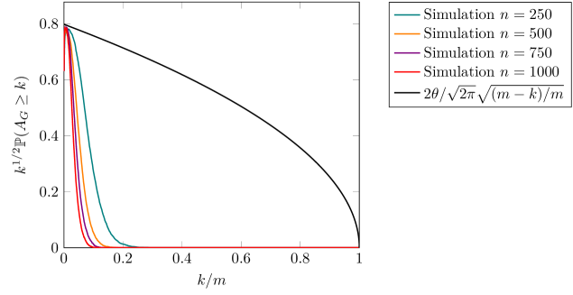
    Refer to caption
    Figure 5: Graph G=CS(n,4)G=CS(n,4).

    In contrast, we consider a graph G=CS(n,4)G=CS(n,4) consisting of nn star-components with 44 edges each, connected by a single path of edges connecting all the components. This graph thus consists of 5n5n vertices and also m=5nm=5n edges. We observe that as soon as one of the nn edges on the single path fails, the remaining graph is a (connected) tree. Therefore, with high probability, the graph would disconnect in two components both of order Θ(m)\Theta(m) after removing only a fixed number of edges. This effect is likely to occur again in both components when edges are removed uniformly at random in these components. This violates both properties we needed to prove our result for the configuration model. We observe in Figure 5 that indeed k1/2(ACSk)k^{1/2}\mathbb{P}\left(A_{CS}\geq k\right) does not seem to converge to a single function as nn\rightarrow\infty.

    References

    • [1] P. Bak and C. Tang. Earthquakes as a self-organized critical phenomenon. Journal of Geophysical Research: Solid Earth, 94(B11):15635–15637, 1989.
    • [2] P. Bak, C. Tang, and K. Wiesenfeld. Self-organized criticality: An explanation of the 1/f noise. Physical Review Letters, 59:381–384, 1987.
    • [3] P. Bak, C. Tang, and K. Wiesenfeld. Self-organized criticality. Physical Review A, 38:364–374, 1988.
    • [4] A. Barabási. The origin of bursts and heavy tails in human dynamics. Nature, 435(7039):207, 2005.
    • [5] A. Barabási and R. Albert. Emergence of scaling in random networks. Science, 286(5439):509–512, 1999.
    • [6] D. Bienstock. Electrical transmission system cascades and vulnerability - an operations research viewpoint, volume 22 of MOS-SIAM Series on Optimization. SIAM, 2016.
    • [7] B. A. Carreras, V. E. Lynch, I. Dobson, and D. E. Newman. Complex dynamics of blackouts in power transmission systems. Chaos: An Interdisciplinary Journal of Nonlinear Science, 14(3):643–652, 2004.
    • [8] B. K. Chakrabarti. A fiber bundle model of traffic jams. Physica A: Statistical Mechanics and its Applications, 372(1):162–166, 2006.
    • [9] A. Clauset, C. R. Shalizi, and M. E. J. Newman. Power-law distributions in empirical data. SIAM review, 51(4):661–703, 2009.
    • [10] D. Denisov, A. Sakhanenko, and V. Wachtel. First-passage times for random walks with nonidentically distributed increments. Ann. Probab., 46(6):3313–3350, 11 2018.
    • [11] S. Dhara, R. van der Hofstad, J. S. H. van Leeuwaarden, and S. Sen. Critical window for the configuration model: finite third moment degrees. Electronic Journal of Probability, 22:Paper No. 16, 33, (2017).
    • [12] R. A. Doney. Local behaviour of first passage probabilities. Probability Theory and Related Fields, 152(3):559–588, 2012.
    • [13] L. Federico and R. Hofstad. Critical window for connectivity in the configuration model. Combinatorics, Probability and Computing, 26(5):660–680, 2017.
    • [14] E. N. Gilbert. Random graphs. Annals of Mathematical Statistics, 30:1141–1144, (1959).
    • [15] P. E. Greenwood and A. A. Novikov. One-sided boundary crossing for processes with independent increments. Theory of Probability & Its Applications, 31(2):221–232, 1987.
    • [16] R. Hofstad. Random graphs and complex networks. Volume 1. Cambridge Series in Statistical and Probabilistic Mathematics. Cambridge University Press, Cambridge, (2017).
    • [17] S. Janson. The largest component in a subcritical random graph with a power law degree distribution. The Annals of Applied Probability, 18(4):1651–1668, (2008).
    • [18] S. Janson. On percolation in random graphs with given vertex degrees. Electronic Journal of Probability, 14:no. 5, 87–118, (2009).
    • [19] S. Janson. The probability that a random multigraph is simple. Combinatorics, Probability and Computing, 18(1-2):205–225, (2009).
    • [20] S. Janson. The probability that a random multigraph is simple. II. Journal of Applied Probability, 51A(Celebrating 50 Years of The Applied Probability Trust):123–137, (2014).
    • [21] H. Kesten. The critical probability of bond percolation on the square lattice equals 12{1\over 2}. Communications in Mathematical Physics, 74(1):41–59, (1980).
    • [22] H. Kesten and Y. Zhang. The probability of a large finite cluster in supercritical Bernoulli percolation. The Annals of Probability, 18(2):537–555, (1990).
    • [23] M. Korkali, J. G. Veneman, B. Tivnan, and P. Hines. Reducing cascading failure risk by increasing infrastructure network interdependency. Scientific Reports, 7, 10 2017.
    • [24] T. Łuczak. Sparse random graphs with a given degree sequence. In Random graphs, Vol. 2 (Poznań, 1989), Wiley-Intersci. Publ., pages 165–182. Wiley, New York, (1992).
    • [25] M. Molloy and B. Reed. A critical point for random graphs with a given degree sequence. In Proceedings of the Sixth International Seminar on Random Graphs and Probabilistic Methods in Combinatorics and Computer Science, “Random Graphs ’93” (Poznań, 1993), volume 6, pages 161–179, (1995).
    • [26] F. Morone and H. A. Makse. Influence maximization in complex networks through optimal percolation. Nature, 524(7563):65, 2015.
    • [27] A. E. Motter. Cascade control and defense in complex networks. Physical Review Letters, 93:098701, Aug 2004.
    • [28] A. E. Motter and Y. C. Lai. Cascade-based attacks on complex networks. Physical Review E, 66(065102), 2002.
    • [29] V. V. Petrov. Sums of Independent Random Variables. Ergebnisse der Mathematik und ihrer Grenzgebiete. Springer Berlin Heidelberg, 1975.
    • [30] S. Pradhan, A. Hansen, and B.K. Chakrabarti. Failure processes in elastic fiber bundles. Reviews of Modern Physics, 82(1):499–555, 2010.
    • [31] J. Qi, I. Dobson, and S. Mei. Towards estimating the statistics of simulated cascades of outages with branching processes. IEEE Transactions on Power Systems, 28(3):3410–3419, Aug 2013.
    • [32] H. A. Simon. On a clas of skew distribution functions. Biometrika, 42(3-4):425–440, 12 1955.
    • [33] F. Sloothaak, S. C. Borst, and B. Zwart. Robustness of power-law behavior in cascading line failure models. Stochastic Models, 34(1):45–72, 2018.
    • [34] F. Sloothaak, S. C. Borst, and B. Zwart. The impact of a network split on cascading failure processes. Stochastic Systems, 9(4):392–416, 2019.
    • [35] F. Sloothaak, V. Wachtel, and B. Zwart. First-passage time asymptotics over moving boundaries for random walk bridges. Journal of Applied Probability, 55(2):627–651, 2018.
    • [36] B. Suki, A. Barabási, Z. Hantos, F. Peták, and H. E. Stanley. Avalanches and power-law behaviour in lung inflation. Nature, 368(6472):615, 1994.
    • [37] K. Sun, Y. Hou, W. Sun, and J. Qi. Power System Control Under Cascading Failures: Understanding, Mitigation, and System Restoration. Wiley-IEEE Press, 2019.
    • [38] V. Wachtel and D. Denisov. An exact asymptotics for the moment of crossing a curved boundary by an asymptotically stable random walk. Theory of Probability & Its Applications, 60(3):481–500, 2016.
    • [39] Z. Wang, A. Scaglione, and R. J. Thomas. Generating statistically correct random topologies for testing smart grid communication and control networks. IEEE Transactions on Smart Grid, 1(1):28–39, June 2010.
    • [40] D.J. Watts. A simple model of global cascades on random networks. Proceedings of the National Academy of Sciences of the United States of America, 99(9):5766, 2002.
    • [41] J. Zheng, Z. Gao, X. Zhao, and F. Bai-Bai. Extended fiber bundle model for traffic jams on scale-free networks. International Journal of Modern Physics C (IJMPC), 19(11):1727–1735, 2008.

    Appendix A Lists of variables

    nn # vertices
    𝐝\mathbf{d} (Fixed) degree sequence
    m=mn(𝐝)m=m_{n}(\mathbf{d}) # edges in a configuration model with degree sequence 𝐝\mathbf{d}
    CMn(𝐝)CM_{n}(\mathbf{d}) Configuration model with degree sequence 𝐝\mathbf{d}
    CM¯n(𝐝)\overline{CM}_{n}(\mathbf{d}) Configuration model with degree sequence 𝐝\mathbf{d} conditioned to be connected
    nin_{i} # vertices with degree ii
    pip_{i} Fraction of vertices with degree ii
    DnD_{n} Degree of a vertex chosen uniformly at random from [n][n]
    DD Limiting degree variable of DnD_{n}
    dd Average degree of 𝐝\mathbf{d}
    θ\theta Disturbance constant
    ljm(i)l_{j}^{m}(i) Total load surge at edge jj after experiencing ii load surges in a graph with mm edges
    |Ejm(i)||E_{j}^{m}(i)| # edges in the component containing edge jj after experiencing ii load surges
    An,𝐝A_{n,\mathbf{d}} # edge failures after the cascading failure process
    Table 1: List of variables commonly used throughout this chapter.
    qq Removal probability in the percolation process
    CMn(𝐝,q)CM_{n}(\mathbf{d},q) Percolated configuration model with removal probability qq
    𝒞\mathcal{C} Component of a graph, sometimes also denoted as 𝒞(x)\mathcal{C}(x) when referring to the component that contains vertex or edge xx
    𝒞max\mathcal{C}_{\rm max} Largest component of a graph
    Tn,𝐝T_{n,\mathbf{d}} # edges that are sequentially removed uniformly at random for the first disconnection to occur in the connected configuration model
    TT Limiting variable of m1/2Tn,𝐝m^{1/2}T_{n,\mathbf{d}}
    |E^m(i)||\hat{E}_{m}(i)| # edges in the giant (largest) component after ii edges have been removed uniformly at random
    |E~m(i)||\tilde{E}_{m}(i)| # edges outside the giant (largest) component after ii edges have been removed uniformly at random
    Table 2: List of variables commonly used in percolation/sequential edge-removal process.
    RnR_{n} # removed half-edges in the first step of the explosion algorithm
    𝐝\mathbf{d}^{\prime} Degree sequence of configuration graph in step three of the explosion method (𝐝n+Rn\mathbf{d}^{\prime}\in\mathbb{N}^{n+R_{n}})
    CMN(𝐝)CM_{N}(\mathbf{d}^{\prime}) Configuration model in step three of the explosion method with degree sequence 𝐝\mathbf{d}^{\prime}
    CMn(𝐝,q)CM_{n}(\mathbf{d},q) Resulting configuration model in step four of the explosion method, indistinguishable from the percolated configuration model with removal probability qq
    nin_{i}^{\prime} # vertices of degree ii in CMN(𝐝)CM_{N}(\mathbf{d}^{\prime})
    pip_{i}^{\prime} limnni/n\lim_{n\rightarrow\infty}n_{i}^{\prime}/n
    nl,jn_{l,j} # vertices of degree ll in d that have degree jj in d\textbf{d}^{\prime}
    pl,jp_{l,j} Probability for a vertex of degree ll to retain jj half-edges after the first step of the explosion algorithm
    Lk(n)L_{k}^{\prime}(n) # components that are lines of length k2k\geq 2 in CMN(𝐝)CM_{N}(\mathbf{d}^{\prime})
    Ck(n)C_{k}^{\prime}(n) # components that are cycles of length k1k\geq 1 in CMN(𝐝)CM_{N}(\mathbf{d}^{\prime})
    Table 3: List of variables commonly used in the explosion algorithm.
    A^n,𝐝\hat{A}_{n,\mathbf{d}} # edges that were contained in the largest component upon failure during the cascade
    A~n,𝐝\tilde{A}_{n,\mathbf{d}} # edges that were contained outside the largest component upon failure during the cascade
    An+1A_{n+1}^{*} # edge failures in the cascading failure process on a star topology with n+1n+1 nodes and m=nm=n edges
    κ(i)\kappa(i) # edges that are contained in the largest component upon removal when ii edges are sequentially removed uniformly at random
    υ(i)\upsilon(i) Minimum # edges that need to be removed uniformly at random for the sum of υ(i)\upsilon(i) and # edges outside the giant to exceed ii
    ϱ(i)\varrho(i) # edges that need to be removed uniformly at random such that ii edges were contained in the giant component upon failure
    SiS_{i} j=1i(1Expj(1))\sum_{j=1}^{i}\left(1-\textrm{Exp}_{j}(1)\right)
    Li,mL_{i,m} Scaled perturbed load surge, formally defined as in (80)
    Si,mS_{i,m} Random walk defined as j=1iLj,mExpj,m(1)\sum_{j=1}^{i}L_{j,m}-\textrm{Exp}_{j,m}(1)
    Yi,mY_{i,m} Random walk j=1i(1Lj,m)\sum_{j=1}^{i}(1-L_{j,m})
    τm\tau_{m} First-passage time of random walk Si,mS_{i,m} to be less than 1θ1-\theta
    TgT_{g} First-passage time of random walk SiS_{i} to move below a boundary sequence (gi)i(g_{i})_{i\in\mathbb{N}}
    Table 4: List of variables commonly used in the failure process.

    Appendix B Proofs of results on the disintegration of the graph

    In this appendix, we present several proofs of results given in Section 3.

    Proof of Lemma 3.1.

    Due to the i.i.d. property of the surplus capacities, it holds that E~(i)\tilde{E}^{\prime}(i) has the distribution of ii edges chosen uniformly without repetitions from [m][m], so (E~(i)=B)=(mi)1\mathbb{P}(\tilde{E}^{\prime}(i)=B)=\binom{m}{i}^{-1}.

    Since all edges in CMn(𝐝,q)CM_{n}(\mathbf{d},q) are removed independently with probability qq, it holds for all sets BEB\subseteq E with |B|=i|B|=i that

    (E(G(q))=B)=qi(1q)mi,\displaystyle\mathbb{P}(E^{\prime}(G(q))=B)=q^{i}(1-q)^{m-i}, (86)

    while

    (|E(G(q))|=i)=(mi)qi(1q)mi.\displaystyle\mathbb{P}(|E^{\prime}(G(q))|=i)=\binom{m}{i}q^{i}(1-q)^{m-i}. (87)

    Since {E(G(q))=B}{|E(G(q))|=i}\{E^{\prime}(G(q))=B\}\subseteq\{|E^{\prime}(G(q))|=i\}, we obtain

    (E(G(q))=B|E(G(q))|=i)=(mi)1,\displaystyle\mathbb{P}(E^{\prime}(G(q))=B\mid|E^{\prime}(G(q))|=i)=\binom{m}{i}^{-1}, (88)

    so (12) holds. From (87) we obtain (13) by concentration of Bin(m,q)\textrm{Bin}(m,q) if qmqm\to\infty.

    Proof of Lemma 3.7.

    We use the explosion algorithm from Algorithm 1. To illustrate the type of arguments we use to prove this statement, we first consider the first moment only.

    Define 𝒱j\mathcal{V}_{j} as the set of all vertices of degree jj in 𝐝\mathbf{d}^{\prime}. Recall the degree sequence 𝐝\mathbf{d}^{\prime} from Lemma 3.4, and we define

    Lk={{v1,v2,,vk}:v1,vk𝒱1;v2,,vk1𝒱2},\displaystyle L_{k}=\{\{v_{1},v_{2},...,v_{k}\}:v_{1},v_{k}\in\mathcal{V}_{1};v_{2},...,v_{k-1}\in\mathcal{V}_{2}\},

    the set of all collections of kk vertices that could form a line. Note that

    Lk(n)=lk𝟙{l forms a line}.\displaystyle L_{k}^{\prime}(n)=\sum_{l\in\mathcal{L}_{k}}\mathbbm{1}_{\{l\text{ forms a line}\}}.

    Due to Lemma 3.4, we observe that

    𝔼\displaystyle\mathbb{E} [Lk(n)]=𝔼[lk𝟙{l forms a line}]\displaystyle[L_{k}^{\prime}(n)]=\mathbb{E}\left[\sum_{l\in\mathcal{L}_{k}}\mathbbm{1}_{\{l\text{ forms a line}\}}\right]
    =𝔼[(n12)(n2k2)2k42m12k62m322m2k+512m2k+3]\displaystyle=\mathbb{E}\left[\binom{n_{1}^{\prime}}{2}\binom{n_{2}^{\prime}}{k-2}\frac{2k-4}{2m-1}\frac{2k-6}{2m-3}\cdots\frac{2}{2m-2k+5}\frac{1}{2m-2k+3}\right]
    =𝔼[n12n2k22(k2)!(2k4)!!(2m)k1](1+o(1))=i2m14(1+2p2d)2(2p2d)k2(1+o(1)).\displaystyle=\mathbb{E}\left[\frac{{n_{1}^{\prime}}^{2}{n_{2}^{\prime}}^{k-2}}{2(k-2)!}\frac{(2k-4)!!}{(2m)^{k-1}}\right](1+o(1))=\frac{i^{2}}{m}\frac{1}{4}\Big{(}1+\frac{2p_{2}}{d}\Big{)}^{2}\Big{(}\frac{2p_{2}}{d}\Big{)}^{k-2}(1+o(1)).

    Next, we generalize these arguments to higher and mixed moments of the variables (Lk(n))n2(L_{k}^{\prime}(n))_{n\geq 2}. We follow the same approach used in [13] where the convergence of the number of lines to a sequence of Poisson variables was proved in the critical window for connectivity. Using the method of moments, in this case, we need to prove concentration of the number of vertices and edges in line components.

    We prove (39) by induction. With a slight abuse of notation, we start the induction step at k=1k=1, or alternatively, at k=2k=2 with r2=0r_{2}=0. Then, both sides in (39) are equal to one, and hence the induction hypothesis is satisfied.

    Next, we show how to advance the induction hypothesis. We define

    Wk(𝐫)={j=2k{lj(1),,lj(rj)}:lj(h)j for all 1hrj,2jk},\displaystyle W_{k}(\mathbf{r})=\left\{\bigcup_{j=2}^{k}\{l_{j}(1),...,l_{j}(r_{j})\}:l_{j}(h)\in\mathcal{L}_{j}\textrm{ for all }1\leq h\leq r_{j},2\leq j\leq k\right\},

    the collection of sets of j=2krj\sum_{j=2}^{k}r_{j} possible lines. Moreover, for a set wk(𝐫)Wk(𝐫)w_{k}(\mathbf{r})\in W_{k}(\mathbf{r}), we define (wk(𝐫))\mathcal{E}(w_{k}(\mathbf{r})) as the event that all elements in the set wk(𝐫)w_{k}(\mathbf{r}) form a line component in CMN(𝐝)CM_{N}(\mathbf{d}^{\prime}). Then, using the tower property, we can rewrite

    𝔼[L2(n)r2Lk(n)rh]=𝔼[wk(𝐫)Wk(𝐫)𝟙(wk(𝐫))]\displaystyle\mathbb{E}[L_{2}^{\prime}(n)^{r_{2}}\cdots L_{k}^{\prime}(n)^{r_{h}}]=\mathbb{E}\left[\sum_{w_{k}(\mathbf{r})\in W_{k}(\mathbf{r})}\mathbbm{1}_{\mathcal{E}(w_{k}(\mathbf{r}))}\right]
    =𝔼[wk1(𝐫)𝟙(wk1(𝐫))𝔼[lk(1),,lk(rk)k𝟙lk(1)𝟙lk(2)𝟙lk(rk)(wk1(𝐫))]],\displaystyle=\mathbb{E}\left[\sum_{w_{k-1}(\mathbf{r})}\mathbbm{1}_{\mathcal{E}(w_{k-1}(\mathbf{r}))}\mathbb{E}\left[\sum_{l_{k}(1),\ldots,l_{k}(r_{k})\in\mathcal{L}_{k}}\mathbbm{1}_{l_{k}(1)}\mathbbm{1}_{l_{k}(2)}\cdots\mathbbm{1}_{l_{k}(r_{k})}\mid\mathcal{E}(w_{k-1}(\mathbf{r}))\right]\right],

    where 𝟙lk(h)\mathbbm{1}_{l_{k}(h)} denotes the indicator of the event that the set lk(h)l_{k}(h) forms a line. Next, we show that for every wk(𝐫)Wk(𝐫)w_{k}(\mathbf{r})\in W_{k}(\mathbf{r}),

    (mi2)rklk(1),,lk(rk)k\displaystyle\Big{(}\frac{m}{i^{2}}\Big{)}^{r_{k}}\sum_{l_{k}(1),\ldots,l_{k}(r_{k})\in\mathcal{L}_{k}} 𝔼[𝟙lk(1)𝟙lk(2)𝟙lk(rk)|(wk1(𝐫))]\displaystyle\mathbb{E}[\mathbbm{1}_{l_{k}(1)}\mathbbm{1}_{l_{k}(2)}\cdots\mathbbm{1}_{l_{k}(r_{k})}|\mathcal{E}(w_{k-1}(\mathbf{r}))]
    =(14(1+2p2d)2(2p2d)k2)rk(1+o(1)).\displaystyle=\left(\frac{1}{4}\Big{(}1+\frac{2p_{2}}{d}\Big{)}^{2}\Big{(}\frac{2p_{2}}{d}\Big{)}^{k-2}\right)^{r_{k}}(1+o(1)).

    Note that by induction, this suffices to conclude (39).

    First, note that if any of the lk(j),1jrk,l_{k}(j),1\leq j\leq r_{k}, contains any of the vertices used in wk1(𝐫)w_{k-1}(\mathbf{r}), then it is not possible for it to form a line of length kk as these vertices are already contained in line components of a smaller length. In that case, 𝔼[𝟙lk(1)𝟙lk(2)𝟙lk(rk)(wk1(𝐫))]=0\mathbb{E}[\mathbbm{1}_{l_{k}(1)}\mathbbm{1}_{l_{k}(2)}\cdots\mathbbm{1}_{l_{k}(r_{k})}\mid\mathcal{E}(w_{k-1}(\mathbf{r}))]=0. Therefore, we can consider the part of the graph excluding the line components in wk1(𝐫)w_{k-1}(\mathbf{r}). This part of the graph is also a configuration model, but with a slightly altered degree sequence. Note that we exclude finitely many line components of finite length, and hence only exclude finitely many vertices and edges. With a slight abuse of notation, write r=r(lk(1),,lk(rk))r^{\prime}=r^{\prime}(l_{k}(1),...,l_{k}(r_{k})) as the number of mutually distinct lines. Then the probability that rr^{\prime} mutually distinct lines can be formed in the graph excluding the line components in wk1(𝐫)w_{k-1}(\mathbf{r}) is given by

    𝔼[𝟙lk(1)𝟙lk(2)𝟙lk(rk)|(wk1(𝐫))]=(2k4)!!r(2m)r(k1)(1+o(1)).\displaystyle\mathbb{E}[\mathbbm{1}_{l_{k}(1)}\mathbbm{1}_{l_{k}(2)}\cdots\mathbbm{1}_{l_{k}(r_{k})}|\mathcal{E}(w_{k-1}(\mathbf{r}))]=\frac{(2k-4)!!^{r^{\prime}}}{(2m)^{r^{\prime}(k-1)}}(1+o(1)).

    We sum these contributions over the number of possible sets that exist in the subgraph. Write C(rk,r)C(r_{k},r^{\prime}) as the number of distinct sets of rkr_{k} lines that contain the same set of rr^{\prime} mutually distinct lines of length kk. Importantly, C(rk,rk)=1C(r_{k},r_{k})=1 and C(rk,r)C(r_{k},r^{\prime}) is a finite integer if 1rrk11\leq r^{\prime}\leq r_{k}-1. Recalling Lemma 3.4, we obtain

    (mi2)rk\displaystyle\Big{(}\frac{m}{i^{2}}\Big{)}^{r_{k}} lk(1),,lk(rk)k𝔼[𝟙lk(1)𝟙lk(2)𝟙lk(rk)|(wk1(𝐫))]\displaystyle\sum_{l_{k}(1),\ldots,l_{k}(r_{k})\in\mathcal{L}_{k}}\mathbb{E}[\mathbbm{1}_{l_{k}(1)}\mathbbm{1}_{l_{k}(2)}\cdots\mathbbm{1}_{l_{k}(r_{k})}|\mathcal{E}(w_{k-1}(\mathbf{r}))]
    =(mi2)rk𝔼[r=1rkC(rk,r)(n12n2k22(k2)!(2k4)!!(2m)k1)r](1+o(1))\displaystyle=\Big{(}\frac{m}{i^{2}}\Big{)}^{r_{k}}\mathbb{E}\left[\sum_{r^{\prime}=1}^{r_{k}}C(r_{k},r^{\prime})\left(\frac{{n_{1}^{\prime}}^{2}{n_{2}^{\prime}}^{k-2}}{2(k-2)!}\frac{(2k-4)!!}{(2m)^{k-1}}\right)^{r^{\prime}}\right](1+o(1))
    =(14(1+2p2d)2(2p2d)k2)rk(1+o(1)),\displaystyle=\left(\frac{1}{4}\Big{(}1+\frac{2p_{2}}{d}\Big{)}^{2}\Big{(}\frac{2p_{2}}{d}\Big{)}^{k-2}\right)^{r_{k}}(1+o(1)),

    concluding the proof.

    Proof of Corolllary 3.8.

    Note that it follows from Lemma 3.7

    𝔼[Lk(n)]\displaystyle\mathbb{E}[L_{k}^{\prime}(n)] =i2m14(1+2p2d)2(2p2d)k2(1+o(1)),k2.\displaystyle=\frac{i^{2}}{m}\frac{1}{4}\Big{(}1+\frac{2p_{2}}{d}\Big{)}^{2}\Big{(}\frac{2p_{2}}{d}\Big{)}^{k-2}(1+o(1)),\hskip 28.45274ptk\geq 2.

    Consequently, for every ε>0\varepsilon>0 there exists a N>0N>0 such that for all nNn\geq N,

    mi2𝔼[Lk(n)]14(1+2p2+εdε)2(2p2+εdε)k2,k2.\displaystyle\frac{m}{i^{2}}\mathbb{E}[L_{k}^{\prime}(n)]\leq\frac{1}{4}\Big{(}1+\frac{2p_{2}+\varepsilon}{d-\varepsilon}\Big{)}^{2}\Big{(}\frac{2p_{2}+\varepsilon}{d-\varepsilon}\Big{)}^{k-2},\hskip 28.45274ptk\geq 2.

    In particular, for ε\varepsilon small enough 2p2+εdε<1\frac{2p_{2}+\varepsilon}{d-\varepsilon}<1 so that the sequence converges to zero exponentially fast in kk. We apply dominated convergence to obtain

    𝔼[mi2k=2kLk(n)]\displaystyle\mathbb{E}\Big{[}\frac{m}{i^{2}}\sum_{k=2}^{\infty}kL_{k}^{\prime}(n)\Big{]} (dp2)(d+2p2)22d(d2p2)2,\displaystyle\to\frac{(d-p_{2})(d+2p_{2})^{2}}{2d(d-2p_{2})^{2}}, (89)
    𝔼[mi2k=2(k1)Lk(n)]\displaystyle\mathbb{E}\Big{[}\frac{m}{i^{2}}\sum_{k=2}^{\infty}(k-1)L_{k}^{\prime}(n)\Big{]} (d+2p2)24(d2p2)2.\displaystyle\to\frac{(d+2p_{2})^{2}}{4(d-2p_{2})^{2}}. (90)

    In other words, we have derived the expected number of vertices and edges in line components in CMN(𝐝)CM_{N}(\mathbf{d}^{\prime}). Next, we prove (40) for every j2j\geq 2. We define for a sequence 𝐫\mathbf{r} of positive integer values, |𝐫|1=h=1krh|\mathbf{r}|_{1}=\sum_{h=1}^{k}r_{h}, i.e. its 1\ell_{1} norm. We write

    𝔼[(mi2k=2kLk(n))j]=mji2j𝐫:|𝐫|1=jh2𝔼[(hLh(n))rh].\displaystyle\mathbb{E}\Big{[}\Big{(}\frac{m}{i^{2}}\sum_{k=2}^{\infty}kL_{k}^{\prime}(n)\Big{)}^{j}\Big{]}=\frac{m^{j}}{i^{2j}}\sum_{\mathbf{r}:|\mathbf{r}|_{1}=j}\prod_{h\geq 2}\mathbb{E}[(hL_{h}^{\prime}(n))^{r_{h}}].

    For every ε0\varepsilon\geq 0, it holds for all nn sufficiently large that

    (mi2)|𝐫|1h2𝔼[(Lh(n))rh]14|𝐫|1(1+2p2+εdε)2|𝐫|1(2p2+εdε)h2(h2)rh.\displaystyle\Big{(}\frac{m}{i^{2}}\Big{)}^{|\mathbf{r}|_{1}}\prod_{h\geq 2}\mathbb{E}[(L_{h}^{\prime}(n))^{r_{h}}]\leq\frac{1}{4^{|\mathbf{r}|_{1}}}\Big{(}1+\frac{2p_{2}+\varepsilon}{d-\varepsilon}\Big{)}^{2|\mathbf{r}|_{1}}\Big{(}\frac{2p_{2}+\varepsilon}{d-\varepsilon}\Big{)}^{\sum_{h\geq 2}(h-2)r_{h}}. (91)

    If ε\varepsilon is small enough, then 2p2+εdε<1\frac{2p_{2}+\varepsilon}{d-\varepsilon}<1, and thus the sequence is decreasing exponentially fast in h2hrh\sum_{h\geq 2}hr_{h}. Applying dominated convergence thus yields (40).

    Appendix C Proofs of results on the cascading failure process

    Proof of Lemma 4.6.

    First, we observe that

    (Tg>k)(T1θ>k),\displaystyle\mathbb{P}\left(T_{g^{-}}>k\right)\geq\mathbb{P}\left(T_{1-\theta}>k\right),

    and hence it suffices to show that the reversed inequality holds asymptotically. Our proof will be similar to the proof of Lemma 4.4, but adapted to provide an upper bound.

    Fix ϵ>0\epsilon>0 small as in Lemma 4.4, and define the piecewise constant boundary

    h^i,kϵ={h(0)=1θif it0,kϵ=l,h(j)if tj1,kϵ<itj,kϵ, 1jr1,h(r)if i>tr1,kϵ.\displaystyle\hat{h}_{i,k}^{\epsilon}=\left\{\begin{array}[]{ll}h^{(0)}=1-\theta&\textrm{if }i\leq t_{0,k}^{\epsilon}=l,\\ -h^{(j)}&\textrm{if }t_{j-1,k}^{\epsilon}<i\leq t_{j,k}^{\epsilon},\;1\leq j\leq r-1,\\ -h^{(r)}&\textrm{if }i>t_{r-1,k}^{\epsilon}.\end{array}\right.

    for rr, times tj,kϵt_{j,k}^{\epsilon} and levels h(j)h^{(j)} defined as in the proof of Lemma 4.4. We note that for every fixed δ>0\delta>0,

    (Tg>k)(Th^ϵ>k;Stj,kϵ(δtj,kϵ,1/δtj,kϵ), 0jr1)\displaystyle\mathbb{P}\left(T_{g^{-}}>k\right)\leq\mathbb{P}\left(T_{\hat{h}^{\epsilon}}>k;S_{t_{j,k}^{\epsilon}}\in\left(\delta\sqrt{t_{j,k}^{\epsilon}},1/\delta\sqrt{t_{j,k}^{\epsilon}}\right),\;\;\;\forall\,0\leq j\leq r-1\right)
    +j=0r(Tg>k;Stj,kϵ(δtj,kϵ,1/δtj,kϵ)).\displaystyle\hskip 142.26378pt+\sum_{j=0}^{r}\mathbb{P}\left(T_{g^{-}}>k;S_{t_{j,k}^{\epsilon}}\not\in\left(\delta\sqrt{t_{j,k}^{\epsilon}},1/\delta\sqrt{t_{j,k}^{\epsilon}}\right)\right).

    Using analogous arguments as in Lemma 4.4, we obtain

    (Th^ϵ>k;Stj,kϵ(δtj,kϵ,1/δtj,kϵ), 0jr1)\displaystyle\mathbb{P}\left(T_{\hat{h}^{\epsilon}}>k;S_{t_{j,k}^{\epsilon}}\in\left(\delta\sqrt{t_{j,k}^{\epsilon}},1/\delta\sqrt{t_{j,k}^{\epsilon}}\right),\;\;\;\forall\,0\leq j\leq r-1\right)
    (1+o(1))(T1θ>k).\displaystyle\hskip 227.62204pt\leq(1+o(1))\mathbb{P}\left(T_{1-\theta}>k\right).

    For the other terms, define the sequence (h~i)i(\tilde{h}_{i})_{i\in\mathbb{N}} with h~i=min{1θ,iγ}\tilde{h}_{i}=\min\{1-\theta,-i^{\gamma}\}. Then, due to Theorem 1 of [10],

    j=0r\displaystyle\sum_{j=0}^{r} (Tg>k;Stj,kϵ(δtj,kϵ,1/δtj,kϵ))\displaystyle\mathbb{P}\left(T_{g^{-}}>k;S_{t_{j,k}^{\epsilon}}\not\in\left(\delta\sqrt{t_{j,k}^{\epsilon}},1/\delta\sqrt{t_{j,k}^{\epsilon}}\right)\right)
    j=0r1(Stj,kϵ(δtj,kϵ,1/δtj,kϵ)|Th~>k)(Th~>k)\displaystyle\hskip 56.9055pt\leq\sum_{j=0}^{r-1}\mathbb{P}\left(S_{t_{j,k}^{\epsilon}}\not\in\left(\delta\sqrt{t_{j,k}^{\epsilon}},1/\delta\sqrt{t_{j,k}^{\epsilon}}\right)\big{|}T_{\tilde{h}}>k\right)\mathbb{P}\left(T_{\tilde{h}}>k\right)
    (1+o(1))r(1eδ22+e12δ2)(Th~>k).\displaystyle\hskip 56.9055pt\leq(1+o(1))r\left(1-e^{-\frac{\delta^{2}}{2}}+e^{-\frac{1}{2\delta^{2}}}\right)\mathbb{P}\left(T_{\tilde{h}}>k\right).

    Letting δ0\delta\downarrow 0 yields [10]

    j=0r\displaystyle\sum_{j=0}^{r} (Tg>k;Stj,kϵ(δtj,kϵ,1/δtj,kϵ))=o((Th~>k))=o(k1/2).\displaystyle\mathbb{P}\left(T_{g^{-}}>k;S_{t_{j,k}^{\epsilon}}\not\in\left(\delta\sqrt{t_{j,k}^{\epsilon}},1/\delta\sqrt{t_{j,k}^{\epsilon}}\right)\right)=o\left(\mathbb{P}\left(T_{\tilde{h}}>k\right)\right)=o\left(k^{-1/2}\right).

    Since

    (T1θ>k)2θ2πk1/2,\displaystyle\mathbb{P}\left(T_{1-\theta}>k\right)\sim\frac{2\theta}{\sqrt{2\pi}}k^{-1/2},

    we conclude that

    lim supk(Tg>k)(T1θ>k)1.\displaystyle\limsup_{k\rightarrow\infty}\frac{\mathbb{P}\left(T_{g^{-}}>k\right)}{\mathbb{P}\left(T_{1-\theta}>k\right)}\leq 1.

    Proof of Lemma 4.10.

    This statement is a consequence of Theorem 2.3. Recall that by definition,

    υ(k)+|E~m(υ(k))|k,\displaystyle\upsilon(k)+|\tilde{E}_{m}(\upsilon(k))|\geq k,

    and υ(k)k\upsilon(k)\leq k. Moreover,

    |E~m(υ(k))|=mυ(k)|E^m(υ(k))|max1jk{mj|E^m(j)|}.\displaystyle|\tilde{E}_{m}(\upsilon(k))|=m-\upsilon(k)-|\hat{E}_{m}(\upsilon(k))|\leq\max_{1\leq j\leq k}\left\{m-j-|\hat{E}_{m}(j)|\right\}.

    It follows that

    (|E~m(υ(k))|kα)\displaystyle\mathbb{P}\left(|\tilde{E}_{m}(\upsilon(k))|\geq k^{\alpha}\right) (max1jk{mj|E^m(j)|}kα)\displaystyle\leq\mathbb{P}\left(\max_{1\leq j\leq k}\left\{m-j-|\hat{E}_{m}(j)|\right\}\geq k^{\alpha}\right)
    (max1jk{mj|E^m(j)|}jα)=o(m1/2)\displaystyle\leq\mathbb{P}\left(\max_{1\leq j\leq k}\left\{m-j-|\hat{E}_{m}(j)|\right\}\geq j^{\alpha}\right)=o(m^{-1/2})

    by Theorem 2.3. We conclude that

    (υ(k)kkα)(|E~m(υ(k))|kα)=o(m1/2).\displaystyle\mathbb{P}\left(\upsilon(k)\leq k-k^{\alpha}\right)\leq\mathbb{P}\left(|\tilde{E}_{m}(\upsilon(k))|\geq k^{\alpha}\right)=o(m^{-1/2}).

    Proof of Lemma 4.11.

    Again, this is a consequence of Theorem 2.3. We note that for every 1lm1\leq l\leq m,

    κ(l)=i=1sBer(πi+1),\displaystyle\kappa(l)=\sum_{i=1}^{s}\textrm{Ber}(\pi_{i+1}),

    where

    πi=|E^m(i2)|mi+2\displaystyle\pi_{i}=\frac{|\hat{E}_{m}(i-2)|}{m-i+2}

    is a random variable. Due to Theorem 2.3,

    (πi1iαmi+2 for some 2ik+1)=o(m1/2).\displaystyle\mathbb{P}\left(\pi_{i}\leq 1-\frac{i^{\alpha}}{m-i+2}\textrm{ for some }2\leq i\leq k+1\right)=o(m^{-1/2}).

    Since for every α(0,1)\alpha\in(0,1), the function iα1/(mi+1)i^{\alpha-1}/(m-i+1) is an increasing function in ii, it follows that

    (πi1kα1 for some 2ik+1)=o(m1/2).\displaystyle\mathbb{P}\left(\pi_{i}\leq 1-k^{\alpha-1}\textrm{ for some }2\leq i\leq k+1\right)=o(m^{-1/2}).

    We derive the bound

    (ϱ(k)>k+kα)\displaystyle\mathbb{P}\left(\varrho(k)>k+k^{\alpha}\right) =(κ(k+k(α+1)/2)k)(i=1k+k(α+1)/2Ber(πi+1)k)\displaystyle=\mathbb{P}\left(\kappa\left(k+k^{(\alpha+1)/2}\right)\leq k\right)\leq\mathbb{P}\left(\sum_{i=1}^{k+k^{(\alpha+1)/2}}\textrm{Ber}(\pi_{i+1})\leq k\right)
    (i=1k+k(α+1)/2Ber(kα1)>k(α+1)/2)\displaystyle\leq\mathbb{P}\left(\sum_{i=1}^{k+k^{(\alpha+1)/2}}\textrm{Ber}(k^{\alpha-1})>k^{(\alpha+1)/2}\right)
    exp{12k(1α)/2(1+o(1))}=o(m1/2),\displaystyle\leq\exp\left\{-\frac{1}{2}k^{(1-\alpha)/2}(1+o(1))\right\}=o(m^{-1/2}),

    where the last inequality is due to the Chernoff bound.