Faddeev calculations of low-energy $\Lambda$ -deuteron scattering
and momentum correlation function

M. Kohno Research Center for Nuclear Physics, Osaka University, Ibaraki 567-0047, Japan H. Kamada Department of Physics, Faculty of Engineering, Kyushu Institute of Technology, Kitakyushu 804-8550, Japan Research Center for Nuclear Physics, Osaka University, Ibaraki 567-0047, Japan

Abstract

Faddeev calculations of low-energy $\Lambda$ -deuteron elastic scattering are performed up to $E_{cm}=20$ MeV crossing the deuteron threshold. The phase shifts of the $s$ wave with $J=1/2$ and $J=3/2$ are calculated using strangeness $S=-1$ hyperon-nucleon interactions in chiral effective field theory NLO13 and NLO19 parametrized by the Jülich-Bonn group. The effective range parameters, specifically the scattering length and effective range, are ascertained through the calculated phase shifts. The present study evaluates the momentum correlation functions of the $\Lambda$ -deuteron system using the $\Lambda$ -deuteron relative wave function, constructed from half-off-shell $t$ matrices. The results are then compared with those obtained using an approximate formula.

I Introduction

An accurate description of $\Lambda$ -nucleon interactions is essential for achieving a microscopic understanding of $\Lambda$ hypernuclei. This understanding is being sought through the collection of increasingly accurate experimental data at several facilities TAM22 . Furthermore, this knowledge is also crucial to understanding the role of $\Lambda$ hyperons in neutron-star matter. Although various theoretical descriptions of the $\Lambda$ -nucleon interaction have been developed over the past several decades, the quality of these models remains comparatively inferior to that of $NN$ potentials, largely due to the scarceness of available scattering data. The absence of the $\Lambda N$ two-body bound state is a significant disadvantage. Then, the lightest hypernucleus, ${}_{\Lambda}^{3}$ H, plays a crucial role in investigating the $\Lambda$ N interactions to determine the $s$ -wave strength, despite the difficulty in controlling the relative ratio of singlet and triplet channels. However, the shallow separation energy of ${}_{\Lambda}^{3}$ H to $\Lambda$ and deuteron has not been adequately determined and has a considerable error bar. The current world average is $164\pm 43$ keV MA2023 . There is a problem with the presence of $\Lambda NN$ three-body forces (3BFs) on the theoretical side. It is crucial to understand the role of the 3BFs quantitatively. We have carried out Faddeev calculations for ${}_{\Lambda}^{3}$ H KKM22 using next-to-leading order (NLO) hyperon-nucleon ( $YN$ ) interactions and $YNN$ 3BFs provided by the expressions in the next-to-next-to leading order (NNLO) in chiral effective field theory (ChEFT). The net contribution of the 3BFs is not negligible but is of a similar magnitude as the present experimental uncertainty. However, the result depends on the low-energy constants which are difficult to fix without investigations of heavier hypernuclei. After observing the order of magnitude of the 3BF effect in the bound ${}_{\Lambda}^{3}$ H, it is worthwhile to study the role of $\Lambda$ N interactions in scattering processes.

There are several theoretical studies in the literature on the properties of the $\Lambda d$ scattering. Garcilazo et al. GAR75 ; GAR76 used bound state Faddeev calculations to estimate effective range parameters. Hammer et al. HWH02 ; HH19 carried out studies within the framework of pionless effective field theory. Schäfer et al. SCH22 discussed the $J=3/2$ $\Lambda d$ phase shift in low energies based on varying effective range parameters. However, no explicit calculation of the $\Lambda d$ elastic scattering has been performed by solving Faddeev equations using modern $YN$ interactions.

In this article, we consider $\Lambda$ -deuteron scattering problems in a Faddeev formulation using chiral $NN$ and $YN$ interactions, although 3BFs are not incorporated. While the data from direct low-energy $\Lambda d$ scattering experiments are still forthcoming, the $\Lambda$ d correlation functions observed in heavy-ion collision experiments FAB21 have already provided valuable insights into the interactions between $\Lambda$ and the deuteron as well as between $\Lambda$ and the proton. The preliminary results of the $\Lambda d$ correlation functions were reported in a report HU24 based on 3 GeV Au+Au collisions by the STAR collaboration. The correlation function depends on the $\Lambda d$ relative wave function, which is controlled by the interaction between $\Lambda$ and deuteron arising from $\Lambda N$ interactions controls. Thus far, theoretical investigations of the $\Lambda d$ correlation function have been carried out HAID20 using an asymptotic wave function approximated by effective range parameters of the scattering amplitude LL82 . It is worthwhile to calculate the corresponding correlation function using the $\Lambda d$ wave function obtained by solving the Faddeev equation for the $\Lambda$ scattering process on the deuteron.

The deuteron is a two-body composite system, and thus the momentum correlation function is affected by the dynamics associated with its formation. The problem was studied by Mrówozyński MR20 and actual calculations for the nucleon-deuteron correlation functions were performed by Viviani et al. VIV23 . Similar calculations for the $\Lambda d$ case are possible in the present Faddeev treatment of the $\Lambda d$ scattering, which is a subject of future investigation.

The Faddeev equations for the $\Lambda$ -deuteron ( $\Lambda d$ ) scattering are outlined in Sec. II, based on the formulation by Glöckle et al. GL96 . The equations in a partial wave representation and the treatment of two types of singularities, a moving singularity and a deuteron pole, are outlined in Appendices A $-$ C. The numerical results for the $s$ -wave phase shift up to $E_{cm}=20$ MeV are presented in Sec. III. The parameters of the effective range expansion, i.e., the scattering length and effective range, are estimated based on the obtained phase shifts. The radial $\Lambda d$ wave function is evaluated and $\Lambda d$ correlation functions corresponding to the measured ones in heavy-ion experiments are calculated. A summary is provided in Sec. IV.

II Faddeev equations for $\Lambda$ -deuteron scattering

We follow the derivation of the equations describing three-body scattering problems in Ref. GL96 . Two nucleons are denoted by labels 1 and 2. The $\Lambda$ hyperon is assigned label 3. The mass difference of the proton and neutron is discarded. In the present treatment, three-body $\Sigma NN$ states are not incorporated explicitly, although the $\Lambda N$ - $\Sigma N$ coupling is included in solving $\Lambda N$ $t$ matrices. Three-body interactions are not considered.

The process of the $\Lambda$ -hyperon scattering on the bound deuteron is described by the following set of equations:

$\displaystyle u_{3}\phi=$	$\displaystyle t_{1}G_{0}u_{1}\phi+t_{2}G_{0}u_{2}\phi,$	(1)
$\displaystyle u_{1}\phi=$	$\displaystyle G_{0}^{-1}\phi+t_{3}G_{0}u_{3}\phi+t_{2}G_{0}u_{2}\phi,$	(2)
$\displaystyle u_{2}\phi=$	$\displaystyle G_{0}^{-1}\phi+t_{3}G_{0}u_{3}\phi+t_{1}G_{0}u_{1}\phi,$	(3)

which correspond to Eqs. (36) $-$ (41) of Ref. GL96 with the replacement as $\phi_{1}\rightarrow\phi$ , $U_{11}\rightarrow u_{3}$ , $U_{21}\rightarrow u_{1}$ , and $U_{31}\rightarrow u_{2}$ . $G_{0}$ is a three-body Green function and $t_{i}$ is a pertinent two-body $t$ matrix. Because the two-nucleon state is antisymmetric, Eqs. (2) and (3) are equivalent, and the above equations reduce to

	$\displaystyle u_{3}\phi=$	$\displaystyle(1-P_{12})t_{2}G_{0}u_{2}\phi,$		(4)
	$\displaystyle u_{2}\phi=$	$\displaystyle G_{0}^{-1}\phi+t_{3}G_{0}u_{3}\phi-P_{12}t_{2}G_{0}u_{2}\phi,$		(5)

where $P_{12}$ denotes the exchange operation for nucleons 1 and 2. In actual calculations, it is convenient to introduce $T_{i}\equiv t_{i}G_{0}u_{i}$ . The above equations are rewritten as follows:

	$\displaystyle T_{3}\phi=$	$\displaystyle t_{3}G_{0}(1-P_{12})T_{2}\phi,$		(6)
	$\displaystyle T_{2}\phi=$	$\displaystyle t_{2}\phi+t_{2}G_{0}T_{3}\phi-t_{2}P_{12}G_{0}T_{2}\phi.$		(7)

Refer to caption — Figure 1: Jacobi coordinates.

These equations are solved in a partial wave representation in momentum space. Two sets of the Jacobi momenta $(\mbox{\boldmath$p$}_{j},\mbox{\boldmath$q$}_{j})$ with $j=2,\;3$ are defined as in Fig. 1. The partial wave three-body state in a Jacobi momentum space is denoted as

	$\displaystyle\|p_{j}q_{j}\alpha_{j}\rangle=$	$\displaystyle\|p_{j}q_{j};[[\ell_{p_{j}}\times s_{p_{j}}]^{j}\times[\lambda_{q_{j}}\times s_{q_{j}}]^{I}]^{J}_{M},$
		$\displaystyle[t_{p_{j}}\times t_{q_{j}}]^{T}_{M_{T}}\rangle,$		(8)

where an abbreviated notation for an angular-momentum coupling with Clebsch-Gordan coefficients is used:

[\ell\times s]^{j}_{m_{j}}=\sum_{m_{\ell}m_{s}}(\ell m_{\ell}sm_{s}|j_{m_{j}})Y_{\ell m_{\ell}}(\hat{\mbox{\boldmath$p$}})\chi_{sm_{s}}.

(9)

Here, $Y_{\ell m_{\ell}}$ is a spherical harmonic function, and $\chi_{sm_{s}}$ represents a spin state.

By solving the simultaneous equations (6) and (7), the $T$ matrix of the elastic $\Lambda$ -deuteron scattering is obtained GL96 by

T=\langle\phi|(1-P_{12})T_{2}|\phi\rangle=2\langle\phi|T_{2}|\phi\rangle

(10)

The $S$ -matrix is related to the $T$ -matrix as

S=1-2\pi i\mu_{\Lambda d}kT,

(11)

where $\mu_{\Lambda d}$ is a reduced mass of the $\Lambda$ and deuteron, and $k$ is the $\Lambda$ -deuteron relative momentum.

Explicit equations in a partial wave representation are presented in Appendix A. In solving these equations numerically, there are difficulties in treating two types of singularities. One appears in the Green function $G_{0}$ , which is known as a moving singularity. This singularity is treated by a standard subtraction method in evaluating the matrix elements. The other one is the deuteron pole, which has to be taken care of when $T_{3}$ is substituted in Eq. (7). The way to treat the deuteron pole and the moving singularity is outlined in Appendicies A and B.

III Calculated results

In this section, we present the results of the Faddeev calculations for low-energy $\Lambda$ -deuteron elastic scattering in an $s$ wave up to $E_{cm}=20$ MeV using two versions of chiral NLO $S=-1$ $YN$ interactions, NLO13 NLO13 and NLO19 NLO19 . As for the $NN$ interaction, the chiral N⁴LO⁺ interaction RKE18 is used. The cutoff scale is 550 MeV for both $NN$ and $YN$ interactions.

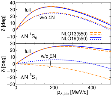
Before presenting the results of the $\Lambda d$ scattering, it is instructive to show ¹S₀ and ³S₁ phase shifts of the $\Lambda N$ scattering with NLO13 and NLO19. Figure 2 shows those results. Phase shifts obtained by switching off the $\Lambda N$ - $\Sigma N$ coupling are included to show the difference between the characters of two interactions.

III.1 $s$ -wave phase shifts of $\Lambda d$ scattering

In the Faddeev calculations of the $s$ -wave phase shifts of the low-energy $\Lambda$ -deuteron scattering presented below, the orbital angular momenta $\ell_{p_{j}}$ and $\lambda_{q_{j}}$ are restricted to zero for both $j=2$ and $3$ to reduce the computational load, although the tensor coupling is naturally included in evaluating $NN$ and $\Lambda N$ $t$ matrices. We have checked that the inclusion of the states with $\ell_{p_{j}}=2$ and $\lambda_{q_{j}}=2$ has a very small effect on the $s$ -wave phase shifts.

The upper panel of Fig. 3 shows the real and imaginary phase shifts of $\Lambda d$ elastic scattering in the $J=1/2$ channel for both NLO13 and NLO19 $YN$ interactions. The imaginary part appears at the deuteron breakup threshold $E_{cm}=|\epsilon_{d}|$ , where $E_{cm}$ is the incident center-of-mass energy and $|\epsilon_{d}|$ is the deuteron binding energy. Due to the presence of the bound hypertriton in this channel, the real part of the phase shift starts from 180^∘. Because the NLO13 and NLO19 interactions are tuned to describe the binding of ${}_{\Lambda}^{3}$ H, the calculated results are almost indistinguishable.

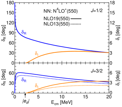
The lower panel of Fig. 3 represents the real and imaginary phase shifts in the $J=3/2$ channel for both NLO13 and NLO19 $YN$ interactions. Because the ¹S₀ $\Lambda$ N interaction is irrelevant for $J=3/2$ , the difference of the phase shifts between NLO13 and NLO represents different properties of the ³S₁ part of these interactions, despite the almost identical phase shifts of the ³S₁ phase shifts shown in Fig. 2. The behavior of the phase shifts corresponds to the absence of a bound state in this channel. The enhancement of the cross-section at low energies, however, implies the presence of a pole close to the axis. The position of the virtual state is approximated by the effective range parameters as HYO13

k=\frac{i}{r_{e}}-\frac{1}{r_{e}}\sqrt{\frac{2r_{e}}{a_{s}}-1}=\frac{i}{r_{e}}\left(1-\sqrt{1-\frac{2r_{e}}{a_{s}}}\right),

(12)

where $a_{s}$ is a scattering length and $r_{e}$ is an effective range, respectively. The effective range parameters deduced from the calculated phase shifts are discussed in the following section. By assigning the values given in Table I in the following section, the momentum $k$ becomes $-0.079i$ for NLO13 and $-0.051i$ for NLO19. The corresponding energy $E=\frac{\hbar^{2}}{2\mu_{\Lambda d}}k^{2}$ , where $\mu_{\Lambda d}$ is a $\Lambda d$ reduced mass, is $-0.17$ MeV for NLO13 and $-0.072$ MeV for NLO19.

It is noted that the imaginary part of the calculated phase shifts is small in both $J=1/2$ and $J=3/2$ , which relates to the fact that the ${}^{1}S_{0}$ channel is not allowed in the final state.

III.2 $\Lambda d$ effective range parameters

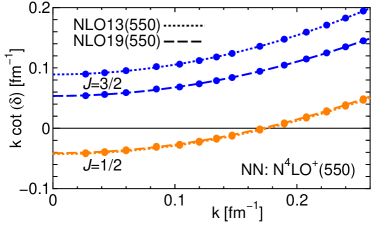
We estimate scattering length and effective range parameters by fitting the calculated phase shifts, $k\cot\delta$ below the deuteron breakup threshold, by a function $c_{0}+c_{1}k^{2}+c_{2}k^{4}$ . Figure 4 depicts the fit. Table 1 tabulates the results of the scattering length $a_{s}=-1/c_{0}$ and the effective range $r_{e}=2c_{1}$ . It is noted that these values are comparable to those of the preliminary results from the measurement in heavy-ion collisions in Ref. HU24 : $a_{s}^{J=1/2}=20_{-3}^{+3}$ fm, $r_{e}^{J=1/2}=3_{-1}^{+2}$ fm and $a_{s}^{J=3/2}=-16_{-1}^{+2}$ fm, $r_{e}^{J=3/2}=2_{-1}^{+1}$ fm.

The effective range parameters in the channel that bears a bound state are related to the separation energy $B_{\Lambda}$ by a Bethe formula BETH49 , which gives

B_{\Lambda}=\frac{\hbar^{2}}{\mu_{\Lambda d}r_{e}^{2}}\left\{1-\frac{r_{e}}{a_{s}}-\sqrt{1-\frac{2r_{e}}{a_{s}}}\right\}.

(13)

Using the values in Table 1, the expected $B_{\Lambda}$ becomes $57.9$ keV for NLO13 and $53.3$ keV for NLO19. The Faddeev calculations KKM23 for the bound hypertriton with the same $NN$ and $YN$ interactions predict $B_{\Lambda}=79$ keV for NLO13 and $B_{\Lambda}=87$ keV for NLO19. The magnitude of the difference is small but not negligible compared to the small value of $B_{\Lambda}$ . There are several sources of the difference. The bound-state calculation in Ref. KKM23 explicitly includes a $\Sigma NN$ component. However, the $\Sigma NN$ component is disregarded in the present scattering calculation, though the $\Lambda N$ - $\Sigma N$ coupling is taken care of in calculating the $\Lambda N$ $t$ matrix. In addition, higher partial waves are included in the Faddeev three-body calculations. It is noteworthy that the hypertriton separation energy obtained by Faddeev calculations with ignoring the $\Sigma$ and higher partial waves in Faddeev components is 73 keV for NLO13 and 76 keV for NLO19. These values are closer to the estimates derived from the Bethe formula. The remaining discrepancy may be attributed to the rearrangement effect of the deuteron wave function in forming the hypertriton bound state.

total spin	$YN$ int.	$a_{s}$ (fm)	$r_{e}$ (fm)
$J=1/2$	NLO13	$\phantom{-}23.4$	2.77
	NLO19	$\phantom{-}24.3$	2.80
$J=3/2$	NLO13	$-11.2$	3.25
	NLO19	$-18.7$	2.87

Table 1: Scattering length and effective range parameters deduced from the fit of the calculated phase shift presented in Fig. 4.

III.3 $\Lambda d$ correlation function

Explicit data from $\Lambda$ -deuteron scattering experiments are not available. An alternative way to probe the feature of the $\Lambda$ d interaction has been developed in heavy-ion collision experiments by measurement of $\Lambda$ d correlations . The $\Lambda$ d momentum correlation function measured in experiments corresponds to the following quantity FAB21 ; OMMH16 :

C_{\Lambda d}^{J}(k)=1+4\pi\int_{0}^{\infty}r^{2}dr\;S_{12}(r)\{|\psi_{J}(k;r)|^{2}-|j_{0}(kr)|^{2}\},

(14)

where $j_{0}(kr)$ is a spherical Bessel function, and $\psi_{J}(k;r)$ is a $\Lambda$ d scattering wave function in the channel with the total spin of $J$ . $S_{12}(r)$ is a source function that is assumed to be a conventional Gaussian form with a range parameter $R$ ,

S_{12}(r)=\frac{1}{(2\sqrt{\pi}R)^{3}}\exp(-\frac{1}{4R^{2}}r^{2}).

(15)

The $\Lambda$ d wave function in coordinate space is constructed from half-off-shell $T$ matrices obtained by solving the Faddeev equation. The explicit expression is explained in Appendix C. Realistic calculations of the correlation function taking into account the three-body dynamics that the Faddeev wave functions yield is a future subject.

The total spin is unseparated in experiments. Therefore, the following spin-averaged quantity is relevant when a comparison with the experimental data is made.

C_{\Lambda d}(k)=\frac{1}{3}C_{\Lambda d}^{J=1/2}(k)+\frac{2}{3}C_{\Lambda d}^{J=3/2}(k).

(16)

Figure 5 displays the spin-averaged results of the NNLO13 and NNLO19 $YN$ interactions with the $NN$ interaction of N⁴LO⁺. The selection of the range parameter, $R=1.2$ , 2.5, and 5 fm, follows that of Ref. HAID20 . The difference between the results of NLO13 and NLO19 comes from $C_{\Lambda d}^{J=3/2}$ .

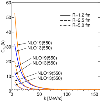
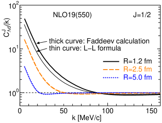
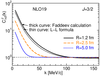
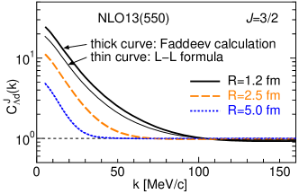
The individual momentum correlation function for $J=1/2$ and $J=3/2$ are shown in Fig. 6 on a vertical logarithmic scale. The upper panel represents the correlation function for $J=1/2$ , in which only the results of NLO19 are depicted because NLO13 and NLO19 provide almost the same results as is expected from the indistinguishability in the phase shifts, The lower two panels show the result for $J=3/2$ . In this case, the correlation function of NLO19 is $2\sim 3$ times larger than that of NLO13. Because the magnitude and weight of the $C_{\Lambda d}^{J=3/2}$ in which only the ³S₁ $\Lambda$ N interaction is relevant are larger than those of $C_{\Lambda d}^{J=1/2}$ , the experimental data can provide valuable information about the relative strength of the ¹S₀ and ³S₁ $\Lambda$ N interactions.

The theoretical correlation function $C_{\Lambda d}^{J}$ has been approximated by the following expression, which has been referred to as the Lednický-Lyuboshitz LL82 model formula:

	$\displaystyle C_{\Lambda d}^{J}\approx$	$\displaystyle\;1+\frac{\|f_{J}(k)\|^{2}}{2R}F(r_{e})+\frac{2\mbox{Re}f_{J}(k)}{\sqrt{\pi}R}F_{1}(x)$
		$\displaystyle-\frac{\mbox{Im}f_{J}(k)}{R}F_{2}(x),$		(17)

where $f_{J}$ is the scattering amplitude, $R$ is the range parameter, and $x\equiv 2kR$ . Three functions, i.e., $F$ , $F_{1}$ , and $F_{2}$ , are given by $F(r_{e})=1-r_{e}/(2\sqrt{\pi}R)$ , $F_{1}(x)=\int_{0}^{x}dt\>e^{t^{2}-x^{2}}/x$ , and $F_{2}(x)=(1-e^{-x^{2}})/x$ . When $f_{J}$ is approximated by the effective range parameters as

	$\displaystyle f_{J}=$	$\displaystyle\frac{e^{2i\delta_{J}}-1}{2ik}=\frac{1}{k\cot\delta_{J}-ik}$
	$\displaystyle\approx$	$\displaystyle\frac{1}{-\frac{1}{a_{s}}+\frac{1}{2}r_{e}k^{2}-ik}.$		(18)

$C_{\Lambda d}^{J}$ is estimated by giving $R$ , $a_{s}$ , and $r_{e}$ . It is instructive to evaluate the approximated $C_{\Lambda d}^{J}$ using the effective range parameters tabulated in Table 1 and compare it with the correlation function obtained by the $\Lambda$ d relative wave function from the Faddeev calculation.

The thick curves in Fig. 6 are the results of the Faddeev calculations on a vertical logarithmic scale. The thin curve depicts the correlation functions obtained by the effective range parameters. Except for $R=1.2$ fm, the thick and thin curves are overlapping and indistinguishable. The difference between the two curves in the case of $R=1.2$ fm is also small. This result indicates that the approximation of the correlation function by Eq. (17) is dependable.

IV Summary

We describe $\Lambda$ -deuteron elastic scattering in a Faddeev formulation for low energies, up to 20 MeV, crossing the deuteron breakup threshold. Although direct measurements of the scattering are not currently feasible, experimental information is included in correlation functions that can be accessed through heavy-ion collision measurements. The preliminary results were recently reported in Ref. HU24 . The calculated phase shifts are a valuable feature that elucidates the properties of the underlying $YN$ interactions that are employed, including the effect of the relative strength of the spin singlet and triplet parts in a few-body system. It is also meaningful to investigate the implication of different parametrizations of the $YN$ interactions in the scattering process of the $\Lambda$ hyperon on the deuteron.

The numerical evaluation is more complex than that of nucleon-deuteron scattering due to the mass difference between the $\Lambda$ hyperon and the nucleon. For the sake of completeness, an outline of the treatment of a deuteron pole and a moving singularity is provided in Appendices A $-$ C.

Based on the half-off-shell $t$ matrices obtained by solving the Faddeev equation, $\Lambda d$ relative wave functions are constructed, and momentum space $\Lambda d$ correlation functions are evaluated. The evaluated correlation functions demonstrate the efficiency of the approximated expression, given by Eq. (17), although a slight deviation is observed when the source radius is small. In Ref. MHS23 , the $\Lambda p$ correlation data are employed to constrain parametrizing $\Lambda N$ interactions. The $\Lambda d$ correlation data can provide additional constraints through the use of Faddeev calculations.

Finally, it is noted that the present method can be straightforwardly applied to $\Xi d$ scattering, which could help in studying the properties of $\Xi N$ interactions.

Acknowledgments. We are grateful to K. Miyagawa for his valuable discussions and comments on this work. This work is supported by JSPS KAKENHI Grants No. JP19K03849 and No. JP22K03597.

Appendix A Explicit equations in partial wave expansion

Explicit equations in a partial wave expansion of Eqs. (6) and (7) are derived. We follow the notation for the partial wave project state in Ref. GL96 .

	$\displaystyle\langle\mbox{\boldmath$p$}^{\prime}\|plm\rangle=\frac{\delta(p^{\prime}-p)}{p^{\prime}p}Y_{\ell m}(\hat{\mbox{\boldmath$p$}^{\prime}}),\hskip 20.00003pt\|p(ls)jm\rangle=\sum_{\mu}(\ell\mu sm-\mu\|jm)\|plm\rangle\|sm-\mu\rangle,$		(19)
	$\displaystyle\mbox{3-body state}\hskip 5.0pt\|pq\alpha\rangle=\|pq(\ell s)j(\lambda 1/2)I(jI)JM(t1/2)TM_{T}\rangle,$		(20)
	$\displaystyle\langle p^{\prime}q^{\prime}\alpha^{\prime}\|pq\alpha\rangle=\frac{\delta(q^{\prime}-q)}{q^{\prime}q}\frac{\delta(p^{\prime}-p)}{p^{\prime}p}\delta_{\alpha^{\prime}\alpha},\hskip 20.00003pt\sum_{\alpha}\int_{0}^{\infty}p^{2}dp\int_{0}^{\infty}q^{2}dq\;\|pq\alpha\rangle\langle pq\alpha\|=I,$		(21)

where $Y_{\ell m}$ stands for a spherical harmonics and $(\ell\mu sm-\mu|jm)$ represents a Clebsch-Gordan coefficient. Inserting the identity operator, Eqs. (6) and (7) read

$\displaystyle\langle p_{3}q_{3}\alpha_{3}\|T_{3}\|\phi\rangle=$	$\displaystyle 2\sum_{\alpha_{3}^{\prime}}\int_{0}^{\infty}{p_{3}^{\prime}}^{2}dp_{3}^{\prime}\int_{0}^{\infty}{q_{3}^{\prime}}^{2}dq_{3}^{\prime}\sum_{\alpha_{2}^{\prime}}\int_{0}^{\infty}{p_{2}^{\prime}}^{2}dp_{2}^{\prime}\int_{0}^{\infty}{q_{2}^{\prime}}^{2}dq_{2}^{\prime}$
	$\displaystyle\times\langle p_{3}q_{3}\alpha_{3}\|t_{3}G_{0}\|p_{3}^{\prime}q_{3}^{\prime}\alpha_{3}^{\prime}\rangle\langle p_{3}^{\prime}q_{3}^{\prime}\alpha_{3}^{\prime}\|p_{2}^{\prime}q_{2}^{\prime}\alpha_{2}^{\prime}\rangle\langle p_{2}^{\prime}q_{2}^{\prime}\alpha_{2}^{\prime}\|T_{2}\|\phi\rangle,$	(22)
$\displaystyle\langle p_{2}q_{2}\alpha_{2}\|T_{2}\|\phi\rangle=$	$\displaystyle\sum_{\alpha_{2}^{\prime}}\int_{0}^{\infty}{p_{2}^{\prime}}^{2}dp_{2}^{\prime}\int_{0}^{\infty}{q_{2}^{\prime}}^{2}dq_{2}^{\prime}\sum_{\alpha_{3}^{\prime}}\int_{0}^{\infty}{p_{3}^{\prime}}^{2}dp_{3}^{\prime}\int_{0}^{\infty}{q_{3}^{\prime}}^{2}dq_{3}^{\prime}$
	$\displaystyle\times\left\{\langle p_{2}q_{2}\alpha_{2}\|t_{2}\|p_{2}^{\prime}q_{2}^{\prime}\alpha_{2}^{\prime}\rangle\langle p_{2}^{\prime}q_{2}^{\prime}\alpha_{2}^{\prime}\|p_{3}^{\prime}q_{3}^{\prime}\alpha_{3}^{\prime}\rangle\langle p_{3}^{\prime}q_{3}^{\prime}\alpha_{3}^{\prime}\|\phi\rangle\right.$
	$\displaystyle\left.+\langle p_{2}q_{2}\alpha_{2}\|t_{2}G_{0}\|p_{2}^{\prime}q_{2}^{\prime}\alpha_{2}^{\prime}\rangle\langle p_{2}^{\prime}q_{2}^{\prime}\alpha_{2}^{\prime}\|p_{3}^{\prime}q_{3}^{\prime}\alpha_{3}^{\prime}\rangle\langle p_{3}^{\prime}q_{3}^{\prime}\alpha_{3}^{\prime}\|T_{3}\|\phi\rangle\right\}$
$\displaystyle-$	$\displaystyle\sum_{\alpha_{2}^{\prime}}\int_{0}^{\infty}{p_{2}^{\prime}}^{2}dp_{2}^{\prime}\int_{0}^{\infty}{q_{2}^{\prime}}^{2}dq_{2}^{\prime}\sum_{\alpha_{2}^{\prime\prime}}\int_{0}^{\infty}{p_{2}^{\prime\prime}}^{2}dp_{2}^{\prime\prime}\int_{0}^{\infty}{q_{3}^{\prime\prime}}^{2}dq_{2}^{\prime\prime}$
	$\displaystyle\times\langle p_{2}q_{2}\alpha_{2}\|t_{2}\|p_{2}^{\prime}q_{2}^{\prime}\alpha_{2}^{\prime}\rangle\langle p_{2}^{\prime}q_{2}^{\prime}\alpha_{2}^{\prime}\|P_{12}G_{0}\|p_{2}^{\prime\prime}q_{2}^{\prime\prime}\alpha_{2}^{\prime\prime}\rangle\langle p_{2}^{\prime\prime}q_{2}^{\prime\prime}\alpha_{2}^{\prime\prime}\|T_{2}\|\phi\rangle,$	(23)

where the antisymmetric property of the state $\langle p_{2}^{\prime}q_{2}^{\prime}\alpha_{2}^{\prime}|$ under the $P_{12}$ operation is used.

The matrix elements of $t_{3}G_{0}$ , $t_{2}$ , and $t_{2}G_{0}$ are explicitly wriiten as

$\displaystyle\langle p_{3}q_{3}\alpha_{3}\|t_{3}G_{0}\|p_{3}^{\prime}q_{3}^{\prime}\alpha_{3}^{\prime}\rangle=$	$\displaystyle\frac{\delta(q_{3}-q_{3}^{\prime})}{q_{3}q_{3}^{\prime}}\langle p_{3}\alpha_{3}\|t_{3}(E-h_{\Lambda(NN)}(q_{3}))\|p_{3}^{\prime}\alpha_{3}^{\prime}\rangle\frac{1}{E-h_{NN}(p_{3}^{\prime})-h_{\Lambda(NN)}(q_{3})+i\epsilon},$	(24)
$\displaystyle\langle p_{2}q_{2}\alpha_{2}\|t_{2}\|p_{2}^{\prime}q_{2}^{\prime}\alpha_{2}^{\prime}\rangle=$	$\displaystyle\frac{\delta(q_{2}-q_{2}^{\prime})}{q_{2}q_{2}^{\prime}}\langle p_{2}\alpha_{2}\|t_{2}(E-h_{N(\Lambda N)}(q_{2}))\|p_{2}^{\prime}\alpha_{2}^{\prime}\rangle,$	(25)
$\displaystyle\langle p_{2}q_{2}\alpha_{3}\|t_{2}G_{0}\|p_{2}^{\prime}q_{2}^{\prime}\alpha_{2}^{\prime}\rangle=$	$\displaystyle\frac{\delta(q_{2}-q_{2}^{\prime})}{q_{2}q_{2}^{\prime}}\langle p_{2}\alpha_{2}\|t_{2}(E-h_{N(\Lambda N)}(q_{2}))\|p_{2}^{\prime}\alpha_{2}^{\prime}\rangle\frac{1}{E-h_{\Lambda N}(p_{2}^{\prime})-h_{N(\Lambda N)}(q_{2})+i\epsilon},$	(26)

where $h_{NN}(p_{3}^{\prime})=\frac{\hbar^{2}}{2\mu_{NN}}{p_{3}^{\prime}}^{2}$ with $\mu_{NN}=\frac{1}{2}m_{N}$ , $h_{\Lambda(NN)}(q_{3})=\frac{\hbar^{2}}{2\mu_{\Lambda(NN)}}q_{3}^{2}$ with $\mu_{\Lambda(NN)}=\frac{2m_{N}m_{\Lambda}}{2m_{N}+m_{\Lambda}}$ , $h_{\Lambda N}(p_{2}^{\prime})=\frac{\hbar^{2}}{2\mu_{\Lambda N}}{p_{2}^{\prime}}^{2}$ with $\mu_{N(\Lambda N)}=\frac{m_{N}m_{\Lambda}}{m_{N}+m_{\Lambda}}$ , and $h_{N(\Lambda N)}(q_{2})=\frac{\hbar^{2}}{2\mu_{N(\Lambda N)}}q_{2}^{2}$ with $\mu_{N(\Lambda N)}=\frac{m_{N}(m_{N}+m_{\Lambda})}{2m_{N}+m_{\Lambda}}$ . The matrix elements of the permutation of Jacobi momenta have the following form:

$\displaystyle\langle p_{3}^{\prime}q_{3}^{\prime}\alpha_{3}^{\prime}\|p_{2}^{\prime}q_{2}^{\prime}\alpha_{2}^{\prime}\rangle=$	$\displaystyle\int_{-1}^{1}d\cos\theta\;G_{\alpha_{3}^{\prime}\alpha_{2}^{\prime}}^{(2)}(q_{3}^{\prime},q_{2}^{\prime},\cos\theta)\frac{1}{{p_{3}^{\prime}}^{\ell_{\alpha_{3}^{\prime}}}{p_{2}^{\prime}}^{\ell_{\alpha_{2}^{\prime}}}}\frac{\delta(p_{3}^{\prime}-\pi_{3})\delta(p_{2}^{\prime}-\pi_{2})}{{p_{3}^{\prime}}^{2}{p_{2}^{\prime}}^{2}},$	(27)
$\displaystyle\langle p_{2}^{\prime}q_{2}^{\prime}\alpha_{2}^{\prime}\|p_{3}^{\prime}q_{3}^{\prime}\alpha_{3}^{\prime}\rangle=$	$\displaystyle\int_{-1}^{1}d\cos\theta\;G_{\alpha_{2}^{\prime}\alpha_{3}^{\prime}}^{(1)}(q_{2}^{\prime},q_{3}^{\prime},\cos\theta)\frac{1}{{p_{2}^{\prime}}^{\ell_{\alpha_{2}^{\prime}}}{p_{3}^{\prime}}^{\ell_{\alpha_{3}^{\prime}}}}\frac{\delta(p_{2}^{\prime}-\pi_{2}^{\prime})\delta(p_{3}^{\prime}-\pi_{3}^{\prime})}{{p_{2}^{\prime}}^{2}{p_{3}^{\prime}}^{2}},$	(28)
$\displaystyle\langle p_{2}^{\prime}q_{2}^{\prime}\alpha_{2}^{\prime}\|P_{12}G_{0}\|p_{2}^{\prime\prime}q_{2}^{\prime\prime}\alpha_{2}^{\prime\prime}\rangle=$	$\displaystyle\int_{-1}^{1}d\cos\theta\;G_{\alpha_{2}^{\prime}\alpha_{2}^{\prime\prime}}^{(3)}(q_{2}^{\prime},q_{2}^{\prime\prime},\cos\theta)\frac{1}{{p_{2}^{\prime}}^{\ell_{\alpha_{2}^{\prime}}}{p_{2}^{\prime\prime}}^{\ell_{\alpha_{2}^{\prime\prime}}}}\frac{\delta(p_{2}^{\prime}-\pi_{2}^{\prime\prime})\delta(p_{2}^{\prime\prime}-\pi_{2}^{\prime\prime\prime})}{{p_{2}^{\prime}}^{2}{p_{2}^{\prime\prime}}^{2}},$	(29)

where $\cos\theta=\cos\widehat{\mbox{\boldmath$q$}_{3}^{\prime}\mbox{\boldmath$q$}_{2}^{\prime}}$ in Eq. (A9), $\cos\theta=\cos\widehat{\mbox{\boldmath$q$}_{2}^{\prime}\mbox{\boldmath$q$}_{3}^{\prime}}$ in Eq. (A10), and $\cos\theta=\cos\widehat{\mbox{\boldmath$q$}_{2}^{\prime}\mbox{\boldmath$q$}_{2}^{\prime\prime}}$ in Eq. (A11), respectively. Various momenta in the above equations are defined as follows:

$\displaystyle\pi_{3}=$	$\displaystyle[q_{2}^{\prime 2}+r_{NN}^{2}{q_{3}}^{2}+2r_{NN}q_{2}^{\prime}q_{3}^{\prime}\cos\theta]^{1/2},$	$\displaystyle\pi_{2}=[{q_{3}}^{2}+r_{\Lambda N}^{2}q_{2}^{\prime 2}+2r_{\Lambda N}q_{2}^{\prime}q_{3}^{\prime}\cos\theta]^{1/2},$
$\displaystyle\pi_{30}=$	$\displaystyle[q_{2}^{\prime 2}+r_{NN}^{2}q_{0}^{2}+2r_{NN}q_{2}^{\prime}q_{0}\cos\theta]^{1/2},$	$\displaystyle\pi_{20}=[{q_{0}}^{2}+r_{\Lambda N}^{2}q_{2}^{\prime 2}+2r_{\Lambda N}q_{2}^{\prime}q_{0}\cos\theta]^{1/2},$
$\displaystyle\pi_{3}^{\prime}=$	$\displaystyle[q_{2}^{2}+r_{NN}^{2}{q_{3}^{\prime}}^{2}+2r_{NN}q_{2}q_{3}^{\prime}\cos\theta]^{1/2},$	$\displaystyle\pi_{2}^{\prime}=[{q_{3}^{\prime}}^{2}+r_{\Lambda N}^{2}q_{2}^{2}+2r_{\Lambda N}q_{2}q_{3}^{\prime}\cos\theta]^{1/2},$
$\displaystyle\pi_{2}^{\prime\prime}=$	$\displaystyle[q_{2}^{\prime\prime 2}+r_{N\Lambda}^{2}q_{2}^{2}+2r_{N\Lambda}q_{2}q_{2}^{\prime\prime}\cos\theta]^{1/2},$	$\displaystyle\pi_{2}^{\prime\prime\prime}=[q_{2}^{2}+r_{N\Lambda}^{2}q_{2}^{\prime\prime 2}+2r_{N\Lambda}q_{2}q_{2}^{\prime\prime}\cos\theta]^{1/2},$
$\displaystyle\pi_{30}^{\prime}=$	$\displaystyle[q_{2}^{2}+r_{NN}^{2}q_{0}^{2}+2r_{NN}q_{2}q_{0}\cos\theta]^{1/2},$	$\displaystyle\pi_{20}^{\prime}=[{q_{0}}^{2}+r_{\Lambda N}^{2}q_{2}^{2}+2r_{\Lambda N}q_{2}q_{0}\cos\theta]^{1/2},$
$\displaystyle\pi_{3i}^{\prime}=$	$\displaystyle[{q_{2}}^{2}+r_{NN}^{2}q_{i}^{2}+2r_{NN}q_{2}q_{i}\cos\theta]^{1/2},$	$\displaystyle\pi_{2i}^{\prime}=[{q_{i}}^{2}+r_{\Lambda N}^{2}q_{2}^{2}+2r_{\Lambda N}q_{2}q_{i}\cos\theta]^{1/2},$	(30)

where $r_{NN}=\frac{1}{2}$ , $r_{N\Lambda}=\frac{m_{N}}{m_{N}+m_{\Lambda}}$ , and $r_{\Lambda N}=\frac{m_{\Lambda}}{m_{N}+m_{\Lambda}}$ , respectively. Before transforming Eqs. (A4) and (A5) further, it is necessary to explain the treatment of the deuteron pole in the $NN$ $t$ matrix.

Appendix B Treatment of deuteron pole

In the Faddeev equation, the $NN$ $t$ matrix depends on the momentum $q_{3}$ of the third particle $\Lambda$ .

t(q_{3})=v+v\frac{1}{E-h_{\Lambda(NN)}(q_{3})-h_{NN}(p_{3})+i\epsilon}t(q_{3})=v+v\frac{1}{E-h_{\Lambda(NN)}(q_{3})-h_{NN}(p_{3})-v+i\epsilon}v,

(31)

where $E$ is the total energy, and $v$ is a two-body $NN$ interaction. It is helpful to introduce a spectral decomposition to investigate the structure of the $t$ matrix. Assuming that there is one bound state $|d\rangle$ with its energy $-|e_{d}|$ for the Hamiltonian $H=\frac{\hbar^{2}}{2\mu_{NN}}p_{3}^{2}+v$ and denoting the eigenstate in the continuum with its momentum $k$ by $|\psi(\mbox{\boldmath$k$})\rangle$ , the completeness relation reads

\displaystyle\int\frac{d\mbox{\boldmath$k$}}{(2\pi)^{3}}|\psi(\mbox{\boldmath$k$})\rangle\langle\psi(\mbox{\boldmath$k$})|+|d\rangle\langle d|.

(32)

By inserting this relation into Eq. (31), the following expression is obtained.

\displaystyle t(q_{3})=

\displaystyle v+\int\frac{d\mbox{\boldmath$k$}}{(2\pi)^{3}}\frac{v|\psi(\mbox{\boldmath$k$})\rangle\langle\psi(\mbox{\boldmath$k$})|v}{E-h_{\Lambda(NN)}(q_{3})-h_{NN}(k)-v+i\epsilon}+\frac{v|d\rangle\langle d|v}{E-h_{\Lambda(NN)}(q_{3})+|e_{d}|+i\epsilon}.

(33)

The $t$ matrix is solved numerically. The expression of Eq. (33) is used for the prescription to treat the singularity at the deuteron pole position. The denominator of the second term has a pole for the momentum $k$ when $E-h_{\Lambda(NN)}(q_{3})>0$ . This feature is known as a moving pole. The third term of Eq. (33) has a pole that appears in the $t$ matrix of the deuteron channel when $E_{cm}\equiv E+|e_{d}|>0$ . The singularity is written as

\frac{v|d\rangle\langle d|v}{E-h_{\Lambda(NN)}(q_{3})+|e_{d}|+i\epsilon}=\mbox{P}\frac{v|d\rangle\langle d|v}{E-h_{\Lambda(NN)}(q_{3})+|e_{d}|+i\epsilon}-i\pi\delta(E-h_{\Lambda(NN)}(q_{3})+|e_{d}|)v|d\rangle\langle d|v.

(34)

Because the $t$ -matrix solved numerically does not contain the $\delta$ -function part, it has to be added separately as in Ref. FF10 . The $\delta$ -function part can be written as follows:

-i\pi\delta(E-h_{\Lambda(NN)}(q_{3})+|e_{d}|)v|\;d\rangle\langle d|v=-i\frac{\pi}{2q_{0}}\frac{2\mu_{\Lambda(NN)}}{\hbar^{2}}\delta(q_{3}-q_{0})v|d\rangle\langle d|v,

(35)

where $q_{0}$ defined by $E+|e_{d}|\equiv\frac{\hbar^{2}}{2\mu_{\Lambda(NN)}}q_{0}^{2}$ is introduced.

It is convenient to treat the $\delta$ -function part separately in the set of Faddeev equations. Because the bound-state wave function is known, and $\langle p_{3}|v|d\rangle=\left\{e_{d}-2\frac{\hbar^{2}}{\mu_{NN}}p_{3}^{2}\right\}\langle p_{3}|d\rangle$ , the matrix element of the numerator of the third term is rewritten as follows:

\displaystyle\langle p_{3}|v|d\rangle\langle d|v|p_{3}^{\prime}\rangle=\left\{e_{d}-\frac{\hbar^{2}}{2\mu_{NN}}p_{3}^{2}\right\}\left\{e_{d}-\frac{\hbar^{2}}{2\mu_{NN}}{p_{3}^{\prime}}^{2}\right\}\langle p_{3}|d\rangle\langle d|p_{3}^{\prime}\rangle,

(36)

where $\langle p_{3}|d\rangle$ is a bound-state (deuteron) wave function in momentum space.

It is convenient to separate the contribution of the $\delta$ -function part of Eq. (34) and express $T_{3}$ as $T_{3}=T_{3}^{R}+iT_{3}^{I}$ . It is noted that both $T_{3}^{R}$ and $T_{3}^{I}$ are complex. Then, Eqs. (A4) and (A5) are expressed as follows.

$\displaystyle\langle p_{3}q_{3}\alpha_{3}\|T_{3}^{R}\|\phi\rangle=$	$\displaystyle 2\sum_{\alpha_{3}^{\prime}}\sum_{\alpha_{2}^{\prime}}\int q_{2}^{\prime 2}dq_{2}^{\prime}\int_{-1}^{1}d\cos\theta\langle p_{3}\alpha_{3^{\prime}}\|t_{3}(E-h_{\Lambda(NN)}(q_{3}))\|\pi_{3}\alpha_{3}^{\prime}\rangle\frac{1}{E-h_{NN}(\pi_{3})-h_{\Lambda(NN)}(q_{3})+i\epsilon}$
	$\displaystyle\times G_{\alpha_{3}^{\prime}\alpha_{2}^{\prime}}^{(2)}(q_{3},q_{2}^{\prime},\cos\theta)\frac{1}{{\pi_{3}}^{\ell_{\alpha_{3}^{\prime}}}{\pi_{2}}^{\ell_{\alpha_{2}^{\prime}}}}\langle\pi_{2}q_{2}^{\prime}\alpha_{2}^{\prime}\|T_{2}\|\phi\rangle,$	(37)
$\displaystyle\langle p_{3}q_{0}\alpha_{3}\|T_{3}^{I}\|\phi\rangle=$	$\displaystyle-\delta_{\alpha_{3}\alpha_{d}}\left(\epsilon_{d}-h_{NN}(p_{3})\right)\frac{2\mu_{\Lambda(NN)}}{\hbar^{2}}\pi q_{0}\sum_{\alpha_{d}^{\prime}}\sum_{\alpha_{2}^{\prime}}\int q_{2}^{\prime 2}dq_{2}^{\prime}\int_{-1}^{1}d\cos\theta\;\langle p_{3}\alpha_{d}\|\psi_{d}\rangle\langle\psi_{d}\|\pi_{30}\alpha_{d}^{\prime}\rangle$
	$\displaystyle\times G_{\alpha_{3}^{\prime}\alpha_{2}^{\prime}}^{(2)}(q_{0},q_{2}^{\prime},\cos\theta)\frac{1}{{\pi_{30}}^{\ell_{\alpha_{3}^{\prime}}}{\pi_{20}}^{\ell_{\alpha_{2}^{\prime}}}}\langle\pi_{20}{q_{2}}^{\prime}\alpha_{2}^{\prime}\|T_{2}\|\phi\rangle,$	(38)
$\displaystyle\langle p_{2}q_{2}\alpha_{2}\|T_{2}\|\phi\rangle=$	$\displaystyle\sum_{\alpha_{2}^{\prime}}\sum_{\alpha_{d}^{\prime}}\int_{-1}^{1}d\cos\theta\langle p_{2}\alpha_{2}\|t_{2}\|\pi_{2i}^{\prime}\alpha_{2i}^{\prime}\rangle\;G_{\alpha_{2}^{\prime}\alpha_{d}^{\prime}}^{(1)}(q_{2},q_{i},\cos\theta)\frac{1}{{\pi_{2i}^{\prime}}^{\ell_{\alpha_{2}^{\prime}}}{\pi_{3i}^{\prime}}^{\ell_{\alpha_{d}^{\prime}}}}\langle\pi_{3i}^{\prime}\alpha_{d}^{\prime}\|\psi_{d}\rangle$
$\displaystyle+$	$\displaystyle\sum_{\alpha_{2}^{\prime}}\sum_{\alpha_{3}^{\prime}}\int q_{3}^{\prime 2}dq_{3}^{\prime}\int_{-1}^{1}d\cos\theta\;\langle p_{2}\alpha_{2}\|t_{2}\|\pi_{2}^{\prime}\alpha_{2}^{\prime}\rangle\;\frac{1}{E-h_{\Lambda N}(\pi_{2}^{\prime})-\frac{\hbar^{2}}{2\mu_{N(\Lambda N)}}q_{2}^{2}+i\epsilon}$
	$\displaystyle\times G_{\alpha_{2}^{\prime}\alpha_{3}^{\prime}}^{(1)}(q_{2},q_{3}^{\prime},\cos\theta)\frac{1}{{\pi_{2}^{\prime}}^{\ell_{\alpha_{2}^{\prime}}}{\pi_{3}^{\prime}}^{\ell_{\alpha_{3}^{\prime}}}}\langle\pi_{3}^{\prime}q_{3}^{\prime}\alpha_{3}^{\prime}\|T_{3}^{R}\|\phi\rangle$
$\displaystyle+$	$\displaystyle i\sum_{\alpha_{2}^{\prime}}\sum_{\alpha_{d}}\int_{-1}^{1}d\cos\theta\;\langle p_{2}\alpha_{2}\|t_{2}\|\pi_{20}^{\prime}\alpha_{2}^{\prime}\rangle G_{\alpha_{2}^{\prime}\alpha_{3}^{\prime}}^{(1)}(q_{2},q_{0},\cos\theta)\frac{1}{{\pi_{20}^{\prime}}^{\ell_{\alpha_{2}^{\prime}}}{\pi_{30}^{\prime}}^{\ell_{\alpha_{3}^{\prime}}}}\langle\pi_{30}^{\prime}q_{0}\alpha_{3}^{\prime}\|\tilde{T}_{3}^{I}\|\phi\rangle$
$\displaystyle-$	$\displaystyle\sum_{\alpha_{2}^{\prime}}\sum_{\alpha_{2}^{\prime\prime}}\int q_{2}^{\prime\prime 2}dq_{2}^{\prime\prime}\int_{-1}^{1}d\cos\theta\;\langle p_{2}\alpha_{2}\|t_{2}\|\pi_{2}^{\prime\prime}\alpha_{2}^{\prime}\rangle\;G_{\alpha_{2}^{\prime}\alpha_{2}^{\prime\prime}}^{(3)}(q_{2},q_{2}^{\prime\prime},\cos\theta)\frac{1}{{\pi_{2}^{\prime\prime}}^{\ell_{\alpha_{2}^{\prime}}}{\pi_{2}^{\prime\prime\prime}}^{\ell_{\alpha_{2}^{\prime\prime}}}}$
	$\displaystyle\times\frac{1}{E-h_{\Lambda N}(\pi_{2}^{\prime\prime\prime})-h_{N(\Lambda N)}(q_{2}^{\prime\prime})+i\epsilon}\langle\pi_{2}^{\prime\prime\prime}q_{2}^{\prime\prime}\alpha_{2}^{\prime\prime}\|T_{2}\|\phi\rangle,$	(39)

In Eq. (B7), $\langle p_{3}\alpha_{3^{\prime}}|t_{3}(E-h_{\Lambda(NN)}(q_{3}))|\pi_{3}\alpha_{3}^{\prime}\rangle$ in the deuteron channel is understood as

\langle p_{3}|t_{3}(E-h_{\Lambda(NN)}(q_{3}))|\pi_{3}\rangle-\frac{2\mu_{\Lambda(NN)}}{\hbar^{2}}\frac{\langle p_{3}|v|d\rangle\langle d|v|\pi_{3}\rangle}{q_{0}^{2}-q_{3}^{2}}+\mbox{P}\frac{2\mu_{\Lambda(NN)}}{\hbar^{2}}\frac{\langle p_{3}|v|d\rangle\langle d|v|\pi_{3}\rangle}{q_{0}^{2}-q_{3}^{2}}.

(40)

The divergent behavior of the $t_{3}$ -matrix element around the pole position is removed by the second term. When $T_{3}^{R}$ is inserted in Eq. (B9), the principal value of $q_{3}^{\prime}$ integration is treated by the standard subtraction method.

When $E=E_{cm}+e_{d}>0$ , there is a notorious problem of moving singularities GL96 in which logarithmic singularities appear. We use numerical techniques in the literature FF10 ; LIU05 , but the actual calculations become intricate because of the mass difference between the $\Lambda$ hyperon and the nucleon.

Appendix C Crescent area and logarithmic singularity

Three different types of the crescent area in which the logarithmic singularity associated with the so-called moving pole of the Green function exists in the case of $E=E_{cm}+e_{d}>0$ appear, which are depicted in Fig. 7. Various reference points shown in these figures are defined as follows:

$\displaystyle q_{2,m}^{\prime}=$	$\displaystyle q_{2,m}=\sqrt{\frac{2\mu_{N(\Lambda N)}}{\hbar^{2}}E},\hskip 10.00002ptq_{2,z}^{\prime}=q_{2,az}=\sqrt{\frac{2\mu_{NN}}{\hbar^{2}}E},\hskip 10.00002ptq_{2,t}^{\prime}=q_{2,at}=\sqrt{\frac{\mu_{N(\Lambda N)}}{\hbar^{2}}Er_{\Lambda N}}=r_{NN}\sqrt{\frac{2\mu_{\Lambda(NN)}}{\hbar^{2}}E},$
$\displaystyle q_{3,m}=$	$\displaystyle q_{3,am}^{\prime}=\sqrt{\frac{2\mu_{\Lambda(NN)}}{\hbar^{2}}E},\hskip 10.00002ptq_{3,z}=q_{3,az}^{\prime}=q_{2,bz}^{\prime}=q_{2,bz}=\sqrt{\frac{2\mu_{\Lambda N}}{\hbar^{2}}E},\hskip 10.00002ptq_{3,t}=\sqrt{\frac{\mu_{\Lambda(NN)}}{\hbar^{2}}Er_{\Lambda N}},$
$\displaystyle q_{3,at}^{\prime}=$	$\displaystyle\sqrt{\frac{\mu_{\Lambda(NN)}}{\hbar^{2}}Er_{\Lambda N}}=r_{\Lambda N}\sqrt{\frac{2\mu_{N(\Lambda N)}}{\hbar^{2}}E},\hskip 10.00002ptq_{2,bt}^{\prime}=q_{2,bt}=r_{N\Lambda}\sqrt{\frac{2\mu_{N(\Lambda N)}}{\hbar^{2}}E}.$	(41)

The mesh points for the $q_{3}$ momentum are set by separating them into the following three intervals:

[0,q_{3,t}],[q_{3,t},q_{3,z}],[q_{3,z},q_{3,m}].

(42)

Because of $q_{2,at}\neq q_{2,bt}$ and $q_{2,az}\neq q_{2,bz}$ , the mesh points for the $q_{2}$ momentum are set by separating them into the following five intervals:

[0,q_{2,bt}],[q_{2,bt},q_{2,at}],[q_{2,at},q_{2,az}],[q_{2,az},q_{2,bz}],[q_{2,bz},q_{2,m}].

(43)

The mesh points near $q_{2,m}$ , $q_{2,az}$ , and $q_{2,bz}$ are prepared by changing the variable to $\sqrt{q_{2,m}^{2}-q_{2}^{2}}$ etc. The Gauss-Legendre quadrature is used in each interval. The sufficiently fine mesh points are prepared around the deuteron pole $q_{0}$ that is larger $q_{3,m}$ . In solving Eqs. (A7) $-$ (A9), the momenta given in (30), in general, do not coincide with the prepared mesh points. This problem is circumvented by the technique of using a cubic Spline interpolation. The notorious logarithmic singularities in the crescent area are treated by the method described in detail in Refs. FF10 and LIU05 .

Appendix D $\Lambda$ -deuteron wave function in $r$ -space

Half-off-shell $T_{2}$ matrices in Eq. (7) determine the $\Lambda d$ relative wave function in $r$ space. A partial wave component is obtained by

\psi_{k,\ell}^{+}(r)=j_{\ell}(kr)+\frac{2\mu_{\Lambda d}}{\hbar^{2}}\int_{0}^{\infty}k^{\prime 2}dk^{\prime}\;\frac{j_{\ell}(k^{\prime}r)T_{2,\ell}(k^{\prime},k)}{k^{2}+i\epsilon-k^{\prime 2}},

(44)

where the tensor coupling is suppressed for simplicity. The integration is evaluated numerically by using a subtraction prescription,

\int_{0}^{\infty}k^{\prime 2}dk^{\prime}\;\frac{j_{\ell}(k^{\prime}r)T_{2,\ell(k^{\prime},k)}}{k^{2}+i\epsilon-k^{\prime 2}}=\int_{0}^{\infty}dk^{\prime}\frac{k^{\prime 2}j_{\ell}(k^{\prime}r)T_{2,\ell(k^{\prime},k)}-k^{2}j_{\ell}(kr)T_{2,\ell(k,k)}}{k^{2}-k^{\prime 2}}-i\frac{\pi k}{2}j_{\ell}(kr)T_{2,\ell}(k,k).

(45)

References

(1) H. Tamura, ”Overview of hypernuclear and strange particle physics - Experimental summary of HYP2022”, EPJ Web Conf. 271, 12001 (2022).
(2) P. Eckert, S. Ries, and P. Achenbach, Chart of hypernucleids - Hypernuclear Structure and Decay Data, 2023, https://hypernuclei.kph.uni-mainz.de/(unpublished).
(3) M. Kohno, H. Kamada, and K. Miyagawa, ”Contributions of 2 $\pi$ exchange, 1 $\pi$ exchange, and contact three-body forces in NNLO chiral effective field theory to ${}_{\Lambda}^{3}$ H”, Phys. Rev. C 106, 054004 (2022); 110, 019908(E) (2024).
(4) H. Garcilazo, T. Fernández-Caramés, and A. Valcarce, ” $\Lambda NN$ and $\Sigma NN$ systems at threshold”, Phys. Rev. C 75, 034002 (2007).
(5) H. Garcilazo, A. Valcarce, and T. Fernández-Caramés, ” $\Lambda NN$ and $\Sigma NN$ systems at threshold. II. The effect of $D$ waves”, Phys. Rev. C 76, 034001 (2007).
(6) H.-W. Hammer, ”The hypernuclei in effective field theory,” Nucl. Phys. A705, 173 (2002).
(7) F. Hildenbrand and H.-W. Hammer, ”Three-body hypernuclei in pionless effective field theory,” Phys. Rev. C 100, 034002 (2019).
(8) M. Schäfer, B. Bazak, N. Barnea, A. Gal, and J. Mareš, ”The continuum spectrum of hypernucler trios”, Phys. Rev. C 105, 015202 (2022).
(9) L. Fabbietti, V. Mantovani Sarti, and O. Vázquez Doce, ”Study of the Strong Interaction Among Hadrons with Correlations at the LHC”, Annu. Rev. Nucl. Part. Sci. 71, 377 (2021).
(10) Y. Hu (STAR collaboration), Measurement of $p$ - $\Lambda$ and $d$ - $\Lambda$ correlations in 3GeV Au+Au collisions at STAR, EPJ WEB Conf. 296, 14010 (2024).
(11) J. Haidenbauer, Exploring the $\Lambda$ -deuteron interaction via correlations in heavy-ion collisions, Phys. Rev. C 102, 034001 (2020).
(12) R. Lednický and V.L. Lyuboshitz, Final State Interaction Effect on Pairing Correlations Between Particles with Small Relative Momenta, Sov. J. Nucl. Phys. (Engl. Transl.) 35, 770 (1982) [Yad. Fiz. 35, 1316 (1981)].
(13) S. Mrówozyński, Production of light nuclei at colliders - coalescence vs. thermal model, Eur. Phys. J. Spec. Top. 229, 3559 (2020).
(14) M. Viviani, S. König, A. Kievsky, L.E. Marcucci, B. Singh, and O.Vázquez Doce, Role of three-body dynamics in nucleon-deuteron cotrrelastion functions, Phys. Rev. C 108, 064002 (2023).
(15) W. Glöckle, H. Witała, D. Hüber, H. Kamada, and J. Golak, The three-nucleon continuum: Achievement, challenges and application, Phys. Rep. 274, 107 (1996).
(16) J. Haidenbauer, S. Petschauer, N. Kaiser, U.-G. Meißner, A. Nogga, and W. Weise, Hyperon-nucleon interaction at next-to-leading order in chiral effective field theory, Nucl. Phys. A 915, 24 (2013).
(17) J. Haidenbauer, U.-G. Meißner, and A. Nogga, Hyperon-nucleon interaction within chiral effective field theory revisited, Eur. Phys. J. A 56, 91 (2020).
(18) P. Reinert, and H. Krebs, and E. Epelbaum, Semilocal momentum-space regularized chiral two-nucleon potentials up to fifth order, Eur. Phys. J. A 54, 86 (2018).
(19) T. Hyodo, Structure of near-threshold $s$ -wave resonances, Phys. Rev. Lett. 111, 132002 (2013).
(20) H.A. Bethe, Theory of the effective range in nuclear scattering, Phys. Rev. 76, 38 (1949).
(21) H. Kamada, M. Kohno, and K. Miyagawa, Faddeev calculation of ${}_{\Lambda}^{3}$ H incorporating the 2 $\pi$ -exchange $\Lambda NN$ interaction, Phys. Rev. C 108, 024004 (2023); 110, 019907(E) (2024).
(22) A. Ohnishi, K. Morita, K. Miyahara, and T. Hyodo, Hadron-hadron correlation and interaction from heavy-ion collision, Nucl Phys. A 954, 294 (2016).
(23) D.L. Mihaylov, J. Haidenbauer, and V. Mantovani Sarti, Constraining the $p\Lambda$ interaction from a combined analysis of scattering data and correlation functions, Phys. Lett. B 850, 138550 (2024).
(24) Y. Fujiwara and K. Fukukawa, Quark-model baryon-baryon interaction applied to neutron-deuteron scattering. I, Prog. Theor. Phys. 124. 433 (2010).
(25) H. Liu, Ch. Elster and W. Glöckle, Three-body scattering at intermediate energies, Phys. Rev. C 72, 054003 (2005).

$\displaystyle\langle p_{3}q_{3}\alpha_{3}\|t_{3}G_{0}\|p_{3}^{\prime}q_{3}^{\prime}\alpha_{3}^{\prime}\rangle=$	$\displaystyle\frac{\delta(q_{3}-q_{3}^{\prime})}{q_{3}q_{3}^{\prime}}\langle p_{3}\alpha_{3}\|t_{3}(E-h_{\Lambda(NN)}(q_{3}))\|p_{3}^{\prime}\alpha_{3}^{\prime}\rangle\frac{1}{E-h_{NN}(p_{3}^{\prime})-h_{\Lambda(NN)}(q_{3})+i\epsilon},$	(24)
$\displaystyle\langle p_{2}q_{2}\alpha_{2}\|t_{2}\|p_{2}^{\prime}q_{2}^{\prime}\alpha_{2}^{\prime}\rangle=$	$\displaystyle\frac{\delta(q_{2}-q_{2}^{\prime})}{q_{2}q_{2}^{\prime}}\langle p_{2}\alpha_{2}\|t_{2}(E-h_{N(\Lambda N)}(q_{2}))\|p_{2}^{\prime}\alpha_{2}^{\prime}\rangle,$	(25)
$\displaystyle\langle p_{2}q_{2}\alpha_{3}\|t_{2}G_{0}\|p_{2}^{\prime}q_{2}^{\prime}\alpha_{2}^{\prime}\rangle=$	$\displaystyle\frac{\delta(q_{2}-q_{2}^{\prime})}{q_{2}q_{2}^{\prime}}\langle p_{2}\alpha_{2}\|t_{2}(E-h_{N(\Lambda N)}(q_{2}))\|p_{2}^{\prime}\alpha_{2}^{\prime}\rangle\frac{1}{E-h_{\Lambda N}(p_{2}^{\prime})-h_{N(\Lambda N)}(q_{2})+i\epsilon},$	(26)

$\displaystyle\langle p_{3}q_{3}\alpha_{3}\|T_{3}^{R}\|\phi\rangle=$	$\displaystyle 2\sum_{\alpha_{3}^{\prime}}\sum_{\alpha_{2}^{\prime}}\int q_{2}^{\prime 2}dq_{2}^{\prime}\int_{-1}^{1}d\cos\theta\langle p_{3}\alpha_{3^{\prime}}\|t_{3}(E-h_{\Lambda(NN)}(q_{3}))\|\pi_{3}\alpha_{3}^{\prime}\rangle\frac{1}{E-h_{NN}(\pi_{3})-h_{\Lambda(NN)}(q_{3})+i\epsilon}$
	$\displaystyle\times G_{\alpha_{3}^{\prime}\alpha_{2}^{\prime}}^{(2)}(q_{3},q_{2}^{\prime},\cos\theta)\frac{1}{{\pi_{3}}^{\ell_{\alpha_{3}^{\prime}}}{\pi_{2}}^{\ell_{\alpha_{2}^{\prime}}}}\langle\pi_{2}q_{2}^{\prime}\alpha_{2}^{\prime}\|T_{2}\|\phi\rangle,$	(37)
$\displaystyle\langle p_{3}q_{0}\alpha_{3}\|T_{3}^{I}\|\phi\rangle=$	$\displaystyle-\delta_{\alpha_{3}\alpha_{d}}\left(\epsilon_{d}-h_{NN}(p_{3})\right)\frac{2\mu_{\Lambda(NN)}}{\hbar^{2}}\pi q_{0}\sum_{\alpha_{d}^{\prime}}\sum_{\alpha_{2}^{\prime}}\int q_{2}^{\prime 2}dq_{2}^{\prime}\int_{-1}^{1}d\cos\theta\;\langle p_{3}\alpha_{d}\|\psi_{d}\rangle\langle\psi_{d}\|\pi_{30}\alpha_{d}^{\prime}\rangle$
	$\displaystyle\times G_{\alpha_{3}^{\prime}\alpha_{2}^{\prime}}^{(2)}(q_{0},q_{2}^{\prime},\cos\theta)\frac{1}{{\pi_{30}}^{\ell_{\alpha_{3}^{\prime}}}{\pi_{20}}^{\ell_{\alpha_{2}^{\prime}}}}\langle\pi_{20}{q_{2}}^{\prime}\alpha_{2}^{\prime}\|T_{2}\|\phi\rangle,$	(38)
$\displaystyle\langle p_{2}q_{2}\alpha_{2}\|T_{2}\|\phi\rangle=$	$\displaystyle\sum_{\alpha_{2}^{\prime}}\sum_{\alpha_{d}^{\prime}}\int_{-1}^{1}d\cos\theta\langle p_{2}\alpha_{2}\|t_{2}\|\pi_{2i}^{\prime}\alpha_{2i}^{\prime}\rangle\;G_{\alpha_{2}^{\prime}\alpha_{d}^{\prime}}^{(1)}(q_{2},q_{i},\cos\theta)\frac{1}{{\pi_{2i}^{\prime}}^{\ell_{\alpha_{2}^{\prime}}}{\pi_{3i}^{\prime}}^{\ell_{\alpha_{d}^{\prime}}}}\langle\pi_{3i}^{\prime}\alpha_{d}^{\prime}\|\psi_{d}\rangle$
$\displaystyle+$	$\displaystyle\sum_{\alpha_{2}^{\prime}}\sum_{\alpha_{3}^{\prime}}\int q_{3}^{\prime 2}dq_{3}^{\prime}\int_{-1}^{1}d\cos\theta\;\langle p_{2}\alpha_{2}\|t_{2}\|\pi_{2}^{\prime}\alpha_{2}^{\prime}\rangle\;\frac{1}{E-h_{\Lambda N}(\pi_{2}^{\prime})-\frac{\hbar^{2}}{2\mu_{N(\Lambda N)}}q_{2}^{2}+i\epsilon}$
	$\displaystyle\times G_{\alpha_{2}^{\prime}\alpha_{3}^{\prime}}^{(1)}(q_{2},q_{3}^{\prime},\cos\theta)\frac{1}{{\pi_{2}^{\prime}}^{\ell_{\alpha_{2}^{\prime}}}{\pi_{3}^{\prime}}^{\ell_{\alpha_{3}^{\prime}}}}\langle\pi_{3}^{\prime}q_{3}^{\prime}\alpha_{3}^{\prime}\|T_{3}^{R}\|\phi\rangle$
$\displaystyle+$	$\displaystyle i\sum_{\alpha_{2}^{\prime}}\sum_{\alpha_{d}}\int_{-1}^{1}d\cos\theta\;\langle p_{2}\alpha_{2}\|t_{2}\|\pi_{20}^{\prime}\alpha_{2}^{\prime}\rangle G_{\alpha_{2}^{\prime}\alpha_{3}^{\prime}}^{(1)}(q_{2},q_{0},\cos\theta)\frac{1}{{\pi_{20}^{\prime}}^{\ell_{\alpha_{2}^{\prime}}}{\pi_{30}^{\prime}}^{\ell_{\alpha_{3}^{\prime}}}}\langle\pi_{30}^{\prime}q_{0}\alpha_{3}^{\prime}\|\tilde{T}_{3}^{I}\|\phi\rangle$
$\displaystyle-$	$\displaystyle\sum_{\alpha_{2}^{\prime}}\sum_{\alpha_{2}^{\prime\prime}}\int q_{2}^{\prime\prime 2}dq_{2}^{\prime\prime}\int_{-1}^{1}d\cos\theta\;\langle p_{2}\alpha_{2}\|t_{2}\|\pi_{2}^{\prime\prime}\alpha_{2}^{\prime}\rangle\;G_{\alpha_{2}^{\prime}\alpha_{2}^{\prime\prime}}^{(3)}(q_{2},q_{2}^{\prime\prime},\cos\theta)\frac{1}{{\pi_{2}^{\prime\prime}}^{\ell_{\alpha_{2}^{\prime}}}{\pi_{2}^{\prime\prime\prime}}^{\ell_{\alpha_{2}^{\prime\prime}}}}$
	$\displaystyle\times\frac{1}{E-h_{\Lambda N}(\pi_{2}^{\prime\prime\prime})-h_{N(\Lambda N)}(q_{2}^{\prime\prime})+i\epsilon}\langle\pi_{2}^{\prime\prime\prime}q_{2}^{\prime\prime}\alpha_{2}^{\prime\prime}\|T_{2}\|\phi\rangle,$	(39)

Faddeev calculations of low-energy Λ\Lambda-deuteron scattering and momentum correlation function