Factorization Approach for Sparse Spatio-Temporal Brain-Computer Interface
Abstract
Recently, advanced technologies have unlimited potential in solving various problems with a large amount of data. However, these technologies have yet to show competitive performance in brain-computer interfaces (BCIs) which deal with brain signals. Basically, brain signals are difficult to collect in large quantities, in particular, the amount of information would be sparse in spontaneous BCIs. In addition, we conjecture that high spatial and temporal similarities between tasks increase the prediction difficulty. We define this problem as sparse condition. To solve this, a factorization approach is introduced to allow the model to obtain distinct representations from latent space. To this end, we propose two feature extractors: A class-common module is trained through adversarial learning acting as a generator; Class-specific module utilizes loss function generated from classification so that features are extracted with traditional methods. To minimize the latent space shared by the class-common and class-specific features, the model is trained under orthogonal constraint. As a result, EEG signals are factorized into two separate latent spaces. Evaluations were conducted on a single-arm motor imagery dataset. From the results, we demonstrated that factorizing the EEG signal allows the model to extract rich and decisive features under sparse condition.
I Introduction
The human brain has an incredible problem-solving capability and infinite potential. Inspired by the brain, deep neural networks have shown outstanding performance in pattern recognition tasks such as image processing [1, 2, 3, 4], speech processing [5, 6, 7, 8, 9], and language processing [10, 11, 12]. Recently, they have shown remarkable performance in detecting human intentions from brain signals [13, 14]. Particularly, brain-computer interface (BCI) utilizes deep neural networks to develop a communication pathway between brain and external devices using brain signals [15, 16, 17, 18, 19]. BCI collects brain signals in invasive and non-invasive ways; In invasive BCI, brain signals are obtained from electrodes implanted directly into the brain and thus have relatively high quality, but it requires brain surgery [20, 21]. Non-invasive BCI mainly uses electrodes placed on the scalp to collect brain signals which are called an electroencephalogram (EEG). EEG signals are commonly used brain signals because those signals can be obtained without surgical approach. EEG signals have poor spatial resolution and low signal-to-noise ratio that are the main obstacles of non-invasive BCI.
Particularly, in the case of spontaneous BCI in which the user voluntarily generates control signals, the obstacles mentioned above are prominent. Therefore, the amplitude of the signals is low and the information is a form of a harmonic neural population firing which is not explicit. Many studies have developed paradigms to induce less noisy and high-quality EEG signals [22, 23, 24, 15, 25, 26]. Spontaneous BCI induces the user to produce valid control signals following paradigms; motor imagery (MI), visual imagery (VI), and speech imagery (SI). MI is a dynamic state in which the movements are rehearsed internally in the mind without actual movements [27, 28, 29]. Thus, participants are asked to imagine specific muscle movements according to tasks. VI utilizes EEG signals that are generated during visual imagination. Participants consistently imagine specific images to generate control signals [30]. SI refers to speaking in mind without actual speaking [31]. Several datasets were collected and publicly opened for decoding intention in EEG signals relied on these paradigms [32, 33, 34, 30, 35]. Over the decades, numerous studies have been developed based on machine learning [36, 37, 38, 39]. They focused on extracting spatial and temporal features to obtain implicit representations of EEG signals. Especially, since EEG signals have high temporal resolution, recent studies have focused on extracting plenty of temporal features [40, 41, 42]. Therefore, in the case of datasets with distinct regional differences, they achieved remarkable performance improvement. On the other hand, strategies for extracting spatial feature are necessary when the dataset uses only small regions of the brain such as MI tasks in a single-arm [33] and SI [32]. Therefore, imagery tasks within a single-arm would be difficult to distinguish using existing methods hence, EEG signals contain sparse spatio-temporal features.

In this paper, a factorization approach is proposed to acquire implicit representations of EEG signals. We conjecture that EEG signals generated in small regions of the brain have sparse information which is defined as sparse condition in this paper. Therefore strategic feature extraction should be applied because of little room for spatio-temporal features. Our approach is to explicitly factorize EEG signals into common and specific features to obtain discriminative representations against datasets under sparse condition. As a result, we designed two modules to extract class-common and class-specific features respectively. Class-common module learns common features of EEG signals through adversarial learning. Unlike other studies, we did not include a generator since the goal is to extract explicitly different types of features and hence no explicit/implicit modeling of the underlying input data distribution was required. Features from the modules are concatenated and fed into classifier for prediction. We conducted ablation studies to confirm the effectiveness of each design choice.
In summary, the main contributions of this paper are as follows: 1) We demonstrated that factorization is efficient for classifying EEG signals under sparse condition. To the best of our knowledge, it is the first attempt to explicitly factorize EEG signals for decoding user intentions. 2) An adversarial learning regime without the generator was introduced to obtain common features of EEG signals. Through this, the model can obtain separate latent spaces that enable the classifier to consider distinct representations of EEG signals. 3) We demonstrated that class-common and class-specific features are individually meaningless, but jointly use of the features improves classification performance.
II Related Works
II-A MI Classification
Several studies have contributed to tackling unsatisfactory classification performance. To obtain representations of EEG signals, Lu et al. [43] proposed a restricted Boltzmann machine-based network considering non-stationary properties of EEG signals. Ang et al. [44] developed filter bank to consider representations from different frequency range. The pipeline of this study has inspired other deep learning studies. Sakhavi et al. [45] presented a CNN architecture to extract diverse temporal representations based on [44] exploiting high temporal resolution of EEG signals [46]. Schirrmeister et al. [37] proposed different depth of CNNs to explore multi-view classification. Furthermore, they described how the convolution works on the EEG signals by providing visualization. One of their contributions is revealed that band power features are efficient for MI classification. With the development of CNN-based networks, a study to control the number of parameters was also conducted by Lawhern et al. [36]. They adopted depth-wise convolution and separable convolution to prove that a small number of parameters can achieve similar performance as existing methods. Amin et al. [42] designed multiple CNN architectures for multi-view classification using MI dataset. Different depths allow the classifier to consider multi-level features.
II-B SI Classification
DaSalla et al. [24] introduced common spatial pattern (CSP) to obtain spatial representations for single-trial SI classification. Channel selection is efficient in extracting spatial features as demonstrated by Torres-Garcia et al. [47]. Ngyuyen et al. [32] implemented Riemannian manifold with support vector machine [48] for SI classification.
However, these studies used datasets that involve relatively distinct brain regions which are an advantage for classification. In this study, we used a single-arm MI dataset [33] that contains single-arm movement imagery tasks. Therefore, classes share only narrow brain regions that are an obstacle to improving classification performance. To the best of our knowledge, no one attempts to solve this problem yet, and the proposed method achieved performance improvement in [33].

III Method
III-A Overview
The goal of this study is to divide features into two groups using factorization to extract distinct features under sparse condition. A sparse condition is defined as the absence of distinct spatial or temporal features for the different motor imagery classes. We designed two modules and to explicitly factorize EEG signals into class-common features and class-specific features . The refers to common features of the EEG signals regardless of the class. The adversarial learning is applied for training. Both and are concatenated and fed into classifier for final prediction.
III-B Adversarial Learning
Adversarial learning trains models to solve the optimization problem for the robustness of the models in several domains [49, 50, 51, 52, 53]. Here, we use adversarial learning to enable to include common features of EEG signals, but not class-specific features. Unlike other studies [54, 55], no generator is required because input data distributions are not utilized in this study. The training objective is to train for extraction of common features. The utilizes EEG signals to have mapping where . Simultaneously, is trained to generate which can fool a discriminator , while is trained to distinguish according to labels (real or fake). To generate fake features , we used the resting state class rather than using random noise . This is because and should be similar, and the resting state is relatively similar to the input EEG signals than random noise. We defined the loss function as follows:
| (1) |
The class label is replaced , thus and are not associated with this training. According to this, learns to maximize the probability of distinguishing correct , while learns to generate and similarly so that confuses to distinguish both features.
| Input | or | 1 2 | 1 | |
| Hidden Layer | Conv. (1,40) [1,48] | Conv. (1,40) [1,48] | (5120, 2560) | (5120, 2560) |
| Conv. (40,40) [24,1] | Conv. (40,40) [24,1 | (2560, 1280) | (2560, 1280) | |
| Pool. (1, 68) st.=(1,14) | Pool. (1, 68) st.=(1,14) | (1280, 640) | (1280, 640) | |
| Flatten | Flatten | (640, C) | (640, 2) | |
| Output | 1 | 1 | 1C | 1K |
| Activation Function | Exponential linear unit [56] | |||
| Session 1 | Session 2 | Session 3 | ||||
| Model | Acc | std | Acc | std | Acc | std |
| CSP+LDA [44] | 0.21 | 0.02 | 0.26 | 0.03 | 0.20 | 0.01 |
| CSP+RF [57] | 0.21 | 0.02 | 0.24 | 0.02 | 0.19 | 0.04 |
| CSP+SVM [44] | 0.23 | 0.01 | 0.25 | 0.04 | 0.21 | 0.02 |
| FBCSP [44] | 0.26 | 0.03 | 0.28 | 0.05 | 0.23 | 0.03 |
| EEGNet [36] | 0.45 | 0.04 | 0.43 | 0.07 | 0.37 | 0.05 |
| Shallow ConvNet [37] | 0.47 | 0.05 | 0.44 | 0.04 | 0.40 | 0.02 |
| Deep ConvNet [37] | 0.45 | 0.02 | 0.42 | 0.05 | 0.38 | 0.03 |
| MCNN [42] | 0.48 | 0.06 | 0.45 | 0.04 | 0.39 | 0.02 |
| Proposed Method | 0.52 | 0.04 | 0.48 | 0.06 | 0.45 | 0.04 |
III-C Architecture Configuration
We designed and using convolution and pooling layers. Especially, and have no prediction layer because they conduct only feature extraction. and were designed based on multi-layer perceptron. From the , the is fed into and as an input. In , the features and are concatenated in temporal dimension to expand dimension for a series of convolutions. The last layer presents probabilities for each class using the softmax function. On the other hand, the flattens for linear regression. Through the regression layers, predicts the probability that the features are or . All layers include the exponential linear unit [56] and drop out. Details of design choices are described in Table I.
III-D Training Scheme
The is obtained by according to two objectives: is extracted similarly to ; The contains classification-related representations. To this end, we use classification loss that is generated by . The proposed method is designated to obtain mapping using and . Specifically, learns mapping by receiving features from and . This is achieved through cross-entropy loss defined as
| (2) |
where simply denotes class label. Through this, , and share gradient of . Thus can consider and on the other hand, considers only for training. The concept of the proposed training scheme is depicted in Fig. 2.
III-E Factorization
To achieve the objective of factorization, and should have an orthogonal relationship. We introduced difference loss [58] in order to divide latent space into two separate spaces. We consider and are different domain features hence the loss function is defined as:
| (3) |
where denotes Frobenius norm introduced in [59]. Finally, the complete loss function is as follows:
| (4) |
where is regularization parameter for modulating the effect of . The flowchart of the factorization is depicted in Fig. 2. Additional parameters used in this study are described in the Experimental section.

IV Experiments
We evaluated the proposed model on the single-arm movements imagery dataset [33]. We choose 7 classes (“left”, “right”, “up”, “down”, “forward”, “backward”, and “resting state”) among 12 classes and used 6 classes without resting state for evaluation. Note that randomly selected trials of resting state were utilized for adversarial learning only. Each class contains 50 trials thus organized dataset yields 300 trials for each subject. The dataset is composed of 3 recording sessions, all sessions were used for evaluation in a subject-dependent manner. Performance was measured by the average of all folds. We applied 5-fold cross-validation yielding 30 trials of the training set and 10 trials of validation and test set for each fold. As a data augmentation technique, data cropping was introduced with a 100 ms size of sliding window introduced in [37]. To avoid multiple outputs of the prediction layer, all crops were averaged for making a single prediction. The training epoch was 400 epochs and the model weights reporting the lowest validation loss were stored after 200 epoch. We applied AdamW optimizer [60] and the learning rate was 0.001 with 0.01 of weight decay. The value of was 1. The experiment was conducted on an Intel 3.60 Core i7 9700 K CPU with 64 GB of RAM, two NVIDIA TITAN V GPUs, and Python version 3.9 with PyTorch version 1.9.
| Session 1 | Session 2 | Session 3 | ||||
| Model | Acc | std | Acc | std | Acc | std |
| W/o | 0.25 | 0.01 | 0.26 | 0.03 | 0.22 | 0.02 |
| W/o | 0.45 | 0.03 | 0.44 | 0.02 | 0.39 | 0.02 |
| Both | 0.52 | 0.04 | 0.48 | 0.03 | 0.45 | 0.04 |
| = 0 | = 0.5 | = 1 | |
| Avg. | 0.47 | 0.50 | 0.52 |
| std. | 0.02 | 0.04 | 0.04 |
IV-A Results
Model performances on [33] were lower than the reported performances [36, 37, 42, 44] according to Table II. This can be inferred that the dataset contains imagery tasks in which distinct features are sparse, as we assume. Specifically, CSP-based methods focusing on spatial patterns showed approximately 0.23 points. Since it consists of movements within a single-arm, the origins of the EEG signals are small brain region according to [28, 61]. It is difficult to extract distinct spatial features thus, CSP is disadvantageous for this type of dataset. However, CNN-based methods show relatively robust to sparse condition. The average performance of the methods is about 0.43 points. EEGNet showed efficient performance even with a small number of parameters. Shallow ConvNet recorded the competitive performance, as it is known to be specialized in MI classification. It is the highest accuracy among methods of having a single architecture. MCNN consisted of multiple CNN architecture for multi-view feature extraction. According to Table II, it was robust to the sparse condition. The proposed method showed the highest performance in this experiment. It is inferred that factorization approach enables model to extract distinct features for learning under sparse condition.
IV-B Ablation Study
IV-B1 Comparison of and
Firstly, an experiment was conducted to confirm whether the extracts common features regardless of class. Using only showed twice as low performance as reported according to Table III. Although was trained for classification using , adversarial learning rather interferes with training efficiency. The was designed to extract features regardless of class, hence contains not enough class-discriminative features. Furthermore, no distinct patterns or clusters were shown by features obtained by as depicted in Fig. 3(a). On the other hand, when using only , it showed similar performance to existing methods because it has the same training scheme as other methods. The features extracted by relatively form clusters for each class as shown in Fig. 3(b). It can be inferred that distinct features were selected for each class. However, the proposed method showed the highest accuracy using two modules jointly. It means that the concatenation of the features induced significant features in classification. All results are described in Table III.
IV-B2 Comparison of value
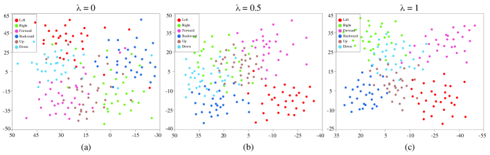
We evaluated model performance by changing the values of , and the results are shown in Table IV. The was introduced to disjoint and by establishing an orthogonal relationship. Performance was improved as the influence of increased according to Table IV. Thus, it demonstrated that orthogonal relationship could improve classification performance. This can also be confirmed through visualization. Fig. 4 provides visualization of features obtained by . When the was not influential ( = 0), the features showed a similar distribution with Fig. 3(b) rather than distinguishing clusters. In Fig 4(b), a clearer clusters were formed, specifically, the features of “left” class are gathered around the cluster. However, numerous features share latent space, especially “Up” class is totally not distinguishable. Finally, features formed clusters by class densely on the center of the cluster in Fig. 4(c). Some features still share the space, but it shows the clearest clusters. Therefore, we confirmed that the enabled the model to extract distinct and decisive features in performance according to results and visualizations. In summary, we demonstrated that the designed modules were trained to obtain two separate latent spaces through the factorization. In addition, jointly training of separate latent spaces derived performance improvement under sparse condition.
V Discussion
V-A Sparse Condition
The goal of this study is to improve classification performance by sufficiently extracting decisive features under sparse condition. Firstly, we considered the definition of sparse condition. The brain region where the EEG signals are generated should be a small area, thus spatial characteristics of the imagery tasks should be similar. Publicly opened MI BCI datasets [34, 62] are mainly composed of imagery tasks that separate brain regions (e.g. foot, tongue, left and right hand) [28, 61]. Jeong et al. [33] proposed single-arm movement imagery tasks such as 6 directions of arm reaching, 3 different grasping. Since all subjects are right-handed, the mainly activated brain region would be the left sensorimotor cortex. Specifically, according to functional brain mapping, meaningful EEG signals are intensively generated only in the middle region of the sensorimotor cortex [63]. To introduce the sparse condition, we selected 6 directions of arm reaching classes because they share the same brain region. Based on provided experimental protocol, we conjecture that it would be fewer distinct temporal and spatial features between classes. Through the experiments, we confirmed that existing methods showed unsatisfactory performance hence conventional feature extraction is not efficient under sparse condition. However further studies are needed to clearly explore sparse condition in various ways because of the lack of ground truth of EEG signals.
V-B Class-common Features
We designed to include unrelated features to the classes. Therefore, it may include common representation of the EEG signals. It is not known whether common information is spatial, temporal, or contains all. In the spatial aspect, features would include information of middle region of the left sensorimotor cortex. On the one hand, in the temporal aspect, features may contain information “reaching arm” over time except for the direction according to the experimental protocol. Ablation study showed that using only was not efficient for classification because it is class-unrelated features as shown in Table III and Fig. 3(a). Nevertheless, it helps the model extract more distinct features when jointly used with . This means that broadens the view of to consider implicit representations in latent space. Indeed acquired features that formed clusters for each class more clearly with the depicted as in Fig. 4.
V-C Class-specific Features
Class-specific features, in this study, are the same as those produced in commonly used training. In Fig. 3(b), the features relatively appear to cluster in the latent space compared to Fig. 3(a) although some features are apparent outliers. In addition, when only was used for classification, the performance was similar to those of existing methods. However, when the classifier considered both and , it acquired the most distinctive representations and showed the highest performance. As a result, we demonstrated that helps acquire more decisive features for classification than under sparse condition.
V-D Orthogonality in EEG Features
The constrains and to be orthogonal to each other. Our approach is that the and are disjoint with each other so that allowing to consider implicit representations in a wider latent space through concatenation. Thus we conjecture that and are different domain features. Thus was introduced to minimize the latent space shared by the two features. As shown in Fig 3(a), , the features from form clusters with numerous outliers in the latent space. As the influence of increases, classification accuracies improved, and features also form clear clusters. Through this, we confirmed that orthogonal constraint allows to use more abundant features from separate latent spaces.
VI Conclusions
In this paper, we defined sparse condition propose a factorization approach that integrates latent space of class-common and class-specific features. Under the sparse condition, existing feature extraction methods face difficulty extracting distinct features, and their performance also decreases. To solve this problem, we introduced a training strategy that factorizes EEG signals in order to obtain distinct features under sparse condition. To this end, we applied a regime of adversarial learning to extract class-common features. The proposed method is trained to deceive the discriminator by extracting features regardless of class. A training strategy is to factorize EEG signals into two types of features so that it allows the classifier to consider the discriminative features from the two different latent spaces. In order to minimize the shared latent spaces by the features, orthogonal constraints were introduced based on the difference loss function. Experimental results demonstrated that the factorization achieved performance improvement in single-arm MI classification accuracy by integrating class-common and class-specific features. Although the proposed method achieved performance improvement, it is necessary to investigate what information class-common features contain and what effect the combination of latent spaces plays in obtaining distinct features. Therefore, our future works are to explore the issues to clearly prove it.
VII Acknowledgements
This work was partly supported by Institute of Information & Communications Technology Planning & Evaluation (IITP) grant funded by the Korea government (MSIT) (No. 2017-0-00432, Development of Non-Invasive Integrated BCI SW Platform to Control Home Appliances and External Devices by User’s Thought via AR/VR Interface; No. 2017-0-00451, Development of BCI based Brain and Cognitive Computing Technology for Recognizing User’s Intentions using Deep Learning; No. 2019-0-00079, Artificial Intelligence Graduate School Program, Korea University).
References
- [1] L. Chen, T. Yang, X. Zhang, W. Zhang, and J. Sun, “Points as queries: Weakly semi-supervised object detection by points,” in Proc. IEEE Comput. Soc. Conf. Comput. Vis. Pattern Recognit. (CVPR), 2021, pp. 8823–8832.
- [2] S.-W. Lee and H.-H. Song, “A new recurrent neural-network architecture for visual pattern recognition,” IEEE trans. Neural Netw., vol. 8, no. 2, pp. 331–340, 1997.
- [3] P. Y. Kao, Y.-J. Lei, C.-H. Chang, C.-S. Chen, M.-S. Lee, and Y.-P. Hung, “Activity recognition using first-person-view cameras based on sparse optical flows,” in Proc. Int. Conf. Pattern Recognit. (ICPR). IEEE, 2021, pp. 81–86.
- [4] D.-G. Lee and S.-W. Lee, “Human interaction recognition framework based on interacting body part attention,” Pattern Recognit., vol. 128, p. 108645, 2022.
- [5] S.-H. Lee, J.-H. Kim, H. Chung, and S.-W. Lee, “Voicemixer: Adversarial Voice Style Mixup,” in Thirty-Fifth Conf. Adv. Neural Inf. Process Syst., Dec, 2021.
- [6] H. Liu, W. Xu, and B. Yang, “Audio-visual speech recognition using a two-step feature fusion strategy,” in Proc. Int. Conf. Pattern Recognit. (ICPR). IEEE, 2021, pp. 1896–1903.
- [7] S.-H. Lee, H.-R. Noh, W.-J. Nam, and S.-W. Lee, “Duration controllable voice conversion via phoneme-based information bottleneck,” IEEE/ACM Trans. Audio, Speech, Language Process., vol. 30, pp. 1173–1183, 2022.
- [8] H. Liu, Y. Wang, and B. Yang, “Mutual alignment between audiovisual features for end-to-end audiovisual speech recognition,” in Proc. Int. Conf. Pattern Recognit. (ICPR). IEEE, 2021, pp. 5348–5353.
- [9] S.-H. Lee, H.-W. Yoon, H.-R. Noh, J.-H. Kim, and S.-W. Lee, “Multi-spectroGAN: High-Diversity and High-Fidelity Spectrogram Generation with Adversarial Style Combination for Speech Synthesis,” in Proc. AAAI Conf. Artif. Intell., vol. 35, no. 14, New York, USA, Feb, 2021, pp. 13 198–13 206.
- [10] J. Devlin, M.-W. Chang, K. Lee, and K. Toutanova, “Bert: Pre-training of deep bidirectional transformers for language understanding,” arXiv preprint arXiv:1810.04805, 2018.
- [11] H. Lee, J. Yoon, B. Hwang, S. Joe, S. Min, and Y. Gwon, “Korealbert: Pretraining a lite bert model for korean language understanding,” in Proc. Int. Conf. Pattern Recognit. (ICPR). IEEE, 2021, pp. 5551–5557.
- [12] Z. Yang, A. Kay, Y. Li, W. Cross, and J. Luo, “Pose-based body language recognition for emotion and psychiatric symptom interpretation,” in Proc. Int. Conf. Pattern Recognit. (ICPR). IEEE, 2021, pp. 294–301.
- [13] M. Lee, L. R. Sanz, A. Barra, A. Wolff, J. O. Nieminen, M. Boly, M. Rosanova, S. Casarotto, O. Bodart, J. Annen et al., “Quantifying arousal and awareness in altered states of consciousness using interpretable deep learning,” Nat. Commun., vol. 13, no. 1, pp. 1–14, 2022.
- [14] J.-H. Cho, J.-H. Jeong, and S.-W. Lee, “Neurograsp: Real-time eeg classification of high-level motor imagery tasks using a dual-stage deep learning framework,” IEEE Trans. Cybern., 2021.
- [15] D.-O. Won, H.-J. Hwang, D.-M. Kim, K.-R. Müller, and S.-W. Lee, “Motion-based rapid serial visual presentation for gaze-independent brain-computer interfaces,” IEEE Trans. Neural Syst. Rehabil. Eng., vol. 26, no. 2, pp. 334–343, 2017.
- [16] K.-T. Kim, H.-I. Suk, and S.-W. Lee, “Commanding a brain-controlled wheelchair using steady-state somatosensory evoked potentials,” IEEE Trans. Neural Syst. Rehabil. Eng., vol. 26, no. 3, pp. 654–665, 2016.
- [17] Y. Chen, A. D. Atnafu, I. Schlattner, W. T. a. Weldtsadik, and S. Fazli, “A high-security EEG-based login system with RSVP stimuli and dry electrodes,” IEEE Trans. Inf. Forensics Secur., vol. 11, no. 12, pp. 2635–2647, 2016.
- [18] H.-I. Suk, S. Fazli, J. Mehnert, K.-R. Müller, and S.-W. Lee, “Predicting bci subject performance using probabilistic spatio-temporal filters,” PloS one, vol. 9, no. 2, p. e87056, 2014.
- [19] D.-Y. Lee, J.-H. Jeong, B.-H. Lee, and S.-W. Lee, “Motor imagery classification using inter-task transfer learning via a channel-wise variational autoencoder-based convolutional neural network,” IEEE Trans. Neural Syst. Rehab. Eng., vol. 30, pp. 226–237, 2022.
- [20] N. J. Hill, D. Gupta, P. Brunner, A. Gunduz, M. A. Adamo, A. Ritaccio, and G. Schalk, “Recording human electrocorticographic (ecog) signals for neuroscientific research and real-time functional cortical mapping,” J. Vis. Exp., no. 64, p. e3993, 2012.
- [21] M.-H. Lee, S. Fazli, J. Mehnert, and S.-W. Lee, “Subject-dependent classification for robust idle state detection using multi-modal neuroimaging and data-fusion techniques in BCI,” Pattern Recognit., vol. 48, no. 8, pp. 2725–2737, 2015.
- [22] L. P. McAvinue and I. H. Robertson, “Measuring motor imagery ability: a review,” Eur. J. Cogn. Psychol., vol. 20, no. 2, pp. 232–251, 2008.
- [23] T. Sousa, C. Amaral, J. Andrade, G. Pires, U. J. Nunes, and M. Castelo-Branco, “Pure visual imagery as a potential approach to achieve three classes of control for implementation of BCI in non-motor disorders,” J. Neural Eng., vol. 14, no. 4, p. 046026, 2017.
- [24] C. S. DaSalla, H. Kambara, M. Sato, and Y. Koike, “Single-trial classification of vowel speech imagery using common spatial patterns,” Neural Netw., vol. 22, no. 9, pp. 1334–1339, Nov. 2009.
- [25] Y. Zhang, H. Zhang, X. Chen, S.-W. Lee, and D. Shen, “Hybrid High-Order Functional Connectivity Networks Using Resting-state Functional MRI for Mild Cognitive Impairment Diagnosis,” Sci. Rep., vol. 7, no. 1, pp. 1–15, 2017.
- [26] B.-H. Lee, J.-H. Jeong, K.-H. Shim, and S.-W. Lee, “Classification of high-dimensional motor imagery tasks based on an end-to-end role assigned convolutional neural network,” in IEEE Int. Conf. Acoust. Speech Signal Process. (ICASSP). IEEE, 2020, pp. 1359–1363.
- [27] N.-S. Kwak, K.-R. Müller, and S.-W. Lee, “A lower limb exoskeleton control system based on steady state visual evoked potentials,” J. Neural. Eng., vol. 12, no. 5, p. 056009, 2015.
- [28] J. Decety, “The neurophysiological basis of motor imagery,” Behav. Brain Res., vol. 77, no. 1-2, pp. 45–52, 1996.
- [29] J.-H. Jeong, N.-S. Kwak, C. Guan, and S.-W. Lee, “Decoding movement-related cortical potentials based on subject-dependent and section-wise spectral filtering,” IEEE Trans. Neural Syst. Rehab. Eng., vol. 28, no. 3, pp. 687–698, 2020.
- [30] B.-H. Kwon, J.-H. Jeong, J.-H. Cho, and S.-W. Lee, “Decoding of Intuitive Visual Motion Imagery Using Convolutional Neural Network under 3D-BCI Training Environment,” in Int. Conf. Sys. Man, and Cybern. (SMC), Toronto, Canada, Oct, 2020, pp. 2966–2971.
- [31] C. S. DaSalla, H. Kambara, M. Sato, and Y. Koike, “Single-trial classification of vowel speech imagery using common spatial patterns,” Neural Netw., vol. 22, no. 9, pp. 1334–1339, 2009.
- [32] C. H. Nguyen, G. K. Karavas, and P. Artemiadis, “Inferring imagined speech using EEG signals: a new approach using Riemannian manifold features,” J. Neural Eng., vol. 15, no. 1, p. 016002, Dec. 2017.
- [33] J.-H. Jeong, J.-H. Cho, K.-H. Shim, B.-H. Kwon, B.-H. Lee, D.-Y. Lee, D.-H. Lee, and S.-W. Lee, “Multimodal signal dataset for 11 intuitive movement tasks from single upper extremity during multiple recording sessions,” GigaScience, vol. 9, no. 10, p. giaa098, Oct. 2020.
- [34] M. Tangermann, K.-R. Müller, A. Aertsen, N. Birbaumer, C. Braun, C. Brunner, R. Leeb, C. Mehring, K. J. Miller, G. Mueller-Putz et al., “Review of the BCI competition IV,” Front. Neurosci., vol. 6, p. 55, 2012.
- [35] D.-Y. Lee, M. Lee, and S.-W. Lee, “Decoding imagined speech based on deep metric learning for intuitive bci communication,” IEEE Trans. Neural Syst. Rehab. Eng., vol. 29, pp. 1363–1374, 2021.
- [36] V. J. Lawhern, A. J. Solon, N. R. Waytowich, S. M. Gordon, C. P. Hung, and B. J. Lance, “EEGNet: a compact convolutional neural network for eeg-based brain–computer interfaces,” J. Neural Eng., vol. 15, no. 5, p. 056013, 2018.
- [37] R. T. Schirrmeister, J. T. Springenberg, L. D. J. Fiederer, M. Glasstetter, K. Eggensperger, M. Tangermann, F. Hutter, W. Burgard, and T. Ball, “Deep learning with convolutional neural networks for EEG decoding and visualization,” Hum. Brain Mapp., vol. 38, no. 11, pp. 5391–5420, 2017.
- [38] A. M. Azab, L. Mihaylova, K. K. Ang, and M. Arvaneh, “Weighted transfer learning for improving motor imagery-based brain–computer interface,” IEEE Trans. Neural Syst. Rehabil. Eng., vol. 27, no. 7, pp. 1352–1359, 2019.
- [39] O.-Y. Kwon, M.-H. Lee, C. Guan, and S.-W. Lee, “Subject-independent brain-computer interfaces based on deep convolutional neural networks,” IEEE Trans. Neural Netw. Learn. Syst., vol. 31, no. 10, pp. 3839–3852, 2020.
- [40] K. Venkatachalam, A. Devipriya, J. Maniraj, M. Sivaram, A. Ambikapathy, and S. A. Iraj, “A novel method of motor imagery classification using EEG signal,” Artif. Intell. Med., vol. 103, p. 101787, 2020.
- [41] J.-H. Jeong, K.-H. Shim, D.-J. Kim, and S.-W. Lee, “Brain-controlled robotic arm system based on multi-directional CNN-BiLSTM network using EEG signals,” IEEE Trans. Neural Syst. Rehabil. Eng., vol. 28, no. 5, pp. 1226–1238, 2020.
- [42] S. U. Amin, M. Alsulaiman, G. Muhammad, M. A. Bencherif, and M. S. Hossain, “Multilevel weighted feature fusion using convolutional neural networks for EEG motor imagery classification,” IEEE Access, vol. 7, pp. 18 940–18 950, 2019.
- [43] N. Lu, T. Li, X. Ren, and H. Miao, “A deep learning scheme for motor imagery classification based on restricted Boltzmann machines,” IEEE Trans. Neural Syst. Rehabil. Eng., vol. 25, no. 6, pp. 566–576, 2016.
- [44] K. K. Ang, Z. Y. Chin, H. Zhang, and C. Guan, “Filter bank common spatial pattern (FBCSP) in brain-computer interface,” in Proc. Int. Jt. Conf. Neural Netw. IEEE, 2008, pp. 2390–2397.
- [45] S. Sakhavi, C. Guan, and S. Yan, “Learning temporal information for brain-computer interface using convolutional neural networks,” IEEE Trans. Neural Netw. Learn. Syst., vol. 29, no. 11, pp. 5619–5629, 2018.
- [46] B. Burle, L. Spieser, C. Roger, L. Casini, T. Hasbroucq, and F. Vidal, “Spatial and temporal resolutions of EEG: Is it really black and white? A scalp current density view,” Int. J. Psychophysiol., vol. 97, no. 3, pp. 210–220, 2015.
- [47] A. A. Torres-García, C. A. Reyes-García, L. Villaseñor-Pineda, and G. García-Aguilar, “Implementing a fuzzy inference system in a multi-objective EEG channel selection model for imagined speech classification,” Expert Syst. Appl., vol. 59, pp. 1–12, Oct. 2016.
- [48] S.-W. Lee and A. Verri, Pattern Recognition with Support Vector Machines: First International Workshop, SVM 2002, Niagara Falls, Canada, August 10, 2002. Proceedings. Springer, 2003, vol. 2388.
- [49] F. Fahimi, S. Dosen, K. K. Ang, N. Mrachacz-Kersting, and C. Guan, “Generative adversarial networks-based data augmentation for brain-computer interface,” IEEE Trans. Neural Netw. Learn. Syst., 2020.
- [50] M.-Y. Liu and O. Tuzel, “Coupled generative adversarial networks,” Adv. Neural Inf. Process. Syst. (NIPS), vol. 29, pp. 469–477, 2016.
- [51] E. Tzeng, J. Hoffman, K. Saenko, and T. Darrell, “Adversarial discriminative domain adaptation,” in Proc. IEEE Comput. Conf. Comput. Vis. Pattern Recognit. (CVPR), 2017, pp. 7167–7176.
- [52] P. Zhong, D. Wang, and C. Miao, “Eeg-based emotion recognition using regularized graph neural networks,” IEEE Trans. Affect. Comput., 2020.
- [53] Y. Li, L. Wang, W. Zheng, Y. Zong, L. Qi, Z. Cui, T. Zhang, and T. Song, “A novel bi-hemispheric discrepancy model for eeg emotion recognition,” IEEE Trans. Cogn. Devel. Syst., vol. 13, no. 2, pp. 354–367, 2020.
- [54] A. Ahmetoğlu and E. Alpaydın, “Hierarchical mixtures of generators for adversarial learning,” in Proc. Int. Conf. Pattern Recognit. (ICPR). IEEE, 2021, pp. 316–323.
- [55] T. Uelwer, A. Oberstra, and S. Harmeling, “Phase retrieval using conditional generative adversarial networks,” in Proc. Int. Conf. Pattern Recognit. (ICPR). IEEE, 2021, pp. 731–738.
- [56] D.-A. Clevert, T. Unterthiner, and S. Hochreiter, “Fast and accurate deep network learning by exponential linear units (elus),” arXiv preprint arXiv:1511.07289, 2015.
- [57] Y. Qi, “Random forest for bioinformatics,” in Ensem. mach. learn., 2012, pp. 307–323.
- [58] K. Bousmalis, G. Trigeorgis, N. Silberman, D. Krishnan, and D. Erhan, “Domain separation networks,” Adv. Neural Inf. Process. Syst., vol. 29, pp. 343–351, 2016.
- [59] M. Salzmann, C. H. Ek, R. Urtasun, and T. Darrell, “Factorized orthogonal latent spaces,” in Proc. Thirteenth Int. Conf. Artif. Intell. Stat. JMLR Workshop and Conference Proceedings, 2010, pp. 701–708.
- [60] I. Loshchilov and F. Hutter, “Decoupled weight decay regularization,” arXiv preprint arXiv:1711.05101, 2017.
- [61] C. M. Michel and D. Brunet, “EEG source imaging: a practical review of the analysis steps,” Front. Neurol., vol. 10, p. 325, 2019.
- [62] P. Ofner, A. Schwarz, J. Pereira, and G. R. Müller-Putz, “Upper limb movements can be decoded from the time-domain of low-frequency eeg,” PloS one, vol. 12, no. 8, p. e0182578, 2017.
- [63] N. E. Crone, D. L. Miglioretti, B. Gordon, and R. P. Lesser, “Functional mapping of human sensorimotor cortex with electrocorticographic spectral analysis. ii. event-related synchronization in the gamma band.” Brain, vol. 121, no. 12, pp. 2301–2315, 1998.