Factored-NeuS: Reconstructing Surfaces, Illumination, and Materials of Possibly Glossy Objects
Abstract.
We develop a method that recovers the surface, materials, and illumination of a scene from its posed multi-view images. In contrast to prior work, it does not require any additional data and can handle glossy objects or bright lighting. It is a progressive inverse rendering approach, which consists of three stages. First, we reconstruct the scene radiance and signed distance function (SDF) with our novel regularization strategy for specular reflections. Our approach considers both the diffuse and specular colors, which allows for handling complex view-dependent lighting effects for surface reconstruction. Second, we distill light visibility and indirect illumination from the learned SDF and radiance field using learnable mapping functions. Third, we design a method for estimating the ratio of incoming direct light represented via Spherical Gaussians reflected in a specular manner and then reconstruct the materials and direct illumination of the scene. Experimental results demonstrate that the proposed method outperforms the current state-of-the-art in recovering surfaces, materials, and lighting without relying on any additional data.
1. Introduction
Reconstructing shape, material, and lighting from multiple views has wide applications in graphics and vision such as virtual reality, augmented reality, and shape analysis. The emergence of neural radiance fields (Mildenhall et al., 2020) provides a framework for high-quality scene reconstruction. Subsequently, many works (Oechsle et al., 2021; Wang et al., 2021; Yariv et al., 2021; Wang et al., 2022; Fu et al., 2022) have incorporated implicit neural surfaces into neural radiance fields, further enhancing the quality of surface reconstruction from multi-views. Recently, several works (Munkberg et al., 2022; Zhang et al., 2021b; Zhang et al., 2021a, 2022b) have utilized coordinate-based networks to predict materials and learned parameters to represent illumination, followed by synthesizing image color using physically-based rendering equations to achieve material and lighting reconstruction. However, these methods typically do not fully consider the interdependence between different components, leading to the following issues with glossy surfaces when using real data.
| Method | Explicit surface extraction | Diffuse/specular color decomposition | Illumination reconstruction | Materials reconstruction | Handles glossy surfaces | No Extra Data? | Code available | Venue |
| NeRV (Srinivasan et al., 2021) | ✗ | ✓ | ✓ | ✓ | ✗ | ✓ | [to appear] | CVPR 2021 |
| PhySG (Zhang et al., 2021a) | ✓ | ✓ | ✓ | ✓ | ✓ | object masks | ✓ | CVPR 2021 |
| NeuS (Wang et al., 2021) | ✓ | ✗ | ✗ | ✗ | ✗ | ✓ | ✓ | NeurIPS 2021 |
| NeRFactor (Zhang et al., 2021b) | ✗ | ✓ | ✓ | ✓ | ✗ | BRDF dataset | ✓ | SG Asia 2021 |
| Ref-NeRF (Verbin et al., 2022) | ✗ | ✓ | ✗ | ✗ | ✓ | ✓ | ✓ | CVPR 2022 |
| NVDiffrec (Munkberg et al., 2022) | ✓ | ✓ | ✓ | ✓ | ✗ | object masks | ✓ | CVPR 2022 |
| IndiSG (Zhang et al., 2022b) | ✓ | ✓ | ✓ | ✓ | ✗ | object masks | ✓ | CVPR 2022 |
| Geo-NeuS (Fu et al., 2022) | ✓ | ✗ | ✗ | ✗ | ✗ | point clouds | ✓ | NeurIPS 2022 |
| BakedSDF (Yariv et al., 2023) | ✓ | ✓ | ✗ | ✗ | ✗ | ✓ | ✗ | SG 2023 |
| TensoIR (Jin et al., 2023) | ✗ | ✓ | ✓ | ✓ | ✗ | ✓ | ✓ | CVPR 2023 |
| NeFII (Wu et al., 2023a) | ✓ | ✓ | ✓ | ✓ | ✗ | ✓ | ✗ | CVPR 2023 |
| Ref-NeuS (Ge et al., 2023) | ✓ | ✗ | ✗ | ✗ | ✓ | ✓ | [to appear] | arXiv 2023/03 |
| Surf (Wu et al., 2023b) | ✓ | ✗ | ✗ | ✗ | ✗ | object masks | [to appear] | arXiv 2023/03 |
| NeILF++ (Zhang et al., 2023b) | ✓ | ✓ | ✓ | ✓ | ✗ | ✓ | [to appear] | arXiv 2023/03 |
| ENVIDR (Liang et al., 2023) | ✓ | ✓ | ✓ | ✓ | ✓ | BRDF dataset | [to appear] | arXiv 2023/03 |
| NeMF (Zhang et al., 2023a) | ✗ | ✓ | ✓ | ✓ | ✗ | ✓ | ✗ | arXiv 2023/04 |
| NeAI (Zhuang et al., 2023) | ✗ | ✓ | ✓ | ✓ | ✓ | ✓ | [to appear] | arXiv 2023/04 |
| Factored-NeuS(ours) | ✓ | ✓ | ✓ | ✓ | ✓ | ✓ | [to appear] | - |
First, surfaces with glossy materials typically result in highlights. The best current methods for reconstructing implicit neural surfaces rarely consider material information and directly reconstruct surfaces. The surface parameters can then be frozen for subsequent material reconstruction. Since neural radiance fields typically model such inconsistent colors as bumpy surface as shown in Fig. 1, the artifacts from surface reconstruction will affect material reconstruction if surfaces and materials are reconstructed sequentially. Second, a glossy surface can affect the decomposition of the reflected radiance into a diffuse component and a specular component. Typically, the specular component leaks into the diffuse component, resulting in inaccurate modeling as shown in Fig. 2. Third, focusing on synthetic data makes it easier to incorporate complex physically-based rendering algorithms, but they may not be robust enough to work on real data.
In this work, we consider the impact of glossy surfaces on surface and material reconstruction. To consider glossy surfaces represented by signed distance functions (SDFs), our method not only synthesizes views with highlights but also decomposes the highlight views into diffuse and specular reflection components. This approach compensates for the modeling capability of anisotropic radiance in rendering and produces correct results for glossy surface reconstruction. In order to better recover diffuse and specular components, we estimate a parameter to represent the ratio of incoming light reflected in a specular manner. By introducing this parameter into a Spherical Gaussian representation of the BRDF, we can better model the reflection of glossy surfaces and decompose more accurate diffuse albedo information. Furthermore, we propose predicting continuous light visibility for signed distance functions to further enhance the quality of reconstructed materials and illumination. Our experimental results have shown that our factorization of surface, materials, and illumination achieves state-of-the-art performance on both synthetic and real datasets. Our main contribution is that we improve surface, material, and lighting reconstruction compared to PhySG (Zhang et al., 2021a), NVDiffRec (Munkberg et al., 2022), and IndiSG (Zhang et al., 2022b), the leading published competitors.
We believe that the good results of our approach compared to much recently published and unpublished work in material reconstruction is that we primarily developed our method on real data. The fundamental challenge for working on material and lighting reconstruction is the lack of available ground truth information for real datasets. Our solution to this problem was to work with real data and try to improve surface reconstruction as our main metric by experimenting with different materials and lighting decompositions as a regularizer. While we could not really measure the success of the material and lighting reconstruction directly, we could indirectly observe improvements in the surface metrics. By contrast, most recent and concurrent work uses surface reconstruction and real data more as an afterthought. This alternative route is to first focus on developing increasingly complex material and lighting reconstruction on synthetic data. However, we believe that this typically does not translate as well to real data as our approach.
2. Related work
Neural radiance fields. NeRF (Mildenhall et al., 2020) is a seminal work in 3D reconstruction. It utilizes MLPs to predict view-dependent radiance and density in 3D space and renders an object or scene using volume rendering. Important improvements were proposed by Mip-NeRF (Barron et al., 2021) and Mip-NeRF360 (Barron et al., 2022). Another noteworthy line of work explores the combination of different data structures with MLPs, such as factored volumes (Chan et al., 2022; Chen et al., 2022; Wang et al., 2023) or voxels (Müller et al., 2022; Reiser et al., 2021; Yu et al., 2021).
There are multiple approaches to extend neural radiance fields to reconstruct material information. To model specular reflections, NeRFReN (Guo et al., 2022) uses another MLP to predict the reflection properties. Ref-NeRF (Verbin et al., 2022), on the other hand, uses a reflection vector as an input for learning the specular component of radiance. Recently, Ref-NeuS (Ge et al., 2023) also models the radiance field using the reflection direction and proposes a reflection-aware photometric loss to reconstruct reflective surfaces. BakeSDF (Yariv et al., 2023) achieves good results in decomposing diffuse color and specular reflection components by baking view-dependent and view-independent appearance into the vertices of triangle meshes. These methods did not explicitly model the lighting environment, so the result is not a proper material model.
Implicit neural surfaces. Implicit neural surfaces are typically represented by occupancy functions or signed distance fields (SDFs). Some early works (Chen and Zhang, 2019; Mescheder et al., 2019; Park et al., 2019) take point clouds as input and output implicit neural surface representations. Subsequently, many works have studied how to obtain implicit neural surfaces from images. DVR (Niemeyer et al., 2020) and IDR (Yariv et al., 2020) render images by calculating the appearance information of the intersection points between rays and surfaces. However, this type of rendering has a drawback for surface reconstruction using gradient descent as information is only considered on the surface. Subsequent work therefore calculates the appearance information of all sampling points on the ray and obtains the rendered pixel through weighting strategies along the ray. Examples are UNISURF (Oechsle et al., 2021), VolSDF (Yariv et al., 2021), NeuS (Wang et al., 2021), HF-NeuS (Wang et al., 2022), and Geo-NeuS (Fu et al., 2022). By using gradients in the entire space, these methods are able to obtain higher-quality implicit neural surfaces.
Joint reconstruction of surface, material, and illumination. Ideally, we would like to jointly reconstruct the 3D geometry, material properties, and lighting conditions of a scene from 2D images. This is a very challenging and ill-posed problem, but several recent papers have made progress in this direction. PhySG (Zhang et al., 2021a), NeRFactor (Zhang et al., 2021b), and NeROIC (Kuang et al., 2022) use Spherical Gaussians, point light sources, and spherical harmonics, respectively, to decompose unknown lighting from a set of images. NeRV (Srinivasan et al., 2021) considers indirect illumination but requires known environment lighting. NeRD (Boss et al., 2021a) later extends this to handle input images with different lighting conditions. Using an illumination integration network, Neural-PIL (Boss et al., 2021b) further reduces the computational cost of lighting integration. IRON (Zhang et al., 2022a) uses SDF-based volume rendering methods to obtain better geometric details in the shape recovery stage. NVDiffrec (Munkberg et al., 2022) explicitly extracts triangle mesh from tetrahedral representation for better material and lighting modeling. IndiSG (Zhang et al., 2022b) uses Spherical Gaussians to represent indirect illumination and achieves good lighting decomposition results. Some concurrent works (Jin et al., 2023; Wu et al., 2023a; Zhang et al., 2023b, a) continue to improve the efficiency and quality of inverse rendering, but lack to consider cases with a glossy appearance. NeAI (Zhuang et al., 2023) proposes neural ambient illumination to enhance the rendering quality of glossy appearance. While ENVIDR (Liang et al., 2023) can obtain material and environmental lighting information for glossy surfaces, the proposed neural renderer requires pre-training on a new dataset with gt SDF values and cannot explicitly model light visibility. Despite a lot of recent activity in this area, existing frameworks still struggle to effectively reconstruct reflective or glossy surfaces, lighting, and material information directly from images, especially real-world captured images. Tab. 1 provides a comprehensive overview of the capabilities of the recent inverse rendering techniques.
3. Method
3.1. Overview
Our framework has three training stages to gradually decompose the shape, materials, and illumination. The input to our framework is a set of images. In the first stage, we reconstruct the surface from a (possibly glossy) appearance decomposing the color into diffuse and specular components. After that, we use the reconstructed radiance field to extract direct illumination visibility and indirect illumination in the second stage. Having them decomposed from the radiance field allows for the recovery of the direct illumination map and materials’ bidirectional reflectance distribution function (BRDF), which we perform in the final stage.
3.2. Preliminaries
Volume rendering. The radiance of the pixel corresponding to a given ray at the origin towards direction is calculated using the volume rendering equation, which involves an integral along the ray with boundaries and ( and are parameters to define the near and far clipping plane). This calculation requires the knowledge of the volume density and directional color for each point within the volume.
| (1) |
The volume density is used to calculate the accumulated transmittance :
| (2) |
It is then used to compute a weighting function to weigh the sampled colors along the ray to integrate into radiance .
Surface rendering. The radiance reflected from a surface point in direction is an integral of bidirectional reflectance distribution function (BRDF) and illumination over half sphere , centered at normal of the surface point :
| (3) |
where is the illumination on from the incoming light direction , and is BRDF, which is the proportion of light reflected from direction towards direction at the point .
3.3. Stage 1: Surface reconstruction from glossy appearance
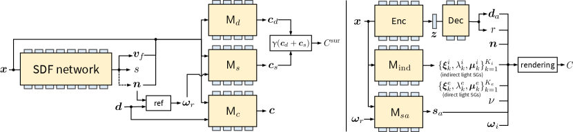
Current inverse rendering methods first recover implicit neural surfaces, typically represented as SDFs, from multi-view images to recover shape information, then freeze the parameters of neural surfaces to further recover the material. However, this approach does not consider specular reflections that produce highlights and often models this inconsistent color as bumpy surface geometry as depicted in Fig. 1. This incorrect surface reconstruction has a negative impact on subsequent material reconstruction. We propose a neural surface reconstruction method that considers the appearance, diffuse color, and specular color of glossy surfaces at the same time, whose architecture is given in Fig. 3. Our inspiration comes from the following observations. First, according to Geo-NeuS, using SDF point cloud supervision can make the colors of surface points and volume rendering more similar. We abandoned the idea of using additional surface points to supervise SDFs and directly use two different MLPs to predict the surface rendering and volume rendering results, and narrow the gap between these two colors using network training. In addition, when modeling glossy surfaces, Ref-NeRF proposes a method of decomposing appearance into diffuse and specular components, which can better model the glossy appearance. We propose to simultaneously optimize the volume appearance, surface diffuse radiance, and specular radiance of surface points, which can achieve an improved surface reconstruction of glossy surfaces.
Shape representation. We model shape as a signed distance function , which maps a 3D point to its signed distance value and a feature vector . SDF allows computing a normal directly by calculating the gradient: .
Synthesize appearance. Learning implicit neural surfaces from multi-view images often requires synthesizing appearance to optimize the underlying surface. The recent use of volume rendering in NeuS (Wang et al., 2021) has been shown to better reconstruct surfaces. According to Eq. 1, the discretization formula for volume rendering is as follows with sampled points on the ray.
| (4) |
where , which is discrete opacity values following NeuS where is a sigmoid function and is the discrete transparency. Similar to the continuous case, we can also define discrete weights .
To compute color on the point , we define a color mapping from any 3D point given its feature vector , normal and ray direction .
Synthesize diffuse and specular components. In addition to synthesizing appearance, we also synthesize diffuse and specular components. This idea comes from surface rendering, which is better at simulating the reflection of light on a surface. From Eq. 3, the radiance of surface point and outgoing viewing direction can be decomposed into two parts: diffuse and specular radiances.
| (5) | ||||
| (6) | ||||
| (7) |
We define two neural networks to predict diffuse and specular components separately. Diffuse radiance refers to the scattered and spread-out light that illuminates a surface or space evenly and without distinct shadows or reflections. We define a mapping for diffuse radiance that maps surface points , surface normals , and feature vectors to diffuse radiance. For simplicity, we assume that the diffuse radiance is not related to the outgoing viewing direction .
Specular radiance is usually highly dependent on the viewing direction. Ref-NeRF (Verbin et al., 2022) proposes to use the reflection direction instead of the viewing direction to model the glossy appearance in a compact way. However, from Eq. 7, we can observe that specular radiance is also highly dependent on the surface normal, which is particularly important when reconstructing SDF. In contrast to Ref-NeRF, we further condition specular radiance on the surface normal. Therefore, we define specular radiance , which maps surface points , outgoing viewing direction , surface normals , and feature vectors to specular radiance, where .
Surface rendering focuses the rendering process on the surface, allowing for a better understanding of highlights on the surface compared to volume rendering, but requires calculating surface points. We sample points on the ray . We query the sampled points to find the first point whose SDF value is less than zero . Then the point sampled before has the SDF value greater than or equal to zero . To account for the possibility of rays interacting with objects and having multiple intersection points, we select the first point with a negative SDF value to solve this issue.
We use two neural networks to predict the diffuse radiance and specular radiance of two sampling points and . The diffuse radiance of the two points calculated by the diffuse network will be and . The specular radiance of the two points calculated by the specular network will be and . Therefore, the diffuse radiance and specular radiance of the surface point can be calculated as follows.
| (8) | ||||
| (9) |
The final radiance of the intersection of the ray and the surface is calculated by a tone mapping as follows.
| (10) |
where is a pre-defined tone mapping function that converts linear color to sRGB (Verbin et al., 2022) while ensuring that the resulting color values are within the valid range of [0, 1] by clipping them accordingly.
Training strategies. In our training process, we define three loss functions, namely volume radiance loss , surface radiance loss , and regularization loss . The volume radiance loss is measured by calculating the distance between the ground truth colors and the volume radiances of a subset of rays , which is defined as follows.
| (11) |
The surface radiance loss is measured by calculating the distance between the ground truth colors and the surface radiances . During the training process, only a few rays have intersection points with the surface. We only care about the set of selected rays , which satisfies the condition that each ray exists point whose SDF value is less than zero and not the first sampled point. The loss is defined as follows.
| (12) |
is an Eikonal loss term on the sampled points. Eikonal loss is a regularization loss applied to a set of sampling points , which is used to constrain the noise in signed distance function (SDF) generation.
| (13) |
We use weights and to balance the impact of these three losses. The overall training weights are as follows.
| (14) |
3.4. Stage 2: Learning a direct lighting visibility and indirect illumination
At this stage, we focus on predicting the lighting visibility and indirect illumination of a surface point under different incoming light direction using the SDF in the first stage. Therefore, we need first to calculate the position of the surface point . In stage one, we have calculated two sampling points near the surface. As Geo-NeuS (Fu et al., 2022), we weigh these two sampling points to obtain a surface point as follows.
| (15) |
Learning lighting visibility. Visibility is an important factor in shadow computation. It calculates the visibility of the current surface point in the direction of the incoming light . Path tracing of the SDF is commonly used to obtain a binary visibility (0 or 1) as used in IndiSG (Zhang et al., 2022b), but this kind of visibility is not friendly to network learning. Inspired by NeRFactor (Zhang et al., 2021b), we propose to use an integral representation with the continuous weight function (from 0 to 1) for the SDF to express light visibility. Specifically, we establish a neural network , that maps the surface point and incoming light direction to visibility, and the ground truth value of light visibility is obtained by integrating the weights of the SDF of sampling points as in Eq. 4 along the incoming light direction and can be expressed as follows.
| (16) |
The weights of the light visibility network are optimized by minimizing the loss between the calculated ground truth values and the predicted values of a set of sampled incoming light directions . This pre-integrated technique can reduce the computational burden caused by the integration for subsequent training.
| (17) |
| DTU 63 | DTU 97 | DTU 110 | DTU 122 | Mean | Pot | Funnel | Snowman | Jug | Mean | |
| NeuS (Wang et al., 2021) | 1.01 | 1.21 | 1.14 | 0.54 | 0.98 | 2.09 | 3.93 | 1.40 | 1.81 | 2.31 |
| Geo-NeuS (Fu et al., 2022) | 0.96 | 0.91 | 0.70 | 0.37 | 0.73 | 1.88 | 2.03 | 1.64 | 1.68 | 1.81 |
| PhySG (Zhang et al., 2021a) | 4.16 | 4.99 | 3.57 | 1.42 | 3.53 | 14.40 | 7.39 | 1.55 | 7.59 | 7.73 |
| IndiSG (Zhang et al., 2022b) | 1.15 | 2.07 | 2.60 | 0.61 | 1.61 | 5.62 | 4.05 | 1.74 | 2.35 | 3.44 |
| Factored-NeuS (ours) | 0.99 | 1.15 | 0.89 | 0.46 | 0.87 | 1.54 | 1.95 | 1.31 | 1.40 | 1.55 |
Learning indirect illumination. Indirect illumination refers to the light that is reflected or emitted from surfaces in a scene and then illuminates other surfaces, rather than directly coming from a light source, which contributes to the realism of rendered images. Following IndiSG (Zhang et al., 2022b), we parameterize indirect illumination via Spherical Gaussians (SGs) as follows.
| (18) |
where , , and are the lobe axis, sharpness, and amplitude of the -th Spherical Gaussian, respectively. For this, we train a network that maps the surface point to the parameters of indirect light SGs. Similar to learning visibility, we randomly sample several directions from the surface point to obtain (pseudo) ground truth . Some of these rays have intersections with other surfaces, thus, is the direction pointing from to . We query our proposed color network to get the (pseudo) ground truth indirect radiance as follows.
| (19) |
where is the normal on the point . We also use loss to train the network.
| (20) |
3.5. Stage 3: Recovering materials and direct illuminations
Reconstructing good materials and lighting from scenes with highlights is a challenging task. Following prior works (Zhang et al., 2022b, 2021a), we use the Disney BRDF model (Burley and Studios, 2012) and represent BRDF via Spherical Gaussians (Zhang et al., 2021a). Direct (environment) illumination is represented using SGs:
| (21) |
and render diffuse radiance and specular radiance of direct illumination in a way similar to Eq. 6.
| (22) | ||||
| (23) |
where is diffuse albedo.
To reconstruct a more accurate specular reflection effect, we use an additional neural network to predict the specular albedo. The modified BRDF is as follows:
| (24) |
For indirect illumination, the radiance is extracted directly from another surface and does not consider light visibility. The diffuse radiance and specular radiance of indirect illumination are as follows
| (25) |
| (26) |
Our final synthesized appearance is and can be supervised by the following RGB loss.
| (27) |
3.6. Implementation details
Our full model is composed of several MLP networks, each one of them having a width of 256 hidden units unless otherwise stated. In Stage 1, the SDF network is composed of 8 layers and includes a skip connection at the 4-th layer, similar to NeuS (Wang et al., 2021). The input 3D coordinate is encoded using positional encoding with 6 frequency scales. The diffuse color network utilizes a 4-layer MLP, while the input surface normal is positional-encoded using 4 scales. For the specular color network , a 4-layer MLP is employed, and the reflection direction is also positional-encoded using 4 frequency scales.
In Stage 2, the light visibility network has 4 layers. To better encode the input 3D coordinate , positional encoding with 10 frequency scales is utilized. The input view direction is also positional-encoded using 4 scales. The indirect light network in stage 2 comprises 4 layers.
In stage 3, the encoder part of the BRDF network consists of 4 layers, and the input 3D coordinate is positional-encoded using 10 scales. The output latent vector has 32 dimensions, and we impose a sparsity constraint on the latent code , following IndiSG (Zhang et al., 2022b). The decoder part of the BRDF network is a 2-layer MLP with a width of 128, and the output has 4 dimensions, including the diffuse albedo and roughness . Finally, the specular albedo network uses a 4-layer MLP, where the input 3D coordinate is positional-encoded using 10 scales, and the input reflection direction is positional-encoded using 4 scales.
The learning rate for all three stages begins with a linear warm-up from 0 to during the first 5K iterations. It is controlled by the cosine decay schedule until it reaches the minimum learning rate of , which is similar to NeuS. The weights for the surface color loss are set for 0.1, 0.6, 0.6, and 0.01 for DTU, SK3D, Shiny, and the IndiSG dataset, respectively. We train our model for 300K iterations in the first stage, which takes 11 hours in total. For the second and third stages, we train for 40K iterations, taking around 1 hour each. The training was performed on a single NVIDIA RTX 4090 GPU.
| Baloons | Hotdog | Chair | Jugs | Mean | |||||||||||
| albedo | illumination | rendering | albedo | illumination | rendering | albedo | illumination | rendering | albedo | illumination | rendering | albedo | illumination | rendering | |
| PhySG | 15.91 | 13.89 | 27.83 | 13.95 | 11.69 | 25.13 | 14.86 | 12.26 | 28.32 | 16.84 | 10.92 | 28.20 | 15.39 | 12.19 | 27.37 |
| NVDiffrec | 26.88 | 14.63 | 29.90 | 13.60 | 22.43 | 33.68 | 21.12 | 15.56 | 29.16 | 11.20 | 10.47 | 25.30 | 20.41 | 13.56 | 29.51 |
| IndiSG | 21.95 | 25.24 | 24.40 | 26.43 | 21.87 | 31.77 | 24.71 | 22.17 | 24.98 | 21.44 | 20.59 | 24.91 | 23.63 | 22.47 | 26.51 |
| Ours w/o SAI | 24.09 | 25.97 | 28.82 | 30.58 | 23.50 | 36.05 | 25.23 | 22.13 | 32.64 | 19.64 | 20.40 | 33.56 | 24.89 | 23.00 | 32.77 |
| Ours | 25.79 | 21.79 | 33.89 | 30.72 | 20.23 | 36.71 | 26.33 | 20.97 | 34.58 | 22.94 | 21.84 | 36.48 | 26.28 | 21.21 | 35.41 |
4. Experiments
4.1. Evaluation setup
Datasets. To evaluate the quality of surface reconstruction, we use the DTU (Jensen et al., 2014), SK3D (Voynov et al., 2022), and Shiny (Verbin et al., 2022) datasets. DTU and SK3D are two real-world captured datasets, while Shiny is synthetic. In DTU, each scene is captured by 49 or 64 views of 16001200 resolution. From this dataset, we select 3 scenes with specularities to verify our proposed method in terms of surface quality and material decomposition. In the SK3D dataset, the image resolution is 23681952, and 100 views are provided for each scene. This dataset contains more reflective objects with complex view-dependent lighting effects that pose difficulties in surface and material reconstruction. From SK3D, we select 4 glossy surface scenes with high levels of glare to validate our proposed method. The Shiny dataset has 5 different glossy objects rendered in Blender under conditions similar to NeRF’s dataset (100 training and 200 testing images per scene). The resolution of each image is 800800.
To evaluate the effectiveness of material and lighting reconstruction, we use the dataset provided by IndiSG (Zhang et al., 2022b), which has self-occlusion and complex materials. Each scene has 100 training images of 800 800 resolution. To evaluate the quality of material decomposition, the dataset also provides diffuse albedo, roughness, and masks for testing.
Baselines. Our main competitors are the methods that can also reconstruct all three scene properties: surface geometry, materials, and illumination. We choose NVDiffRec (Munkberg et al., 2022), PhySG (Zhang et al., 2021a), and IndiSG (Zhang et al., 2022b) due to their popularity and availability of the source code. NVDiffRec uses tetrahedral marching to extract triangle meshes and obtains good material decomposition using a triangle-based renderer. PhySG optimizes geometry and material information at the same time using a Spherical Gaussian representation for direct lighting and material. IndiSG first optimizes geometry and then uses a Spherical Gaussian representation for indirect lighting to improve the quality of material reconstruction.
Apart from that, we also compare against more specialized methods for individual quantitative and qualitative comparisons to provide additional context for our results. For surface reconstruction quality, we compare our method to NeuS (Wang et al., 2021) and Geo-NeuS (Fu et al., 2022). NeuS is a popular implicit surface reconstruction method that achieves strong results without reliance on extra data. Geo-NeuS improves upon NeuS by using additional point cloud supervision, obtained from structure from motion (SfM) (Schönberger and Frahm, 2016). We also show a qualitative comparison to Ref-NeRF (Verbin et al., 2022), which considers material decomposition, but due to modeling geometry using density function, it has difficulty extracting smooth geometry.
Evaluation metrics. We use the official evaluation protocol to compute the Chamfer distance (lower values are better) for the DTU dataset and also use the Chamfer distance for the SK3D dataset. We utilize the PSNR metric (higher values are better), to quantitatively evaluate the quality of rendering, material, and illumination. We follow IndiSG (Zhang et al., 2022b) and employ masks to compute the PSNR metric in the foreground to evaluate the quality of materials and rendering.
4.2. Surface reconstruction quality
We first demonstrate quantitative results in terms of Chamfer distance. IndiSG and PhySG share the same surface reconstruction method, but PhySG optimizes it together with the materials, while IndiSG freezes the underlying SDF after its initial optimization. We list the numerical results for IndiSG and PhySG for comparison. NVDiffrec is not as good for surface reconstruction as we verify qualitatively in Fig. 5. For completeness, we also compare our method against NeuS and Geo-NeuS. First, we list quantitative results on the DTU dataset and SK3D dataset in Tab. 2. It should be noted that NeuS and Geo-NeuS can only reconstruct surfaces from multi-views, while our method and IndiSG can simultaneously tackle shape, material, and lighting. As shown in the table, Geo-NeuS achieves better performance on the DTU dataset because the additional sparse 3D points generated by structure from motion (SfM) for supervising the SDF network are accurate. However, on the SK3D scenes with glossy surfaces, these sparse 3D points cannot be generated accurately by SFM, leading to poor surface reconstruction by Geo-NeuS. In contrast, our approach can reconstruct glossy surfaces on both DTU and SK3D without any explicit geometry information. Compared with IndiSG, PhySG cannot optimize geometry and material information well simultaneously on real-world acquired datasets with complex lighting and materials. Our method is the overall best method on SK3D. Most importantly, we demonstrate large improvements over IndiSG and PhySG, our main competitors, on both DTU and SK3D.
We further demonstrate the qualitative experimental comparison results in Fig. 4. It can be seen that although Geo-NeuS has the best quantitative evaluation metrics, it loses some of the fine details, such as the small dents on the metal can in DTU 97. By visualizing the results of the SK3D dataset, we can validate that our method can reconstruct glossy surfaces without explicit geometric supervision.
We then show the qualitative results for surface reconstruction compared with NeuS, Ref-NeRF, IndiSG, PhySG, and NVDiffrec on the Shiny dataset, which is a synthetic dataset with glossy surfaces. From Fig. 5, we can observe that NeuS is easily affected by highlights, and the geometry reconstructed by Ref-NeRF has strong noise. PhySG is slightly better than IndiSG on the Shiny synthetic dataset with jointly optimizing materials and surfaces, such as toaster and car scenes, but still can not handle complex highlights. NVDiffrec works well on the teapot model but fails on other more challenging glossy surfaces. Our method is able to produce clean glossy surfaces without being affected by the issues caused by highlights. Overall, our approach demonstrates superior performance in surface reconstruction, especially on glossy surfaces with specular highlights.
4.3. Material reconstruction and rendering quality
In Tab. 3, we evaluate the quantitative results in terms of PSNR metric for material and illumination reconstruction on the IndiSG dataset compared with PhySG, NVDiffrec, and IndiSG. For completeness, we also compare to the case where the specular albedo improvement was not used in Stage 3 (See in Eq. 24 in Section 3.5). Regarding diffuse albedo, although NVDiffrec showed a slight improvement over us in the balloons scene, we achieved a significant improvement over NVDiffrec in the other three scenes. Our method achieved the best results in material reconstruction. Moreover, our method achieves the best results in illumination quality without using the specular albedo improvement. Additionally, our method significantly outperforms other methods in terms of rendering quality and achieves better appearance synthesis results. We present the qualitative results of material reconstruction in Fig. 6, which shows that our method has better detail capture compared to IndiSG and PhySG, such as the text on the balloon. Although NVDiffrec can reconstruct the nails on the backrest, its material decomposition effect is not realistic. The materials reconstructed by our method are closer to ground truth ones. We also demonstrate the material decomposition effectiveness of our method on Shiny datasets with glossy surfaces, as shown in Fig. 7. We showcase the diffuse albedo and rendering results of NVDiffrec, IndiSG, and our method. The rendering results indicate that our method can restore the original appearance with specular highlights more accurately, such as the reflections on the helmet and toaster compared to the IndiSG and NVDiffrec methods. The material reconstruction results show that our diffuse albedo contains less specular reflection information compared to other methods, indicating our method has better ability to suppress decomposition ambiguity caused by specular highlights.
| Method | Alb | Rough | Rend | Illu |
| IndiSG (Zhang et al., 2022b) | 26.44 | 15.97 | 31.78 | 21.88 |
| Ours w/o SAI w/o VI w/o SI | 29.31 | 16.98 | 35.48 | 23.48 |
| Ours w/o SAI w/o VI | 29.64 | 17.86 | 36.36 | 23.41 |
| Ours w/o SAI | 30.58 | 18.83 | 36.05 | 23.50 |
| Ours | 30.76 | 23.10 | 36.71 | 20.24 |
In addition to the synthetic datasets with ground truth decomposed materials, we also provide qualitative results on real-world captured datasets such as DTU and SK3D in Fig. 8. From the DTU data, we can observe that our method has the ability to separate the specular reflection component from the diffuse reflection component, as seen in the highlights on the apple, can, and golden rabbit. Even when faced with a higher intensity of specular reflection, as demonstrated in the example showcased in SK3D, our method excels at preserving the original color in the diffuse part and accurately separating highlights into the specular part.
| NeuS | 1Vol + 1Sur | 1Vol + 2Vol | Ours (full) |
| 2.09 | 2.01 | 1.91 | 1.88 |
4.4. Ablation study
Materials and illumination. We conduct an ablation study on the different components we proposed by evaluating their material and lighting performance on a complex scene, the hotdog, as shown in Tab. 4. “SI” refers to surface improvement, which means using networks to synthesize diffuse and specular color at the same time. “VI” stands for visibility improvement, which involves a continuous light visibility supervision based on the SDF. and “SAI” refers to specular albedo improvement, which incorporates specular albedo into the BRDF of Spherical Gaussians. We compare different settings in terms of diffuse albedo, roughness, appearance synthesis, and illumination. We used IndiSG as a reference and find that introducing volume rendering can improve the accuracy of material and lighting reconstruction. When the surface has no defects, further performing the surface improvement will enhance the quality of roughness and rendering but may cause a decrease in lighting reconstruction quality. Making the visibility supervision continuous improves the reconstruction of diffuse albedo, roughness, and lighting, but it also affects rendering quality. Introducing specular albedo can greatly improve roughness and rendering quality but negatively affect lighting reconstruction quality. We further show qualitative results in Fig. 10. It can be observed that after improving the light visibility, the white artifacts at the edges of the plate in diffuse albedo are significantly reduced. Introducing specular albedo also makes the sausage appear smoother and closer to its true color roughness, represented by black. In terms of lighting, when not using specular albedo, the lighting reconstruction achieves the best result, indicating a clearer reconstruction of ambient illumination. In summary, our ablation study highlights the importance of taking into account various factors when reconstructing materials and illumination from images. By evaluating the performance of different modules, we can better understand their role in improving the reconstruction quality.
Surface reconstruction. To validate our surface reconstruction strategy in Stage 1, we selected the Pot scene from SK3D and ablated the method the following way. “1Vol + 1Sur” means that we only use volume rendering and surface rendering MLPs for surface reconstruction, without decomposing material information into diffuse and specular components. “1Vol + 2Vol” means we use two volume reconstructions where one of them is split into diffuse and specular components. Just using “2Vol” to split diffuse and specular components will fail to reconstruct the correct surface due to inaccurate normal vectors in reflection direction computation, especially when modeling objects with complex materials or lighting effects. We provide the quantitative (Chamfer distance) and qualitative results of different frameworks in Tab. 5 and Fig. 9, respectively. It can be seen that synchronizing the volume color and the color on the surface point has a certain effect in suppressing concavities, but still cannot meet the requirements for complex glossy surfaces with strong reflections. Using volume rendering to decompose diffuse and specular components can result in excessive influence from non-surface points, which still causes small concavities. When combining these two methods, our approach can achieve reconstruction results without concavities.
5. Conclusions
In this work, we propose Factored-NeuS, a novel approach to inverse rendering that reconstructs geometry, material, and lighting from multiple views. Our first contribution is to simultaneously synthesize the appearance, diffuse radiance, and specular radiance during surface reconstruction, which allows the geometry to be unaffected by glossy highlights. Our second contribution is to train networks to estimate reflectance albedo and learn a visibility function supervised by continuous values based on the SDF, so that our method is capable of better decomposing material and lighting. Experimental results show that our method surpasses the state-of-the-art in both geometry reconstruction quality and material reconstruction quality. A future research direction is how to effectively decompose materials for fine structures, such as nails on a backrest of a chair.
In certain scenarios, our method still faces difficulties. For mesh reconstruction, we can only enhance results on scenes with smooth surfaces and few geometric features. Despite improvements on the glossy parts in the DTU 97 results, the overall Chamfer distance does not significantly decrease. As seen in Fig. 6, the reconstructed albedo of the chair still lacks some detail. The nails on the chair and the textures on the pillow are not accurately captured in the reconstructed geometry. Moreover, we do not foresee any negative societal implications directly linked to our research on surface reconstruction.
In future work, we would like to work on the reconstruction of dynamic objects and humans. We also would like to include additional data acquisition modalities for improved reconstruction.
References
- (1)
- Barron et al. (2021) Jonathan T Barron, Ben Mildenhall, Matthew Tancik, Peter Hedman, Ricardo Martin-Brualla, and Pratul P Srinivasan. 2021. Mip-nerf: A multiscale representation for anti-aliasing neural radiance fields. In Proceedings of the IEEE/CVF International Conference on Computer Vision. 5855–5864.
- Barron et al. (2022) Jonathan T Barron, Ben Mildenhall, Dor Verbin, Pratul P Srinivasan, and Peter Hedman. 2022. Mip-nerf 360: Unbounded anti-aliased neural radiance fields. In Proceedings of the IEEE/CVF Conference on Computer Vision and Pattern Recognition. 5470–5479.
- Boss et al. (2021a) Mark Boss, Raphael Braun, Varun Jampani, Jonathan T Barron, Ce Liu, and Hendrik Lensch. 2021a. Nerd: Neural reflectance decomposition from image collections. In Proceedings of the IEEE/CVF International Conference on Computer Vision. 12684–12694.
- Boss et al. (2021b) Mark Boss, Varun Jampani, Raphael Braun, Ce Liu, Jonathan Barron, and Hendrik Lensch. 2021b. Neural-pil: Neural pre-integrated lighting for reflectance decomposition. Advances in Neural Information Processing Systems 34 (2021), 10691–10704.
- Burley and Studios (2012) Brent Burley and Walt Disney Animation Studios. 2012. Physically-based shading at disney. In Acm Siggraph, Vol. 2012. vol. 2012, 1–7.
- Chan et al. (2022) Eric R Chan, Connor Z Lin, Matthew A Chan, Koki Nagano, Boxiao Pan, Shalini De Mello, Orazio Gallo, Leonidas J Guibas, Jonathan Tremblay, Sameh Khamis, et al. 2022. Efficient geometry-aware 3D generative adversarial networks. In Proceedings of the IEEE/CVF Conference on Computer Vision and Pattern Recognition. 16123–16133.
- Chen et al. (2022) Anpei Chen, Zexiang Xu, Andreas Geiger, Jingyi Yu, and Hao Su. 2022. TensoRF: Tensorial Radiance Fields. arXiv preprint arXiv:2203.09517 (2022).
- Chen and Zhang (2019) Zhiqin Chen and Hao Zhang. 2019. Learning implicit fields for generative shape modeling. In Proceedings of the IEEE/CVF Conference on Computer Vision and Pattern Recognition. 5939–5948.
- Fu et al. (2022) Qiancheng Fu, Qingshan Xu, Yew Soon Ong, and Wenbing Tao. 2022. Geo-neus: Geometry-consistent neural implicit surfaces learning for multi-view reconstruction. Advances in Neural Information Processing Systems 35 (2022), 3403–3416.
- Ge et al. (2023) Wenhang Ge, Tao Hu, Haoyu Zhao, Shu Liu, and Ying-Cong Chen. 2023. Ref-NeuS: Ambiguity-Reduced Neural Implicit Surface Learning for Multi-View Reconstruction with Reflection. arXiv preprint arXiv:2303.10840 (2023).
- Guo et al. (2022) Yuan-Chen Guo, Di Kang, Linchao Bao, Yu He, and Song-Hai Zhang. 2022. Nerfren: Neural radiance fields with reflections. In Proceedings of the IEEE/CVF Conference on Computer Vision and Pattern Recognition. 18409–18418.
- Jensen et al. (2014) Rasmus Jensen, Anders Dahl, George Vogiatzis, Engin Tola, and Henrik Aanæs. 2014. Large scale multi-view stereopsis evaluation. In Proceedings of the IEEE conference on computer vision and pattern recognition. 406–413.
- Jin et al. (2023) Haian Jin, Isabella Liu, Peijia Xu, Xiaoshuai Zhang, Songfang Han, Sai Bi, Xiaowei Zhou, Zexiang Xu, and Hao Su. 2023. TensoIR: Tensorial Inverse Rendering. arXiv preprint arXiv:2304.12461 (2023).
- Kuang et al. (2022) Zhengfei Kuang, Kyle Olszewski, Menglei Chai, Zeng Huang, Panos Achlioptas, and Sergey Tulyakov. 2022. NeROIC: neural rendering of objects from online image collections. ACM Transactions on Graphics (TOG) 41, 4 (2022), 1–12.
- Liang et al. (2023) Ruofan Liang, Huiting Chen, Chunlin Li, Fan Chen, Selvakumar Panneer, and Nandita Vijaykumar. 2023. ENVIDR: Implicit Differentiable Renderer with Neural Environment Lighting. arXiv preprint arXiv:2303.13022 (2023).
- Mescheder et al. (2019) Lars Mescheder, Michael Oechsle, Michael Niemeyer, Sebastian Nowozin, and Andreas Geiger. 2019. Occupancy networks: Learning 3d reconstruction in function space. In Proceedings of the IEEE/CVF conference on computer vision and pattern recognition. 4460–4470.
- Mildenhall et al. (2020) Ben Mildenhall, Pratul P Srinivasan, Matthew Tancik, Jonathan T Barron, Ravi Ramamoorthi, and Ren Ng. 2020. Nerf: Representing scenes as neural radiance fields for view synthesis. In European conference on computer vision. Springer, 405–421.
- Müller et al. (2022) Thomas Müller, Alex Evans, Christoph Schied, and Alexander Keller. 2022. Instant neural graphics primitives with a multiresolution hash encoding. arXiv preprint arXiv:2201.05989 (2022).
- Munkberg et al. (2022) Jacob Munkberg, Jon Hasselgren, Tianchang Shen, Jun Gao, Wenzheng Chen, Alex Evans, Thomas Müller, and Sanja Fidler. 2022. Extracting triangular 3d models, materials, and lighting from images. In Proceedings of the IEEE/CVF Conference on Computer Vision and Pattern Recognition. 8280–8290.
- Niemeyer et al. (2020) Michael Niemeyer, Lars Mescheder, Michael Oechsle, and Andreas Geiger. 2020. Differentiable volumetric rendering: Learning implicit 3d representations without 3d supervision. In Proceedings of the IEEE/CVF Conference on Computer Vision and Pattern Recognition. 3504–3515.
- Oechsle et al. (2021) Michael Oechsle, Songyou Peng, and Andreas Geiger. 2021. Unisurf: Unifying neural implicit surfaces and radiance fields for multi-view reconstruction. In Proceedings of the IEEE/CVF International Conference on Computer Vision. 5589–5599.
- Park et al. (2019) Jeong Joon Park, Peter Florence, Julian Straub, Richard Newcombe, and Steven Lovegrove. 2019. Deepsdf: Learning continuous signed distance functions for shape representation. In Proceedings of the IEEE/CVF conference on computer vision and pattern recognition. 165–174.
- Reiser et al. (2021) Christian Reiser, Songyou Peng, Yiyi Liao, and Andreas Geiger. 2021. Kilonerf: Speeding up neural radiance fields with thousands of tiny mlps. In Proceedings of the IEEE/CVF International Conference on Computer Vision. 14335–14345.
- Schönberger and Frahm (2016) Johannes Lutz Schönberger and Jan-Michael Frahm. 2016. Structure-from-Motion Revisited. In Conference on Computer Vision and Pattern Recognition (CVPR).
- Srinivasan et al. (2021) Pratul P Srinivasan, Boyang Deng, Xiuming Zhang, Matthew Tancik, Ben Mildenhall, and Jonathan T Barron. 2021. Nerv: Neural reflectance and visibility fields for relighting and view synthesis. In Proceedings of the IEEE/CVF Conference on Computer Vision and Pattern Recognition. 7495–7504.
- Verbin et al. (2022) Dor Verbin, Peter Hedman, Ben Mildenhall, Todd Zickler, Jonathan T Barron, and Pratul P Srinivasan. 2022. Ref-nerf: Structured view-dependent appearance for neural radiance fields. In 2022 IEEE/CVF Conference on Computer Vision and Pattern Recognition (CVPR). IEEE, 5481–5490.
- Voynov et al. (2022) Oleg Voynov, Gleb Bobrovskikh, Pavel Karpyshev, Andrei-Timotei Ardelean, Arseniy Bozhenko, Saveliy Galochkin, Ekaterina Karmanova, Pavel Kopanev, Yaroslav Labutin-Rymsho, Ruslan Rakhimov, et al. 2022. Multi-sensor large-scale dataset for multi-view 3D reconstruction. arXiv preprint arXiv:2203.06111 (2022).
- Wang et al. (2021) Peng Wang, Lingjie Liu, Yuan Liu, Christian Theobalt, Taku Komura, and Wenping Wang. 2021. NeuS: Learning Neural Implicit Surfaces by Volume Rendering for Multi-view Reconstruction. Advances in Neural Information Processing Systems (2021).
- Wang et al. (2022) Yiqun Wang, Ivan Skorokhodov, and Peter Wonka. 2022. Improved surface reconstruction using high-frequency details. Advances in Neural Information Processing Systems (2022).
- Wang et al. (2023) Yiqun Wang, Ivan Skorokhodov, and Peter Wonka. 2023. PET-NeuS: Positional Encoding Triplanes for Neural Surfaces. In Proceedings of the IEEE/CVF Conference on Computer Vision and Pattern Recognition.
- Wu et al. (2023a) Haoqian Wu, Zhipeng Hu, Lincheng Li, Yongqiang Zhang, Changjie Fan, and Xin Yu. 2023a. NeFII: Inverse Rendering for Reflectance Decomposition with Near-Field Indirect Illumination. arXiv preprint arXiv:2303.16617 (2023).
- Wu et al. (2023b) Tianhao Wu, Hanxue Liang, Fangcheng Zhong, Gernot Riegler, Shimon Vainer, and Cengiz Oztireli. 2023b. Surf: Implicit Surface Reconstruction for Semi-Transparent and Thin Objects with Decoupled Geometry and Opacity. arXiv preprint arXiv:2303.10083 (2023).
- Yariv et al. (2021) Lior Yariv, Jiatao Gu, Yoni Kasten, and Yaron Lipman. 2021. Volume rendering of neural implicit surfaces. Advances in Neural Information Processing Systems 34 (2021).
- Yariv et al. (2023) Lior Yariv, Peter Hedman, Christian Reiser, Dor Verbin, Pratul P Srinivasan, Richard Szeliski, Jonathan T Barron, and Ben Mildenhall. 2023. BakedSDF: Meshing Neural SDFs for Real-Time View Synthesis. arXiv preprint arXiv:2302.14859 (2023).
- Yariv et al. (2020) Lior Yariv, Yoni Kasten, Dror Moran, Meirav Galun, Matan Atzmon, Basri Ronen, and Yaron Lipman. 2020. Multiview neural surface reconstruction by disentangling geometry and appearance. Advances in Neural Information Processing Systems 33 (2020), 2492–2502.
- Yu et al. (2021) Alex Yu, Sara Fridovich-Keil, Matthew Tancik, Qinhong Chen, Benjamin Recht, and Angjoo Kanazawa. 2021. Plenoxels: Radiance fields without neural networks. arXiv preprint arXiv:2112.05131 (2021).
- Zhang et al. (2023b) Jingyang Zhang, Yao Yao, Shiwei Li, Jingbo Liu, Tian Fang, David McKinnon, Yanghai Tsin, and Long Quan. 2023b. NeILF++: Inter-reflectable Light Fields for Geometry and Material Estimation. arXiv:2303.17147 [cs.CV]
- Zhang et al. (2022a) Kai Zhang, Fujun Luan, Zhengqi Li, and Noah Snavely. 2022a. Iron: Inverse rendering by optimizing neural sdfs and materials from photometric images. In Proceedings of the IEEE/CVF Conference on Computer Vision and Pattern Recognition. 5565–5574.
- Zhang et al. (2021a) Kai Zhang, Fujun Luan, Qianqian Wang, Kavita Bala, and Noah Snavely. 2021a. Physg: Inverse rendering with spherical gaussians for physics-based material editing and relighting. In Proceedings of the IEEE/CVF Conference on Computer Vision and Pattern Recognition. 5453–5462.
- Zhang et al. (2021b) Xiuming Zhang, Pratul P Srinivasan, Boyang Deng, Paul Debevec, William T Freeman, and Jonathan T Barron. 2021b. Nerfactor: Neural factorization of shape and reflectance under an unknown illumination. ACM Transactions on Graphics (TOG) 40, 6 (2021), 1–18.
- Zhang et al. (2022b) Yuanqing Zhang, Jiaming Sun, Xingyi He, Huan Fu, Rongfei Jia, and Xiaowei Zhou. 2022b. Modeling indirect illumination for inverse rendering. In Proceedings of the IEEE/CVF Conference on Computer Vision and Pattern Recognition. 18643–18652.
- Zhang et al. (2023a) Youjia Zhang, Teng Xu, Junqing Yu, Yuteng Ye, Junle Wang, Yanqing Jing, Jingyi Yu, and Wei Yang. 2023a. NeMF: Inverse Volume Rendering with Neural Microflake Field. arXiv preprint arXiv:2304.00782 (2023).
- Zhuang et al. (2023) Yiyu Zhuang, Qi Zhang, Xuan Wang, Hao Zhu, Ying Feng, Xiaoyu Li, Ying Shan, and Xun Cao. 2023. NeAI: A Pre-convoluted Representation for Plug-and-Play Neural Ambient Illumination. arXiv preprint arXiv:2304.08757 (2023).