Extremal Polygonal Cacti for General Sombor Index^*^**This paper was supported by the National Natural Science Foundation of China [No. 11971406].

Jiachang Ye, Jianguo Qian^†^††Corresponding author. E-mail: [email protected] (J.G. Qian)
School of Mathematical Sciences, Xiamen University,
Xiamen, 361005, P.R. China

Abstract

The Sombor index of a graph $G$ was recently introduced by Gutman from the geometric point of view, defined as $SO(G)=\sum_{uv\in E(G)}\sqrt{d(u)^{2}+d(v)^{2}}$ , where $d(u)$ is the degree of a vertex $u$ . For two real numbers $\alpha$ and $\beta$ , the $\alpha$ -Sombor index and general Sombor index of $G$ are two generalized forms of the Sombor index defined as $SO_{\alpha}(G)=\sum_{uv\in E(G)}(d(u)^{\alpha}+d(v)^{\alpha})^{1/\alpha}$ and $SO_{\alpha}(G;\beta)=\sum_{uv\in E(G)}(d(u)^{\alpha}+d(v)^{\alpha})^{\beta}$ , respectively. A $k$ -polygonal cactus is a connected graph in which every block is a cycle of length $k$ . In this paper, we establish a lower bound on $\alpha$ -Sombor index for $k$ -polygonal cacti and show that the bound is attained only by chemical $k$ -polygonal cacti. The extremal $k$ -polygonal cacti for $SO_{\alpha}(G;\beta)$ with some particular $\alpha$ and $\beta$ are also considered.

Keywords: general Sombor index, polygonal cactus, extremal problem

Mathematics Subject Classification: 05C07, 05C09, 05C90

1 Introduction

We consider only connected simple graphs. For a graph $G$ , we denote by $V(G)$ and $E(G)$ the vertex set and edge set of $G$ , respectively. For a vertex $v\in V(G)$ , we denote by $d_{G}(v)$ , or $d(v)$ if no confusion can occur, the degree of $v$ . A vertex $v$ is called a cut vertex of $G$ if $G-v$ is not connected.

In mathematical chemistry, particularly in QSPR/QSAR investigation, a large number of topological indices were introduced in an attempt to characterize the physical-chemical properties of molecules. Among these indices, the vertex-degree-based indices play important roles [4, 7, 8]. Probably the most studied are, for examples, the Randić connectivity index $R(G)$ [18], the first and second Zagreb indices $M_{1}(G)$ and $M_{2}(G)$ [9], which were introduced for the total $\pi$ -energy of alternant hydrocarbons.

A vertex-degree-based index of a graph $G$ can be generally represented as the sum of a real function $f(d(u),d(v))$ associated with the edges of $G$ [10], i.e.,

I_{f}(G)=\sum\limits_{uv\in E(G)}f(d(u),d(v)),

where $f(s,t)=f(t,s)$ . In the literature, $I_{f}(G)$ is also called the connectivity function [22] or bond incident degree index [1, 21, 23].

Recently, Gutman [10] introduced an idea to view an edge $e=uv$ as a geometric point, namely the degree-point, that is, to view the ordered pair $(d(u),d(v))$ as the coordinate of $e$ . Therefore, it is interesting to consider the function $f(s,t)$ from the geometric point of view. A natural considering is to define $f(s,t)$ as a geometric distance from the degree-point $(s,t)$ to the origin. In this sense, the first Zagreb index, i.e., $M_{1}(G)=\sum_{uv\in E(G)}(d(u)+d(v))=\sum_{uv\in E(G)}(|d(u)|+|d(v)|)$ , is exactly the index defined on the Manhattan distance. Along this direction, a more natural considering would be to define $f(s,t)$ as the Euclidean distance, i.e., $f(s,t)=\sqrt{s^{2}+t^{2}}$ . Indeed, based on this idea, Gutman [10] introduced the Somber index defined by

SO(G)=\sum_{uv\in E(G)}\sqrt{d(u)^{2}+d(v)^{2}}

and further determined the extremal trees for the index. In [3], Das et al. established some bounds on the Sombor index and some relations between Sombor index and the Zagreb indices and, in [19], Redžpović studied chemical applicability of the Sombor index. Further, Cruz et al. [2] characterized the extremal chemical graphs and hexagonal systems for the Sombor index.

More recently, for positive real number $\alpha$ , Réti et al. [20] defined the $\alpha$ -Sombor index as

SO_{\alpha}(G)=\sum_{uv\in E(G)}(d(u)^{\alpha}+d(v)^{\alpha})^{1/\alpha},

which could be viewed as the one based on Minkowski distance. In the same paper, they also characterized the extremal graphs with few cycles for $\alpha$ -Sombor index.

In this paper we consider a more generalized form of Sombor index defined as

SO_{\alpha}(G;\beta)=\sum_{uv\in E(G)}(d(u)^{\alpha}+d(v)^{\alpha})^{\beta},

where $\alpha,\beta$ are real numbers. We note that this form is a natural generalization of the Sombor index, which was also introduced elsewhere, e.g., the first $(\alpha,\beta)-KA$ index in [12] and the general Sombor index in [11]. In addition to the first Zagreb, Sombor and the $\alpha$ -Sombor index listed above, the general Sombor index also includes many other known indices, e.g., the modified first Zagreb index ( $\alpha=-3,\beta=1$ ) [17], forgotten index ( $\alpha=2,\beta=1$ ) [6], inverse degree index ( $\alpha=-2,\beta=1$ ) [5], modified Sombor index ( $\alpha=2,\beta=-1/2$ ) [13], first Banhatti-Sombor index ( $\alpha=-2,\beta=1/2$ ) [15] and general sum-connectivity index ( $\alpha=1,\beta\in\mathbb{R}$ ) [24].

A block in a graph is a cut edge or a maximal 2-connected component. A cactus is a connected graph in which every block is a cut edge or a cycle. Equivalently, a cactus has no edge lies in more than one cycle. In the following, we call a $k$ -cycle (a cycle of length $k$ ) a $k$ -polygon. If each block of a cactus $G$ is a $k$ -polygon, then $G$ is called a $k$ -polygonal cactus or polygonal cactus with no confusion.

In this paper, we consider the extremal $k$ -polygonal cacti for $SO_{\alpha}(G;\beta)$ . In the following section we establish a lower bound on $\alpha$ -Sombor index for $k$ -polygonal cacti and show that the bound is attained only by chemical $k$ -polygonal cacti. In the third section we characterize the extremal polygonal cactus with maximum $SO_{\alpha}(G;\beta)$ for (i) $\alpha>1$ and $\beta\geq 1$ ; and (ii) $1/2\leq\alpha<1$ and $\beta=2$ , respectively. In the fourth section, we characterize the extremal polygonal cacti with minimum $SO_{\alpha}(G;\beta)$ for $\alpha>1$ and $\beta\geq 1$ .

2 Polygonal cacti with minimum $\alpha$ -Sombor index

For convenience, in what follows we denote $r_{\alpha}(s,t;\beta)=(s^{\alpha}+t^{\alpha})^{\beta}$ , $r_{\alpha}(s,t)=(s^{\alpha}+t^{\alpha})^{1/\alpha}$ and $r(s,t)=\sqrt{s^{2}+t^{2}}$ , where $s>0$ , $t>0$ , $\alpha,\beta\in\mathbb{R}$ and $\alpha\not=0$ . For integers $n$ with $n\geq 1$ and $k$ with $k\geq 3$ , we denote by $\mathcal{G}_{n,k}$ the class of $k$ -polygonal cacti with $n$ polygons.

In this section we consider the $\alpha$ -Sombor index $SO_{\alpha}(G)$ , i.e., $SO_{\alpha}(G;1/\alpha)$ . For $G\in\mathcal{G}_{n,k}$ , it is clear that $|V(G)|=nk-n+1,|E(G)|=nk$ and every vertex of $G$ has even degree no more than $2n$ . Further, it is clear that $v$ is a cut vertex of $G$ if and only if $v$ has degree no less than 4, i.e., $d_{G}(v)\geq 4$ . A polygon is called a pendent polygon if it contains exactly one cut-vertex of $G$ . For $2\leq s\leq t\leq 2n$ , we denote by $n_{s,t}=n_{s,t}(G)$ the number of edges in $G$ that join two vertices of degrees $s$ and $t$ . Let $X=\{(s,t):s,t\in\{2,4,\ldots,2n\},s\leq t\}$ and $Y=X\setminus\{(2,2),(2,4),(4,4)\}.$

Definition 2.1.

[16] Let $\pi=\big{(}w_{1},w_{2},\ldots,w_{n}\big{)}$ and $\pi^{\prime}=\big{(}w^{\prime}_{1},w^{\prime}_{2},\ldots,w^{\prime}_{n}\big{)}$ be two non-increasing sequences of nonnegative real numbers. We write $\pi\lhd\pi^{\prime}$ if and only if $\pi\neq\pi^{\prime}$ , $\sum_{i=1}^{n}w_{i}=\sum_{i=1}^{n}w^{\prime}_{i}$ , and $\sum_{i=1}^{j}w_{i}\leq\sum_{i=1}^{j}w^{\prime}_{i}$ for all $j=1,\,2,\,\ldots,\,n$ .

A function $\zeta(x)$ defined on a convex set $X$ is called strictly convex if

\zeta\big{(}\mu x_{1}+(1-\mu)x_{2}\big{)}<\mu\zeta(x_{1})+(1-\mu)\zeta(x_{2})

(1)

for any $0<\mu<1$ and $x_{1},x_{2}\in X$ with $x_{1}\neq x_{2}$ .

Lemma 2.1.

[16] Let $\pi=\big{(}w_{1},w_{2},\ldots,w_{n}\big{)}$ and $\pi^{\prime}=\big{(}w^{\prime}_{1},w^{\prime}_{2},\ldots,w^{\prime}_{n}\big{)}$ be two non-increasing sequences of nonnegative real numbers. If $\pi\lhd\pi^{\prime}$ , then for any strictly convex function $\zeta(x)$ , we have $\sum_{i=1}^{n}\zeta{(w_{i})}<\sum_{i=1}^{n}\zeta{(w^{\prime}_{i})}$ .

Lemma 2.2.

Let $\alpha>1$ and $n\geq 3$ . Then
(i). $r_{\alpha}(2n,2)-r_{\alpha}(2n-2,4)>0;$
(ii). $r_{\alpha}(6,2)+r_{\alpha}(2,2)-2r_{\alpha}(4,2)>0.$

Proof.

Since $\alpha>1$ and $n\geq 3$ , then by Lemma 2.1, we have $(2n)^{\alpha}+2^{\alpha}>(2n-2)^{\alpha}+4^{\alpha}$ . Hence (i) holds clearly. Let $g(x)=r_{\alpha}(x,2)=(x^{\alpha}+2^{\alpha})^{1/\alpha}$ , where $x>0$ and $\alpha>1$ . Since $g^{{}^{\prime\prime}}(x)=\frac{(\alpha-1)2^{\alpha}x^{\alpha-2}}{(x^{\alpha}+2^{\alpha})^{2-1/\alpha}}>0$ , then $g(x)$ is strictly convex. Then by Lemma 2.1, $g(6)+g(2)>2g(4)$ . Hence (ii) also holds. ∎

Lemma 2.3.

Let $\alpha\neq 0$ and $G\in\mathcal{G}_{n,k}$ , where $n\geq 1$ and $k\geq 3$ . Then

SO_{\alpha}(G)=(4n-4)(2^{\alpha}+4^{\alpha})^{1/\alpha}+2(nk-4n+4)2^{1/\alpha}

~{}~{}~{}~{}~{}~{}+\left(6\times 2^{1/\alpha}-2(2^{\alpha}+4^{\alpha})^{1/\alpha}\right)n_{4,4}+\sum_{(s,t)\in Y}\eta(s,t;\alpha)n_{s,t},

where $\eta(s,t;\alpha)=(s^{\alpha}+t^{\alpha})^{1/\alpha}-2\left(\frac{1}{s}+\frac{1}{t}\right)2^{1/\alpha}$ .

Proof.

By the definition of $n_{s,t}$ , it is not difficult to see that

\left\{\begin{array}[]{ccl}nk-n+1&=&\sum\limits_{(s,t)\in X}\left(\frac{1}{s}+\frac{1}{t}\right)n_{s,t},\\ nk&=&\sum\limits_{(s,t)\in X}n_{s,t}\end{array}\right.

(2)

because each vertex of $G$ contributes 1 to each of the two sides in the first equation and each edge of $G$ contributes 1 to each of the two sides in the second equation. Write (2) as

\left\{\begin{array}[]{ccl}4n_{2,2}+3n_{2,4}&=&4(nk-n+1)-2n_{4,4}-4\sum\limits_{(s,t)\in Y}\left(\frac{1}{s}+\frac{1}{t}\right)n_{s,t},\\ n_{2,2}+n_{2,4}&=&nk-n_{4,4}-\sum\limits_{(s,t)\in Y}\left(\frac{1}{s}+\frac{1}{t}\right)n_{s,t}.\end{array}\right.

(3)

Therefore,

\left\{\begin{array}[]{ccl}n_{2,4}&=&4n-4-2n_{4,4},\\ n_{2,2}&=&nk-4n+4+n_{4,4}-\sum\limits_{(s,t)\in Y}\left(\frac{1}{s}+\frac{1}{t}\right)n_{s,t}.\end{array}\right.

(4)

Consequently, by (4) we have

$\displaystyle SO_{\alpha}(G)$	$\displaystyle=$	$\displaystyle(4^{\alpha}+4^{\alpha})^{1/\alpha}n_{4,4}+(2^{\alpha}+4^{\alpha})^{1/\alpha}n_{2,4}+(2^{\alpha}+2^{\alpha})^{1/\alpha}n_{2,2}$
	$\displaystyle~{}~{}+$	$\displaystyle\sum_{(s,t)\in Y}(s^{\alpha}+t^{\alpha})^{1/\alpha}n_{s,t}$
	$\displaystyle=$	$\displaystyle(4n-4)(2^{\alpha}+4^{\alpha})^{1/\alpha}+2(nk-4n+4)2^{1/\alpha}$
	$\displaystyle~{}~{}+$	$\displaystyle\left(6\times 2^{1/\alpha}-2(2^{\alpha}+4^{\alpha})^{1/\alpha}\right)n_{4,4}$
	$\displaystyle~{}~{}+$	$\displaystyle\sum_{(s,t)\in Y}\left((s^{\alpha}+t^{\alpha})^{1/\alpha}-2\left(\frac{1}{s}+\frac{1}{t}\right)2^{1/\alpha}\right)n_{s,t}.$

∎

For $\alpha\neq 0$ and positive integer $p$ , let $\delta_{\alpha,p}(s,t)=\left((s+p)^{\alpha}+t^{\alpha}\right)^{1/\alpha}-\left(s^{\alpha}+t^{\alpha}\right)^{1/\alpha}$ , where $s,t>0$ .

Lemma 2.4.

If $s,t>0$ and $p$ is an arbitrary positive integer, then
(i). $r_{\alpha}(s,t;\beta)$ strictly increases in $s$ for fixed $t$ , and in $t$ for fixed $s$ when $\alpha,\beta>0$ ;
(ii). $\delta_{\alpha,p}(s,t)>0$ and $\delta_{\alpha,p}(s,t)$ strictly decreases in $t$ for fixed $s$ when $\alpha>1$ ;
(iii). $\delta_{\alpha,p}(s,t)$ strictly increases in $s$ for fixed $t$ when $\alpha>1$ .

Proof.

(i) follows directly since $\alpha,\beta>0$ .

Since $-1<1/\alpha-1<0$ when $\alpha>1$ ,

\frac{\partial\delta_{\alpha,1}(s,t)}{\partial t}=t^{\alpha-1}\big{(}\left((s+1)^{\alpha}+t^{\alpha}\right)^{1/\alpha-1}-\left(s^{\alpha}+t^{\alpha}\right)^{1/\alpha-1}\big{)}<0.

We also note that $\delta_{\alpha,1}(s,t)>0$ , hence (ii) follows as $\delta_{\alpha,p}(s,t)=\sum^{p-1}_{i=0}\delta_{\alpha,1}(s+i,t)$ .

Finally, since $1-1/\alpha>0$ when $\alpha>1$ ,

\frac{\partial\delta_{\alpha,1}(s,t)}{\partial s}=\frac{\big{(}(s+1)^{\alpha}s^{\alpha}+(s+1)^{\alpha}t^{\alpha}\big{)}^{1-1/\alpha}-\big{(}(s+1)^{\alpha}s^{\alpha}+s^{\alpha}t^{\alpha}\big{)}^{1-1/\alpha}}{\big{(}((s+1)^{\alpha}+t^{\alpha})(s^{\alpha}+t^{\alpha})\big{)}^{1-1/\alpha}}>0.

Hence (iii) follows as $\delta_{\alpha,p}(s,t)=\sum^{p-1}_{i=0}\delta_{\alpha,1}(s+i,t)$ . ∎

The distance $d_{G}(u,v)$ between two vertices $u$ and $v$ of a connected graph $G$ is defined as usual as the length of a shortest path that connects $u$ and $v$ . In general, for two subgraphs $G_{1}$ and $G_{2}$ of $G$ , we define the distance between $G_{1}$ and $G_{2}$ by $d_{G}(G_{1},G_{2})=\min\{d_{G}(u,v):u\in V(G_{1}),v\in V(G_{2})\}$ . For $n\geq 2$ , a star-like cactus $S_{n,k}$ is defined intuitively as a $k$ -polygonal cactus such that all polygons have a vertex in common. It is clear that $S_{n,k}$ is unique and contains exactly one vertex of degree $2n$ while all other vertices have degree two.

Lemma 2.5.

Let $\alpha>1$ and $G\in\mathcal{G}_{n,k}$ , where $n\geq 3$ and $k\geq 3$ . If $G$ contains a vertex of degree at least 6, then $SO_{\alpha}(G)$ is not minimum in $\mathcal{G}_{n,k}$ .

Proof.

Suppose to the contrary that $G$ contains $q$ ( $q\geq 1$ ) vertices of degree at least 6 and $SO_{\alpha}(G)$ is minimum in $\mathcal{G}_{n,k}$ .
Case 1. $q\geq 2$ .

Let $u_{1}$ and $w$ be two vertices of degree at least 6 such that $d_{G}(u_{1},w)$ is maximum and let $P$ be a shortest path connecting $u_{1}$ and $w$ . Since $d_{G}(u_{1})\geq 6$ , $u_{1}$ is contained in at least three polygons, exactly one of which, say $C$ , has at least two common vertices with $P$ . Let $C_{1}=u_{1}u_{2}\cdots u_{k}u_{1}$ and $C_{2}=u_{1}z_{2}\cdots z_{k}u_{1}$ be two polygons other than $C$ that contain $u_{1}$ as a common vertex. Since $d_{G}(u_{1},w)$ is maximum, we have $d_{G}(v)\leq 4$ for every $v\in\{u_{2},u_{k},z_{2},z_{k}\}$ . Let $C_{3}=v_{1}v_{2}\cdots v_{k}v_{1}$ be a pendent polygon that lies in the same component with $w$ in $G-u_{1}$ and the distance $d_{G}(u_{1},C_{3})$ is as large as possible, where $d_{G}(v_{1})=2a\geq 4$ and $d_{G}(v_{2})=d_{G}(v_{3})=2$ .

Without loss of generality, assume $d_{G}(u_{1})=2b\geq d_{G}(w)\geq 6$ . Let $G^{\prime}=G-u_{1}u_{2}-u_{1}u_{k}+v_{2}u_{2}+v_{2}u_{k}$ . Then by Lemma 2.4, we have

$\displaystyle SO_{\alpha}(G)-SO_{\alpha}(G^{\prime})$	$\displaystyle>$	$\displaystyle\big{(}r_{\alpha}(2b,d(u_{2}))-r_{\alpha}(4,d(u_{2})\big{)}+\big{(}r_{\alpha}(2b,d(u_{k}))-r_{\alpha}(4,d(u_{k})\big{)}$
		$\displaystyle+\big{(}r_{\alpha}(2,2)-r_{\alpha}(4,2)\big{)}+\big{(}r_{\alpha}(2,2a)-r_{\alpha}(4,2a)\big{)}$
		$\displaystyle+\big{(}r_{\alpha}(2b,d(z_{2}))-r_{\alpha}(2b-2,d(z_{2}))\big{)}$
		$\displaystyle+\big{(}r_{\alpha}(2b,d(z_{k}))-r_{\alpha}(2b-2,d(z_{k}))\big{)}$
	$\displaystyle>$	$\displaystyle\big{(}r_{\alpha}(6,4)-r_{\alpha}(4,4)\big{)}+\big{(}r_{\alpha}(6,4)-r_{\alpha}(4,4)\big{)}$
		$\displaystyle+\big{(}r_{\alpha}(2,2)-r_{\alpha}(4,2)\big{)}+\big{(}r_{\alpha}(2,4)-r_{\alpha}(4,4)\big{)}$
		$\displaystyle+\big{(}r_{\alpha}(6,4)-r_{\alpha}(4,4)\big{)}+\big{(}r_{\alpha}(6,4)-r_{\alpha}(4,4)\big{)}$
	$\displaystyle=$	$\displaystyle 8(3^{\alpha}+2^{\alpha})^{1/\alpha}-18\times 2^{1/\alpha}$
	$\displaystyle>$	$\displaystyle 8\sqrt{6}\times 2^{1/\alpha}-18\times 2^{1/\alpha}$
	$\displaystyle>$	$\displaystyle 0,$

which contradicts the minimality of $G$ .

Case 2. $q=1$ .

If $G\not\cong S_{n,k}$ , then the discussion for this case is similar to that for Case 1 by choosing $u_{1}$ to be the vertex with degree at least 6 and $C_{3}=v_{1}v_{2}\cdots v_{k}v_{1}$ to be a pendent polygon such that $d_{G}(u_{1},C_{3})$ is maximum. Otherwise, $G\cong S_{n,k}$ . Let $u_{1}$ be the vertex with degree $2n\geq 6$ , $C_{1}=u_{1}u_{2}\cdots u_{k}u_{1}$ and $C_{2}=u_{1}z_{2}\cdots z_{k}u_{1}$ be two pendent polygons. Let $G^{\prime}=G-u_{1}u_{2}-u_{1}u_{k}+z_{2}u_{2}+z_{2}u_{k}$ . Then by Lemma 2.4 and Lemma 2.2, we have

$\displaystyle SO_{\alpha}(G)-SO_{\alpha}(G^{\prime})$	$\displaystyle=$	$\displaystyle\big{(}2n\times r_{\alpha}(2n,2)+(nk-2n)\times r_{\alpha}(2,2)\big{)}$
		$\displaystyle-\big{(}(2n-3)\times r_{\alpha}(2n-2,2)+r_{\alpha}(2n-2,4)$
		$\displaystyle+3r_{\alpha}(4,2)+(nk-2n-1)r_{\alpha}(2,2)\big{)}$
	$\displaystyle=$	$\displaystyle 2n\times r_{\alpha}(2n,2)+r_{\alpha}(2,2)-(2n-3)\times r_{\alpha}(2n-2,2)$
		$\displaystyle-r_{\alpha}(2n-2,4)-3r_{\alpha}(4,2)$
	$\displaystyle>$	$\displaystyle 3r_{\alpha}(2n,2)+r_{\alpha}(2,2)-r_{\alpha}(2n-2,4)-3r_{\alpha}(4,2)$
	$\displaystyle>$	$\displaystyle 2r_{\alpha}(2n,2)+r_{\alpha}(2,2)-3r_{\alpha}(4,2)$
	$\displaystyle>$	$\displaystyle r_{\alpha}(6,2)+r_{\alpha}(2,2)-2r_{\alpha}(4,2)$
	$\displaystyle>$	$\displaystyle 0,$

which contradicts the minimality of $G$ .

∎

Recall that a graph is called a chemical graph if it has no vertex of degree more than 4. For $G\in\mathcal{G}_{n,k}$ , we call $G$ a chemical $(n,k)$ -cactus, or chemical cactus for short, if $G$ has no vertex of degree greater than 4. It is clear that every cut vertex in a chemical cactus has degree 4, which connects exactly two polygons. The following corollary follows directly from Lemma 2.3 and Lemma 2.5, which shows that the minimum value of $SO_{\alpha}(G)$ among all cacti in $\mathcal{G}_{n,k}$ is attained only by chemical cacti.

Corollary 2.1.

For $\alpha>1$ , $n\geq 3,k\geq 3$ and $G\in\mathcal{G}_{n,k}$ , if $G$ attains the minimum value of $SO_{\alpha}(G)$ , then $G$ is a chemical cactus and

SO_{\alpha}(G)=(4n-4)(2^{\alpha}+4^{\alpha})^{1/\alpha}+2(nk-4n+4)2^{1/\alpha}+\left(6\times 2^{1/\alpha}-2(2^{\alpha}+4^{\alpha})^{1/\alpha}\right)n_{4,4}(G).

In the following we will determine the minimum value of $SO_{\alpha}(G)$ among all chemical cacti. By Corollary 2.1, this is equivalent to determine the maximum value of $n_{4,4}(G)$ as $6\times 2^{1/\alpha}-2(2^{\alpha}+4^{\alpha})^{1/\alpha}<6\times 2^{1/\alpha}-2(2\times 3^{\alpha})^{1/\alpha}=0$ by Lemma 2.1. For a chemical cactus $H$ , we call a polygon $C$ in $H$ a saturated polygon if every vertex on $C$ is a cut vertex, i.e., a vertex of degree 4. Further, we call a chemical cactus $H$ nice-saturated if the following two conditions hold:
1). $H$ has as many as possible saturated polygons;
2). the cut vertices on each polygon of $H$ are successively arranged.

For a chemical cactus $H$ , let $T(H)$ be the tree whose vertices are the polygons in $H$ and two vertices are adjacent provided their corresponding polygons has a common vertex. It is clear that $T(H)$ is a tree with maximum vertex degree no more than $k$ . Let $p$ be the number of the vertices of degree $k$ in $T(H)$ , and let $d_{1},d_{2},\ldots,d_{s}$ be the degrees of all the vertices in $H$ that are neither of degree 1 nor of degree $k$ , i.e., $1<d_{i}<k$ for each $i\in\{1,2,\ldots,s\}$ . Since $T(H)$ is a tree, we have

kp+d_{1}+d_{2}+\cdots+d_{s}+(n-p-s)=2n-2

(5)

and every saturated polygon in $H$ corresponds to a vertex of degree $k$ in $T(H)$ . Further, $T(H)$ has as many as possible vertices of degree $k$ if and only if $d_{1}+d_{2}+\cdots+d_{s}-s<k-1$ . This implies that

\frac{n-2}{k-1}-1<p=\frac{n-2-(d_{1}+d_{2}+\cdots+d_{s}-s)}{k-1}\leq\frac{n-2}{k-1}.

(6)

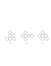
That is, if $H$ is nice-saturated then $H$ has exactly $\left\lfloor\frac{n-2}{k-1}\right\rfloor$ saturated cycles. As an example, a chemical $(6,4)$ -cactus with $p<\left\lfloor\frac{n-2}{k-1}\right\rfloor=1$ , a chemical $(6,4)$ -cactus in which the cut vertices on some polygon are not successively arranged, and a nice-saturated $(6,4)$ -cactus are illustrated as (a), (b) and (c), respectively, in Figure 1.

Refer to caption — Figure 1: (a). $p=0$ ; (b). The cut vertices on the $k$ -cycle $C$ are not successively arranged; (c). A nice-saturated $(6,4)$ -cactus.

Lemma 2.6.

A chemical cactus $H$ attains the maximum value of $n_{4,4}(H)$ if and only if $H$ is nice-saturated.

Proof.

Let $p$ and $d_{1},d_{2},\ldots,d_{s}$ be defined as above. By a simple calculation, we have

n_{4,4}(H)\leq kp+\sum_{v\in V(G),d(v)<k}(d(v)-1)=kp+(d_{1}-1)+(d_{2}-1)+\cdots+(d_{s}-1)

(7)

and the equality holds if and only if the cut vertices on each polygon of $H$ are successively arranged.

Suppose $p<\left\lfloor\frac{n-2}{k-1}\right\rfloor$ . Then by the pervious analysis, we have $d_{1}+d_{2}+\cdots+d_{s}-s\geq k-1$ . Let $d^{\prime}_{1},d^{\prime}_{2},\ldots,d^{\prime}_{s}$ be a sequence satisfying $d^{\prime}_{1}=k,1\leq d^{\prime}_{i}\leq d_{i}$ for $i\in\{2,3,\cdots,s\}$ and $\sum_{i=1}^{s}d^{\prime}_{i}=\sum_{i=1}^{s}d_{i}$ . Let S be the sequence obtained from the degree sequence of $T(H)$ by replacing $d_{1},d_{2},\ldots,d_{s}$ by $d^{\prime}_{1},d^{\prime}_{2},\ldots,d^{\prime}_{s}$ , respectively. It is clear that S is still a degree sequence of a tree with maximum degree not greater than $k$ . Let $H^{\prime}$ be a cactus such that $T(H^{\prime})$ has degree sequence S and the cut vertices on each polygon of $H^{\prime}$ are successively arranged. Then by (7) and a direct calculation, we have $n_{4,4}(H^{\prime})=n_{4,4}(H)+1$ . That is, $H$ does not attain the maximum value of $n_{4,4}(H)$ , which completes our proof. ∎

Theorem 2.1.

Let $G\in\mathcal{G}_{n,k}$ , where $n\geq 3$ and $k\geq 3$ . Then

SO_{\alpha}(G)\geq(4n-4)(2^{\alpha}+4^{\alpha})^{1/\alpha}+2(nk-4n+4)2^{1/\alpha}

~{}~{}~{}~{}~{}~{}~{}~{}~{}~{}+\left(6\times 2^{1/\alpha}-2(2^{\alpha}+4^{\alpha})^{1/\alpha}\right)\big{(}n-2+\left\lfloor\frac{n-2}{k-1}\right\rfloor\big{)},

and the equality holds if and only if $G$ is a nice-saturated chemical cactus.

Proof.

By (7), (5) and (6), if $G$ is minimum, then

n_{4,4}(G)=kp+(d_{1}-1)+(d_{2}-1)+\cdots+(d_{s}-1)=n-2+p=n-2+\left\lfloor\frac{n-2}{k-1}\right\rfloor.

Hence, the theorem follows directly from Corollary 2.1 and Lemma 2.6. ∎

3 Polygonal cactus with maximum general Sombor index

In this section we will characterize the polygonal cactus with maximum general Sombor index for the two cases $\alpha\geq 1,\beta>1$ ; and $\alpha=2,1/2\leq\beta<1$ , respectively.

Lemma 3.1.

Let $\Delta ABM$ be a triangle in Euclidean space and $O$ the midpoint of the triangle side $AB$ . Then $|MA|^{2\beta}+|MB|^{2\beta}>2|MO|^{2\beta}$ for any real number $\beta\geq\frac{1}{2}$ , where $|MA|$ is the length of the side $MA$ .

Proof.

Let $|MA|=a$ , $|MB|=b$ and $|MO|=d$ . When $a=b$ , the lemma follows directly. Without loss of generality, we now assume $a>b>0$ . By the triangle inequality, $d<\frac{a+b}{2}<a$ and so $(a,b)\rhd\left(\frac{a+b}{2},\frac{a+b}{2}\right)$ . Hence, by Lemma 2.1, $a^{2\beta}+b^{2\beta}\geq 2\left(\frac{a+b}{2}\right)^{2\beta}>2d^{2\beta}$ when $\beta\geq\frac{1}{2}.$ ∎

Lemma 3.2.

Let $s>2$ and $t>2$ . Then
(i). $r_{\alpha}(s+2,2;\beta)-r_{\alpha}(s-2,2;\beta)>0$ for any $\alpha>0$ and $\beta>0$ ;
(ii). $r_{\alpha}(s+2,t;\beta)+r_{\alpha}(s-2,t;\beta)\geq 2r_{\alpha}(s,t;\beta)$ for any $\alpha\geq 1$ and $\beta>1$ ;
(iii). $r_{\alpha}(s+2,t-2;\beta)+r_{\alpha}(s-2,t+2;\beta)\geq 2r_{\alpha}(s,t;\beta)$ for any $\alpha\geq 1$ and $\beta>1$ .

Proof.

(i) follows directly.

For (ii), by Lemma 2.1 and the monotonicity of $r_{\alpha}(s,t;\beta)$ , we have

$\displaystyle r_{\alpha}(s+2,t;\beta)+r_{\alpha}(s-2,t;\beta)$	$\displaystyle=$	$\displaystyle\left((s+2)^{\alpha}+t^{\alpha}\right)^{\beta}+\left((s-2)^{\alpha}+t^{\alpha}\right)^{\beta}$
		$\displaystyle\geq 2\left(\frac{(s+2)^{\alpha}+(s-2)^{\alpha}}{2}+t^{\alpha}\right)^{\beta}$
		$\displaystyle\geq 2(s^{\alpha}+t^{\alpha})^{\beta}$
		$\displaystyle=2r_{\alpha}(s,t;\beta).$

Hence, (ii) holds.

The discussion for (iii) is analogous to that for (ii). ∎

Theorem 3.1.

Let $n\geq 3,k\geq 3$ and $G\in\mathcal{G}_{n,k}$ . If $\alpha\geq 1$ and $\beta>1$ ; or $\alpha=2$ and $\frac{1}{2}\leq\beta<1$ , then

SO_{\alpha}(G;\beta)\leq 2n((2n)^{\alpha}+2^{\alpha})^{\beta}+n(k-2)(2^{\alpha+1})^{\beta}

and the equality holds if and only if $G\cong S_{n,k}$ .

Proof.

We first assume that $\alpha\geq 1$ and $\beta>1$ .

Let $G$ be such that $SO_{\alpha}(G;\beta)$ is as large as possible. Further, let $C_{1}=z_{1}z_{2}\cdots z_{k}z_{1}$ and $C_{2}=v_{1}v_{2}\cdots v_{k}v_{1}$ be two pendent polygons such that $d_{G}(C_{1},C_{2})$ is as large as possible, where $z_{1}$ and $v_{1}$ are the cut-vertices of $C_{1}$ and $C_{2}$ , respectively.

If $G\cong S_{n,k}$ , then the theorem follows directly. We now assume $G\not\cong S_{n,k}$ . Then, $z_{1}\neq v_{1}$ . Let $G_{1}=G-v_{1}v_{2}-v_{1}v_{k}+z_{1}v_{2}+z_{1}v_{k}$ and $G_{2}=G-z_{1}z_{2}-z_{1}z_{k}+v_{1}z_{2}+v_{1}z_{k}$ . We consider the following two cases:

Case 1. $z_{1}$ and $v_{1}$ are adjacent in $G$ .

In this case, we have $SO_{\alpha}(G_{1};\beta)-SO_{\alpha}(G;\beta)=$

	$\displaystyle\sum_{v\in N_{G}(v_{1})\setminus\{z_{1}\}}\left(r_{\alpha}\big{(}d_{G}(v_{1})-2,d_{G}(v);\beta\big{)}-r_{\alpha}\big{(}d_{G}(v_{1}),d_{G}(v);\beta\big{)}\right)$
	$\displaystyle+\sum_{z\in N_{G}(z_{1})\setminus\{v_{1}\}}\left(r_{\alpha}\big{(}d_{G}(z_{1})+2,d_{G}(z);\beta\big{)}-r_{\alpha}\big{(}d_{G}(z_{1}),d_{G}(z);\beta\big{)}\right)$
	$\displaystyle+2r_{\alpha}\big{(}d_{G}(z_{1})+2,2;\beta\big{)}-2r_{\alpha}\big{(}d_{G}(v_{1})-2,2;\beta\big{)}$
	$\displaystyle+r_{\alpha}\big{(}d_{G}(v_{1})-2,d_{G}(z_{1})+2;\beta\big{)}-r_{\alpha}\big{(}d_{G}(v_{1}),d_{G}(z_{1});\beta\big{)},\,\,\text{and}$

$SO_{\alpha}(G_{2};\beta)-SO_{\alpha}(G;\beta)=$

	$\displaystyle\sum_{v\in N_{G}(v_{1})\setminus\{z_{1}\}}\left(r_{\alpha}\big{(}d_{G}(v_{1})+2,d_{G}(v);\beta\big{)}-r_{\alpha}\big{(}d_{G}(v_{1}),d_{G}(v);\beta\big{)}\right)$
	$\displaystyle+\sum_{z\in N_{G}(z_{1})\setminus\{v_{1}\}}\left(r_{\alpha}\big{(}d_{G}(z_{1})-2,d_{G}(w);\beta\big{)}-r_{\alpha}\big{(}d_{G}(z_{1}),d_{G}(z);\beta\big{)}\right)$
	$\displaystyle+2r_{\alpha}\big{(}d_{G}(v_{1})+2,2;\beta\big{)}-2r_{\alpha}\big{(}d_{G}(z_{1})-2,2;\beta\big{)}$
	$\displaystyle+r_{\alpha}\big{(}d_{G}(v_{1})+2,d_{G}(z_{1})-2;\beta\big{)}-r_{\alpha}\big{(}d_{G}(v_{1}),d_{G}(z_{1});\beta\big{)}.$

Recall that $z_{1}$ and $v_{1}$ are the cut-vertices of $C_{1}$ and $C_{2}$ , respectively. Therefore, $d_{G}(z_{1})\geq 4$ and $d_{G}(v_{1})\geq 4$ . Combining with Lemma 3.2, we have

	$\displaystyle r_{\alpha}\big{(}d_{G}(v_{1})+2,d_{G}(v);\beta\big{)}+r_{\alpha}\big{(}d_{G}(v_{1})-2,d_{G}(v);\beta\big{)}>2r_{\alpha}\big{(}d_{G}(v_{1}),d_{G}(v);\beta\big{)},$
	$\displaystyle r_{\alpha}\big{(}d_{G}(z_{1})+2,d_{G}(z);\beta\big{)}+r_{\alpha}\big{(}d_{G}(z_{1})-2,d_{G}(z);\beta\big{)}>2r_{\alpha}\big{(}d_{G}(z_{1}),d_{G}(z);\beta\big{)},$
	$\displaystyle r_{\alpha}\big{(}d_{G}(v_{1})+2,d_{G}(z_{1})-2;\beta\big{)}+r_{\alpha}\big{(}d_{G}(v_{1})-2,d_{G}(z_{1})+2;\beta\big{)}>2r_{\alpha}\big{(}d_{G}(v_{1}),d_{G}(z_{1});\beta\big{)},$
	$\displaystyle r_{\alpha}\big{(}d_{G}(z_{1})+2,2;\beta\big{)}-r_{\alpha}\big{(}d_{G}(z_{1})-2,2;\beta\big{)}>0,\text{\quad and}$
	$\displaystyle r_{\alpha}\big{(}d_{G}(v_{1})+2,2;\beta\big{)}-r_{\alpha}\big{(}d_{G}(v_{1})-2,2;\beta\big{)}>0.$

This means that $SO_{\alpha}(G_{1};\beta)>SO_{\alpha}(G;\beta)$ or $SO_{\alpha}(G_{2};\beta)>SO_{\alpha}(G;\beta)$ , a contradiction.

Case 2. $z_{1}$ and $v_{1}$ are not adjacent in $G$ .

In this case, we have

$\displaystyle SO_{\alpha}(G_{1};\beta)-SO_{\alpha}(G;\beta)$	$\displaystyle=$	$\displaystyle\sum_{v\in N_{G}(v_{1})}\left(r_{\alpha}\big{(}d_{G}(v_{1})-2,d_{G}(v);\beta\big{)}-r_{\alpha}\big{(}d_{G}(v_{1}),d_{G}(v);\beta\big{)}\right)$
		$\displaystyle+\sum_{z\in N_{G}(z_{1})}\left(r_{\alpha}\big{(}d_{G}(z_{1})+2,d_{G}(z);\beta\big{)}-r_{\alpha}\big{(}d_{G}(z_{1}),d_{G}(z);\beta\big{)}\right)$
		$\displaystyle+2r_{\alpha}\big{(}d_{G}(z_{1})+2,2;\beta\big{)}-2r_{\alpha}\big{(}d_{G}(v_{1})-2,2;\beta\big{)},\,\,\text{and}$

$\displaystyle SO_{\alpha}(G_{2};\beta)-SO_{\alpha}(G;\beta)$	$\displaystyle=$	$\displaystyle\sum_{v\in N_{G}(v_{1})}\left(r_{\alpha}\big{(}d_{G}(v_{1})+2,d_{G}(v);\beta\big{)}-r_{\alpha}\big{(}d_{G}(v_{1}),d_{G}(v);\beta\big{)}\right)$
		$\displaystyle+\sum_{z\in N_{G}(z_{1})}\left(r_{\alpha}\big{(}d_{G}(z_{1})-2,d_{G}(z);\beta\big{)}-r_{\alpha}\big{(}d_{G}(z_{1}),d_{G}(z);\beta\big{)}\right)$
		$\displaystyle+2r_{\alpha}\big{(}d_{G}(v_{1})+2,2;\beta\big{)}-2r_{\alpha}\big{(}d_{G}(z_{1})-2,2;\beta\big{)}.$

Recall that $d_{G}(z_{1})\geq 4$ and $d_{G}(v_{1})\geq 4$ . Similar to Case 1, by Lemma 3.2 , we have

	$\displaystyle r_{\alpha}\big{(}d_{G}(v_{1})+2,d_{G}(v);\beta\big{)}+r_{\alpha}\big{(}d_{G}(v_{1})-2,d_{G}(v);\beta\big{)}>2r_{\alpha}\big{(}d_{G}(v_{1}),d_{G}(v);\beta\big{)},$
	$\displaystyle r_{\alpha}\big{(}d_{G}(z_{1})+2,d_{G}(z);\beta\big{)}+r_{\alpha}\big{(}d_{G}(z_{1})-2,d_{G}(z);\beta\big{)}>2r_{\alpha}\big{(}d_{G}(z_{1}),d_{G}(z);\beta\big{)},$
	$\displaystyle r_{\alpha}\big{(}d_{G}(z_{1})+2,2;\beta\big{)}-r_{\alpha}\big{(}d_{G}(z_{1})-2,2;\beta\big{)}>0\text{\quad and}$
	$\displaystyle r_{\alpha}\big{(}d_{G}(v_{1})+2,2;\beta\big{)}-r_{\alpha}\big{(}d_{G}(v_{1})-2,2;\beta\big{)}>0,$

which means that $SO_{\alpha}(G_{1};\beta)>SO_{\alpha}(G;\beta)$ or $SO_{\alpha}(G_{2};\beta)>SO_{\alpha}(G;\beta)$ , a contradiction.

Therefore, $S_{n,k}$ is the unique maximal polygonal cactus. Further, we have

SO_{\alpha}(S_{n,k};\beta)=2nr_{\alpha}(2n,2;\beta)+n(k-2)r_{\alpha}(2,2;\beta)=2n((2n)^{\alpha}+2^{\alpha})^{\beta}+n(k-2)(2^{\alpha+1})^{\beta}.

The discussion for the case that $\alpha=2$ and $\frac{1}{2}\leq\beta<1$ is analogous by Lemma 3.2 (i) and Lemma 3.1.∎

4 Polygonal cacti with minimum general Sombor index

A symmetric function $\varphi(s,t)$ defined on positive real numbers is called escalating [22] if

\displaystyle\varphi(s_{1},s_{2})+\varphi(t_{1},t_{2})\geq\varphi(s_{2},t_{1})+\varphi(s_{1},t_{2})

(8)

for any $s_{1}\geq t_{1}>0$ and $s_{2}\geq t_{2}>0,$ and the inequality holds if $s_{1}>t_{1}>0$ and $s_{2}>t_{2}>0$ . Further, an escalating function $\varphi(s,t)$ is called special escalating [23] if

\displaystyle 4\varphi(2l,2)-\varphi(2l-2,4)-\varphi(2l-2,2)-\varphi(4,2)-\varphi(4,4)\geq 0

(9)

for $l\geq 3$ and

\displaystyle\varphi(s_{1},s_{2})-\varphi(t_{1},t_{2})\geq 0

(10)

for any $s_{1}\geq t_{1}\geq 2$ and $s_{2}\geq t_{2}\geq 2$ .

Lemma 4.1.

If $s,t>0$ , then $r_{\alpha}(s,t;\beta)=\left(s^{\alpha}+t^{\alpha}\right)^{\beta}$ is special escalating for $\alpha\geq 1$ and $\beta>1$ .

Proof.

Set $\varphi(s,t)=\left(s^{\alpha}+t^{\alpha}\right)^{\beta}$ . Since $\alpha\geq 1$ and $\beta>1$ , we have $\big{(}s_{1}^{\alpha}+s_{2}^{\alpha},t_{1}^{\alpha}+t_{2}^{\alpha}\big{)}\rhd\big{(}s_{2}^{\alpha}+t_{1}^{\alpha},s_{1}^{\alpha}+t_{2}^{\alpha}\big{)}$ when $s_{1}>t_{1}>0$ and $s_{2}>t_{2}>0$ . Then by Lemma 2.1, the inequality in (8) strictly holds. Further, it is clear that the equality in (8) holds when $s_{1}=t_{1}>0$ or $s_{2}=t_{2}>0$ . This means that $\left(s^{\alpha}+t^{\alpha}\right)^{\beta}$ is escalating.

In addition, by Lemma 2.1 and the monotonicity of $\left(s^{\alpha}+t^{\alpha}\right)^{\beta}$ , if $l\geq 3$ and $\alpha\geq 1$ then $(2l)^{\alpha}+2^{\alpha}\geq(2l-2)^{\alpha}+4^{\alpha}>(2l-2)^{\alpha}+2^{\alpha}$ , $(2l)^{\alpha}+2^{\alpha}>4^{\alpha}+2^{\alpha}$ and $(2l)^{\alpha}+2^{\alpha}\geq 6^{\alpha}+2^{\alpha}\geq 4^{\alpha}+4^{\alpha}$ . Hence, (9) follows directly as $\beta>1$ .

Finally, it is easy to see that (10) holds when $\alpha\geq 1$ and $\beta>1$ by the monotonicity of $\left(s^{\alpha}+t^{\alpha}\right)^{\beta}$ . Therefore, $\left(s^{\alpha}+t^{\alpha}\right)^{\beta}$ is special escalating. ∎

A $k$ -polygonal cactus $G$ is called a cactus chain if each polygon in $G$ has at most two cut-vertices and each cut-vertex is the common vertex of exactly two polygons. It is clear that each cactus chain has exactly $n-2$ non-pendent polygons and two pendent polygons for $n\geq 2$ . We denote by $\mathcal{A}_{n,k}$ the class consisting of those cactus chains such that each pair of cut-vertices that lies in the same polygon of $G$ are adjacent. In contrast, we denote by $\mathcal{B}_{n,k}$ the class consisting of those cactus chains such that each pair of cut-vertices that lies in the same polygon of $G$ are not adjacent. It can be seen that $\mathcal{A}_{n,k}$ is unique for $k\geq 3$ and $\mathcal{B}_{n,3}=\emptyset$ .

Theorem 4.1.

[23] Let $f(s,t)$ be a special escalating function and $G$ be a cactus of $\mathcal{G}_{n,k}$ , where $n\geq 3$ and $k\geq 3$ .
(i). If $k=3$ , then

I_{f}(G)\geq 2f(2,2)+2nf(4,2)+(n-2)f(4,4)

with equality holding if and only if $G\in\mathcal{A}_{n,3}$ .
(ii). If $k\geq 4$ , then

I_{f}(G)\geq(kn-4n+4)f(2,2)+(4n-4)f(4,2),

where the equality holds if $G\in\mathcal{B}_{n,k}$ . Furthermore, if $k\in\{4,5\}$ , then the equality holds if and only if $G\in\mathcal{B}_{n,k}.$

Corollary 4.1.

Let $n\geq 3,k\geq 3,\alpha\geq 1,\beta>1$ and $G\in\mathcal{G}_{n,k}$ .
(i). If $k=3$ , then $SO_{\alpha}(G;\beta)\geq 2\big{(}2^{\alpha+1}\big{)}^{\beta}+2n\big{(}4^{\alpha}+2^{\alpha}\big{)}^{\beta}+(n-2)\big{(}2\cdot 4^{\alpha}\big{)}^{\beta}$ , where the equality holds if and only if $G\in\mathcal{A}_{n,3}$ .
(ii). If $k\geq 4$ , then $SO_{\alpha}(G;\beta)\geq(kn-4n+4)\big{(}2^{\alpha+1}\big{)}^{\beta}+(4n-4)\big{(}4^{\alpha}+2^{\alpha}\big{)}^{\beta}$ , where the equality holds if $G\in\mathcal{B}_{n,k}$ . Furthermore, if $k\in\{4,5\}$ , then the equality holds if and only if $G\in\mathcal{B}_{n,k}.$

Proof.

In Theorem 4.1, set $f(s,t)=r_{\alpha}(s,t;\beta)$ . Then the corollary follows immediately by Lemma 4.1 and a simple calculation. ∎

5 Acknowledgement

This work was supported by the National Natural Science Foundation of China [Grant number: 11971406].

References

[1] A. Ali, D. Dimitrov, On the extremal graphs with respect to bond incident degree indices, Discrete Appl. Math. 238 (2018) 32-40.
[2] R. Cruz, I. Gutman, J. Rada, Sombor index of chemical graphs, Appl. Math. Comput. 399 (2021) 126018.
[3] K.C. Das, A.S. Çevik, I.N. Cangul, Y. Shang, On Sombor index, Symmetry 13, 140 (2021), https://doi.org/10.3390/sym13010140.
[4] E. Deutsch, S. Klavžar, $M$ -polynomial revisited: Bethe cacti and an extension of Gutman’s approach, J. Appl. Math. Comput. 60 (2019) 253-264.
[5] S. Fajtlowicz, On conjectures of Graffiti-II, Congr. Numer. 60 (1987) 187-197.
[6] B. Furtula, I. Gutman, A forgotten topological index, J. Math. Chem. 53 (2015) 1184-1190.
[7] I. Gutman, Degree-based topological indices, Croat. Chem. Acta 86 (2013) 351-361.
[8] I. Gutman, J. Tošović, Testing the quality of molecular structure descriptors. Vertex-degree-based topological indices, J. Serb. Chem. Soc. 78 (2013) 805-810.
[9] I. Gutman, N. Trinajstić, Graph theory and molecular orbitals. Total $\pi$ -electron energy of alternant hydrocarbons, Chem. Phys. Lett. 17 (1972) 535-538.
[10] I. Gutman, Geometric approach to degree-based topological indices: Sombor indices, MATCH Commun. Math. Comput. Chem. 86 (2021) 11-16.
[11] J.C. Hernández, J.M. Rodríguez, O. Rosario, J.M. Sigarreta, Optimal inequalities and extremal problems on the general Sombor index, paper submitted arXiv:2108.05224.
[12] V.R. Kulli, The $(a,b)$ - $KA$ indices of polycyclic aromatic hydrocarbons and benzenoid systems, International Journal of Mathematics Trends and Technology 65 (2019) 115-120.
[13] V.R. Kulli, I. Gutman, Computation of Sombor indices of certain networks, SSRG Int. J. Appl. Chem. 8 (2021) 1-5.
[14] X. Li, J. Zheng, A unified approach to the extremal trees for different indices, MATCH Commun. Math. Comput. Chem. 54 (2005) 195-208.
[15] Z. Lin, T. Zhou, V.R. Kullic, L. Miao, On the first Banhatti-Sombor index, preprint arXiv:2104.03615.
[16] A.W. Marshall , I. Olkin, Inequalities: Theory of Majorization and Its Applications, Academic Press, New York, 1979.
[17] S. Nikolić, G. Kovačević, A. Miličević, N. Trinajstić, The Zagreb indices 30 years after, Croat. Chem. Acta 76 (2003) 113-124.
[18] M. Randić, On characterization of molecular branching, J. Amer. Chem. Soc. 97 (1975) 6609-6615.
[19] I. Redžpović, Chemical applicability of Sombor indices, J. Serb. Chem. Soc. 86 (2021) 445-457.
[20] T. Réti, T. Došlić, A. Ali, On the Sombor index of graphs, Contrib. Math. 3 (2021) 11-18.
[21] D. Vukičević, J. Durdević, Bond additive modeling 10. Upper and lower bounds of bond incident degree indices of catacondensed uoranthenes, Chem. Phys. Lett. 515 (2011) 186-189.
[22] H. Wang, Functions on adjacent vertex degrees of trees with given degree sequence, Cent. Eur. J. Math. 12 (2014) 1656-1663.
[23] J. Ye, M. Liu, Y. Yao, K.C. Das, Extremal polygonal cacti for bond incident degree indices, Discrete Appl. Math. 257 (2019) 289-298.
[24] B. Zhou, N. Trinajstić, On general sum-connectivity index, J. Math. Chem. 47 (2010) 210-218.

Extremal Polygonal Cacti for General Sombor Index***This paper was supported by the National Natural Science Foundation of China [No. 11971406].

Abstract

1 Introduction

2 Polygonal cacti with minimum α\alpha-Sombor index

Definition 2.1.

Lemma 2.1.

Lemma 2.2.

Proof.

Lemma 2.3.

Proof.

Lemma 2.4.

Proof.

Lemma 2.5.

Proof.

Corollary 2.1.

Lemma 2.6.

Proof.

Theorem 2.1.

Proof.

3 Polygonal cactus with maximum general Sombor index

Lemma 3.1.

Proof.

Lemma 3.2.

Proof.

Theorem 3.1.

Proof.

4 Polygonal cacti with minimum general Sombor index

Lemma 4.1.

Proof.

Theorem 4.1.

Corollary 4.1.

Proof.

5 Acknowledgement

References

Extremal Polygonal Cacti for General Sombor Index^*^**This paper was supported by the National Natural Science Foundation of China [No. 11971406].

2 Polygonal cacti with minimum $\alpha$ -Sombor index