Extracting the pole and Breit-Wigner properties of nucleon and resonances from the photoproduction
Abstract
We have developed a covariant isobar model to phenomenologically explain the four possible isospin channels of photoproduction. To obtain a consistent reaction amplitude, which is free from the lower-spin background problem, we used the consistent electromagnetic and hadronic interactions described in our previous report. We used all available experimental data, including the recent MAMI A2 2018 data obtained for the and isospin channels. By fitting the calculated observables to these data we extract the resonance properties, including their Breit-Wigner and pole parameters. Comparison of the extracted parameters with those listed by the Particle Data Group yields a nice agreement. An extensive comparison of the calculated observables with experimental data is also presented. By using the model we investigated the effects of three different form factors used in the hadronic vertex of each diagram. A brief discussion on the form factors is given.
pacs:
13.60.Le, 14.20.Gk, 25.20.LjI INTRODUCTION
For more than 50 years kaon photoproduction off a nucleon has gained a special interest in the hadronic physics community. Early theoretical work was reported in 1957 masasaki , but a more comprehensive analysis with fitting to experimental data was just started in 1966 thom . Since then many efforts have been devoted to explain this reaction, ranging from quark to hadronic coupled-channel models, as briefly mentioned in the introduction part of our previous report brief_intro .
In the beginning, the main motivations to study kaon photoproduction off the nucleon were merely to obtain theoretical explanation of the reaction process. However, it has been soon realized that an accurate theoretical model describing this elementary process is also useful in many branches of hadronic and nuclear physics. In hadronic physics the model is indispensable in the investigation of the missing resonances that have considerably large branching ratio to the strangeness channel missing-d13 , the narrow resonance which is also predicted to have a large branching ratio to the channel mart-narrow , and the resonance hadronic coupling constant that measures the strength of the interaction between kaon-hyperon final state and the resonance Mart:2013ida . In the nuclear physics this elementary model is required in calculating the cross section of hypernuclear photoproduction mart_hyp , which is the main observable in the investigation of hypernuclear spectroscopy.
Recently, the electroproduction on a tritium target, i.e, the process, has been performed at Jefferson Lab Hall A (JLab E12-17-003) and the result is currently being analyzed gogami . There have been intensive discussions on whether the system could be bound or would lead to a resonant state. Thus, this experiment is expected to shed light on the puzzle. Furthermore, an accurate measurement of hypertriton electroproduction has been proposed and conditionally approved as the JLab C12-19-002 experiment gogami . The experiment is expected to further elucidate the binding energy in the hypertriton, since the result of previous measurement indicated a stronger binding energy star . Therefore, an accurate elementary model, describing the photo- and electroproduction of kaon on the nucleon target is timely and urgently required.
Our previous model used to this end was Kaon-Maid maid , which includes kaon photo- and electroproduction off the nucleon in six isospin channels. However, due to tremendous increase in the number of experimental data, especially in the case of photoproduction, Kaon-Maid started to show its deficiency. To get rid of this problem we have started to improve the model in the photoproduction sector, for which experimental data dominate our present database.
In the previous works we have developed a new and modern covariant isobar model for kaon photoproduction off the nucleon and previous-work . The model fits nearly 9000 experimental data points and employs the consistent hadronic and electromagnetic interactions that eliminate contributions of high-spin resonance background Vrancx:2011qv ; Clymton:2017nvp . The latter is widely known as an intrinsic problem that plagues the formalism of high-spin propagators used to describe the contribution of nucleon and delta resonances. In this paper we extend the model, based on the covariant effective Lagrangian method, to include the other four isospin channels in the photoproduction.
We have organized this paper as follows. In Sec. II we discuss the formalism used in our model. In principle, we use the same interaction Lagrangians as described in our previous paper for the photoproduction, Clymton:2017nvp . In addition, we also briefly discuss the formalism used to extract resonance masses and widths at their pole positions in this section. In Sec. III we present the result of our analysis and compare the calculated observables with the available experimental data. To describe the accuracy of our model in details, an extensive comparison of polarization observables is given in this section. In Sec. IV we summarize our analysis and conclude the important findings. The extracted Breit-Wigner masses and widths of the resonances used in the model are listed in Table 7 of Appendix A.
II FORMALISM
II.1 The Model
In the present work we consider the photoproduction process of on a nucleon, i.e.,
| (1) |
Based on the isospin and strangeness conservations, Eq. (1) implies four different photoproduction processes given in Table 1.
| No. | Channel | (MeV) | (MeV) | |
|---|---|---|---|---|
| 1 | 1046 | 1686 | ||
| 2 | 1048 | 1687 | ||
| 3 | 1052 | 1691 | ||
| 4 | 1051 | 1690 |
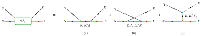
The scattering amplitude of these reactions is calculated from the first-order Feynman diagrams shown in Fig. 1. According to their intermediate states the diagrams can be grouped into three main channels, i.e., the -, - and -channel, with the corresponding Mandelstam variables are defined as
| (2) |
Note that the notation of the momenta written in Eq. (2) is given explicitly in Eq. (1). The corresponding vertex factors can be obtained from the effective Lagrangian approach, specifically by using the prescription given in Refs. Pascalutsa-PRD1998 ; Pascalutsa-PRC1999 ; Pascalutsa:2000kd . In our previous study of the photoproduction Clymton:2017nvp the Lagrangians were constructed according to the method proposed in Ref. Vrancx:2011qv in order to be consistent with the formulation of high spin () propagators. In the case of photoproduction, the hadronic and electromagnetic Lagrangians of the -channel spin- particle with positive parity reads
| (3) | |||||
| (4) | |||||
respectively, where is the field of the particle, is the antisymmetric tensor of photon field, and is the modified RS-field of spin- particles constructed to make the interaction consistent as proposed in Ref. Vrancx:2011qv . The modified RS-field reads
| (5) |
where is the original RS-field for spin- particles and the interaction operator is defined by
| (6) |
where and indicate the permutations of all possible and indices, respectively, and
| (7) |
The propagator used for calculating the scattering amplitude is obtained from the completeness relation of the RS-fields. This propagator, however, bears unphysical lower spin projection operator and eventually would yield unphysical contribution to the scattering amplitude if it was not properly handled. In this work, by using the interaction Lagrangians given by Eqs. (3) and (4), the remaining lower spin terms are automatically removed from the amplitude, leaving only the pure spin- contribution that comes from the projection operator
| (8) |
with the projection operator for spin- particle
| (9) |
where is equal to if is even and to if is odd, , and the coefficient is defined by
| (10) |
| Collaboration | Observable | Symbol | Channel | Reference | |
|---|---|---|---|---|---|
| LEPS 2003 | Photon asymmetry | 30 | Zegers:2003ux | ||
| CLAS 2004 | Differential cross section | 676 | McNabb:2003nf | ||
| Recoil polarization | 146 | McNabb:2003nf | |||
| SAPHIR 2004 | Differential cross section | 480 | Glander:2003jw | ||
| Recoil polarization | 12 | Glander:2003jw | |||
| CLAS 2006 | Differential cross section | 1280 | Bradford:2005pt | ||
| LEPS 2006 | Differential cross section | 39, 52 | Sumihama:2005er ; Kohri:2006yx | ||
| Photon asymmetry | 25, 26 | Sumihama:2005er ; Kohri:2006yx | |||
| Differential cross section | 72 | Kohri:2006yx | |||
| Photon asymmetry | 36 | Kohri:2006yx | |||
| SAPHIR 2006 | Differential cross section | 90 | Lawall:2005np | ||
| Recoil polarization | 10 | Lawall:2005np | |||
| CLAS 2007 | Beam-Recoil polarization | 94 | Bradford:2006ba | ||
| Beam-Recoil polarization | 94 | Bradford:2006ba | |||
| GRAAL 2007 | Recoil polarization | 8 | Lleres:2007tx | ||
| Photon asymmetry | 42 | Lleres:2007tx | |||
| CLAS 2010 | Differential cross section | 2089 | Dey:2010hh | ||
| Recoil polarization | 455 | Dey:2010hh | |||
| Differential cross section | 177 | AnefalosPereira:2009zw | |||
| Crystal Ball 2014 | Differential cross section | 1129 | Jude:2013jzs | ||
| CLAS 2016 | Recoil polarization | 127 | Paterson:2016vmc | ||
| Photon asymmetry | 127 | Paterson:2016vmc | |||
| Target asymmetry | 127 | Paterson:2016vmc | |||
| Beam-Recoil polarization | 127 | Paterson:2016vmc | |||
| Beam-Recoil polarization | 127 | Paterson:2016vmc | |||
| MAMI A2 2018 | Differential cross section | 39 | Akondi:2018shh | ||
| Differential cross section | 48 | Akondi:2018shh | |||
| Total number of data | 7784 | ||||
As mentioned above the constructed scattering amplitude is free from the unphysical lower-spin contribution that originates from the RS-fields. In the compact form the amplitude can be written as
| (11) | |||||
where is the four-momentum of resonance particle and the vertex factors and are derived directly from the interaction Lagrangians given by Eqs. (3) and (4), respectively. For the purpose of numerical computation of observables we need to calculate the total scattering amplitude, which is obtained by adding the background and resonance contributions, i.e.,
| (12) |
where the summation on the right hand side is performed over all nucleon resonances considered in the present work. The total amplitude is decomposed into the gauge and Lorentz invariant matrices
| (13) |
where denotes the gauge and Lorentz invariant matrices given by Clymton:2017nvp ; Mart:2019fau
| (14) | |||||
| (15) | |||||
| (16) | |||||
| (17) |
with and is the four dimensional Levi-Civita tensor. The required cross section and polarization observables can be calculated from the functions given by Eq. (13), which depend on the Mandelstam variables given in Eq. (2).
Note that as seen from Eq. (11) the present formalism introduces the high momentum dependence that might lead to a non-resonance behavior of scattering amplitude at high energies. To alleviate this problem we need a stronger hadronic form factor that can sufficiently suppresses the divergence of the amplitude at high energies. The widely use form factor is the dipole one, i.e.,
| (18) |
with the cutoff parameter and the resonance mass. However, we found that such a form factor does not have a sufficiently strong suppression for this purpose. Therefore, in this study we propose the use of the multi-dipole form factor
| (19) |
as well as the Gaussian one
| (20) |
and investigate the effects of these form factors on the constructed model. For the multi-dipole form factor we will present the result with , for which we obtained the best agreement with experimental data, and denote the model with HFF-P3. The models that use the form factors given by Eqs. (18) and (20) are denoted with HFF-P1 and HFF-G, respectively.
Equations (3) and (4) indicate that for each resonance with there are four unknown coupling constants which might be considered as free parameters. These coupling constants can be extracted from fitting the calculated observables to the corresponding experimental data. In the present work the fitting process was performed by using the CERN-MINUIT code James:1975dr to minimize the value of
| (21) |
where and indicate the numbers of experimental data and free parameters used in the fit, respectively, and are the -th values of experimental and theoretical observables, and is the corresponding experimental error bar.
Experimental data used in the present analysis are obtained from a number of experimental collaborations as listed in Table 2. Note that the photoproduction offers 4 possible isospin channels. Among them the channel has the largest number of experimental data, as can be seen in Table 2. Furthermore, experimental data of this channel are available for different types of observables, which can be expected to complete our understanding of this reaction. Nevertheless, although with a limited number and observable types, the existence of experimental data in the other three isospin channels is very important to constrain the extracted coupling constants as well as the predicted observables Mart:1995wu .
II.2 Resonances Properties
In this study, we extract a number of important resonance properties, i.e., their masses and total widths evaluated at pole, their partial widths, and their individual contribution to the process. The evaluation of mass and width at pole starts with a complex root equation of the denominator of the scattering amplitude, which reads
| (22) |
where and are the Breit-Wigner mass and width, respectively. The variable is defined as
| (23) |
where and are the mass and width evaluated at the pole, respectively. We can clearly see that the solutions of and were actually simple. However, in the present work, we use an energy-dependent width that is directly proportional to the total width Lee:2001 . As a consequence, we cannot analytically solve the root equation given in Eq. (22). Therefore, in the present analysis we solve this equation numerically.
Furthermore, we can also compute the partial decay widths to conveniently compare the values of extracted coupling constants in this study. To this end, we start with the interaction Lagrangians for spin resonances and for each we obtain the decay width formula. Note that in the present analysis we can only obtain the product of hadronic and electromagnetic decay widths, because in the single channel analysis only the product of the electromagnetic and hadronic coupling constants can be extracted. The formulation of these decay widths can be found in our previous study Clymton:2017nvp .
The significance of each resonance can be also evaluated by excluding the specific resonance in the fitting process. Mathematically, the significance of an resonance is defined through
| (24) |
where is obtained from fitting the data by using all resonances, while is obtained by using all but a specific resonance. In the present work Eq. (24) is also used for investigating the significance of resonances. The significance of a resonance is not only very useful for investigation of the role of each resonance in the reaction, but also for a practical guidance to simplify the model if minimizing the number of resonances used in the model is important. A simple covariant isobar model is very important for the application in few-body nuclear physics, for which numerical computation and accuracy are very demanding.
III RESULTS AND DISCUSSION
III.1 General Results
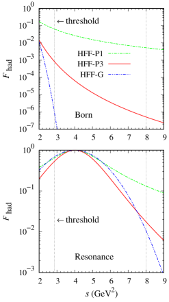
Table 3 compares the extracted coupling constants of the Born terms obtained for the 3 different hadronic form factor models. By comparing the values of , we can clearly see that the model HFF-P1 yields less agreement with experimental data. This indicates that to achieve a better agreement with experimental data we have to use a softer form factor. The result obtained from model HFF-P3 corroborates this. However, since the three form factors used in the present analysis have different forms, see Eqs. (18)-(20), it is difficult to estimate the suppression imposed by the form factors on the amplitude by merely comparing their cutoffs listed in Table 3. Therefore, in Fig. 2 we plot the form factors for both Born and resonance terms as a function of the Mandelstam variable and shows the energy region covered by the experimental data in the fitting database. From the top panel of Fig. 2 we may conclude that the Gaussian form factor is the softest one and, as a consequence, this form factor strongly suppresses the Born amplitude. In contrast to this form factor, the dipole one given by Eq. (18) provides the lightest suppression, whereas the multi-dipole form factor yields the relatively moderate suppression. Nevertheless, even the dipole form factor decreases the contribution of Born terms significantly. Thus, from Fig. 2 we may safely say that all models analyzed in this work are resonance-dominated models because, as shown in the bottom panel of Fig. 2, near the resonance mass the form factors do not suppress the amplitude significantly.
| Parameters | HFF-P1 | HFF-P3 | HFF-G |
|---|---|---|---|
| 0.90 | 1.30 | 1.30 | |
| 0.11 | 0.22 | ||
| 0.12 | |||
| 4.37 | 0.45 | ||
| (GeV) | 0.72 | 0.80 | 0.73 |
| (GeV) | 1.25 | 1.54 | 1.37 |
| (deg) | 90.0 | 90.0 | 53.4 |
| (deg) | 0.00 | 0.00 | 180.0 |
| 8657 | 8259 | 8282 | |
| 221 | 190 | 198 | |
| 158 | 146 | 153 | |
| 17 | 20 | 17 | |
| 1.22 | 1.16 | 1.16 |
In the case of resonance, within the covered energy the suppression effect of form factor is clearly not symmetrical. This is understandable because the resonance masses used in the present analysis are below 2.3 GeV. However, this asymmetrical suppression is required for the covariant description of a resonance due to the large contribution of a Z-diagram that indicates the existence of a particle and an antiparticle in the intermediate state Mart:2019jtb . This contribution increases quickly as the energy of resonance increases beyond the resonance mass and, therefore, requires an increasing suppression. In our previous study Mart:2019jtb it was shown that the dipole form factor given by Eq. (18) is suitable for this purpose.
In Table 3 we also show the contribution from each channel. It is apparent from this table that the model HFF-P3 shows the best agreement with the experimental data (lowest ) from all but the channel. As we will see later, when we compare the observables, the model deficiency in this channel originates from the discrepancy between the calculated differential cross section and the experimental data at forward angles. Nevertheless, the effect of this discrepancy is less significant compared to those obtained from the other three isospin channels. Furthermore, by analyzing the sources of experimental data we found that the model HFF-P3 yields a nice agreement not only with the SAPHIR Lawall:2005np , but also with the MAMI Akondi:2018shh data.
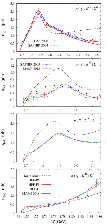
The calculated total cross sections obtained from the three models are compared with the available experimental data in Fig. 3. Note that although there are no data for the total cross section, both LEPS 2006 Kohri:2006yx and CLAS 2010 AnefalosPereira:2009zw collaborations have measured the differential cross section, whereas the LEPS 2006 collaboration has obtained the photon asymmetry Kohri:2006yx . Since these data have been included in our fitting database, we believe that the calculated total cross section shown in Fig. 3 is also accurate.
From Fig. 3 we may conclude that all three models can nicely reproduce the total cross section data. It is understandable that this new result is quite different from that of Kaon-Maid, since Kaon-Maid was fitted to the old SAPHIR data saphir98 ; Goers:1999sw , except for the reaction, for which Kaon-Maid yields a fairly good prediction to the recent MAMI data. We believe that the latter is pure coincidence and, in fact, the discrepancy between Kaon-Maid prediction and experimental data is clearly seen near the threshold and higher energy regions. It is also important to note that in the channel the total cross section indicates two resonance peaks. Interestingly, they originate from the and states that have been found to be important to describe both and photoproductions Mart:2019fau ; Mart:2000jv . The first peak does not appear in the channel, whereas the second one is shifted above 1.9 GeV due to the interference with other resonances, whose extracted masses are heavier than 1.9 GeV.
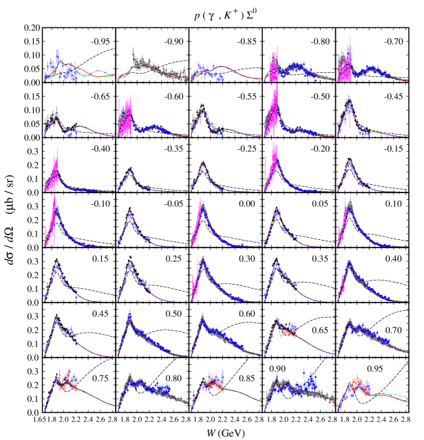
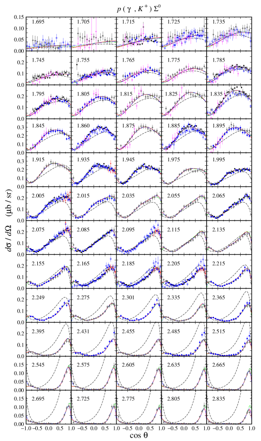
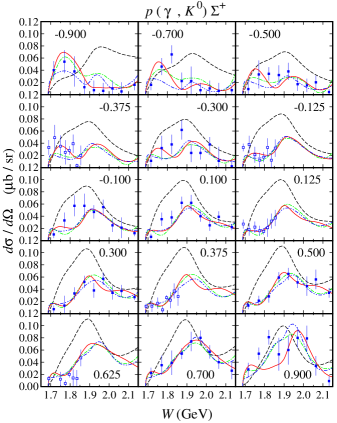
From Figs. 4 and 5 we can clearly see that all models do not exhibit significant variation in the differential cross sections, except for the extreme kinematics, i.e., in the forward and backward directions and in the higher energy region. In this kinematics, the interference between the resonance and background terms is found stronger than in any other regions. Meanwhile, experimental data in this kinematic are scattered and, in fact, in certain energy intervals there are no data available to constrain the models. Therefore, during the fitting process this condition yields significant variations among the models.
The lack of experimental data in certain energy and angular regions also occurs in the case of polarization observables. It is well known that unlike the cross section, the polarization observables are very sensitive to the ingredient of the reaction amplitude. Therefore, they can severely constrain the flexibility of the model during the fitting process. As a result, the calculated reported in the present work originates mostly from the polarization data.
From their formulations it is easy to understand that the single polarization observables are the simplest polarization observables that depend sensitively on all ingredients of the model, i.e., not only the resonance configuration, but also the background structure. Thus, they are very useful to constrain the models that predict similar trend in differential cross section, but significantly different beam, target, or recoil polarization observables. To this end, we also note that there was a discussion on whether the right model should be resonance- or background-dominated, or both resonance and background are equally contributing missing-d13 ; Mart:2017xtf ; Mart:ptep2019 . Hence, the observables can be used to help alleviate the problem. Furthermore, in the certain kinematical region, where differential cross section data are not available, single polarization observables provide an important tool to shape the trend of differential cross section.
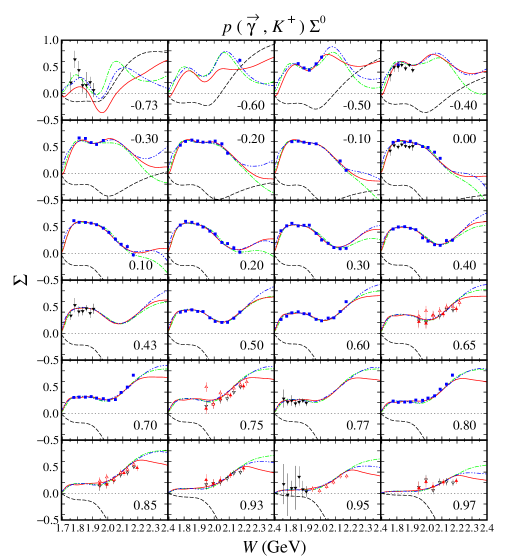
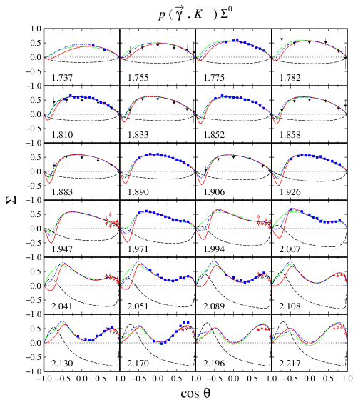
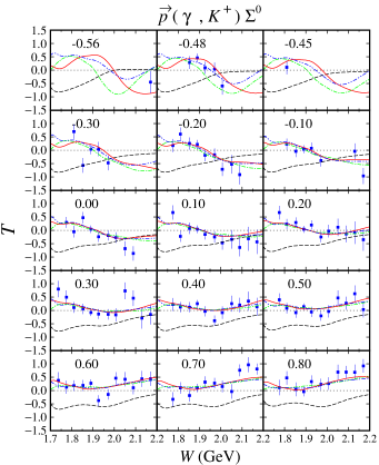
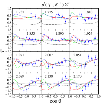
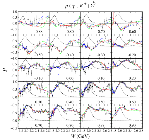
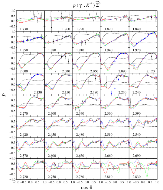
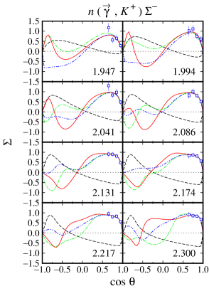
From Figs. 6 and 7 we found that in the kinematical region where the differential cross section data are abundant, e.g., at , the three models show a large variation of the calculated recoil polarization , in contrast to the predicted differential cross sections. On the other hand, in the kinematical region where differential cross section data are not available, e.g., at , we find that the models yield significant variation in both cross section and polarization observables. This phenomenon is also shown by the other single polarization observables, i.e., the photon asymmetry shown in Figs. 8 and 9, as well as the target asymmetry shown in Figs. 10 and 11. Therefore, we may conclude that single polarization observables are potential to become important tools to determine the correct ingredients of the Born and resonance terms in the photoproduction channels.
Double-polarization observables are even more sensitive to the constituent of the reaction amplitude compared to the single polarization ones. Therefore, double-polarization observables can be considered as the main constraint to the models.
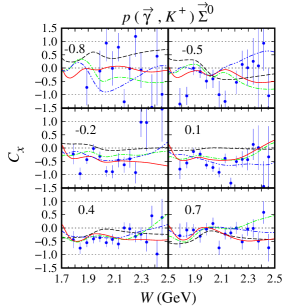
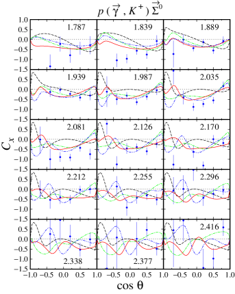
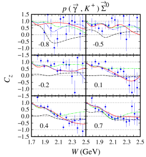
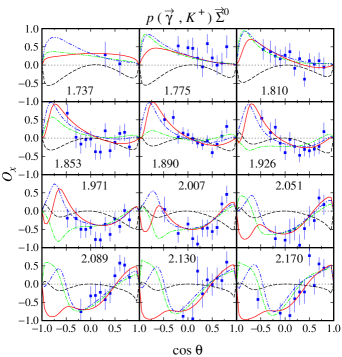
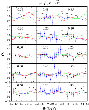
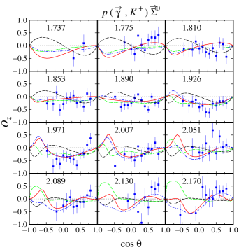
For the channels we notice that out of 12 possible double polarization observables, experimental data are only available for four types of the beam-recoil observables, i.e., , , , and . In the case of the and , unfortunately, the currently available experimental data have large error bars, especially in the extreme kinematics as shown in Figs. 12-15. As a consequence, all models investigated in the present work yield a large variance in this kinematics. As discussed before, the effect propagates to the calculated cross sections, for which large variation can be observed in the extreme kinematics (see Figs. 4 and 5). Furthermore, we also observe this effect in the recoil polarization as clearly shown in Figs. 6 and 7.
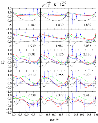
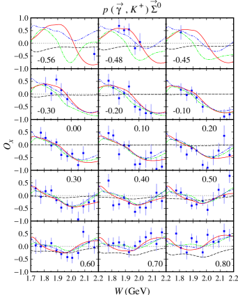
Unlike the double-polarization observables and , the available data for and are relatively more accurate, as shown in Figs. 16-19. We found that the three models have relatively similar trend in the region where experimental data are sufficiently available. However, a different situation is shown in the extreme kinematics, where experimental data are extremely scarce. Actually, the effects of this polarization is small only at the extreme kinematics, where the cross section data are accidentally scarce. Nevertheless, to obtain a more accurate model, including the background part, these data are urgently required, since contribution of the background part in this kinematic is stronger than in any other kinematical regions.
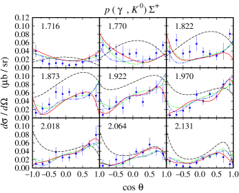
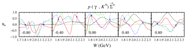
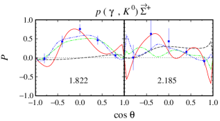
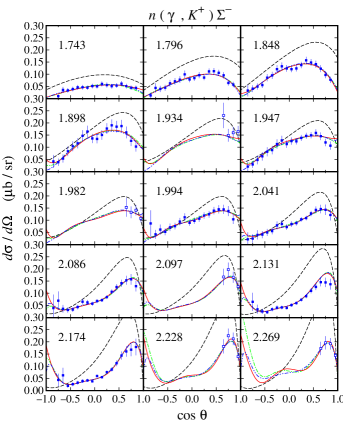
As stated before, the model HFF-P3 yields the best agreement with experimental data, although the difference is not large compared to the model HFF-G in the case of channel. From Figs. 20 and 21, we may conclude that contribution to the first peak in the differential cross section at GeV (see Fig. 20) stems mostly from the backward angles, since as shown in Fig. 21 the cross section in this energy region is backward peaking. The angular distributions of differential cross section obtained from the model HFF-P3 exhibit a clearer picture of the origin of both peaks in the total cross section. By comparing with the results from the other two models we might conclude that the difference between them originates from different ways of reproducing the recoil polarization data shown in Figs. 22-23, since, as shown in Figs. 20 and 21, both SAPHIR and MAMI data do not show significant discrepancy.
It is also obvious that at very forward and backward angles, only the model HFF-P3 shows different recoil polarization. The difference originates from the lack of data in the extreme kinematics from the MAMI collaboration. Thus, we might conclude that the different behavior shown by all models originates from the freedom to predict the missing data in the extreme kinematics.
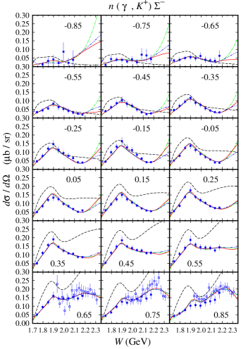
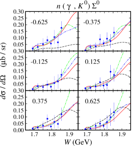
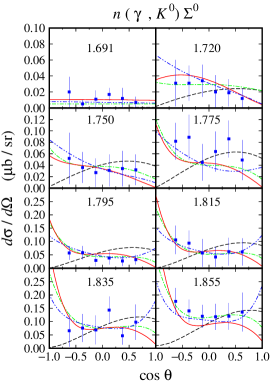
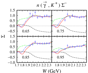
The other channels that use neutron as target exhibit a similar pattern as shown in Figs. 24-27. As expected, there are differences in the kinematical regions, where experimental data are lacking. Interestingly, we observe a unique behavior in the prediction of the model HFF-G for the , i.e., there are tiny peaks near the threshold region at backward and forward angles. The peaks, which will be discussed later when we discuss the resonances properties, originate from the contribution of high spin resonances which only appears near threshold in the model HFF-G. Unfortunately, this behavior cannot be further explored due to the lack of experimental data in this kinematics. As shown in Figs. 28 and 29, the same situation also happens in the case of the polarization asymmetry that usually provides a severe constraint to the model. Nevertheless, we will discuss this topic from another perspective in the following subsection.
III.2 Resonances Properties
Having constructed an isobar model that can nicely reproduce all photoproduction data we are in the position to study the properties of baryon resonances through their electromagnetic and hadronic interactions. The resonance properties that are of interest in the hadronic physics community are the resonance mass and width evaluated at its pole position as well as the extracted resonance partial decay width. Evaluation of the resonance mass and width at pole position has a clear advantage, since the result is model independent. Therefore, the properties of resonances evaluated at pole position in the present study are comparable with those obtained from other model-independent investigations.
The result is shown in Table 4, where we compare the resonance masses and widths evaluated at their poles obtained from the present work with those given by PDG. For completeness, we present the corresponding Breit-Wigner masses and widths in Table 7 of Appendix A. The calculated resonance masses show a good agreement with the PDG values, especially in the case of model HFF-G. On the other hand, the calculated widths show some discrepancies with the PDG ones. There is no obvious pattern observed in these discrepancies and, in fact, it seems to be random for all models. We believe that this phenomenon originates from the use of single channel analysis, where the resonance widths are not unitary defined. In the case of the current best models (HFF-G and HFF-P3), there are two adjacent resonances that show an interesting phenomenon, i.e., the and states. In these models the resonances produce different cross section behavior near the threshold by switching their pole positions. However, in the model HFF-G the pole positions of these resonances are closer to the PDG values. Put in other words, compared to other nucleon resonances the state is very likely to be important in the threshold region. Nevertheless, this finding still needs further investigation once the photoproduction data near threshold are sufficiently available.
| Resonances | PDG | HFF-P1 | HFF-P3 | HFF-G | |||||
|---|---|---|---|---|---|---|---|---|---|
| (MeV) | (MeV) | (MeV) | (MeV) | (MeV) | (MeV) | (MeV) | (MeV) | ||
| 1324 | 188 | 1351 | 206 | 1398 | 174 | ||||
| 1489 | 100 | 1489 | 100 | 1505 | 86 | ||||
| 1530 | 129 | 1530 | 129 | 1515 | 185 | ||||
| 1664 | 176 | 1658 | 121 | 1644 | 112 | ||||
| 1643 | 136 | 1651 | 114 | 1653 | 137 | ||||
| 1667 | 98 | 1655 | 108 | 1668 | 98 | ||||
| 1630 | 111 | 1635 | 97 | 1718 | 158 | ||||
| 1705 | 47 | 1679 | 41 | 1685 | 3 | ||||
| 1665 | 300 | 1712 | 222 | 1625 | 253 | ||||
| 1787 | 156 | 1773 | 162 | 1778 | 155 | ||||
| 1757 | 219 | 1757 | 219 | 1757 | 219 | ||||
| 1831 | 166 | 1887 | 204 | 1895 | 173 | ||||
| 1893 | 90 | 1893 | 124 | 1893 | 90 | ||||
| 1899 | 239 | 1918 | 148 | 1833 | 228 | ||||
| 2044 | 273 | 1978 | 167 | 1999 | 169 | ||||
| 1978 | 232 | 1963 | 229 | 1963 | 229 | ||||
| 1968 | 334 | 1937 | 322 | 1970 | 332 | ||||
| 2029 | 274 | 2031 | 274 | 2125 | 287 | ||||
| 2142 | 211 | 2142 | 211 | 2046 | 196 | ||||
| 2131 | 202 | 2130 | 197 | 2130 | 197 | ||||
| 2193 | 219 | 2265 | 229 | 2193 | 219 | ||||
| 1205 | 82 | 1211 | 81 | 1210 | 83 | ||||
| 1457 | 168 | 1454 | 171 | 1595 | 313 | ||||
| 1598 | 152 | 1626 | 152 | 1659 | 152 | ||||
| 1646 | 161 | 1602 | 211 | 1704 | 186 | ||||
| 1938 | 330 | 1938 | 330 | 1938 | 330 | ||||
| 1797 | 212 | 1801 | 177 | 1847 | 185 | ||||
| 1859 | 317 | 1875 | 269 | 1864 | 304 | ||||
| 1893 | 193 | 1873 | 290 | 1913 | 293 | ||||
| 1933 | 199 | 1971 | 205 | 1971 | 203 | ||||
| 1880 | 349 | 1840 | 332 | 1864 | 284 | ||||
| 1848 | 208 | 1907 | 179 | 1872 | 174 | ||||
| 2081 | 328 | 2196 | 237 | 2216 | 374 | ||||
| 2341 | 200 | 2378 | 204 | 2354 | 201 | ||||
| 2409 | 329 | 2409 | 329 | 2704 | 402 | ||||
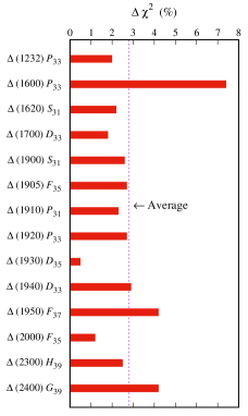
It is also interesting to explore how the resonances complement to each other through their significance in the photoproduction reaction. In Figs. 30-31 we show the significance of each resonance for the best model, i.e., model HFF-P3. We observe that in average the contribution of each resonance is relatively small, i.e., under . This is understandable since the number of resonances used in the model is large. As a consequence, the task to produce different structures in all calculated observables could be easily distributed to all resonances in the model. It is therefore obvious that the role of the excluded resonance will be immediately replaced by the adjacent one. Of course, there are a number of resonances that exhibit a relatively stronger or weaker significance compared to the other ones. For the stronger one, there is a resonance that contributes to the background because its mass is below the threshold energy, i.e., the state with . Apparently, the adjacent resonances cannot replace this resonance. As shown in Fig. 31, this resonance is the most important resonance in the present work.
From Table 4 we might expect that both and resonances could complement to each other. However, Figs. 30-31 indicate that they still have strong impact on the agreement between model calculation and experimental data. This can be understood because there are no resonances with spin equals to and adjacent mass. Another example that shows the importance of high spin resonances is exhibited by the state. This resonance has a relatively high significance compared to the other ones. By looking at the PDG estimate in Table 4 we obviously find that the extracted masses are significantly heavier. We note that this occurs in both Breit-Wigner and pole position methods. Furthermore, Table 4 also indicates that in the model HFF-G the extracted mass is about 500 MeV heavier than the PDG estimate. Therefore, we might conclude that this resonance is responsible for improving the agreement with experimental data in the higher energy region. Nevertheless, for a more conclusive finding, investigation at this energy region is strongly advocated in the future. Since we have observed similar cases in the present work, we might conclude that the high spin resonances are indispensable in the photoproduction process. The role of spin-7/2 and 9/2 resonances in the photoproduction has been thoroughly analyzed in Ref. Clymton:2017nvp . For spin-11/2 and 13/2 nucleon and delta resonances the analysis is still ongoing and will be published soon lala-2020 .
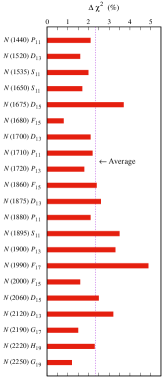
Figures 30 and 31 also show the less significance resonances, e.g., the and , which have less than . In the case of the resonance this is understandable, since it contributes to the background part of the model and, furthermore, there is a spin resonance with adjacent mass, i.e., the . For the resonance, although there is evidence for its branching to the channels, the present work indicates that this state is less significance. A closer look to the mass position reveals that the mass of this resonance lies among the masses of six resonances from 1900 to 1950 MeV (see Fig. 31). We believe that the less significance of the resonance originates from this phenomenon. As a consequence, if we needed to simplify the model but not its accuracy, this resonance could be excluded.
In Tables 5 and 6 we compare the resonance partial widths obtained in the present analysis and those listed by PDG. Table 5 shows the comparison for the proton channels, whereas Table 6 shows that for the neutron channels. Since the value of partial width for resonances is the same for both proton and neutron channels, we only show them in Table 5. From Tables 5 and 6, we may conclude that most of the extracted partial widths are in good agreement with those listed by PDG. Nevertheless, we also note that there are large discrepancies in the case of the , , and . This would be an interesting phenomenon for future investigation, since for the three resonances the discrepancies between our best model HFF-G and the PDG values are milder.
In our previous study Clymton:2017nvp we also observed a similar phenomenon, i.e., the extracted partial widths for a number of resonances are found to be very large. Presumably, this is caused by the large number of resonances involved in the model, which creates strong interferences among the resonances and causes irrelevant contribution of certain resonances at energy far from the resonance masses. In the present work we found that this problem can be overcome by using the Gaussian hadronic form factor given in the HFF-G model, which strongly suppresses the amplitude except near the resonance mass. Comparison among the three models given in Tables 5 and 6 shows that the Gaussian form factor reduces the extracted partial waves to the values closer to the PDG estimates, except for the resonance, for which the extracted value is still much larger than the PDG one. Therefore, future investigation should address this problem, since the is currently a four-star resonance.
| Resonances | () | ||||
|---|---|---|---|---|---|
| PDG | HFF-P1 | HFF-P3 | HFF-G | ||
| - | |||||
| - | |||||
| - | |||||
| - | |||||
| - | |||||
| - | |||||
| - | |||||
| - | |||||
| - | |||||
| - | |||||
| - | |||||
| - | |||||
| - | |||||
| - | |||||
| - | |||||
| - | |||||
| - | |||||
A closer look at Tables 5 and 6 reveals that the resonance experiences the strongest reduction if we use the Gaussian form factor (model HFF-G). Compared to the model HFF-P3 the fractional decay width of this resonance is reduced by more than . This is due to the change of the resonance role, between the and states as we mentioned earlier. Since the is closer to the threshold, the branching ratio to this reaction tends to be smaller. In addition to this fact and earlier analysis, we have more confidence to say that the state is more likely to be found near the reaction threshold.
| Resonances | () | ||||
|---|---|---|---|---|---|
| PDG | HFF-P1 | HFF-P3 | HFF-G | ||
| - | |||||
| - | |||||
| - | |||||
| - | |||||
| - | |||||
| - | |||||
| - | |||||
| - | |||||
| - | |||||
IV SUMMARY AND CONCLUSION
We have analyzed the photoproduction data for all four possible isospin channels by using a covariant isobar model and including all appropriate nucleon and delta resonances. We used the consistent Lagrangians for hadronic and electromagnetic interactions to eliminate the problem of lower-spin background contribution. In this analysis, three different form factors have been used in the hadronic vertices, i.e., the dipole, multi-dipole, and Gaussian ones. The present model yields a nice agreement between calculated observables and experimental data. The best agreement is shown by the models that employ the multidipole and Gaussian form factors. We have also extracted the Breit-Wigner masses and widths of the nucleon and delta resonances as well as their masses and widths at their pole positions. By comparing the extracted values with those given by PDG we conclude that the Gaussian form factor leads to a better agreement. This indicates that the resonances included in the model require a strong suppression from the form factors, which is a typical behavior of the phenomenological model that employs a large number of resonances.
V ACKNOWLEDGMENTS
The work of S.C. was supported in part by the Indonesian Endowment Fund for Education (LPDP). T.M. is supported by the PUTI Q2 Grant of Universitas Indonesia, under contract No. NKB-1652/UN2.RST/HKP.05.00/2020.
Appendix A The Extracted Masses and Widths
The extracted Breit-Wigner masses and widths of the included nucleon and delta resonances in the model are listed in Table 7.
| Resonances | HFF-P1 | HFF-P3 | HFF-G | ||||
|---|---|---|---|---|---|---|---|
| Mass (MeV) | Width (MeV) | Mass (MeV) | Width (MeV) | Mass (MeV) | Width (MeV) | ||
| 1420 | 450 | 1450 | 450 | 1450 | 250 | ||
| 1510 | 125 | 1510 | 125 | 1520 | 100 | ||
| 1545 | 125 | 1545 | 125 | 1545 | 175 | ||
| 1670 | 170 | 1661 | 119 | 1648 | 110 | ||
| 1670 | 165 | 1670 | 130 | 1680 | 165 | ||
| 1686 | 120 | 1680 | 140 | 1687 | 120 | ||
| 1650 | 129 | 1650 | 109 | 1750 | 191 | ||
| 1710 | 50 | 1691 | 104 | 1687 | 50 | ||
| 1750 | 400 | 1750 | 248 | 1700 | 361 | ||
| 1829 | 220 | 1820 | 239 | 1820 | 220 | ||
| 1820 | 320 | 1820 | 320 | 1820 | 320 | ||
| 1856 | 180 | 1915 | 216 | 1914 | 180 | ||
| 1893 | 90 | 1893 | 123 | 1893 | 90 | ||
| 1930 | 250 | 1929 | 150 | 1870 | 250 | ||
| 2125 | 400 | 2010 | 200 | 2031 | 200 | ||
| 2044 | 335 | 2030 | 335 | 2030 | 335 | ||
| 2060 | 450 | 2030 | 450 | 2060 | 444 | ||
| 2075 | 305 | 2077 | 305 | 2165 | 305 | ||
| 2200 | 300 | 2200 | 300 | 2105 | 300 | ||
| 2204 | 369 | 2200 | 350 | 2200 | 350 | ||
| 2250 | 300 | 2320 | 300 | 2250 | 300 | ||
| 1230 | 120 | 1234 | 114 | 1234 | 120 | ||
| 1500 | 220 | 1500 | 229 | 1686 | 420 | ||
| 1600 | 150 | 1628 | 150 | 1660 | 150 | ||
| 1686 | 213 | 1686 | 400 | 1750 | 246 | ||
| 1920 | 325 | 1920 | 325 | 1920 | 325 | ||
| 1878 | 400 | 1855 | 270 | 1900 | 270 | ||
| 1910 | 340 | 1910 | 281 | 1910 | 322 | ||
| 1908 | 195 | 1910 | 300 | 1945 | 297 | ||
| 1963 | 220 | 2000 | 223 | 2000 | 220 | ||
| 1994 | 520 | 1954 | 520 | 1940 | 380 | ||
| 1915 | 335 | 1950 | 235 | 1915 | 235 | ||
| 2192 | 525 | 2240 | 275 | 2325 | 525 | ||
| 2393 | 275 | 2429 | 275 | 2405 | 275 | ||
| 2502 | 463 | 2502 | 463 | 2784 | 463 | ||
References
- (1) M. Kawaguchi and M. J. Moravcsik, Phys. Rev. 107, 563 (1957).
- (2) H. Thom, Phys. Rev. 151, 1322 (1966).
- (3) T. Mart, Phys. Rev. C 82, 025209 (2010); Phys. Rev. C 90, 065202 (2014).
- (4) T. Mart and C. Bennhold, Phys. Rev. C 61, 012201 (1999).
- (5) T. Mart, Phys. Rev. D 83, 094015 (2011); 88, 057501 (2013).
- (6) T. Mart, Phys. Rev. C 87, 042201(R) (2013).
- (7) T. Mart and B. I. S. van der Ventel, Phys. Rev. C 78 014004, (2008); T. Mart, L. Tiator, D. Drechsel and C. Bennhold, Nucl. Phys. A 640, 235 (1998).
- (8) T. Gogami et al. [HKS Collaboration], AIP Conf. Proc. 2319, 080019 (2021).
- (9) J. Adam et al., Nat. Phys. 16, 409 (2020).
- (10) T. Mart, C. Bennhold, H. Haberzettl, and L. Tiator, Kaon-Maid. Available at http://www.kph.uni-mainz.de/MAID/kaon/kaonmaid.html.
- (11) T. Mart, Phys. Rev. D 100, 056008 (2019).
- (12) T. Vrancx, L. De Cruz, J. Ryckebusch and P. Vancraeyveld, Phys. Rev. C 84, 045201 (2011).
- (13) S. Clymton and T. Mart, Phys. Rev. D 96, 054004 (2017).
- (14) V. Pascalutsa, Phys. Rev. D 58, 096002 (1998).
- (15) V. Pascalutsa and R. Timmermans, Phys. Rev. C 60, 042201 (1999).
- (16) V. Pascalutsa, Phys. Lett. B 503, 85 (2001).
- (17) R. G. T. Zegers et al. [LEPS Collaboration], Phys. Rev. Lett. 91, 092001 (2003).
- (18) J. W. C. McNabb et al. [CLAS Collaboration], Phys. Rev. C 69, 042201 (2004).
- (19) K. H. Glander et al., Eur. Phys. J. A 19, 251 (2004).
- (20) R. Bradford et al. [CLAS Collaboration], Phys. Rev. C 73, 035202 (2006).
- (21) M. Sumihama et al. [LEPS Collaboration], Phys. Rev. C 73, 035214 (2006).
- (22) H. Kohri et al., Phys. Rev. Lett. 97, 082003 (2006).
- (23) R. Lawall et al., Eur. Phys. J. A 24, 275 (2005).
- (24) R. K. Bradford et al. [CLAS Collaboration], Phys. Rev. C 75, 035205 (2007).
- (25) A. Lleres et al., Eur. Phys. J. A 31, 79 (2007).
- (26) B. Dey et al. [CLAS Collaboration], Phys. Rev. C 82, 025202 (2010).
- (27) S. A. Pereira et al. [CLAS Collaboration], Phys. Lett. B 688, 289 (2010).
- (28) T. C. Jude et al. [Crystal Ball at MAMI Collaboration], Phys. Lett. B 735, 112 (2014).
- (29) C. A. Paterson et al. [CLAS Collaboration], Phys. Rev. C 93, 065201 (2016).
- (30) C. S. Akondi et al. [A2 Collaboration], Eur. Phys. J. A 55, 202 (2019).
- (31) T. Mart and M. J. Kholili, J. Phys. G 46, 105112 (2019).
- (32) F. James and M. Roos, Comput. Phys. Commun. 10, 343 (1975).
- (33) T. Mart, C. Bennhold, and C. E. Hyde-Wright, Phys. Rev. C 51, R1074 (1995).
- (34) F. X. Lee, T. Mart, C. Bennhold, H. Haberzettl and L. E. Wright, Nucl. Phys. A 695, 237 (2001).
- (35) T. Mart, J. Kristiano and S. Clymton, Phys. Rev. C 100, 035207 (2019); J. Kristiano, S. Clymton, and T. Mart, Phys. Rev. C 96, 052201(R) (2017).
- (36) M. Q. Tran et al. [SAPHIR Collaboration], Phys. Lett. B 445, 20 (1998).
- (37) S. Goers et al. [SAPHIR Collaboration], Phys. Lett. B 464, 331 (1999).
- (38) T. Mart, Phys. Rev. C 62, 038201 (2000).
- (39) T. Mart and A. Rusli, Prog. Theor. Exp. Phys. 2017, 123D04 (2017).
- (40) T. Mart, Prog. Theor. Exp. Phys. 2019, 069101 (2019).
- (41) M. Tanabashi et al. [Particle Data Group], Phys. Rev. D 98 030001 (2018).
- (42) N. H. Luthfiyah and T. Mart, AIP Conf. Proc. 2234, 040015 (2020).